
0 Algorithms in Bioinformatics, Uni Tu¨bingen, Daniel Huson,...
141
0 Algorithms in Bioinformatics, Uni T¨ ubingen, Daniel Huson, SS 2004 Algorithms in Bioinformatics II Summer Semester 2004, ZBIT- Center for Bioinformatics T¨ ubingen, WSI-Informatik, Universit¨ at T¨ ubingen Prof. Dr. Daniel Huson [email protected]
Transcript of 0 Algorithms in Bioinformatics, Uni Tu¨bingen, Daniel Huson,...

0 Algorithms in Bioinformatics, Uni Tubingen, Daniel Huson, SS 2004
Algorithms inBioinformatics II
Summer Semester 2004,ZBIT- Center for Bioinformatics Tubingen,
WSI-Informatik, Universitat Tubingen
Prof. Dr. Daniel Huson

Algorithms in Bioinformatics, Uni Tubingen, Daniel Huson, SS 2004 1
13 Markov chains and Hidden Markov Models
We will discuss:
• Markov chains
• Hidden Markov Models (HMMs)
• Profile HMMs
This chapter is based on: S. Durbin, S. Eddy, A. Krogh and G. Mitchison, Biological SequenceAnalysis, Cambridge, 1998
13.1 Markov chains
Example: finding CpG-islands in the human genome.
Double stranded DNA:
...ApCpCpApTpGpApTpGpCpApGpGpApCpTpTpCpCpApTpCpGpTpTpCpGpCpGp...
...| | | | | | | | | | | | | | | | | | | | | | | | | | | | | ...
...TpGpGpTpApCpTpApCpGpTpCpCpTpGpApApGpGpTpApGpCpApApGpCpGpCp...
The C in a CpG pair is often modified by methylation (that is, an H-atom is replaced by a CH3-group). There is a relatively high chance that the methyl-C will mutate to a T . Hence, CpG pairs areunder-represented in the human genome.
Upstream of a gene, the methylation process is suppressed in short regions of the genome of length100-5000. These areas are called CpG-islands and they are characterized by the fact that we see moreCpG-pairs in them then elsewhere.
13.2 CpG-islands
CpG-islands are useful marks for genes in organisms whose genomes contain 5-methyl-cytosine.
CpG-islands in the promoter-regions of genes play an important role in the deactivation of a copy ofthe X-chromosome in females, in imprinting and in the deactivation of intra-genomic parasites.
Classical definition: DNA sequence of length 200 with a C+ G content of 50% and a ratio of observed-to-expected number of CpG’s that is above 0.6. (Gardiner-Garden & Frommer, 1987)
According to a recent study, human chromosomes 21 and 22 contain about 1100 CpG-islands and about750 genes. (Comprehensive analysis of CpG islands in human chromosomes 21 and 22, D. Takai & P. A. Jones,
PNAS, March 19, 2002)

2 Algorithms in Bioinformatics, Uni Tubingen, Daniel Huson, SS 2004
13.3 Questions
1. Given a short segment of genomic sequence. How to decide whether this segment comes from aCpG-island or not?
2. Given a long segment of genomic sequence. How to find all contained CpG-islands?
13.4 Markov chains
Our goal is to set up a probabilistic model for CpG-islands. Because pairs of consecutive nucleotidesare important in this context, we need a model in which the probability of one symbol depends on theprobability of its predecessor. This leads us to a Markov chain.
Example:
A C
G T
Circles= states, e.g. with names A , C , G and T .Arrows= possible transitions, each labeled with a transition probability ast = P (xi = t | xi−1 = s).
Definition A (time-homogeneous) Markov chain (of order 1) is a system (S, A) consisting of a finiteset of states S = s1, s2, . . . , sn and a transition matrix A = ast with
∑
t∈S ast = 1 for all s ∈ S,that determines the probability of the transition s→ t as follows:
P (xi+1 = t | xi = s) = ast.
(At any time i the chain is in a specific state xi and at the tick of a clock the chain changes to state xi+1
according to the given transition probabilities).
Example Weather in Tubingen, daily at midday: Possible states are rain, sun, clouds or tornado.
Transition probabilities:
R S C TR .5 .1 .4 0S .2 .6 .2 0C .3 .3 .4 0
Weather: ...rrrrrrccsssssscscscccrrcrcssss...
Given a sequence of states x1, x2, x3, . . . , xL. What is the probability that a Markov chain will stepthrough precisely this sequence of states?

Algorithms in Bioinformatics, Uni Tubingen, Daniel Huson, SS 2004 3
P (x) = P (xL, xL−1, . . . , x1)
= P (xL | xL−1, . . . , x1)P (xL−1 | xL−2, . . . , x1) . . . P (x1),
(by repeated application of P (X,Y ) = P (X|Y )P (Y ))
= P (xL, | xL−1)P (xL−1 | xL−2) . . . P (x2 | x1)P (x1)
= P (x1)∏L
i=2 axi−1xi,
because P (xi | xi−1, . . . , x1) = P (xi | xi−1) = axi−1xi, the Markov chain property!
13.5 Modeling the begin and end states
In the previous discussion we overlooked the fact that a Markov chain starts in some state x1, withinitial probability of P (x1).
We add a begin state to the model that is labeled ’b’. We will always assume that x0 = b holds. Then:
P (x1 = s) = abs = P (s),
where P (s) denotes the background probability of symbol s.
Similarly, we explicitly model the end of the sequence of states using an end state ’e’. Thus, theprobability that we end in state t is
P (xL = t) = axLe.
13.6 Extension of the model
Example:
A C
G T
eb
# Markov chain that generates CpG islands
# (Source: DEKM98, p 50)
# Number of states:
6
# State labels:
A C G T * +

4 Algorithms in Bioinformatics, Uni Tubingen, Daniel Huson, SS 2004
# Transition matrix:
0.1795 0.2735 0.4255 0.1195 0 0.002
0.1705 0.3665 0.2735 0.1875 0 0.002
0.1605 0.3385 0.3745 0.1245 0 0.002
0.0785 0.3545 0.3835 0.1815 0 0.002
0.2495 0.2495 0.2495 0.2495 0 0.002
0.0000 0.0000 0.0000 0.0000 0 1.000
13.7 Determining the transition matrix
The transition matrix A+ for DNA that comes from a CpG-island, is determined as follows:
a+st =
c+st∑
t′ c+st′
,
where cst is the number of positions in a training set of CpG-islands at which state s is followed bystate t.
We obtain A− empirically in a similar way.
13.8 Two examples of Markov chains
# Markov chain for CpG islands # Markov chain for non-CpG islands
# (Source: DEKM98, p 50) # (Source: DEKM98, p 50)
# Number of states: # Number of states:
6 6
# State labels: # State labels:
A C G T * + A C G T * +
# Transition matrix: # Transition matrix:
.1795 .2735 .4255 .1195 0 0.002 .2995 .2045 .2845 .2095 0 .002
.1705 .3665 .2735 .1875 0 0.002 .3215 .2975 .0775 .0775 0 .002
.1605 .3385 .3745 .1245 0 0.002 .2475 .2455 .2975 .2075 0 .002
.0785 .3545 .3835 .1815 0 0.002 .1765 .2385 .2915 .2915 0 .002
.2495 .2495 .2495 .2495 0 0.002 .2495 .2495 .2495 .2495 0 .002
.0000 .0000 .0000 .0000 0 1.000 .0000 .0000 .0000 .0000 0 1.00
13.9 Answering question 1
Given a short sequence x = (x1, x2, . . . , xL). Does it come from a CpG-island (model+)?
P (x | model+) =L∏
i=0
axixi+1,
with x0 = b and xL+1 = e.
We use the following score:
S(x) = logP (x | model+)
P (x | model−)=
L∑
i=0
loga+
xi−1xi
a−xi−1xi
.

Algorithms in Bioinformatics, Uni Tubingen, Daniel Huson, SS 2004 5
The higher this score is, the higher the probability is, that x comes from a CpG-island.
13.10 Questions that a Markov chain can answer
Example weather in Tubingen, daily at midday: Possible states are rain, sun or clouds.
Transition probabilities:
R S C
R .5 .1 .4S .2 .6 .2C .3 .3 .4
Types of questions that the model can answer:
If it is sunny today, what is the probability that the sun will shine for the next seven days?
How large is the probability, that it will rain for a month?
13.11 Hidden Markov Models (HMM)
Motivation: Question 2, how to detect CpG-islands inside a long sequence?
E.g., window techniques: a window of width w is moved along the sequence and the score is plotted.Problem: it is hard to determine the boundaries of CpG-islands, which window size w should onechoose?. . .
Approach: Merge the two Markov chains model+ and model− to obtain a so-called Hidden MarkovModel.
13.12 Hidden Markov Models
Definition A HMM is a system M = (S, Q,A, e) consisting of
• an alphabet S,
• a set of states Q,
• a matrix A = akl of transition probabilities akl for k, l ∈ Q, and
• an emission probability ek(b) for every k ∈ Q and b ∈ S.
13.13 Example
An HMM for CpG-islands:

6 Algorithms in Bioinformatics, Uni Tubingen, Daniel Huson, SS 2004
A C TG
A C TG+ + + +
− − − −
(Additionally, we have all transitions between states in either of the two sets that carry over from thetwo Markov chains model+ and model−.)
13.14 HMM for CpG-islands
# Number of states:
9
# Names of states (begin/end, A+, C+, G+, T+, A-, C-, G- and T-):
0 A C G T a c g t
# Number of symbols:
4
# Names of symbols:
a c g t
# Transition matrix, probability to change from +island to -island (and vice versa) is 10E-4
0.0000000000 0.0725193101 0.1637630296 0.1788242720 0.0754545682 0.1322050994 0.1267006624 0.1226380452 0.1278950131
0.0010000000 0.1762237762 0.2682517483 0.4170629371 0.1174825175 0.0035964036 0.0054745255 0.0085104895 0.0023976024
0.0010000000 0.1672435130 0.3599201597 0.2679840319 0.1838722555 0.0034131737 0.0073453094 0.0054690619 0.0037524950
0.0010000000 0.1576223776 0.3318881119 0.3671328671 0.1223776224 0.0032167832 0.0067732268 0.0074915085 0.0024975025
0.0010000000 0.0773426573 0.3475514486 0.3759440559 0.1781818182 0.0015784216 0.0070929071 0.0076723277 0.0036363636
0.0010000000 0.0002997003 0.0002047952 0.0002837163 0.0002097902 0.2994005994 0.2045904096 0.2844305694 0.2095804196
0.0010000000 0.0003216783 0.0002977023 0.0000769231 0.0003016983 0.3213566434 0.2974045954 0.0778441558 0.3013966034
0.0010000000 0.0002477522 0.0002457542 0.0002977023 0.0002077922 0.2475044955 0.2455084915 0.2974035964 0.2075844156
0.0010000000 0.0001768232 0.0002387612 0.0002917083 0.0002917083 0.1766463536 0.2385224775 0.2914165834 0.2914155844
# Emission probabilities:
0 0 0 0
1 0 0 0
0 1 0 0
0 0 1 0
0 0 0 1
1 0 0 0
0 1 0 0
0 0 1 0
0 0 0 1
From now one we use 0 for the begin and end state.
13.15 Example fair/loaded dice
Casino uses two dice, fair and loaded:
1: 1/62: 1/63: 1/64: 1/65: 1/66: 1/6
1: 1/102: 1/103: 1/104: 1/105: 1/106: 1/2
0.05
0.1
0.95 0.9
UnfairFair
Casino guest only observes the number rolled:

Algorithms in Bioinformatics, Uni Tubingen, Daniel Huson, SS 2004 7
6 4 3 2 3 4 6 5 1 2 3 4 5 6 6 6 3 2 1 2 6 3 4 2 1 6 6...
Which dice was used remains hidden:
F F F F F F F F F F F F U U U U U F F F F F F F F F F...
13.16 Example urns model
Given p urns U1, U2, . . . , Up. Each urn Ui contains ri red, gi green and bi blue balls. An urn Ui israndomly selected and from it a random ball k is taken (with replacement). The color of the ball k isreported.
r2 redg2 greenb2 blue
rp redgp greenbp blue
r1 redg1 greenb1 blue
...
r r g g b b g b g g g b b b r g r g b b b g g b g g b...
Again, (a part of) the actual state (namely which urn was chosen) is hidden.
13.17 HMM for the urns model
# Four urns
# Number of states:
5
# Names of states:
# (0 begin/end, and urns A-D)
0 A B C D
# Number of symbols:
3
# red, green, blue
r g b
# Transition matrix:
0 .25 .25 .25 .25
0.01 .69 .30 0 0
0.01 0 .69 .30 0
0.01 0 0 .69 .30
0.01 .30 0 0 .69
# Emission probabilities:
0 0 0
.8 .1 .1
.2 .5 .3
.1 .1 .8
.3 .3 .4
# EOF

8 Algorithms in Bioinformatics, Uni Tubingen, Daniel Huson, SS 2004
13.18 Generation of simulated data
We can use HMMs to generate data:
Algorithm
Start in state 0.
While we have not reentered state 0:
Choose a new state using the transition probabilities
Choose a symbol using the emission probabilities and report it.
13.19 A sequence generated for the casino example
We use the fair/loaded HMM to generate a sequence of states and symbols:
Symbols: 24335642611341666666526562426612134635535566462666636664253
States : FFFFFFFFFFFFFFUUUUUUUUUUUUUUUUUUFFFFFFFFFFUUUUUUUUUUUUUFFFF
Symbols: 35246363252521655615445653663666511145445656621261532516435
States : FFFFFFFFFFFFFFFFFFFFFFFFFFFUUUUUUUFFUUUUUUUUUUUUUUFFFFFFFFF
Symbols: 5146526666
States : FFUUUUUUUU
How probable is a given sequence of data?
If we can observe only the symbols, can we reconstruct the corresponding states?
13.20 Determining the probability, given the states and symbols
Definition A path π = (π1, π2, . . . , πL) is a sequence of states in the model M .
Given a sequence of symbols x = (x1, . . . , xL) and a path π = (π1, . . . , πL) through M . The jointprobability is:
P (x, π) = a0π1
L∏
i=1
eπi(xi)aπiπi+1,
with πL+1 = 0.
Unfortunately, we usually do not know the path through the model.
13.21 “Decoding” a sequence of symbols
Problem: We have observed a sequence x of symbols and would like to “decode” the sequence:

Algorithms in Bioinformatics, Uni Tubingen, Daniel Huson, SS 2004 9
Example: The sequence of symbols C G C G has a number of explanations within the CpG-model, e.g.:
(C+, G+, C+, G+), (C−, G−, C−, G−) and (C−, G+, C−, G+).
A path through the HMM determines which parts of the sequence x are classified as CpG-islands, sucha classification of the observed symbols is called a decoding.
13.22 The most probable path
To solve the decoding problem, we want to determine the path π∗ that maximizes the probability ofhaving generated the sequence x of symbols, that is:
π∗ = arg maxπ
P (x, π).
This most probable path π∗ can be computed recursively.
Definition: Given a prefix (x1, x2, . . . , xi), let vk(i) denote the probability that the most probablepath is in state k when it generates symbol xi at position i. Then:
vl(i+ 1) = el(xi+1)maxk∈Q
(vk(i)akl),
with v0(0) = 1, initially.
(Exercise: We have: arg maxπ P (x, π) = arg maxπ P (π | x))
13.23 Most probable path
x0 x1 x2 x3 . . . xi−2 xi−1 xi xi+1
A+ A+ A+ . . . A+ A+ A+ . . .C+ C+ C+ . . . C+ C+ C+
G+ G+ G+ . . . G+ G+ G+
T+ T+ T+ . . . T+ T+ T+
0 A− A− A− . . . A− A− A−
C− C− C− . . . C− C− C−
G− G− G− . . . G− G− G−
T− T− T− . . . T− T− T−

10 Algorithms in Bioinformatics, Uni Tubingen, Daniel Huson, SS 2004
13.24 The Viterbi-algorithm
Input: HMM M = (S, Q,A, e)and symbol sequence x
Output: Most probable path π∗.
Initialization (i = 0): v0(0) = 1, vk(0) = 0 for k 6= 0.
For all i = 1 . . . L, l ∈ Q: vl(i) = el(xi)maxk∈Q(vk(i− 1)akl)ptri(l) = arg maxk∈Q(vk(i− 1)akl)
Termination: P (x, π∗) = maxk∈Q(vk(L)ak0)π∗L = arg maxk∈Q(vk(L)ak0)
Traceback:For all i = L− 1 . . . 1: π∗i−1 = ptri(π
∗i )
Implementation hint: instead of multiplying many small values, add their logarithms!
(Exercise: Run-time complexity)
13.25 Example for Viterbi
Given the sequence C G C G and the HMM for CpG-islands. Here is a table of possible values for v:
State
sequencev C G C G
0 1 0 0 0 0A+ 0 0 0 0 0C+ 0 .13 0 .012 0G+ 0 0 .034 0 .0032T+ 0 0 0 0 0A− 0 0 0 0 0C− 0 .13 0 .0026 0G− 0 0 .010 0 .00021T− 0 0 0 0 0

Algorithms in Bioinformatics, Uni Tubingen, Daniel Huson, SS 2004 11
13.26 Viterbi-decoding of the casino example
We used the fair/loaded HMM to first generate a sequence of symbols and then use the Viterbi-algorithm to decode the sequence, result:
Symbols: 24335642611341666666526562426612134635535566462666636664253
States : FFFFFFFFFFFFFFUUUUUUUUUUUUUUUUUUFFFFFFFFFFUUUUUUUUUUUUUFFFF
Viterbi: FFFFFFFFFFFFFFUUUUUUUUUUUUUUUUFFFFFFFFFFFFUUUUUUUUUUUUUFFFF
Symbols: 35246363252521655615445653663666511145445656621261532516435
States : FFFFFFFFFFFFFFFFFFFFFFFFFFFUUUUUUUFFUUUUUUUUUUUUUUFFFFFFFFF
Viterbi: FFFFFFFFFFFFFFFFFFFFFFFFFFFFFFFFFFFFFFFFFFFFFFFFFFFFFFFFFFF
Symbols: 5146526666
States : FFUUUUUUUU
Viterbi: FFFFFFUUUU
13.27 Three “Hauptprobleme” for HMMs
Let M be an HMM, x a sequence of symbols.
(Q1) For x, determine the most probable sequence of states through M : Viterbi-algorithm
(Q2) Determine the probability that M generated x: P (x) = P (x |M): forward-algorithm
(Q3) Given x and perhaps some additional sequences of symbols, how do we train the parameters ofM? E.g., Baum-Welch-algorithm
13.28 Computing P (x |M)
Assume we are given an HMM M and a sequence of symbols x. For the probability, that x wasgenerated by M we have:
P (x |M) =∑
π
P (x, π |M),
summing over all possible state sequences π through M !
(Exercise: how fast does the number of paths increase as a function of length?)
13.29 Forward-algorithm
This algorithm is obtained from the Viterbi-algorithm by replacing max by a sum. More precisely, wedefine the forward-variable:
fk(i) = P (x1 . . . xi, πi = k),
that equals the probability, that model reports the prefix sequence (x1, . . . , xi) and reaches in stateπi = k.

12 Algorithms in Bioinformatics, Uni Tubingen, Daniel Huson, SS 2004
We obtain the recursion: fl(i+ 1) = el(xi+1)∑
k∈Q fk(i)akl.
lf (i+1)
s
r
q
pf (i)f (i)f (i)f (i)
akl
Input: HMM M = (S, Q,A, e)and sequence of symbols x
Output: probability P (x |M)
Initialization (i = 0): f0(0) = 1, fk(0) = 0 for k 6= 0.
For all i = 1 . . . L, l ∈ Q: fl(i) = el(xi)∑
k∈Q(fk(i− 1)akl)
Result: P (x |M) =∑
k∈Q(fk(L)ak0)
Implementation hint: Logarithms can not be employed here easily, but there are scaling methods. . .
This solves “Hauptproblem” Q2!
13.30 Backward-algorithm
The backward-variable contains the probability to start in state pi = k and then to generate the suffixsequence (xi+1, . . . , xL): bk(i) = P (xi+1 . . . xL | πi = k).
Input: HMM M = (S, Q,A, e)and sequence of symbols x
Output: probability P (x |M)
Initialization (i = L): bk(L) = ak0 for all k.
For all i = L− 1 . . . 1, k ∈ Q: bk(i) =∑
l∈Q aklel(xi+1)bl(i+ 1)
Result: P (x |M) =∑
l∈Q(a0lel(x1)bl(1))
kb (i)
akl
s
r
q
pb (i+1)b (i+1)b (i+1)b (i+1)

Algorithms in Bioinformatics, Uni Tubingen, Daniel Huson, SS 2004 13
13.31 Comparison of the three variables
Viterbi vk(i) probability, with which the most probable state path generates the sequence ofsymbols (x1, x2, . . . , xi) and the system is in state k at time i.
Forward fk(i) probability, that the prefix sequence of symbols x1, . . . , xi is generated, and thesystem is in state k at time i.
Backward bk(i) probability, that the system starts in state k at time i and then generates the se-quence of symbols xi+1, . . . , xL.
13.32 Posterior probabilities
Assume an HMM M and a sequence of symbols x are given.
Let P (πi = k | x) denote the probability that the HMM is in state πi = k, given that the symbol xi
is reported. We call this the posterior probability, as it computed after observing the sequence x.
We have:
P (πi = k | x) =P (πi = k, x)
P (x)=fk(i)bk(i)
P (x),
as P (g, h) = P (g | h)P (h) and by definition of the forward- and backward-variable.
13.33 Decoding with posterior probabilities
There are alternatives to the Viterbi-decoding that are useful e.g., when many other paths exist thathave a similar probability to π∗.
We define a sequence of states π thus:
πi = arg maxk∈Q
P (πi = k | x),
in other words, at every position we choose the most probable state for that position.
This decoding may be useful, if we are interested in the state at a specific position i and not in thewhole sequence of states.
Warning: if the transition matrix forbids some transitions (i.e., akl = 0), then this decoding mayproduce a sequence that is not a valid path, because its probability is 0!
13.34 Training the parameters
How does one generate an HMM?
First step: Determine its “topology”, i.e. the number of states and how they are connected viatransitions of non-zero probability.

14 Algorithms in Bioinformatics, Uni Tubingen, Daniel Huson, SS 2004
Second step: Set the parameters, i.e. the transition probabilities akl and the emission probabilitiesek(b).
We consider the second step. Given a set of example sequences. Our goal is to “train” the parametersof the HMM using the example sequences, e.g. to set the parameters in such a way that the probability,with which the HMM generates the given example sequences, is maximized.
13.35 Supervised learning
Supervised learning: estimation of parameters when both input (symbols) and output (states) areprovided.
Let M = (S, Q,A, e) be an HMM.
Given a list of sequences of symbols x1, x2, . . . , xn and a list of corresponding paths π1, π2, . . . , πn.(E.g., DNA sequences with annotated CpG-islands.)
We want to choose the parameters (A, e) of the HMM M optimally, such that:
P (x1, . . . , xn, π1, . . . , πn |M = (S, Q,A, e)) =
max(A′,e′)
P (x1, . . . , xn, π1, . . . , πn |M = (S, Q,A′, e′)).
In other words, we want to determine the Maximum Likelihood Estimator (ML-estimator) for (A, e).
13.36 ML-Estimation for (A, e)
(Recall: If we consider P (D | M) as a function of D, then we call this a probability; as a function ofM , then we use the word likelihood.)
ML-estimation:
(A, e)ML = arg max(A′,e′)
P (x1, . . . , xn, π1, . . . , πn |M = (S, Q,A′, e′)).
Computation:
Akl: Number of transitions from state k to lEk(b): Number of emissions of b in state k
We obtain the ML-estimation for (A, e) by setting:
akl =Akl
∑
q∈QAkqand ek(b) =
Ek(b)∑
s∈S Ek(s).
13.37 Training the fair/loaded HMM
Given example data x and π:

Algorithms in Bioinformatics, Uni Tubingen, Daniel Huson, SS 2004 15
Symbols x: 1 2 5 3 4 6 1 2 6 6 3 2 1 5
States pi: F F F F F F F U U U U F F F
State transitions:
Akl 0 F U
0FU
→akl 0 F U
0FU
Emissions:
Ek(b) 1 2 3 4 5 6
0FU
→ek(b) 1 2 3 4 5 6
0FU
Given example data x and π:
Symbols x: 1 2 5 3 4 6 1 2 6 6 3 2 1 5
States pi: F F F F F F F U U U U F F F
State transitions:
Akl 0 F U
0 0 1 0F 1 8 1U 0 1 3
→akl 0 F U
0 0 1 0F 1
10810
110
U 0 14
34
Emissions:
Ek(b) 1 2 3 4 5 6
F 3 2 1 1 2 1U 0 1 1 0 0 2
→ek(b) 1 2 3 4 5 6
F .3 .2 .1 .1 .2 .1U 0 1
414 .0 .0 1
2
13.38 Pseudocounts
One problem in training is overfitting. For example, if some possible transition k 7→ l is never seen inthe example data, then we will set akl = 0 and the transition is then forbidden.
If a given state k is never seen in the example data, then akl is undefined for all l.
To solve this problem, we introduce pseudocounts rkl and rk(b) and define:
Akl = number of transitions from k to l in the example data + rkl
Ek(b) = number of emissions of b in k in the example data + rk(b).
Small pseudocounts reflect “little pre-knowledge”, large ones reflect“more pre-knowledge”.
13.39 Unsupervised learning
Unsupervised learning: In practice, one usually has access only to the input (symbols) and not to theoutput (states).

16 Algorithms in Bioinformatics, Uni Tubingen, Daniel Huson, SS 2004
Given sequences of symbols x1, x2, . . . , xn, for which we do NOT know the corresponding state pathsπ1, . . . , πn.
Unfortunately, the problem of choosing the parameters (A, e) of HMM M optimally so that
P (x1, . . . , xn |M = (S, Q,A, e)) =
max(A′,e′)
P (x1, . . . , xn |M = (S, Q,A′, e′))
holds, is NP -hard.
13.40 Log-likelihood
Given sequences of symbols x1, x2, . . . , xn.
Let M = (S, Q,A, e) be an HMM. We define the score of the model M as:
l(x1, . . . , xn | (A, e)) = logP (x1, . . . , xn | (A, e)) =
n∑
j=1
logP (xj | (A, e)).
(Here we assume, that the sequences of symbols are independent and therefore P (x1, . . . , xn) = P (x1) ·. . . · P (xn) holds.)
The goal is to chooses parameters (A, e) so that we maximize this score, called the log likelihood:
(A, e) = arg max(A′,e′)
l(x1, . . . , xn | (A′, e′)).
13.41 The expected number of transitions and emissions
Suppose we are given an HMM M and training data x1, . . . , xn. The probability that transition k → lis used at position i in sequence x is:
P (πi = k, πi+1 = l | x, (A, e)) =fk(i)aklel(xi+1)bl(i+ 1)
P (x).
(This follows from: P (πi = k, πi+1 = l | x, (A, e)) = P (πi=k,πi+1=l,x|(A,e))P (x) =
P (πi=k,x1,...,xi|(A,e))P (πi+1=l,xi+1,...,xL|(A,e))P (x) = fk(i)aklel(xi+1)bl(i+1)
P (x) .)
An estimation for the expected number of times that transition k → l is used is given by summing overall positions and all training sequences:
Akl =∑
j
1
P (xj)
∑
i
f jk(i)aklel(x
ji+1)b
jl (i+ 1),
where f jk and bjl are the forward and backward variable computed for sequence xj , respectively.
The expected number of times that letter b appears in state k is given by:
Ek(b) =∑
j
1
P (xj)
∑
i|xji =b
f jk(i)bjk(i),
where the inner sum is only over those positions i for which the symbol emitted is b.

Algorithms in Bioinformatics, Uni Tubingen, Daniel Huson, SS 2004 17
13.42 The Baum-Welch-algorithm
Let M = (S, Q,A, e) be an HMM and suppose that training sequences x1, x2, . . . , xn are given. Theparameters (A, e) are to be iteratively improved as follows:
- Using the current value of (A, e), estimate the expected number Akl of transitions from state k tostate l and the expected number el(b) of emissions of symbol b in state l.
- Then, set
akl =Akl
∑
q∈Q Akq
and ek(b) =Ek(b)
∑
s∈S Ek(s).
- This is repeated until some halting criterion is met.
This is a special case of the so-called EM-technique. (EM=expectation maximization).
Baum-Welch AlgorithmInput: HMM M = (S, Q,A, e), training data x1, x2, . . . , xn
Output: HMM M ′ = (S, Q,A′, e′) with an improved score.Initialize:Set A and e to arbitrary model parametersRecursion:
Set Akl = 0, Ek(b) = 0For every sequence xj:
Compute f j, bj and P (xj)
Increase Akl by 1P (xj)
∑
i fjk(i)aklel(x
ji+1)b
jl (i+ 1)
Increase Ek(b) by 1P (xj)
∑
i|xji =b
f jk(i)bjl (i)
Add pseudocounts to Alk and Ek(b), if desired
Set akl = AklP
q∈Q Akqand ek(b) = Ek(b)
P
s∈SEk(s)
.
Determine the new Log-likelihood l(x1, . . . , xn | (A, e))End: Terminate, when the score does not improve or
a maximum number of iterations is reached.
13.43 Convergence
Remark One can prove that the log-likelihood-score converges to a local maximum using the Baum-Welch-algorithm.
However, this doesn’t imply that the parameters converge!
Local maxima can be avoided by considering many different starting points.
Additionally, any standard optimization approach can also be applied to solve the optimization prob-lem.
18 Algorithms in Bioinformatics, Uni Tubingen, Daniel Huson, SS 2004
13.44 Viterbi training
Here is an alternative to the Baum-Welch training algorithm:
Let M = (S, Q,A, e) be an HMM and suppose that training sequences x1, x2, . . . , xn are given. Theparameters (A, e) are to be iteratively improved as follows:
- Use the Viterbi algorithm to compute the currently most probable paths π1, . . . , πn.
- Based on these paths, let Akl be the number of transitions from state k to l and Ek(b) be the numberof emissions of b in state k.
- Update the model parameters:
akl =Akl
∑
q∈QAkqand ek(b) =
Ek(b)∑
s∈S Ek(s).
- This is repeated until the halting criterion is met.
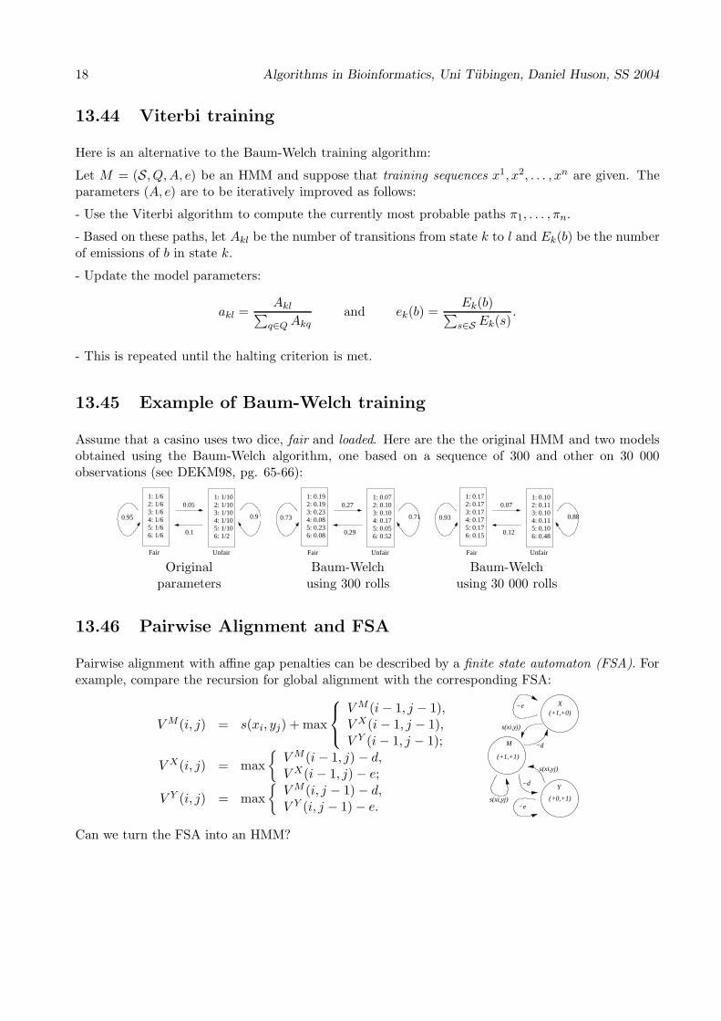
13.45 Example of Baum-Welch training
Assume that a casino uses two dice, fair and loaded. Here are the the original HMM and two modelsobtained using the Baum-Welch algorithm, one based on a sequence of 300 and other on 30 000observations (see DEKM98, pg. 65-66):
1: 1/62: 1/63: 1/64: 1/65: 1/66: 1/6
1: 1/102: 1/103: 1/104: 1/105: 1/106: 1/2
0.05
0.1
0.95 0.9
UnfairFair
1: 0.072: 0.103: 0.104: 0.175: 0.056: 0.52
0.27
0.29
UnfairFair
0.73 0.71
1: 0.192: 0.193: 0.234: 0.085: 0.236: 0.08
3: 0.10
UnfairFair
1: 0.172: 0.173: 0.174: 0.175: 0.176: 0.15
0.93
0.07
0.12
1: 0.102: 0.11
4: 0.115: 0.106: 0.48
0.88
Original Baum-Welch Baum-Welchparameters using 300 rolls using 30 000 rolls
13.46 Pairwise Alignment and FSA
Pairwise alignment with affine gap penalties can be described by a finite state automaton (FSA). Forexample, compare the recursion for global alignment with the corresponding FSA:
VM (i, j) = s(xi, yj) + max
VM (i− 1, j − 1),V X(i− 1, j − 1),V Y (i− 1, j − 1);
V X(i, j) = max
VM (i− 1, j) − d,V X(i− 1, j) − e;
V Y (i, j) = max
VM (i, j − 1)− d,V Y (i, j − 1)− e. (+0,+1)
−es(xi,yj)
−d
s(xi,yj)
(+1,+1)
M −d
s(xi,yj)
−e(+1,+0)
X
Y
Can we turn the FSA into an HMM?

Algorithms in Bioinformatics, Uni Tubingen, Daniel Huson, SS 2004 19
13.47 Pair HMMs
A pair HMM is an HMM that emits pairs of symbols. We obtain a pair HMM from the FSA bymaking two sets of changes. First, we must give probabilities to emissions and transitions:
qyjε
1−2δ
δ
1−ε
Pxiyj
M δ
1−ε
εqxiX
Y
There are two free parameters for transitions between the three main states, δ the probability of atransition from M to X or Y and ǫ, the probability of staying in an insert state (X or Y ).
Second, we must add a begin and end state to provide a probability distribution over all possiblesequences:
qyjε
1−2δ−τ
δ
Pxiyj
M δ
1−ε−τ
εqxiX
Y
τ
τ
τ
τ1−2δ−τ
1−ε−τ
BEGIN END
δ
δ
We assume here that the probability of transitioning into the end state from any other state is τ .
13.48 Viterbi algorithm for pair HMMs
Input: Sequences x = x1 . . . xn and y = y1 . . . ym.Output: Alignment based on most probable pathInit.: Set vM (0, 0) = 1, set all other v·(i, 0), v·(0, j) to 0.For i = 1, . . . , n, j = 1, . . . ,m do:
vM (i, j) = pxiyjmax
(1− 2δ − τ)vM (i− 1, j − 1),(1− ǫ− τ)vX(i− 1, j − 1),(1− ǫ− τ)vY (i− 1, j − 1);
vX(i, j) = qximax
δvM (i− 1, j) − d,ǫvX(i− 1, j) − e;
V Y (i, j) = qyjmax
δvM (i, j − 1)− d,ǫvY (i, j − 1)− e.
Termination:vE = τ max(vM (n,m), vX (n,m), vY (n,m)).

20 Algorithms in Bioinformatics, Uni Tubingen, Daniel Huson, SS 2004
One can show that the most probable path corresponds to an optimal global alignment (in the FSAsense).
13.49 Protein identification
#A-helices ...........AAAAAAAAAAAAAAAA...BBBBBBBBBBBBBBBBCCCCCCCCCCC....DDDDDDDEEEEEEEEEEEE
GLB1_GLYDI .........GLSAAQRQVIAATWKDIAGADNGAGVGKDCLIKFLSAHPQMAAVFG.FSG....AS...DPGVAALGAKVL
HBB_HUMAN ........VHLTPEEKSAVTALWGKV....NVDEVGGEALGRLLVVYPWTQRFFESFGDLSTPDAVMGNPKVKAHGKKVL
HBA_HUMAN .........VLSPADKTNVKAAWGKVGA..HAGEYGAEALERMFLSFPTTKTYFPHF.DLS.....HGSAQVKGHGKKVA
MYG_PHYCA .........VLSEGEWQLVLHVWAKVEA..DVAGHGQDILIRLFKSHPETLEKFDRFKHLKTEAEMKASEDLKKHGVTVL
GLB5_PETMA PIVDTGSVAPLSAAEKTKIRSAWAPVYS..TYETSGVDILVKFFTSTPAAQEFFPKFKGLTTADQLKKSADVRWHAERII
GLB3_CHITP ..........LSADQISTVQASFDKVKG......DPVGILYAVFKADPSIMAKFTQFAG.KDLESIKGTAPFETHANRIV
LGB2_LUPLU ........GALTESQAALVKSSWEEFNA..NIPKHTHRFFILVLEIAPAAKDLFS.FLK.GTSEVPQNNPELQAHAGKVF
#A-helices EEEEEEEEE............FFFFFFFFFFFF..FFGGGGGGGGGGGGGGGGGGG.....HHHHHHHHHHHHHHHHHHH
GLB1_GLYDI AQIGVAVSHL..GDEGKMVAQMKAVGVRHKGYGNKHIKAQYFEPLGASLLSAMEHRIGGKMNAAAKDAWAAAYADISGAL
HBB_HUMAN GAFSDGLAHL...D..NLKGTFATLSELHCDKL..HVDPENFRLLGNVLVCVLAHHFGKEFTPPVQAAYQKVVAGVANAL
HBA_HUMAN DALTNAVAHV...D..DMPNALSALSDLHAHKL..RVDPVNFKLLSHCLLVTLAAHLPAEFTPAVHASLDKFLASVSTVL
MYG_PHYCA TALGAILKK....K.GHHEAELKPLAQSHATKH..KIPIKYLEFISEAIIHVLHSRHPGDFGADAQGAMNKALELFRKDI
GLB5_PETMA NAVNDAVASM..DDTEKMSMKLRDLSGKHAKSF..QVDPQYFKVLAAVIADTVAAG.........DAGFEKLMSMICILL
GLB3_CHITP GFFSKIIGEL..P...NIEADVNTFVASHKPRG...VTHDQLNNFRAGFVSYMKAHT..DFA.GAEAAWGATLDTFFGMI
LGB2_LUPLU KLVYEAAIQLQVTGVVVTDATLKNLGSVHVSKG...VADAHFPVVKEAILKTIKEVVGAKWSEELNSAWTIAYDELAIVI
#A-helices HHHHHHH....
GLB1_GLYDI ISGLQS.....
HBB_HUMAN AHKYH......
HBA_HUMAN TSKYR......
MYG_PHYCA AAKYKELGYQG Alignment of seven Globinsequences
GLB5_PETMA RSAY....... How can this family be characterized?
GLB3_CHITP FSKM.......
LGB2_LUPLU KKEMNDAA...
13.50 Characterization?
How can one characterize a family of protein sequences?
Exemplary sequence?
Consensus sequence?
Regular expression (Prosite):
LGB2_LUPLU ...FNA--NIPKH...
GLB1_GLYDI ...IAGADNGAGV...
...[FI]-[AN]-x(1,2)-N-[IG]-[AP]-[GK]-[HV]...
HMM?
13.51 Simple HMM
HBA_HUMAN ...VGA--HAGEY...
HBB_HUMAN ...V----NVDEV...
MYG_PHYCA ...VEA--DVAGH...
GLB3_CHITP ...VKG------D...

Algorithms in Bioinformatics, Uni Tubingen, Daniel Huson, SS 2004 21
GLB5_PETMA ...VYS--TYETS...
LGB2_LUPLU ...FNA--NIPKH...
GLB1_GLYDI ...IAGADNGAGV...
"Matches": *** *****
We first consider a simple HMM that is equivalent to a PSSM (Position Specific Score Matrix):
ADEGP
AEGKY
VFI
AGS
DHNT
AGIVY
EGKT
HSVY
D
(The listed amino-acids have a higher emission-probability.)
13.52 Insert-states
We introduce so-called insert-states that emit symbols based on their background probabilities.
ADEGP
AEGKY
VFI
AGS
DHNT
AGIVY
EGKT
HSVY
DBegin End
This allows us to model segments of sequence that lie outside of conserved domains.
13.53 Delete-states
We introduce so-called delete-states that are silent and do not emit any symbols.
ADEGP
AEGKY
VFI
AGS
DHNT
AGIVY
EGKT
HSVY
DBegin End
This allows us to model the absence of individual domains.

22 Algorithms in Bioinformatics, Uni Tubingen, Daniel Huson, SS 2004
13.54 Topology of a profile-HMM
Begin End
Match-state, Insert-state, Delete-state
13.55 Design of a profile-HMM
Given a multiple alignment of a family of sequences.
First we must decide which positions are to be modeled as match- and which positions are to bemodeled as insert-states. Rule-of-thumb: columns with more than 50% gaps should be modeled asinsert-states.
We determine the transition and emission probabilities simply by counting the observed transitionsAkl and emissions Ek(B):
akl =Akl
∑
l′ Akl′and ek(b) =
Ek(b)∑
b′ Ek(b′).
Obviously, it may happen that certain transitions or emissions do not appear in the training data andthus we use the Laplace-rule and add 1 to each count.

Algorithms in Bioinformatics, Uni Tubingen, Daniel Huson, SS 2004 19
14 Gene Prediction
This exposition is based on the following sources, which are all recommended reading:
1. Pavel A. Pevzner. Computational Molecular Biology, an algorithmic approach. MIT, 2000,chapter 9.
2. Chris Burge and Samuel Karlin. Prediction of complete gene structures in human genomic DNA.Journal of Molecular Biology, 268:78-94 (1997).
3. Ian Korf, Paul Flicek, Danial Duan and Michael R. Brent, Integrating Genomic Homology intoGene Structure Prediction, Bioinformatics, Vol. 1 Suppl 1., pages S1-S9 (2001).
4. Vineet Bafna and Daniel Huson. The conserved exon method for gene finding. ISMB 2000, 3-12(2000).
5. M. S. Gelfand, A. Mironov and P. A. Pevzner, Gene recognition via spliced alignment, PNAS,93:9061–9066 (1996).
14.1 Introduction
In the 1960s, it was discovered that a gene and its protein product are colinear structures with a directcorrelation between the triplets of nucleotides in the gene and the amino acids in the protein.
It soon became clear that genes can be difficult to determine, due to the existence of overlappinggenes, and genes within genes etc.
Moreover, the paradox arose that the genome size of many eukaryotes does not correspond to “geneticcomplexity”, for example, the salamander genome is 10 times the size of that of human.
In 1977, the surprising discovery of “split” genes was made: genes that consist of multiple pieces ofcoding DNA called exons, separated by stretches of non-coding DNA called introns.
mRNA
DNA
Translation
Transcription
Protein
RNA
splicing
Protein
mRNA
DNA
nucleus
Prokaryote Eukaryote
The existence of split genes and junk-DNA raises a computational gene prediction problem that isstill unsolved:

20 Algorithms in Bioinformatics, Uni Tubingen, Daniel Huson, SS 2004
Given a string of DNA. The gene prediction problem is to reliably predict all genes con-tained in the sequence.
14.2 Three approaches to gene finding
One can distinguish between three types of approaches:
• Statistical or ab initio methods. These methods attempt to predict genes based on statisticalproperties of the given DNA sequence. Programs are e.g. Genscan, GeneID, GENIE andFGENEH.
• Homology methods. The given DNA sequence is compared with known protein structures, e.g.using “spliced alignments”. Programs are e.g. Procrustes and GeneWise.
• Comparative methods. The given DNA string is compared with a similar DNA string froma different species at the appropriate evolutionary distance and genes are predicted in bothsequences based on the assumption that exons will be well conserved, whereas introns will not.Programs are e.g. CEM (conserved exon method) and Twinscan.
14.3 Simplest approach to gene prediction
The simplest way to detect potential coding regions is to look at Open Reading Frames (ORFs). AnORF is a sequence of codons in DNA that starts with a Start codon (ATG), ends with a Stop codon(TAA, TAG or TGA) and has no other (in-frame) stop codons inside.
The average distance between stop codons in “random” DNA is 643 ≈ 21, much smaller than the
number of codons in an average protein (≈ 300).
Essentially, long ORFs indicate genes, whereas short ORF may or may not indicate genes or shortexons.
Additionally, features such as codon usage or hexamer counts can be taken into account. The codonusage of a string of DNA is given by a 64-component vector that counts how many times each codonis present in the string. These values can differ significantly between coding and non-coding DNA.
14.4 Eukaryotic gene structure
For our purposes, a eukaryotic gene has the following structure:
Initialexon
internalexon(s)
Terminalexon
GT GT
Pro
mot
or
5’ U
TR
Sta
rt s
ite
3’ U
TR
Don
or s
ite
Acc
epto
r si
te
ATG TAATAGTGA
AAATAAAA TATA
IntronIntron Sto
p si
te
Poly−A
AG AG

Algorithms in Bioinformatics, Uni Tubingen, Daniel Huson, SS 2004 21
Ab initio gene prediction methods use statistical properties of the different components of such a genemodel to predict genes in unannotated DNA. For example, for the bases around the start site we mayhave the following observed frequencies (given by this position weight matrix):
Pos. -8 -7 -6 -5 -4 -3 -2 -1 +1 +2 +3 +4 +5 +6 +7
A .16 .29 .20 .25 .22 .66 .27 .15 1 0 0 .28 .24 .11 .26
C .48 .31 .21 .33 .56 .05 .50 .58 0 0 0 .16 .29 .24 .40
G .18 .16 .46 .21 .17 .27 .12 .22 0 0 1 .48 .20 .45 .21
T .19 .24 .14 .21 .06 .02 .11 .05 0 1 0 .09 .26 .21 .21
14.5 GENSCAN’s model
We are going to discuss the popular program Genscan in detail, which is based on a semi-Markovmodel:
A+(poly−Asignal)
Einit+(initialexon)
Eterm+(terminal
exon)
F+(5’ UTR)
Esngl+(single−exon
gene)
T+(3’ UTR)
P+(promoter)
N(intergenic
region)
E0+ E1+ E2+
I0+ I1+ I2+
Forward (+) strand
Reverse (−) strand
F−(5’ UTR)
P−(promoter)
Esngl−(single−exon
gene)
A−(poly−Asignal)
Eterm−(terminal
exon)
T−(3’ UTR)
Einit−(initialexon)
E0− E1− E2−
I0− I1− I2−
Genscan’s model can be formulated as an explicit state duration HMM. This is an HMM in which,additionally, a duration period is explicitly modeled for each state, using a probability distribution.The model is thought of generating a parse φ, consisting of:
• a sequence of states q = (q1, q2, . . . , qn), and
• an associated sequence of durations d = (d1, d2, . . . , dn),
which, using probabilistic models for each of the state types, generates a DNA sequence S of lengthL =
∑ni=1 di.
The generation of a parse of a given sequence length L proceeds as follows:
1. An initial state q1 is chosen according to an initial distribution π on the states, i.e. πi = P (q1 =Q(i)), where Q(j) (j = 1, . . . , 27) is an indexing of the states of the model.

22 Algorithms in Bioinformatics, Uni Tubingen, Daniel Huson, SS 2004
2. A state duration or length d1 is generated conditional on the value of q1 = Q(i) from the durationdistribution fQ(i).
3. A sequence segment s1 of length d1 is generated, conditional on d1 and q1, according to anappropriate sequence-generating model for state type q1.
4. The subsequent state q2 is generated, conditional on the value of q1, from the (first-order Markov)state transition matrix T , i.e. Ti,j = P (qk+1 = Q(j) | qk = Q(i)).
This process is repeated until the sum∑n
i=1 di of the state durations first equals or exceeds L, at whichpoint the last state duration is appropriately truncated, the final stretch of sequence is generated andthe process stops.
The resulting sequence is simply the concatenation of the sequence segments, S = s1s2 . . . sn.
Note that the generated sequence is not restricted to correspond to a single gene, but could represent multiple
genes, in both strands, or none.
In addition to its topology involving the 27 states and 46 transitions depicted above, the model hasfour main components:
• a vector of initial probabilities π,
• a matrix of state transition probabilities T ,
• a set of length distributions f , and
• a set of sequence generating models P .
(Recall that an HMM has initial-, transition- and emission probabilities).
14.6 Maximum likelihood prediction
Given such a model M . For a fixed sequence length L, consider
Ω = ΦL × S,
where ΦL is the set of all possible parses of M of length L and SL is the set of all possible sequencesof length L.
The model M assigns a probability density to each point (parse/sequence pair) in Ω. Thus, for a givensequence S ∈ SL, a conditional probability of a particular parse φ ∈ ΦL is given by:
P (φ | S) =P (φ, S)
P (S)=
P (φ, S)∑
φ′∈ΦLP (φ′, S)
,
using P (M,D) = P (M | D)P (D).
The essential idea is to specify a precise probabilistic model of what a gene looks like in advance andthen to select the parse φ through the model M that has highest likelihood, given the sequence S.

Algorithms in Bioinformatics, Uni Tubingen, Daniel Huson, SS 2004 23
14.7 Computational issues
Given a sequence S of length L, the joint probability P (φ, S) of generating the parse φ and thesequence S is given by:
P (φ, S) = πq1fq1(d1)P (s1 | q1, d1)
×n∏
k=2
Tqk−1,qkfqk
(dk)P (sk | qk, dk),
where the states of φ are q1, q2, . . . , qn with associated state lengths d1, d2, . . . , dn, which break thesequence into segments s1, s2, . . . , sn.
Here, P (sk | qk, dk) is the probability of generating the segment sk under the appropriate sequencegenerating model for a type-qk state of length dk.
A modification of the Viterbi algorithm may be used to calculate φopt, the parse with maximal jointprobability (under M), that gives the predicted gene or set of genes in the sequence.
We can compute P (S) using the “forward algorithm” discussed under HMMs. With the help of the“backward algorithm”, certain additional quantities of interest can also be computed.
For example, consider the event E(k)[x,y] that a particular sequence segment [x, y] is an internal exon of
phase k ∈ 0, 1, 2. Under M , this event has probability
P (E(k)[x,y] | S) =
∑
φ:E(k)[x,y]
∈φP (φ, S)
P (S),
where the sum is taken over all parses that contain the given exon E(k)[x,y]. This sum can be computed
using the forward and backward algorithms.
14.8 Details of the model
So far, we have discussed the topology and the other main components of the Genscan model ingeneral terms. The following details need to be discussed:
• the initial and transition probabilities,
• the state length distributions,
• transcriptional and translational signals,
• splice signals, and
• reverse-strand states.

24 Algorithms in Bioinformatics, Uni Tubingen, Daniel Huson, SS 2004
14.9 Initial and transition probabilities
For gene prediction in randomly chosen blocks of contiguous human DNA, the initial probability ofeach state should be chosen proportionally to its estimated frequency in bulk human genomic DNA.
This is a non-trivial problem, because gene density and certain aspects of gene structure vary signifi-cantly in regions of differing C+G content (so-called “isochores”) of the human genome, with a muchhigher gene density in C+G-rich regions.
Hence, in practice, initial and transitional probabilities are estimated for four different categories:(I) < 43% C+G, (II) 43− 51% C+G, (III) 51 − 57% C+G, and (IV) > 57% C+G.
The following initial probabilities were obtained from a training set of 380 genes by comparing thenumber of bases corresponding to each of the different states:
Group I II III IVC+G-range < 43% 43− 51% 51− 57% > 57%Initial probabilities:Intergenic (N) 0.892 0.867 0.540 0.418Intron (I+
i , I−i ) 0.095 0.103 0.338 0.388
5’ UTR (F+, F−) 0.008 0.018 0.077 0.1223’ UTR (T+, T−) 0.005 0.011 0.045 0.072
For simplicity, the initial probabilities for the exon, promoter and poly-A states were set to 0.
Transition probabilities are obtained in a similar way.
14.10 State length distributions
In general, the states of the model correspond to sequence segments of highly variable length.
For certain states, most notably for internal exon states Ek, length is probably important for properbiological function, i.e. proper splicing and inclusion in the final processed mRNA.
For example, it has been shown in vivo that internal deletions of exons to sizes below about 50 bp mayoften lead to exon skipping, and there is evidence that steric interference between factors recognizingsplice sites may make splicing of small exons more difficult. There is also evidence that spliceosomalassembly is inhibited if internal exons are expanded beyond 300 bp.
In summary, these arguments support the observation that internal exons are usually ≈ 120− 150 bplong, with only a few of length less that 50 bp or more than 300 bp.
Constraints for initial and terminal exons are slightly different.
The duration in initial, internal and terminal exon states is modeled by a different empirical distribu-tion for each of the types of states.
In contrast to exons, the length of introns does not seem critical, although a minimum length of 70−80may be preferred.
The length distribution for introns appears to be approximately geometric (exponential). However,the average length of introns differs substantially between the different C+G groups: In group I, theaverage length is 2069 bp, whereas for group IV , the average length is only 518 bp.

Algorithms in Bioinformatics, Uni Tubingen, Daniel Huson, SS 2004 25
Hence, the duration in intron states is modeled by a geometric distribution with parameter q estimatedfor each C+G group separately.
Empirical length distributions for introns and exons:
2k 3k 4k 6k0 1k 5k 7k 8k
0
100
200
300
Length (bp)
Num
ber
of in
tron
s
0
0
Length (bp)
200 400
Num
ber
of e
xons
30
60
75
Introns Initial exons
0
0
Length (bp)
100
200
250
200 400
Num
ber
of e
xons
0
0
Length (bp)
200 400
Num
ber
of e
xons
40
20
Internal exons Terminal exons
Note that the exon lengths generated must be consistent with the phases of adjacent introns. Toaccount for this, first the number of complete codons is generated from the appropriate length distri-bution, then the appropriate number (0, 1 or 2) of bp is added to each end to account for the phasesof the preceding and subsequent states.
For example, if the number of complete codons generated for an internal exon is C = 6, and thephase of the previous and next intron is 1 and 2, respectively, then the total length of the exon isl = 3C + 2 + 2 = 22:
phase 1 intron phase 2 intronexon
TA CGC GCT CGC TTACTGTTTGT
For the 5′ UTR and 3′ UTR states, geometric distributions are used with mean values of 769 and457 bp, respectively.
14.11 Simple signal models
There are a number of different models of biological signal sequences, such as donor and acceptor sites,promoters, etc.
One of the earliest and must influential approaches is the weight matrix method (WMM), in which the
frequency p(i)a of each nucleotide a at position i of a signal of length n is derived from a collection of
aligned signal sequences.
The product P (A) =∏n
i=1 P(i)ai is used to estimate the probability of generating a particular sequence
A = a1a2 . . . an.
26 Algorithms in Bioinformatics, Uni Tubingen, Daniel Huson, SS 2004
The weight array matrix (WAM) is a generalization that takes dependencies between adjacent po-sitions into account. In this model, the probability of generating a particular sequence is P (A) =
p(1)a1
∏ni=2 p
i−1,iai−1,ai , where pi−1,i
v,w is the conditional probability of generating a particular nucleotide w atposition i, given nucleotide v at position i− 1.
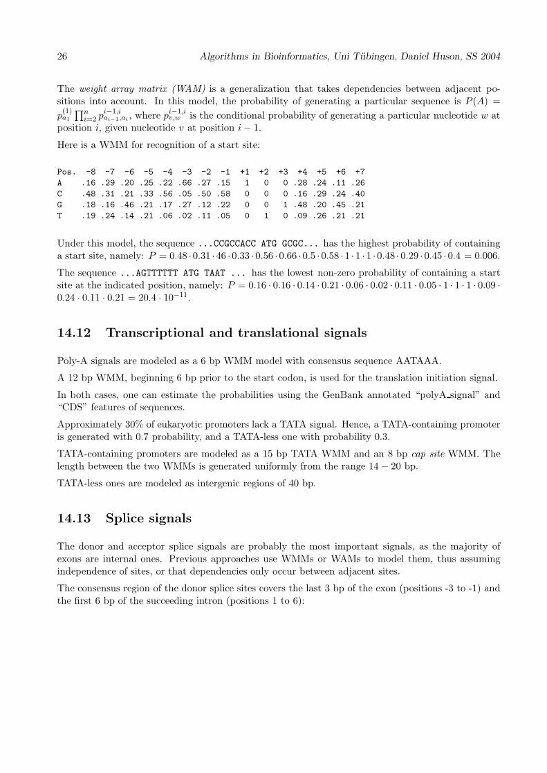
Here is a WMM for recognition of a start site:
Pos. -8 -7 -6 -5 -4 -3 -2 -1 +1 +2 +3 +4 +5 +6 +7
A .16 .29 .20 .25 .22 .66 .27 .15 1 0 0 .28 .24 .11 .26
C .48 .31 .21 .33 .56 .05 .50 .58 0 0 0 .16 .29 .24 .40
G .18 .16 .46 .21 .17 .27 .12 .22 0 0 1 .48 .20 .45 .21
T .19 .24 .14 .21 .06 .02 .11 .05 0 1 0 .09 .26 .21 .21
Under this model, the sequence ...CCGCCACC ATG GCGC... has the highest probability of containinga start site, namely: P = 0.48 ·0.31 ·46 ·0.33 · 0.56 · 0.66 · 0.5 · 0.58 · 1 · 1 · 1 ·0.48 · 0.29 · 0.45 · 0.4 = 0.006.
The sequence ...AGTTTTTT ATG TAAT ... has the lowest non-zero probability of containing a startsite at the indicated position, namely: P = 0.16 · 0.16 · 0.14 · 0.21 · 0.06 · 0.02 · 0.11 · 0.05 · 1 · 1 · 1 · 0.09 ·0.24 · 0.11 · 0.21 = 20.4 · 10−11.
14.12 Transcriptional and translational signals
Poly-A signals are modeled as a 6 bp WMM model with consensus sequence AATAAA.
A 12 bp WMM, beginning 6 bp prior to the start codon, is used for the translation initiation signal.
In both cases, one can estimate the probabilities using the GenBank annotated “polyA signal” and“CDS” features of sequences.
Approximately 30% of eukaryotic promoters lack a TATA signal. Hence, a TATA-containing promoteris generated with 0.7 probability, and a TATA-less one with probability 0.3.
TATA-containing promoters are modeled as a 15 bp TATA WMM and an 8 bp cap site WMM. Thelength between the two WMMs is generated uniformly from the range 14− 20 bp.
TATA-less ones are modeled as intergenic regions of 40 bp.
14.13 Splice signals
The donor and acceptor splice signals are probably the most important signals, as the majority ofexons are internal ones. Previous approaches use WMMs or WAMs to model them, thus assumingindependence of sites, or that dependencies only occur between adjacent sites.
The consensus region of the donor splice sites covers the last 3 bp of the exon (positions -3 to -1) andthe first 6 bp of the succeeding intron (positions 1 to 6):

Algorithms in Bioinformatics, Uni Tubingen, Daniel Huson, SS 2004 27
. . . exon intron. . .Position -3 -2 -1 +1 +2 +3 +4 +5 +6Consensus c/a A G G T a/g A G tWMM:A .33 .60 .08 0 0 .49 .71 .06 .15C .37 .13 .04 0 0 .03 .07 .05 .19G .18 .14 .81 1 0 .45 .12 .84 .20T .12 .13 .07 0 1 .03 .09 .05 .46
14.14 Donor site model
However, donor sites show significant dependencies between non-adjacent positions, which probablyreflect details of donor splice site recognition by U1 snRNA and other factors.
Given a sequence S. Let Ci denote the consensus indicator variable that is 1, if the given nucleotideat position i matches the consensus at position i, and 0 otherwise. Let Xj denote the nucleotide atposition j.
For example, consider:
. . . exon intron. . .Position -3 -2 -1 +1 +2 +3 +4 +5 +6Consensus c/a A G G T a/g A G tS . . . T A A C G T A A G C C . . .
Here, C−1 = 0 and C+6 = 0, and = 1, for all other positions. Similarly, X−3 = A, X−2 = A, X−1 = Cetc.
For each pair of positions i 6= j, consider the Ci versus Xj contingency table computed from the givenlearning set of gene structures:
Xj
Ci A C G T
0 f0(A) f0(C) f0(G) f0(T )1 f1(A) f1(C) f1(G) f1(T ),
where fc(x) is the frequency at which the training set has the consensus indicator value c at positioni and the base x at position j. The (Pearson’s) χ2-test assigns a score χ2(Ci,Xj) to each pair ofvariables Ci and Xj :
χ2(Ci,Xj) =∑
c∈0,1
∑
x∈A,C,G,T
(fc(x)− f(x)
f(x)
)2
,
where f(x) denotes the frequency with which we observe Xj = x in the training set (corresponding tothe null-hypothesis that Xj does not depend on Ci).
A significant score indicates that a dependency exists between Ci and Xj.
In donor site prediction, the positions i are ordered by decreasing discriminatory power Zi =∑
j 6=i χ2(Ci,Xj) and separate WMMs for each of the different cases are derived, thus obtaining a
so-called maximal dependence decomposition:

28 Algorithms in Bioinformatics, Uni Tubingen, Daniel Huson, SS 2004
(Source: Burge and Karlin 1997)
Here, H = A|C|U , B = C|G|U and V = A|C|G. For example, G5 , or H5, is the set of donor sites with, or
without, a G at position +5, respectively.
14.15 Acceptor site model
Intron/exon junctions are modeled by a (first-order) WAM for bases −20 to +3, capturing the pyrim-idine (C,T) rich region and the acceptor splice site itself.
It is difficult to model the branch point in the preceding intron, and only 30% of the test data had anYYRAY sequence in the appropriate region [−40,−21].
A modified variant of a second-order WAM is employed in which nucleotides are generated conditionalon the previous two ones, in an attempt to model the weak but detectable tendency toward YYYtriplets as well as certain branch point-related triplets such as TGA, TAA, GAC, and AAC in thisregion, without requiring the occurrence of any specific branch point consensus.
(A windowing and averaging process is used to obtain estimates from the limited training data.)
14.16 Exon models
Coding portions of exons are modeled using an inhomogeneous 3-periodic fifth order Markov model.Here, separate Markov transition matrices, c1, c2 and c3, are determined for hexamers ending at eachof the three codon positions, respectively:

Algorithms in Bioinformatics, Uni Tubingen, Daniel Huson, SS 2004 29
xxxxxxxxxx xxxxxxxxxxx1 x2 x3 y1 y2 y3 z1 z2 z3
C2
C1
C3
This is based on the observation that frame-shifted hexamer counts are generally the most accuratecompositional discriminator of coding versus non-coding regions.
However, A+T rich genes are often not well predicted using hexamer counts based on bulk DNA andso Genscan uses two different sets of transition matrices, one trained for sequences with < 43% C+Gcontent and one for all others.
14.17 Example of Genscan summary output
GENSCAN 1.0 Date run: 28-Apr-104 Time: 02:56:56
Sequence HUMAN DNA : 36741 bp : 52.90% C+G : Isochore 3 (51 - 57 C+G%)
Parameter matrix: HumanIso.smat
Predicted genes/exons:
Gn.Ex Type S .Begin ...End .Len Fr Ph I/Ac Do/T CodRg P.... Tscr..
----- ---- - ------ ------ ---- -- -- ---- ---- ----- ----- ------
1.01 Intr + 3420 3538 119 1 2 104 66 32 0.106 3.29
1.02 Intr + 3950 4063 114 1 0 22 61 133 0.276 5.15
1.03 Term + 4310 4426 117 1 0 83 44 64 0.725 0.34
1.04 PlyA + 5029 5034 6 1.05
2.05 PlyA - 5519 5514 6 1.05
2.04 Term - 7619 7455 165 2 0 36 47 124 0.792 1.33
2.03 Intr - 9364 9309 56 2 2 90 84 48 0.603 3.79
2.02 Intr - 9557 9478 80 1 2 70 53 49 0.904 -0.71
2.01 Init - 9986 9910 77 2 2 90 90 58 0.701 6.79
2.00 Prom - 13449 13410 40 -3.91
3.02 PlyA - 14233 14228 6 -0.45
3.01 Sngl - 14748 14287 462 0 0 13 51 222 0.425 7.51
3.00 Prom - 17109 17070 40 -7.00
4.00 Prom + 19924 19963 40 0.29
...
14.18 Performance studies
The performance of a gene prediction program is evaluated by applying it to DNA sequences for whichall contained genes are known and annotated with high confidence.
To calculate accuracy statistics, each nucleotide of a test sequence is classified as:
• a predicted positive (PP) if it is predicted to be contained in a coding region,
30 Algorithms in Bioinformatics, Uni Tubingen, Daniel Huson, SS 2004
• a predicted negative (PN) if it is predicted to be contained in non-coding region,
• an actual positive (AP) if it is annotated to be contained in coding region, and
• an actual negative (AN) if it is annotated to be contained in non-coding region.
The performance is measured both on the level of nucleotides and on whole predicted exons, using asimilar classification.
Based on this classification, we compute the number of:
• true positives, TP = PP ∩AP ,
• false positives, FP = PP ∩AN ,
• true negatives, TN = PN ∩AN , and
• false negatives, FN = PN ∩AP .
The sensitivity Sn and specificity Sp of a method are then defined as
Sn =TP
APand Sp =
TP
PP,
respectively, measuring both the ability to predict true genes and to avoid predicting false ones.
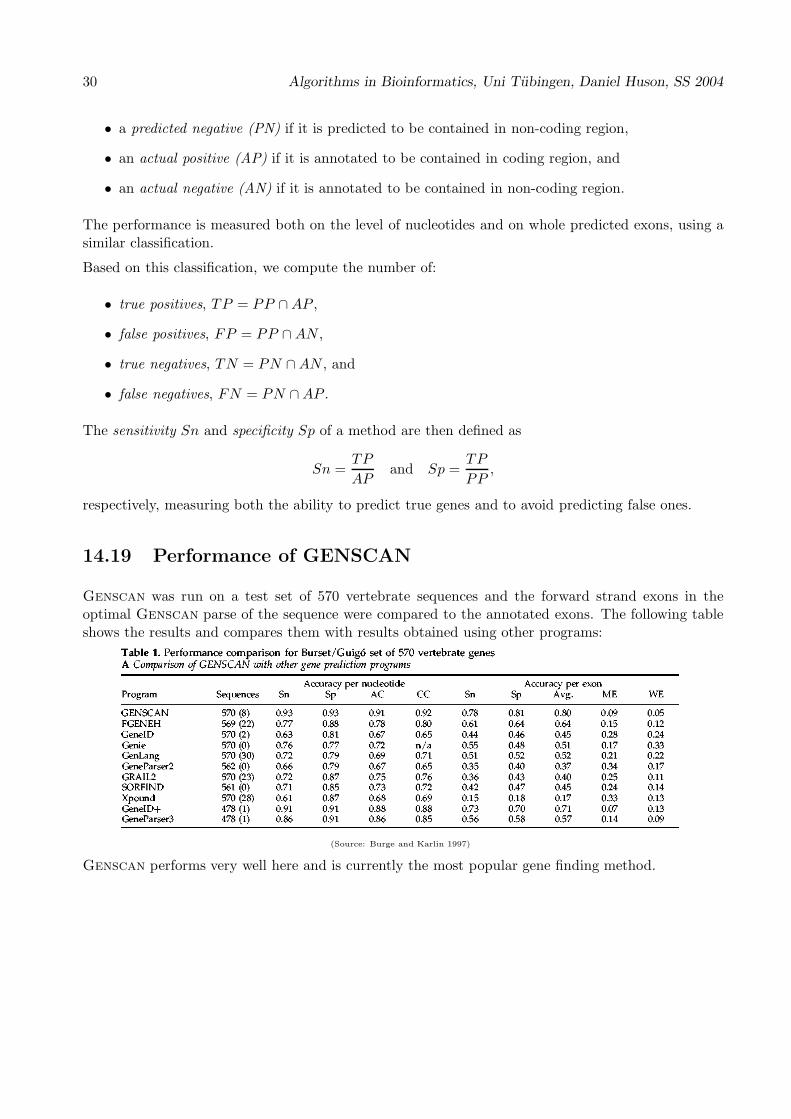
14.19 Performance of GENSCAN
Genscan was run on a test set of 570 vertebrate sequences and the forward strand exons in theoptimal Genscan parse of the sequence were compared to the annotated exons. The following tableshows the results and compares them with results obtained using other programs:
(Source: Burge and Karlin 1997)
Genscan performs very well here and is currently the most popular gene finding method.

Algorithms in Bioinformatics, Uni Tubingen, Daniel Huson, SS 2004 31
14.20 Comparative gene finding
Genscan’s model makes use of statistical features of the genome under consideration, obtained froman annotated training set.
More recently, a number of methods have been suggested that attempt to also make use of comparativedata. They are based on the observation that
the level of sequence conservation between two species depends on the function of theDNA, e.g. coding sequence is more conserved than intergenic sequence.
One such program is Rosetta, which first computes a global alignment of two homologous sequencesand then attempts to predict genes in both sequences simultaneously. A second is the conserved exonmethod, that uses local conservation.
The Twinscan program is an extension of Genscan, that additionally models a conserved sequence.
14.21 TWINSCAN
The input to Twinscan consists of a target sequence, i.e. a genomic sequence in which genes are tobe predicted, and an informant sequence, i.e. a genomic sequence from a related organism.
For example, the target may come from the mouse genome and the informant from the whole humangenome.
Given a target and an informant, in a preprocessing step, one determines a set of top homologs (e.g.using BLAST) from the informant sequence, i.e. one or more sequences from the informant sequencethat best match the target sequence.
mouse
conserved human (top homologs)
The top homologs represent the regions of conserved informant sequence, which we will simply call“the informant sequence” in the following.
14.22 Conservation sequence
Similarity is represented by a conservation sequence, which pairs one of three symbols with eachnucleotide of the target:
. unaligned | matched : mismatched
Gaps in the informant sequence become mismatch symbols, gaps in the target sequence are ignored.Consider:
123456789 position
GAATTCCGT target sequence

32 Algorithms in Bioinformatics, Uni Tubingen, Daniel Huson, SS 2004
and suppose that BLAST The conservation sequenceyields the following HSP: derived from this HSP is:
345 6789 target position 123456789 position
ATT-CCGT target alignment GAATTCCGT target sequence
|| || | BLAST alignment ..||:||:| conservation sequence
ATCACC-T Informant alignment
The following algorithm takes a list of HSPs and computes the conservation sequence C:
AlgorithmInput: target sequence, list of HSPsOutput: conservation sequence CInit.: C[1..n] := unalignedSort HSPs by alignment scorefor each position i in the target sequence:
for each HSP H from best to worst:if H covers position i:
if C[i] = unaligned:C[i] :=′ |′, in case of a match, and C[i] :=′:′ otherwise
end
Note that the conservation symbol assigned to the target nucleotide at position i is determined by thebest HSP that covers i, regardless of which homologous sequence it comes from. Position i is classifiedas unaligned only if none of the HSPs overlap it.
14.23 Probability of sequence and conservation sequence
Recall that Genscan assigns each nucleotide of an input sequence to one of seven categories: promoter,5’ UTR, exon, intron, 3’ UTR, poly-A signal and intergenic.
Genscan chooses the most likely assignment of categories to nucleotides according to the Genscan
model, using an optimization algorithm (that is, a modification of the Viterbi algorithm).
Given a sequence, the Genscan model assigns a probability to each parse of the sequence (that is, apath of states and durations through the model that generates the sequence.)
The Twinscan model assigns a probability to any parsed DNA sequence together with a parallelconservation sequence. Under this model, the probability of a DNA sequence and the probability ofthe parallel conservation sequence are independent, given the parse.
Consider the following example:
10 20 30
123456789|123456789|123456789|123456789
ATTTAGCCTACTGAAATGGACCGCTTCAGCATGGTATCC target sequence T
||:|||.........|:|:|||||||||:||:|||::|| conservation sequence C

Algorithms in Bioinformatics, Uni Tubingen, Daniel Huson, SS 2004 33
What is the probability of observing the target sequence T7,33 and conservation sequence C7,33 ex-tending from position 7 to 33, given the hypothesis E7,33 that an internal exon extends from position7 to 33?
This is simply the probability of the target sequence T7,33 under the Genscan model times theprobability of the conservation sequence C7,33 under the conservation model, assuming the parseE7,33:
P (T7,33, C7,33 | E7,33) = P (T7,33 | E7,33)P (C7,33 | E7,33).
14.24 TWINSCAN’s model
Twinscan consists of a new, joint probability model on DNA sequences and conservation sequences,together with the same optimization algorithm used by Genscan.
Twinscan augments the state-specific sequence models of Genscan with models for the probabilityof generating any given conservation sequence from any given state.
Coding, UTR, and intron/intergenic states all assign probabilities to stretches of conservation sequenceusing homogeneous 5th-order Markov chains:
c1 c2 c3 c4 c5 c6ccccccccccc cccccccccccOne set of parameters is estimated for each of these types of regions.
Again, consider:
10 20 30
123456789|123456789|123456789|123456789
ATTTAGCCTACTGAAATGGACCGCTTCAGCATGGTATCC target sequence T
||:|||.........|:|:|||||||||:||:|||::|| conservation sequence C
The probability of observing C7,33, given E7,33, is:
PC(C7,33 | E7,33) = PE(C7,7 | C2,6) · . . . · PE(C33,33 | C28,32),
where PE(C33,33 | C28,32), for example, is the estimated probability of a ‘|’ (match) following the givecontext symbols “|:||:” in the conservation sequence of an exon.
Models of conservation at splice donor and acceptor sites are modeled using 2nd-order WAMs of length9 bp and 43 bp, respectively (lengths as in Genscan).
14.25 TWINSCAN’s performance
Twinscan was tested on two data sets. The first set consists of 86 mouse sequences totaling 7.6 Mband used top homologs from human:

34 Algorithms in Bioinformatics, Uni Tubingen, Daniel Huson, SS 2004
Program Exons Exon Sn Exon Sp Genes Genes Sn Genes SpAnnotation 2758 275Genscan 2997 0.631 0.581 395 0.153 0.106Twinscan 2854 0.683 0.660 464 0.244 0.144
The second set is a subset containing 8 pairs of finished orthologs:
Program Exons Exon Sn Exon Sp Genes Genes Sn Genes SpAnnotation 610 48Genscan 731 0.798 0.666 51 0.167 0.157Twinscan 684 0.854 0.752 50 0.271 0.260
14.26 The conserved exon method (CEM)
Based on a model of sequence conservation, Twinscan uses an informant sequence to obtain bettergene predictions for a given target sequence.
Input to the conserved exon method (CEM) are two related sequences and the method predicts genestructures in both sequences simultaneously. The underlying assumption is that exons are well pre-served, whereas introns and intergenic DNA have very little similarity.
For this assumption to hold, the two input sequences must be at an appropriate evolutionary distance.Coding regions are generally well conserved in species as far back as 450 Myrs. At evolutionarydistances of 50–100 Myrs (human and mouse), the conservation also extends to other functionalregions important for gene expression and maintaining genome structure.
The main idea of CEM is to look for conserved protein sequences by comparing pairs of DNA sequences,to identify putative exons based on sequence and splice site conservation, and then to chain such pairsof conserved exons together to obtain gene structure predictions in both sequences.
Identifying conserved coding sequence The first part of the CEM is not new. For example, thetBLASTx program performs precisely this task. Additionally, a number of tools exist for comparingtwo genomic sequences, finding conserved exons and regulatory regions etc.
Building gene models The second part of the CEM is more interesting, in which gene structuresare generated from the identified matches and complete gene structures are predicted in both inputsequences.
14.27 Application of tBLASTx
Throughout the following, we are given two similar DNA sequences S and T .
The program tBLASTx produces a list of high-scoring pairs (HSPs) of locally aligned substrings ofS and T , where the two substrings are interpreted as amino-acid coding strings and the score of thealignment is computed using a BLOSSUM or PAM protein scoring matrix.
This is how an HSP is reported by tBLASTx:
Score = 214 (98.4 bits), Expect = 0.0, Sum P(24) = 0.0
Identities = 44/46 (95%), Positives = 46/46 (100%), Frame = +1 / +1

Algorithms in Bioinformatics, Uni Tubingen, Daniel Huson, SS 2004 35
Query: 5284 RLVLRIATDDSKAVCRLSVKFGATLRTSRLLLERAKELNIDVVGVR 5421
RLVLRIATDDSKAVCRLSVKFGATL+TSRLLLERAKELNIDV+GVR
Sbjct: 3871 RLVLRIATDDSKAVCRLSVKFGATLKTSRLLLERAKELNIDVIGVR 4008
In this example, the positions 5284–5421 of sequence S and positions 3871–4008 of sequence T arealigned together and interpreted as amino-acids as shown. The “frame” indicates the directions andthe offsets of the two substrings.
tBLASTx matches between two similar pieces of human and mouse DNA:
1000 2000 3000 4000 5000 6000 7000
1000
2000
3000
4000
5000
6000
7000
8000
9000
mus.mask
hum.mask
CEMexplorer: /home/huson/genomics/CG/testcases/J03733_X16277: mus.mask vs. hum.maskornithine_1(+,+)tblastx
14.28 Key assumption for conserved exons
Note that programs such as tBLASTx predict putative coding regions, but not actual splice bound-aries. Also, many HSPs are due to other conserved features, not exons.
In the CEM, the local alignments produced by tBLASTx are used as seeds for dynamic programmingalignments that are computed to detect complete exons.
Key assumption Any pair of conserved exons E1 (in S) and E2 (in T ) possesses a witness, that is,an HSP h whose middle codon is a portion of the correct local alignment of E1 and E2, in the correctframe.
E2
E1A
B
h

36 Algorithms in Bioinformatics, Uni Tubingen, Daniel Huson, SS 2004
14.29 Conserved exon pairs
A putative conserved exon pair (CEP) consists of a pair of substrings E1 (in S) and E2 (in T ) thatare both flanked by appropriate splice junctions and have a high scoring local amino-acid alignment.We now discuss how to obtain putative CEPs.
Given an HSP h. Let mS(h) and mT (h) denote the position of the middle codon of h in S and in T ,respectively.
Let bS(h) and eS(h) denote the position of the left-most possible intron-exon splice site and right-mostpossible exon-intron splice site for any putative exon in S that is witnessed by h. Define bT (h) andeT (h) in the same way.
In a simple approach, we use empirical bounds on the lengths of exons to find the values of bS , eS , bTand eT . A more sophisticated approach takes the amount of coverage by HSPs etc. into account.
Start, stop and splice sites are detected by WMMs or more advanced techniques.
If the values of bS, eS , bT and eT were chosen large enough, then the key assumption implies that thetwo exons E1 (in S) and E2 (in T ) of the true CEP (witnessed by h) will start in [bS(h),mS(h)] and[bT (h),mT (h)], and will end in [mS(h), eS(h)] and [mT (h), eT (h)], respectively.
We evaluate all possible pairs of exons in this region by running two dynamic programs: one starts at(mS(h),mT (h)) and ends at (eS(h), eT (h)), the other runs in reverse direction from (mS(h),mT (h))to (bS(h), bT (h)):
(h)bS
h
(h)
(h)(h)
e
beT
T
S(h)
Sm
(h)mT
14.30 Exon alignment
The actual algorithms used for the local alignment computations are variants of the standard algo-rithm.
Note that the alignments are forced to start in the frame defined by the HSP. Frame-shifts are allowedsubsequently (with an appropriate indel penalty).
Each splice-junction pair is a cell in the dynamic programming matrix, and its score is maintained ina separate list.
Let (i, j) be the coordinates of a cell corresponding to a splice-pair (zS(h), zT (h)). The score assignedto (zS(h), zT (h)) is not Score[i, j], but
Score(zS(h), zT (h)) = max0≤kS(h),kT (h)≤2
Score[i− kS(h)][j − kT (h)]

Algorithms in Bioinformatics, Uni Tubingen, Daniel Huson, SS 2004 37
This is to allow for the possibility of an intron splitting a codon. In this way, the alignment (whichonly scores codons) allows terminal nucleotide gaps without incurring a frame-shift penalty.
The amount of overhang
(oS(h), oT (h)) = arg max0≤kS(h),kT (h)≤2
Score[i− kS(h)][j − kT (h)]
is also stored along with the score.
As the alignment is done at the protein level, there is a direction associated with it. The dynamicprogramming computation from the mid-point to the acceptor splice junctions is done by reversingeach codon before scoring.
14.31 The CEP gadget
For each HSP h we construct a CEP gadget. Each node u in the CEP gadget corresponds to acoordinate pair (i, j), which is the starting point, mid-point or terminating point of a candidate exonpair (E1, E2). More precisely, u is one of the following:
• a center node, if (i, j) = (mS(h),mT (h)) is the position of the middle codon of h,
• a donor node if i ∈ [mS(h), eS(h)] & j ∈ [mT (h), eT (h)] are sites of donor splice signals in S,and T ,
• an acceptor node if i ∈ [bS(h),mS(h)] and j ∈ [bT (h),mT (h)] are sites of acceptor signals,
• a start node if i ∈ [bS(h),mS(h)] and j ∈ [bT (h),mT (h)] are sites of translation initiation signals,or
• a terminal node if i ∈ [mS(h), eS(h)] and j ∈ [mT (h), eT (h)] are sites for a stop codon.
(h)bS
h
(h)
(h)(h)
e
beT
T
S(h)
Sm
(h)mT
→ h
Each node u has some additional information associated with it. The coordinates of the cell aremaintained as (uS , uT ). For each acceptor or donor node u, we maintain information on the nucleotideoverhang at the boundary as overhang(u) = (oS(u), oT (u)).
A directed edge is constructed from each acceptor or start node to the center, and from the center toeach donor or terminal node. The weight of the edge is the score of the corresponding local alignment.

38 Algorithms in Bioinformatics, Uni Tubingen, Daniel Huson, SS 2004
14.32 The CEM graph
As discussed above, each HSP gives rise to a CEP gadget. (In practice, however, different HSPs oftenlead to the same CEP gadget and such redundancies should be removed.)
Each CEP gadget is a concise representation of alignments of pairs of exons. At most one pair canactually be a conserved-exon-pair in the true gene structures. The Conserved-Exon-Method takes allCEP gadgets of HSPs and chains them together, thus obtaining the full “CEM graph”. It builds genemodels from this graph based on the assumption that the transcripts derived from correct orthologousgene structures will have the highest alignment score.
Let S and T be the two genomic sequences.
For each HSP h, compute the CEP gadget. We build a candidate exon graph G = (V,E) (which wecall the CEM graph), as follows: V is the union of all the nodes in the CEP gadgets, and E containsall the edges in each CEP gadget. Further, add an edge from donor or terminal node u to an acceptoror start node v if both:
• vS ≥ uS +M , and vT ≥ uT +M , where M is a suitably chosen minimum intron length, and:
• Let (oS(u), oT (u)) = overhang(u), and (oS(v), oT (v)) = overhang(v). Then, (oS(u) + oS(v)) =0(mod 3), and (oT (u) + oT (v)) = 0(mod 3),
The weight of the edge (u, v) is the score of aligning the amino-acids obtained by concatenating theoverhangs on either side added to the penalty for an intron gap.
Example of linking two CEPs, nodes are labeled by their offsets (oS , oT ):
h
h’(1,2)
(0,1)
(0,0)
(0,0)
(0,2)
(0,2)
(0,0)additio
nal edges l
inking C
EPs
Example of a complete graph:

Algorithms in Bioinformatics, Uni Tubingen, Daniel Huson, SS 2004 39
2.843.1
58.3450.716.3561.3765.657.9654.11
96.67
56.5352.4186.9621.9894.2597.38
20.3686.5782.4178.5762.0252.640.1462.6358.7942.2432.8262.4
23.6553.11
4.2313.5430.0449.8258.1135.1754.9552.98
23.5949.1127.04105.38 89.8879.6282.38
82.8989.6776.6318.7256.7249.76 94.9729.9415.179.41
108.26109.7
165.55155.23145.39114.83
170.68150.1140.26
51.0555.76
6.84
-24-24-32-32-32-32-37
-43
-75-75-74-74
-92-92-99
000
-12-12
-35-35-44-44
000
-12-12
-35-35-44-44
00
-3-3
-26-26-35-35
65656
5
-22-22-22-22
-39-39-46
65656
5
-22-22-22-22
-39-39-46
45
-14-14-16-16
-31-31-38
-20
45
-14-14-16-16
-31-31-38
-20
00
-6-6-15-15
-1-1-10-10
-1-1-10-10
655
-311
64444
-311
6444400
5521111-900
1111-900
1815,23821811,23781825,2392
2917,41442863,40902847,40732832,40732964,41912923,41502863,40902847,40732832,40732964,4191
3293,45713197,45033197,44753370,4648
3557,48983514,48553628,49693590,49313514,48553628,49693589,49303514,48553690,50313686,50273592,49333514,48553690,50313686,5027
3940,53533924,53373873,52864011,54244007,54204002,54204000,54203958,53713924,53373873,52864011,54244007,54204002,54204000,5420
4149,55914109,55514034,54784250,56864190,56324364,58224351,58094438,58754393,58514369,58274351,58094434,58924396,58544369,58274351,58094434,5892
5008,69774979,69485049,70185032,70015057,70264979,69485185,71545170,71105165,71105156,71105141,71105063,70324979,69485185,71545170,71105165,71105156,71105141,71105282,72525223,71935359,73295335,73055314,73055314,7284
5509,74905453,74345418,73995616,75975523,75045519,75005524,75055453,74345453,73995418,73995616,75975523,75045453,74345418,73995636,76175632,76135526,75075453,74345418,73995636,76175632,7613
6205,83096150,82546294,83986238,83426150,82546294,8398
6509,86206505,86166601,8703
14.33 Obtaining a gene prediction
By construction, a path in the CEM graph corresponds to a prediction of orthologous gene structuresin the two genomes. Based on the assumption that the correct gene models will have the highestalignment score, we can extract the correct gene structures simply by choosing the highest-scoringpath. As this is a directed acyclic graph, the highest-scoring path can be computed via a topologicalsort:
getGeneModelScores(CEMGraph G(V,E))begin
OrderedNodeListL = TopologicalSort(G)for each v in L
Initialize(Score(v))for each incoming edge e = (x, v)
if (Score(v) < Score(x) + w(e))Score(v) = Score(x) + w(e)predecessor(v) = x
end
(An ordering φ of the nodes of an acyclic graph is a topological sorting if for any edge (v,w) we haveφ(v) < φ(w).)
For an arbitrary node u, score(u) is the best score of an alignment of two sequence prefixes S[1..ui],and T [1..uj ], allowing for frame-shifts, amino-acid indels and intron penalties.
Once the scores on the nodes are computed, the gene models are built by starting at the node withthe highest score, and following the predecessors. The coordinates of start-, terminal-, donor- and

40 Algorithms in Bioinformatics, Uni Tubingen, Daniel Huson, SS 2004
acceptor nodes reveal the gene structure in the two genomic sequences. As the boundaries of the pathare not limited to start and terminal nodes, partial gene structures can be predicted.
14.34 Multiple genes
Additionally, we add an edge from every stop node v with coordinates (vS , vT ) to every downstreamstart node w (with coordinates wS > vS and wT > vT ). Such edges are given weight 0. The role ofsuch edges is to allow prediction of multiple genes.
HSPs with negative frames in one or both sequences are possible witnesses for exons in the reversestrand of one or both sequences. The CEP gadgets derived from such HSPs are simply added to theCEM graph.
To enable a prediction of genes in both strands simultaneously, appropriate additional edges must beinserted between the start and stop nodes of the CEPs. For example, a stop node obtained from anHSP with +/+ frame is connected to all downstream stop nodes that have frame −/−.
14.35 Summary of CEM algorithm
1. Compute HSPs using tBLASTx.
2. For each HSP h, determine the range of possible exons and their possible splice sites.
3. For each HSP h, build the corresponding CEP gadget.
4. Sort CEP gadgets lexicographically according to their ranges.
5. Compute the CEM graph by joining the CEP gadgets.
6. Compute the gene model scores.
7. Determine the highest-scoring path through the CEM graph.
8. Extract the corresponding gene model.
14.36 Performance of CEM
Here is a comparison of the performance of CEM and Genscan on a test data set of 60 pairs of genefrom human and mouse:
Number of Exon Exon Nucl. Nucl.Sequences Sens. Spec. Sens. Spec.
CEM 120 0.76 0.80 0.94 0.95
GenScan 120 0.74 0.78 0.92 0.94
The gain in performance obtained is not spectacular. However, it provides a proof of concept andadditional work may well lead to a useful tool for comparative gene finding, especially for genomes forwhich little is known of the statistical properties of the contained genes.

Algorithms in Bioinformatics, Uni Tubingen, Daniel Huson, SS 2004 41
14.37 Homology method: Procrustes
Any newly sequence gene has a good chance of having an already known relative and progress in large-scale sequencing projects is rapidly increasing the number of known genes and protein sequences.
Hence, homology-based gene prediction methods are becoming more and more useful. In particular,such a method may be able to detect exons that are missed by statistical methods because they aresmall, or statistically unusual.
Procrustes is a popular program that uses homology to predict genes and is based on the following
Idea: Given a genomic sequence G and a target protein P . Determine a chain Γ ofblocks in G that has the highest spliced-alignment score with target T . These blocks areinterpreted as exons and the chain Γ is the predicted gene structure.
14.38 Example
Given the genomic sequence G = baabaablacksheephaveyouanywool and the target protein T =barbarasleepsonwool, find the best spliced alignment of T to G and thus obtain a gene predictionin G:
Genome sequence:baa baa black sheep have you any wool
Assume that these are the possible blocks:
baa baa black sheep have you any wool
baa baa black sheep have you any wool
baa baa black sheep have you any wool
Best spliced alignment:
barbara sleeps on wool
Resulting gene structure prediction:
baa baa sheep any wool
There are many possible chainings of blocks in the given example:
However, we choose the one that yields the best alignment to the given target sequence. In general,a number of possible target sequence will be given and then we choose the one that gives rise to the

42 Algorithms in Bioinformatics, Uni Tubingen, Daniel Huson, SS 2004
best alignment.
14.39 Preprocessing: determining the blocks
Given a genomic sequence G. The first computational step is to determine the set B of all candidateblocks for G, which should contain all true exons. Naively, this is done be selecting all blocks betweenpotential acceptor and donor sites, which are detected using e.g. a WMM:
aggtaAG GTatcacttacgacacGTcacacgttaggagctcagttacactgcatcagcatgacacacAG
block 1
block 2
block 3
block 4
Clearly, this set of blocks will contain many false exons. Statistical methods may be used in an attemptto remove blocks that are obviously not true exons.
Any chain of blocks corresponds to a gene prediction and the number of such chains can be huge.Dynamic programming is used to obtain an algorithm that runs in polynomial time.
14.40 The spliced alignment problem
Let G = g1 . . . gn be a string of letters, and B = gi . . . gj and B′ = gi′ . . . gj′ be substrings of G. Wewrite B ≺ B′, if B ends before B′ starts, i.e. j < i′. A sequence Γ = (B1, . . . , Bb) of substrings of G is achain, if B1 ≺ B2 ≺ . . . ≺ Bb. We denote the concatenation of the strings in Γ by Γ∗ = B1∗B2∗. . .∗Bb.
For two strings A and B, we set s(A,B) to the score of an optimal alignment between A and B.
Spliced Alignment Problem (SAP) Let G = g1 . . . gn be a genomic sequence, T =t1 . . . tm a target sequence and B = B1, . . . , Bb a set of blocks in G. Given G, T and B,the Spliced Alignment Problem is to find a chain Γ of strings from B such that the scores(Γ∗, T ) is maximum among all chains of blocks from B.
14.41 Solving the spliced alignment problem
The SAP can be reduced to the search of a path in some (unweighted) graph. Vertices of this graphcorrespond to the blocks, arcs correspond to potential transitions between blocks, and the path weightis defined as the weight of the optimal alignment between the concatenated blocks of this path andthe target sequence.
For simplicity, we will consider sequence alignment with linear gap penalties and define the ∆match ,∆mismatch and ∆indel scores as usual.
We set ∆(x, y) =
∆match if x = y, and∆mismatch else.

Algorithms in Bioinformatics, Uni Tubingen, Daniel Huson, SS 2004 43
14.42 The score of a prefix alignment
For a block Bk = gm . . . gl in G, define first(k) = m, last(k) = l and size(k) = l −m + 1. Let Bk(i)denote the i-prefix gm . . . gi of Bk, if m ≤ i ≤ l.Given a position i and let Γ = (B1, . . . , Bk, . . . , Bt) be a chain such that some block Bk contains i.We define
Γ∗(i) = B1 ∗B2 ∗ . . . ∗Bk(i)
as the concatenation of B1 . . . Bk−1 and the i-prefix of Bk.
Then
S(i, j, k) =max
all chains Γ
containing block Bk
s(Γ∗(i), T (j)),
is the optimal score for aligning a chain of blocks up to position i in G to the j-prefix of T . As wewill see, the values of this matrix is computed using dynamic programming.
14.43 The dynamic program
Let B(i) = k | last(k) < i be the set of all blocks that end (strictly) before position i in G. Thefollowing recurrence computes S(i, j, k) for 1 ≤ i ≤ n, 1 ≤ j ≤ m and 1 ≤ k ≤ b:
S(i, j, k) =
max
S(i− 1, j − 1, k) + ∆(gi, tj), if i 6= first(k)
S(i− 1, j, k) + ∆indel , if i 6= first(k)
maxl∈B(i) S(last(l), j − 1, l) + ∆(gi, tj), if i = first(k)
maxl∈B(i) S(last(l), j, l) + ∆indel , if i = first(k)
S(i, j − 1, k) + ∆indel .
The score of the optimal spliced alignment can be found as:
maxk
S(last(k),m, k).
Note that S(i, j, k) is only defined if i ∈ Bk and therefore only a portion of entries in the three-dimensional n×m× b matrix S needs to be computed, where n = |G|, m = |T | and b is the numberof blocks.
The total number of such entries is:
m
b∑
k=1
size(k) = nmc,

44 Algorithms in Bioinformatics, Uni Tubingen, Daniel Huson, SS 2004
where c = 1n
∑bk=1 size(k) is the coverage of the genomic sequence by blocks.
Hence, a naive implementation of the recurrence runs in O(mncb) time.
14.44 Example
Consider the following string G with the possible blocks indicated by boxes:
baa baa black sheep have you any wool
The recurrence corresponds to the following graph:
The target sequence is:
barbara sleeps on wool
Here are three spliced alignments of G and T obtainable from the above graph:
barbara sleeps on wool
baa baa black sheep any wool
baa baa black any wool
baa baa sheep have you any wool
black sheep any wool
14.45 Speed up
The time and space requirements of the algorithm can be reduced significantly. Here we only discussone such improvement.
Define P (i, j) = maxl∈B(i) S(last(l), j, l). The recurrence can be rewritten as follows:
S(i, j, k) =
max
S(i− 1, j − 1, k) + ∆(gi, tj), if i 6= first(k)S(i− 1, j, k) + ∆indel , if i 6= first(k)P (i, j − 1) + ∆(gi, tj), if i = first(k)P (i, j) + ∆indel , if i = first(k)S(i, j − 1, k) + ∆indel ,
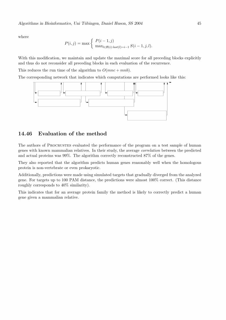
Algorithms in Bioinformatics, Uni Tubingen, Daniel Huson, SS 2004 45
where
P (i, j) = max
P (i− 1, j)maxl∈B(i):last(l)=i−1 S(i− 1, j, l).
With this modification, we maintain and update the maximal score for all preceding blocks explicitlyand thus do not reconsider all preceding blocks in each evaluation of the recurrence.
This reduces the run time of the algorithm to O(mnc+mnb).
The corresponding network that indicates which computations are performed looks like this:
14.46 Evaluation of the method
The authors of Procrustes evaluated the performance of the program on a test sample of humangenes with known mammalian relatives. In their study, the average correlation between the predictedand actual proteins was 99%. The algorithm correctly reconstructed 87% of the genes.
They also reported that the algorithm predicts human genes reasonably well when the homologousprotein is non-vertebrate or even prokaryotic.
Additionally, predictions were made using simulated targets that gradually diverged from the analyzedgene. For targets up to 100 PAM distance, the predictions were almost 100% correct. (This distanceroughly corresponds to 40% similarity).
This indicates that for an average protein family the method is likely to correctly predict a humangene given a mammalian relative.

Algorithms in Bioinformatics, Uni Tubingen, Daniel Huson, SS 2004 41
15 Suffix trees
This lecture is based on the following sources, which are all recommended reading:
• Dan Gusfield, Algorithms on strings, trees and sequences, Cambridge, 1997.
• R. Giegerich, S. Kurtz und J. Stoye. Efficient Implementation of Lazy Suffix Trees, WAE’99,LNCS 1668, pp. 30-42, 1999
• S. Kurtz, Foundations of sequence analysis, Bielefeld (2001).
History:Weiner 1973: linear-time algorithmMcCreight 1976: reduced spaceUkkonen 1995: new algorithm, easier to describe
15.1 Importance of sequence comparison
The first fact of biological sequence analysis: In biomolecular sequences (DNA, RNA, or amino acidsequences), high sequence similarity usually implies significant functional or structural similarity.
“Duplication with modification”: The vast majority of extant proteins are the result of a continuous
series of genetic duplications and subsequent modifications. As a result, redundancy is a built-in characteristic
of protein sequences, and we should not be surprised that so many new sequences resemble already known
sequences. . . . all of biology is based on enormous redundancy. . .
We didn’t know it at the time, but we found everything in life is so similar, that the same genes thatwork in flies are the ones that work in humans. (Eric Wieschaus, co-winner of the 1995 Nobel prize in medicine for work on the
genetics of Drosophia development.)
Dan Gusfield, 1997, 212 ff
15.2 Searching for short queries in a long text
Problem Given a long text t and many short queries q1, . . . , qk. For each query sequenceqi, find all its occurrences in t.
We would like to have a data-structure that allows us to solve this problem efficiently.
Example: The text t is a genomic sequence and the queries are short signals such as transcriptionfactor binding sites, splice sites etc.
Important applications are in the comparison of genomes (in programs such as MUMmer that computesmaximum unique matches) and in the analysis of repeats.

42 Algorithms in Bioinformatics, Uni Tubingen, Daniel Huson, SS 2004
15.3 Basic definitions
Let Σ denote an alphabet and Σ∗ the set of strings over Σ. Let ǫ denote the empty string andΣ+ = Σ∗ \ ǫ.Let t = t1t2 . . . tn be the text and $ ∈ Σ∗ \ t.For i ∈ 1, 2, . . . , n + 1, let si = ti . . . tn$ denote the i-th suffix of t$.
In bioinformatics, the alphabet Σ is usually of size 4 or 20. In other applications, the alphabet can bemuch larger, for example, to detect common web-surfing patterns, Σ may be very large, e.g. consistingof the set of all links contained in a collection of web sites.
15.4 The role of suffixes
Consider the text abab$
It has the following suffixes:
abab$, bab$, ab$, b$, and $.
To determine whether a given query q is contained in the text, we check whether q is the prefix of oneof the suffixes.
E.g., the query ab is the prefix of both abab$ and ab$.
To speed up the search for all suffixes that have the query as a prefix, we use a tree structure to sharecommon prefixes between the suffixes.
15.5 Sharing prefixes
(a) The suffixes abab$ and ab$ both share the prefix ab.
(b) The suffixes bab$ and b$ both share the prefix b.
(c) The suffix $ doesn’t share a prefix.
ba
$a
b$
(a)
b
$$b
a
(b)
$
(c)

Algorithms in Bioinformatics, Uni Tubingen, Daniel Huson, SS 2004 43
15.6 First example
1 3 2 4 5
abab$
ab$
bab$
$b$
⇒
ba
b$
$$
ab
$$b
a
1 3 2 4
5
Suffix tree for abab$ is obtained by sharing prefixes where ever possible. The leaves are annotated bythe positions of the corresponding suffixes in the text.
15.7 Σ+-tree
A Σ+-tree T is a finite, directed tree with root root . Its edges are labeled with strings in Σ+, suchthat: For every letter a ∈ Σ and node u there exists at most one a-edge u
as→ w (for some string s andsome node w).
av
w
u
A leaf is a node with no children and an edge leading to a leaf is called a leaf edge. A node with atleast two children is called a branching node.
15.8 Naming nodes by strings
Let u be a node of T . We use the name s for u, if s is the concatenation of all labels of the edgesalong the path from the root of the tree to u.
For example u = pqr:
u
p
q
r
root
The root is called ǫ.
Definition: A string g is said to occur in T , if there exists a string h such that gh is a node in T .

44 Algorithms in Bioinformatics, Uni Tubingen, Daniel Huson, SS 2004
15.9 Suffix tree
Definition: A suffix tree ST (t) for t is a Σ+-tree with the following properties:
1. Every node is either a leaf or a branching node, and
2. a string s occurs in ST (t) ⇔ s is a substring of t.
There exists a one-to-one correspondence between the non-empty suffixes of t$ and the leaves of ST (t).
For every leaf sj we define l(sj) = j. Recursively, for every branching node u we define:
l(u) = j | u v→ uv is an edge of ST (t), j ∈ l(uv).
In other words,
l(u) =⋃
v is child of u
l(v).
We call l(u) the leaf set of u.
15.10 Example
Text: xabxac
a
c$
bxac$
ac$
xb c
$c$
b xa c$
ax$
15.11 Ukkonen’s online construction
We will now discuss an algorithm that constructs ST (t) in linear time. It operates online and generates
ST (ǫ), ST (t1), ST (t1t2), . . . , ST (t1t2 . . . tn)
for all prefixes of t, without knowledge of the remaining part of the input string.
Induction: First, note that ST (ǫ) consists of a root node only. To completely define the algorithmwe must describe the induction step i→ i+ 1 or (i+ 1)-th phase:
ST (t1 . . . ti) to ST (t1 . . . titi+1), for any i < n.
More precisely, we will generate a series of so-called implicit suffix trees that can at any time be made“explicit” by processing a terminator character $.

Algorithms in Bioinformatics, Uni Tubingen, Daniel Huson, SS 2004 45
15.12 Implicit Suffix Tree
Every tree T computed by the induction step of Ukkonen’s algorithm is an implicit suffix tree in thefollowing sense:
Definition. An implicit suffix tree for string t is a tree obtained from the suffix tree for t$ by removingevery copy of the terminal symbol $ from the edge labels of the tree, then removing any edge that hasno label, and then removing any node that does not have at least two children.
Note that we will be able to obtain the latter from the former straight-forwardly in linear time, simplyby processing an additional terminator symbol $.
15.13 Updating the tree
Assume that T is an implicit suffix tree for t1 . . . ti. This means that any word w is contained in T ifand only if it is contained in t1 . . . ti.
Given the implicit suffix tree T = ST (t1 . . . ti), which modifications must we make to it to obtain anew tree T ′ = ST (t1 . . . titi+1) that represents all substrings of t1 . . . ti+1?
In the following we will use a := ti+1 to indicate the new letter currently being added to the text.
Let us consider each suffix wti+1 of t1 . . . ti+1 in turn. Note:
1. If wti+1 was already a substring of t1 . . . ti, then no modification to T is necessary to accommodatethis string.
2. If w is a leaf in T , then w occurs precisely once in t1 . . . ti and wti+1 also occurs precisely oncein the extended text t1 . . . titi+1. In this case, we can simply extend the label of the edge leadingto the leaf w by the letter ti+1.
3. Otherwise, w occurs at least twice in t1 . . . ti and wti+1 does not occur in t1 . . . ti. In this case,we call wti+1 a relevant suffix and the insertion of wti+1 is a more complex operation, which wewill describe in detail below.
15.14 Processing the suffixes
In the (i + 1)-th phase, the algorithm considers all extensions of suffixes w in order of decreasinglength: t1 . . . ti, t2 . . . ti etc.

46 Algorithms in Bioinformatics, Uni Tubingen, Daniel Huson, SS 2004
Note that the list of extensions can be partitioned as follows:
(A)
w1a = t1 . . . ti+1
. . .wpa = tp . . . ti+1
wj occurs precisely once in t1 . . . ti,
(B)wp+1a = tp+1 . . . ti+1
. . .wqa = tq . . . ti+1
wj is repeated in t1 . . . ti, butwja is not contained in t1 . . . ti,
(C)wq+1a = tq+1 . . . ti+1
. . .ǫa = ti+1
wja is contained in t1 . . . ti.
Each of these three sub-lists of prefixes is treated differently:
(A) To process suffixes w1a, . . . , wpa, simply extend all leaf edge labels by the new character a.
(B) To process all relevant suffixes wp+1a, . . . , wqa, insert each suffix into the tree T using theprocedure insert defined below.
(C) No processing of the suffixes wq+1 . . . ǫa is necessary as they are already contained in the tree.
15.15 Inserting a relevant suffix
To insert a relevant suffix wa into T , we must navigate into the tree matching as many letters of wato letters in edge-labels as possible. There are then two cases:
• If we finish matching letters inside an edge labeled uv, then we insert a new leaf edges as follows:
wti+1
w
wd
c+1...
u
v
u
v
• If we finish matching letters at a node uv, then we insert a new leaf edge under uv as follows:
wti+1
uv
u u
uvw
wd
c+1...
v v
15.16 Linear time construction
A O(n) runtime can be achieved by showing:

Algorithms in Bioinformatics, Uni Tubingen, Daniel Huson, SS 2004 47
1. how to extend all suffixes w1a, . . . , wpa in one step per phase,
2. that only ≤ n relevant suffixes occur throughout the whole run,
3. how to insert a relevant suffix in constant time, and
4. how to determine which suffixes are relevant in constant time.
Lemma: In each phase we can extend all suffixes w1a, . . . , wpa in one step.
This is because the label of any leaf edge ends at the end of the current text. Hence, we simplymaintain a global variable that contains the current text length and let this specify the end of all leaflabels.
Also, note that the topology of the tree is only changed when we process a relevant suffix and thisstep only modifies edges or internal nodes, but not leaves, hence: once a leaf, always a leaf.
Lemma: At most n relevant suffixes occur.
Proof: Let α(t1 . . . ti) denote the longest nested suffix in t1 . . . ti, i.e. the longest suffix that occursmore than once as a substring of t1 . . . ti. Then the total number of relevant suffixes that can occur is
R =
n−1∑
i=1
(qi − pi) =
n−1∑
i=1
(|α(t1 . . . ti)a| − |α(t1 . . . ti+1)|)
=n−1∑
i=1
(|α(t1 . . . ti)|+ 1− |α(t1 . . . ti+1)|)
= n− 1 + |α(t1)| − |α(t1 . . . tn)| ≤ n,where pi and qi denote the values of p and q in the i-th phase.
15.17 Tracking the location of a suffix
To be able to perform steps (3) and (4) in constant time, we define the concept of the location of asuffix in the tree T and keep track of our current location in the tree.
For a string s contained in T , define loc(s) as follows:
• if s is a branching node, then set loc(s) := s,
• if s is a leaf, then there is a leaf edge uv−→ s in T and we set loc(s) := (u, v, ǫ, s),
• otherwise, there is an edge uvw−→ uvw such that s = uv, v 6= ǫ, w 6= ǫ and we set loc(s) :=
(u, v,w, uvw).
Additionally, we will introduce so-called suffix links that will help us to navigate through the tree aswe move down the list of suffixes for a given phase.

48 Algorithms in Bioinformatics, Uni Tubingen, Daniel Huson, SS 2004
15.18 Operations on locations
We define the following three operations on locations:
(1) Given the location loc(w) of a suffix w of t1 . . . ti in T and a new letter a, determine whether waoccurs in T , that is, define occurs(loc(w), a) := true ⇔ wa occurs in T . This operation can beimplemented in constant time.
This tells use when we have seen the last relevant suffix in the current phase.
(2) Given the location loc(s) of a string s and a string w such that sw occurs in T . The operationgetloc(loc(s), w) := loc(sw) returns the location of sw in T in O(|w|) time, simply by followingcharacters of w in T .
This will be used to update so-called “suffix links”, as described defined below.
(3) Given a suffix s of t1 . . . ti and loc(s), if sa is relevant, then we insert it into the tree as follows:
– if loc(s) = s, then s is a branching node and we add a leaf edge sa−→ sa, and
– otherwise, loc(s) = (u, v,w, uvw) and we update the tree by splitting the edge uvw−→ uvw
into uv−→ s
w−→ uvw and adding a new leaf edge sa−→ sa.
This is the most important operation that inserts a relevant suffix sa into the tree T .
15.19 Suffix links
To be able to process the list of relevant suffixes in the i-th phase quickly enough, we need to be ableto move from loc(bw) to loc(w) in constant time.
To facilitate this, we maintain for each branching node, say bw, an auxiliary edge called a suffix linkthat points to the branching node w, if it exists, or to the root, else.
In the operation insert(loc(s), a) described above, we update the suffix links as follows:
• If loc(s) = s, then no new internal node is generated and we do nothing.
• Otherwise, assume that loc(s) = (u, v,w, uvw) and s is obtained as described above. Then thetarget of the suffix link from s is given by the following location:
linkloc(s) :=
loc(v2 . . . vk) if u = root , andgetloc(linkloc(u), v) else,
where v = v1 . . . vk.
15.20 Example
A suffix tree with a suffix links (dotted arcs):

Algorithms in Bioinformatics, Uni Tubingen, Daniel Huson, SS 2004 49
a
acbaca
bca
bc
cb
c
a
a
Locations: locT (ǫ) = root
locT (a) = (root , a, bca, abca)
locT (abca) = (root , abca, ǫ, abca)
locT (bc) = (root , bc, a, bca)locT (c) = c
locT (cab) = (c, ab, ca, cabca)
15.21 Ukkonen’s algorithm
AlgorithmInput: text t1 . . . tnOutput: chain of implicit suffix trees ST (t1), . . . , ST (t1 . . . tn)Initialization: Generate a single node ǫ and set L = ǫ.for i = 1 to n do // phase i generates ST (t1 . . . ti)
while occurs(L, ti) = false do // for all relevant suffixesif L is not a leaf then // i.e., not of the form (u, v, ǫ, uv)
insert(L, ti) // insert the suffixSet L := linkloc(L) // move to next suffix
Set L := getloc(L, ti) // prepare for next phaseend
This generates an implicit suffix tree ST (t1 . . . ti) for each i. (Recall that all leaf labels are implicitlyextended as we assume that they extend to the last processed position in the text.) To obtain a fullsuffix tree for the text t1 . . . ti, simply run the main loop one more time using a character $ that doesnot occur in the text.
Theorem This algorithm builds the suffix tree ST (t1 . . . tn) by inserting ≤ n relevant suffixes, eachin constant time, thus achieving a linear run time.
15.22 Example
Consider the text pucupcupu. Each column contains all suffixes of a prefix of the string:

50 Algorithms in Bioinformatics, Uni Tubingen, Daniel Huson, SS 2004
i : 0 1 2 3 4 5 6 7 8 9ǫ ↓p pu puc pucu pucup pucupc pucupcu pucupcup pucupcupu
ǫ ↓u uc ucu ucup ucupc ucupcu ucupcup ucupcupuǫ ↓c cu cup cupc cupcu cupcup cupcupu
ǫ u ↓up upc upcu upcup upcupuǫ p ↓pc pcu pcup pcupu
ǫ c cu cup ↓cupuǫ u up ↓upu
ǫ p pu
ǫ uǫ
The relevant suffixes sa are marked by ↓. Suffixes actually looked at by the algorithm are underlined.The suffixes that causes the while loop to break are underlined twice.
15.23 The WOTD Algorithm
Ukkonen’s algorithm can build the suffix tree in linear time. Although this is a nice algorithm, it hastwo draw-backs:
First, it does not have good memory locality, which means that there is little correlation between howclose two pieces of data are in the tree, and how close they are in physical memory. Hence, an averagequery will produce many cache misses and can lead to poor performance in practice.
Second, if we only have a few queries to pose, then it may be wasteful to compute the whole suffixtree.
The “write only, top down” algorithm due to R. Giegerich, S. Kurtz and J. Stoye (1999) has goodmemory locality and can also be used for a lazy construction of the suffix tree, building only as muchof the tree as is necessary to satisfy a given query.
Although it requires O(n log n) average run-time, in practice it is often competitive.
15.24 Idea: Compute tree recursively
Note that the subtree below a branching node u is determined by the set of all suffixes of t$ that startwith the prefix u:
US1
US2USk
U
S1 S2
U
Sk
...
...

Algorithms in Bioinformatics, Uni Tubingen, Daniel Huson, SS 2004 51
So, if we know the set of remaining suffixes
R(u) := s | us is a suffix of t$,
then we can evaluate the node u, i.e. construct the subtree below u.
15.25 The main evaluation step
An unevaluated node is evaluated as follows: We partition the set R(u) into groups by the first letterof the strings, i.e. for every letter c ∈ Σ, we define the c-group as:
Rc(u) := cw ∈ Σ∗ | cw ∈ R(u).
Consider Rc(u) for c ∈ Σ. If Rc(u) 6= ∅, then there are two possible cases:
1. If Rc(u) contains precisely one string w, then we construct a new leaf edge starting at u andlabel it with w.
2. Otherwise, the set Rc(u) contains at least two different strings and let p denote their longestcommon prefix (lcp). We create a new c-edge with label p whose source node is u. The newunevaluated node up and set R(up) = w | pw ∈ Rc(u) will be (recursively) processed later.
15.26 Evaluating the root
This wotd-algorithm (write-only, top-down) starts by evaluating the root node, with R(root) equal tothe set of all suffixes of t$. All nodes of ST (t) are then recursively constructed using the appropriatesets of remaining suffixes.
15.27 Example
Text: abab$
The algorithm proceeds as follows: We first evaluate the root node root using R(root) =abab$, bab$, ab$, b$. There are three groups of suffixes:
Ra(root) = abab$, ab$, Rb(root) = bab$, b$ and R$ = $.
The letter $ gives rise to a leaf edge with label $. The letter a gives rise to an internal edge with labelab, because ab = lcp(Ra(root)). Similarly, for b we obtain an internal edge with label b.
For the node ab we have R(ab) = ab$, $ and thus Ra(ab) = ab$ and R$(ab) = $. Because bothlatter sets have cardinality one, we obtain two new leaf edges with labels ab$ and $, respectively.
Similarly, we obtain two new leaf edges with labels ab$ and $ for the node b.
Text: abab$

52 Algorithms in Bioinformatics, Uni Tubingen, Daniel Huson, SS 2004
abab$bab$ab$b$$
R(root):
⇒R(ab): R(b):
ba
b$
ab$$
ab$$
⇒
ba
b$
$$
ab
$$b
a
15.28 Properties of the wotd-algorithm
Complexity: Space requirement? Worst case time complexity? (Exercises!)
The expected running time is O(n logk n) and experimental studies indicate that the algorithm oftenperforms in linear time for moderate sized strings.
Good memory locality.
Algorithm can be parallelized.
15.29 Suffix tree data-structure
An implementation of a suffix tree must represent its nodes, edges and edge labels. To be able todescribe the implementation, we define a total ordering on the set of children of a branching node:
Let u and v be two different children of the same node in ST (t). We write
u ≺ v iff min l(u) < min l(v),
in other words, iff the first occurrence min l(u) of u in t$ comes before the first occurrence min l(v) ofv in t$.
u v u
min l(u) min l(v)
vt

Algorithms in Bioinformatics, Uni Tubingen, Daniel Huson, SS 2004 53
15.30 Representing edge labels efficiently
Remark 1 Because an edge label s is a substring of the text t$, we can represent it by a pair ofpointers (i, j) into t′ = t$ such that s = t′i, t
′i+1, . . . , t
′j .
However, note that we have j = n + 1 for any leaf edge and so in this case the right pointer isredundant. Hence:
Remark 2 A leaf edge requires only one pointer.
The following is not so easy to see:
Remark 3 An internal edge requires only one pointer.
This is made possible by defining a left pointer on the set of nodes (not edges) in such a way thatthese can be used to reconstruct the original left and right pointers of each edge, as follows:
Consider an edge uv→ uv. Define the left pointer of uv as the position p of the first occurrence of uv
in t$ plus the length of u:lp(uv) = min l(uv) + |u|.
This gives the start position i of a copy of v in t$.
To get the end position of v, consider the ≺-smallest child uvw of uv. We have min l(uv) = min l(uvw),i.e. the corresponding suffix starts at the same position p. By definition, we have lp(uvw) =min l(uvw) + |uv| and the end position of v equals lp(uvw)− 1.
t vu w
lp(uvw)lp(uv)
min l(uv)=min l(uvw)i r
15.31 The main data table
For each node u, we store a reference firstchild(u) to its smallest child.
We store the values of lp and firstchild together in a single (integer) table T . We store the values of allchildren of a given node u consecutively, ordered w.r.t. ≺. (We will indicate the last child of u by setting
its lastchild -bit.)
So, only the edge from a given node u to its first child is represented explicitly. Edges from u to itsother children are given implicitly and are found be scanning consecutive positions in T that followthe position of the smallest child.
We reference the node u using the index of the position in T that contains the value lp(u).
15.32 Example
The table T for ST (abab). All indices start at 1. The first value in T for a branching node u is lp(u),the second value is firstchild(u):

54 Algorithms in Bioinformatics, Uni Tubingen, Daniel Huson, SS 2004
node ab b $ abab$ ab$ bab$ b$︷︸︸︷ ︷︸︸︷ ︷︸︸︷ ︷︸︸︷ ︷︸︸︷ ︷︸︸︷ ︷︸︸︷
T 1 6 2 8 5 3 5 3 5
Index 1 2 3 4 5 6 7 8 9
Bits ∗ † ∗ ∗ † ∗ ∗ †To be able to decode this representation of the suffix tree, we need two extra bits: A leaf-bit (∗)indicates that the given position in T corresponds to a leaf node and a lastchild-bit (†) indicates thatthe node at this position does not have a larger brother w.r.t. ≺.
15.33 Storing an unevaluated node
We consider the wotd-algorithm as a process that evaluates the nodes of a suffix tree. It starts at theroot and then evaluates all nodes recursively.
First we discuss how to store an unevaluated node u.
To be able to evaluate u, we (only) need to know the set of remaining suffixes R(u). To make theseavailable, we define a global array called suffixes that contains pointers to suffixes in t$ and use itas follows: For every unevaluated node u, the suffixes array contains an interval of pointers to startpositions in t$ that correspond precisely to the suffixes contained in R(u), in increasing order.
We can now represent R(u) in T using two numbers, left(u) and right(u), that define an interval ofentries in the suffixes array.
As a branching node, u will occupy two positions in T , one for lp(u) and followed by firstchild(u).Until u is actually evaluated, we will use these two positions to store left(u) and right(u). We use athird bit called the unevaluated -bit to distinguish between unevaluated and evaluated nodes.
15.34 Evaluating a node u
First note that the left pointer lp(u) of the node u is given by the left-most entry of suffixes over theinterval [left(u), right (u)].
Determine the length of the longest common prefix lcp of entries in suffixes over [left(u), right(u)] andadd it to all these entries.
The lcp is computed by stepping through a simple loop j = 1, 2 . . . and checking the equality of allletters tsuffixes[i]+j for all start positions i in [left(u), right(u)]. As soon as a difference is detected, theloop is aborted and j is the length of the lcp.
Sort and count all entries of suffixes in the interval [left(u), right(u)], by the first letter c of the suffixesas the sort key. (Do this stably, i.e. don’t change the order of suffixes that start with the same letter.)
Each letter c that has count > 0 will give rise to a new node v below u and the suffixes in the c-groupRc(u) determine the tree below v.
For each non-empty c-group of u, we store one child in the table T , as follows:
Leaf case: A c-group containing only one string gives rise to a leaf node v and we write the numberlp(v) in the first available position of T . This number lp(v) is obtained as the single entry of suffixes

Algorithms in Bioinformatics, Uni Tubingen, Daniel Huson, SS 2004 55
that corresponds to the c-group.
Internal node case: A c-group containing more than one string gives rise to branching node v andwe store left(v) and right(v) in the first two available positions of T . The values of left and right arecomputed during the sort and count step.
15.35 Lazy vs. complete evaluation
To build the complete suffix tree, we proceed breath-first, from left to right.
In a lazy approach, we only evaluate those nodes that are necessary to answer a query (and have notyet been evaluated).
15.36 Example
Input: Text: a b a b $1 2 3 4 5
Initial.: suffixes : 1 2 3 4 5 T :
Evaluate(root):Sort and count: Ra(root ) = 1, 3, lcp = ab
Rb(root ) = 2, 4, lcp = bR$(root ) = 5
The suffixes are ordered, left and right are entered in the table and the three bits (u, ∗, †:unevaluated , leaf , lastchild) are set:
suffixes : 1 3 2 4 5 T : 1 2 3 4 5u u ∗†
(Text : a b a b $
1 2 3 4 5
)
Evaluate(1):Note lp(1) = suffixes [T [1]] = suffixes [1] = 1 and firstchild(1) = 6, thus:
T : 1 6 3 4 5u ∗†
Determine lcp of entries suffixes [1 . . . 2] and add it to them:suffixes : 3 5 2 4 5
Determine c-groups and then add appropriate nodes:Ra(1) = 3R$(1) = 5T : 1 6 3 4 5 3 5
(u) u ∗† ∗ ∗†(
Text : a b a b $1 2 3 4 5
)

56 Algorithms in Bioinformatics, Uni Tubingen, Daniel Huson, SS 2004
Evaluate(3):Note lp(3) = suffixes [T [3]] = suffixes [3] = 2 and firstchild(3) = 8, thus:
T : 1 6 2 8 5 3 5u ∗† ∗ ∗†
Determine lcp of entries suffixes [3 . . . 4] and add it to them:suffixes : 3 5 3 5 5
Determine c-groups and then add appropriate nodes:Ra(3) = 3R$(3) = 5
T : 1 6 2 8 5 3 5 3 5(u) ∗† ∗ ∗† ∗ ∗†
Done!
15.37 Finding occurrences in a WOTD tree
Suppose we are given a text text and have computed the WOTD tree T . How do we determine alloccurrences of a given query string q?
This is done by navigating into the tree and matching the letters of the query with the letters of theedge labels until we have used-up all the letters of the query. Once we have established that the queryis contained in the tree, we visit all nodes below the location at which the query was fullfilled andreport one occurrence for each leaf.
Recall that the position of an occurrence is not stored in the tree, however, it can be obtained bykeeping track of the depth of nodes which is the the sum of lengths of all edge labels along the pathfrom the root to the node.
The following algorithm is initially called with t = 1, the first cell in T :
Algorithm Find-WOTDInput: A query stringOutput: All occurrences of queryrepeat
label := getEdgeLabel(t)newDepth := depth+ |edgeLabel|compare query and labelif query is prefix of label then // query found
if t is leaf thenreturn the singleton list |text| − newDepth
else return collectAllHits(T [t+ 1], newDepth)else if label is proper prefix of query then // move to child
t := T [t+ 1], depth := newDepth,query := query[|label|+ 1, |query|]
else if query[0] = label[0] then return empty-list // not in treeelse // try next child, if available
if t is last child then return empty-list

Algorithms in Bioinformatics, Uni Tubingen, Daniel Huson, SS 2004 57
if t is leaf then t := t+ 1 else t := t+ 2 // move to siblingend
Sub-Routine collectAllHits (t, depth)Input: A parent node t and it’s depth below the rootReturns: List hits of all positions corresponding to leaves below trepeat
newDepth = depth+ |getEdgeLabel(t)|if t is a leaf then
Append (|text| − newDepth) to hitsif t is last child, returnt := t+ 1
elsecall collectAllHits(T [t+ 1], newDepth)if t is last child, returnt := t+ 2
end
Sub-Routine getEdgeLabel (t)Input: A node tReturns: The corresponding edge labelbeginSet p1 = T [t]if t is a leaf node then
Set p2 = |text|else
Set p2 = T [T [t+ 1]]− 1return text[p1, p2]end
15.38 Applications of suffix trees
1. Searching for exact patterns
2. Minimal unique substrings
3. Maximal unique matches
4. Maximal repeats
5. Approximate repeats
Additional literature:
Stefan Kurtz, Enno Ohlebusch, Chris Schleiermacher, Jens Stoye and Robert Giegerich, Computation and
visualization of degenerate repeats in complete genomes, ISMB 2000, p. 228-238, 2000.

58 Algorithms in Bioinformatics, Uni Tubingen, Daniel Huson, SS 2004
Stefan Kurtz and Chris Schleiermacher, REPuter: fast computation of maximal repeats in complete genomes,
Bioinformatics, 15(5):426-427 (1999)
15.39 Searching for exact patterns
To determine whether a string q occurs in a string t, follow the path from the root of suffix tree ST (t)as directed by the characters of q. If at some point you cannot proceed, then q does not occur in t,otherwise it does.
Text abab$.
ba
b$
$$
ab
$$b
a
1 3 2 4
5
The query abb is not contained in abab: Following ab we arrive at the node ab, however there is no b-edge leaving
from there. The query baa is not contained in abab: Follow the b edge to b and then continue along the leaf
edge whose label starts with a. The next letter of the label is b and doesn’t match the next letter of the query
string.
Clearly, the algorithm that matches a query q against the text t runs in O(|q|) time.
15.40 Finding all occurrences
To find all positions where the query q is contained in t, annotate each leaf si of the suffix tree withthe position i at which the suffix i starts in t.
Then, after matching q to a path in the tree, visit all nodes below the path and return the annotatedvalues.
This works because any occurrence of q in t is the prefix of one of these suffixes.
The number of nodes below the path is at most twice the number of hits and thus finding and collectingall hits takes time O(|q|+ k), where k is the number of occurrences.
(Note that in the discussed lazy suffix tree implementation we do not use this leaf annotation but rather compute
the positions from the the lp values, to save space...)
15.41 Application: Maximal Unique Matches
Standard dynamic programming is too slow for aligning two large genomes. If the genomes are similar, then
one can expect to see long identical substrings which occur in both genomes. These maximum unique matches
(MUMs) are almost surely part of a good alignment of the two sequences and so the alignment problem can be
reduced to aligning the sequence in the gaps between the MUMs.
Given two sequences s and t, and a number l > 0. The maximal unique matches problem (MUM-problem) is to find all sequences u with:

Algorithms in Bioinformatics, Uni Tubingen, Daniel Huson, SS 2004 59
• |u| ≥ l,
• u occurs exactly once in s and once in t, and
• for any character a neither ua nor au occurs both in s and t.
In other words, a MUM is a sequence m that occurs precisely once in s and once in t, and is bothright maximal and left maximal with this property.
This problem can be solved in O(|s|+ |t|) time: To find all MUMs, generate the suffix tree T for s%t,where % is a “separator” with % /∈ s and % /∈ t. Any path in T from the root to some node u thathas precisely two children, one in s and one in t, corresponds to a right maximal unique match.
To determine whether u is left maximal, too, simply check whether both preceding letters in s and tdiffer.

60 Algorithms in Bioinformatics, Uni Tubingen, Daniel Huson, SS 2004
15.42 Example
15.43 Example

Algorithms in Bioinformatics, Uni Tubingen, Daniel Huson, SS 2004 61
15.44 Repeats in human
(Nature, vol. 409, pg. 880, 15. Feb 2000)
15.45 Definition of a maximal repeat
Given a sequence t = t1t2 . . . tn.
A substring t[i, j] := ti . . . tj is represented by the pair (i, j). A pair R = (l, r) of different substringsl = (i, j) and r = (i′, j′) of t is called a repeat, if i < i′ and ti . . . tj = ti′ . . . tj′. We call l and r theright and left instance of the repeat R, respectively.
t ... tjit ... ti’ j’
i j i’ j’
=t
A repeat R = ((i, j), (i′ , j′)) is called left maximal, if i = 1 or ti−1 6= ti′−1, and right maximal, if j′ = nor tj+1 6= tj′+1, and maximal, if both.
t ... tjit ... ti’ j’
i j i’ j’
=ta b c d
maximal ⇔ a 6= c and b 6= d
15.46 Example
The string1 2 3 4 5 6 7 8 9 10g a g c t c g a g c contains the following repeats of length ≥ 2:

62 Algorithms in Bioinformatics, Uni Tubingen, Daniel Huson, SS 2004
((1, 4), (7, 10)) gagc
((1, 3), (7, 9)) gag((2, 4), (8, 10)) agc((1, 2), (7, 8)) ga((2, 3), (8, 9)) ag((3, 4), (9, 10)) gc
15.47 An algorithm for computing all maximal repeats
We will discuss how to compute all maximal repeats. Let t be a string of length n and assume thatthe first and last letter of t both occur exactly once on t, e.g.:
1 2 3 4 5 6 7 8 9 10 11 12 13t = x g g c g c y g c g c c z
Let T be the suffix tree for t.
We can ignore all leaf edges from the root.
The algorithm proceeds in two phases:
In the first phase, every leaf node v of T is annotated by (a, i), where v = ti . . . tn is the suffix associatedwith v and a = ti−1 is the letter that occurs immediately before the suffix.
15.48 Example
Partial suffix tree for1 2 3 4 5 6 7 8 9 10 11 12 13
t = x g g c g c y g c g c c z :
c
ygcgccz
gczc
ygcgccz
ygcgccz
gcgcygcgccz
g
cz
gccz
ygcgcczcz
cz
With leaf annotations:

Algorithms in Bioinformatics, Uni Tubingen, Daniel Huson, SS 2004 63
c
ygcgccz
gczc
ygcgccz
ygcgccz
gcgcygcgccz
g
cz
gccz
ygcgcczcz
c 10
c 12 g 11g 9 g 4
g 6
x 2c 5
y 8 g 3
cz
15.49 Second phase of the algorithm
For every leaf node v set:
A(v, c) =
i, if c = ti−1, and∅, else,
where i is the start position of the corresponding suffix v.
In the second phase of the algorithm, we extend this annotation to all branching nodes bottom-up:
Let w be a branching node with children v1 . . . vh and assume we have computed A(vj , c) for allj ∈ 1, . . . , h and all c ∈ Σ.
For each letter c ∈ Σ set:
A(w, c) :=
h⋃
j=1
A(vj , c).
Note that this is a disjoint union and A(w, c) is the set of all start positions of w in t for whichti−1 = c.
15.50 Example
1 2 3 4 5 6 7 8 9 10 11 12 13t = x g g c g c y g c g c c z
g 3c 5,10x 2y 8
c 5,10y 8
g 3
g 3y 8
c
ygcgccz
ygcgccz
gcgcygcgccz
g
gc
c 10
x 2c 5
y 8 g 3
cz
cz
((8,9),(10,11))((3,4),(10,11)((5,6),(8,9))((3,4),(5,6))
((3,6),(8,11))

64 Algorithms in Bioinformatics, Uni Tubingen, Daniel Huson, SS 2004
Annotation of branching nodes and output repeats of length ≥ 2
15.51 Reporting all maximal repeats
In a bottom-up traversal, for each branching node w we first determine A(w, c) for all c ∈ Σ and thenreport all maximal repeats of the word w:
Let q be the current depth, i.e. number of characters from the root node, i.e. the length of w.
If depth ≥ l do:
for each pair of children vf and vg of w with vf ≺ vg:for each letter c ∈ Σ with A(vf , c) 6= ∅:
for each i ∈ A(vf , c):for each letter d ∈ Σ with d 6= c and A(vg, d) 6= ∅:
for each j ∈ A(vg, d):Print ((i, i + q − 1), (j, j + q − 1))
end
15.52 Maximality of output
Lemma The algorithm prints precisely the set of all maximal repeats in t of length ≥ l.Proof
1. Each printed pair R is a repeat, as the word w is the common prefix of two or more differentsuffixes.
2. Each repeat R is left-maximal, as c 6= d.
3. Each repeat R is right-maximal, as vf 6= vg, and by definition of a suffix tree, the labels of theedges leading to these two children begin with distinct letters.
4. No maximal repeat is reported twice, as vf ≺ vg and all unions are disjoint.
15.53 Performance analysis
Lemma Computation of all maximal repeats of length ≥ l can be done in O(n + z) time and O(n)space, where z is the number of maximal repeats.
Proof The suffix tree can be built in O(n) time and space. We can annotate the tree in O(n) time andspace, if we use the fact that we only need to keep the annotation of a node until its father has beenfully processed. (Also, we maintain the sets as linked links and then each disjoint-union operation canbe done in constant time.)
In the nested loop we enumerate in total all z maximal repeats in O(z) steps.
Hence, the algorithm is both time and space optimal.

Algorithms in Bioinformatics, Uni Tubingen, Daniel Huson, SS 2004 65
15.54 Significance of repeats
How significant is a detected maximal repeat? In a long random text we will expect to find manyshort repeats purely by chance.
The E-value associated with a maximum repeat R in t is the expected number of repeats of the samelength or longer that are found in a random sequence of length |t|.To compute this in the case of DNA, consider a simple Bernoulli model where each base α ∈A,C,G, T has the same fixed probability of occurrence: pα = p = 1
4 .
Note that the number of maximal exact repeats of length ≥ l equals the number of (only) left-maximalrepeats of length exactly l.
Ignoring boundary effects:
E[# of maximal exact repeats of length ≥ l]
= E[# of left-maximal exact repeats of length l]
=∑
1≤i1<i2≤n
Pr(t[i1, i1 + l − 1] = t[i2, i2 + l − 1], ti1−1 6= ti2−1)
=∑
1≤i1<i2≤n
pl(1− p)
=1
2n(n− 1)pl(1− p)
With boundary effects: = 12(n− l + 1)(n − l)pl(1− p) + (n− l)pl+1.
(Note that this is only an estimation, as the effect of overlapping of instances of the repeat is ignored.)
15.55 Palindromic repeats
Let t be a DNA sequence. We call ((i, j), (i′ , j′)) a palindromic repeat, if ti . . . tj = ti′ . . . tj′, where wdenotes the reverse complement of a DNA string w.
All maximal palindromic repeats can be found using a modification of the described algorithm formaximal repeats, based on the suffix tree for xtytz, where x, y, z are three characters that do notappear in t or t.
15.56 Degenerate repeats
Let u and w be two strings of the same length. The Hamming distance dH(u,w) between u and w isthe number of positions i such that ui 6= wi.
In the following, we assume that we are given a sequence t = t1 . . . tn, an error threshold k ≥ 0 and aminimum length l > 0.

66 Algorithms in Bioinformatics, Uni Tubingen, Daniel Huson, SS 2004
Definition A pair of equal-length substrings R = ((i1, j1), (i2, j2)) is called a k-mismatch repeat int, iff (i1, j1) 6= (i2, j2) and dH(t[i1, j1], t[i2, j2]) = k. The length of R is j1 − i1 + 1 = j2 − i2 + 1. Ak-mismatch repeat is maximal if it is not contained in any other k-mismatch repeat.
As with exact repeats, a k-mismatch repeat R = ((i1, j1), (i2, j2)) is maximal iff (i1 = 1 or i2 = 1 orti1−1 6= ti2−1) and (j1 = n or j2 = n or tj1+1 6= tj2+1)
15.57 The Mismatches Repeat Problem
The Mismatches Repeat Problem (MMR) is to enumerate all maximal k-mismatch repeats of length≥ l contained in t.
15.58 Example
Maximal k-mismatch repeats (k = 0, . . . , 4) for l = 5 in mississippi:
1 2 3 4 5 6 7 8 9 10 11text : m i s s i s s i p p i
k = 0 : nonek = 1 : s i s s i
m i s s ik = 2 : s i p p i
s i s s ik = 3 : s i p p i
m i s s ik = 4 : ???
15.59 The Seed Lemma
The following result is a key observation and is the basis of many seed-and-extend approaches tosequence comparison:
Lemma Every maximal k-mismatch repeat R of length l contains a maximal exact repeat of length≥ ⌊ l
k+1⌋, called a seed.
Proof Let R = ((i1, j1), (i2, j2)) be a k-mismatch repeat of length ≥ l. The k mismatches dividet[i1, j1] and t[i2, j2] into exact repeats w0, w1, . . . , wk. Now maxi∈[0,k] |wi| is minimal if the mismatchingcharacter pairs are equally distributed over R. Obviously, for such an equal distribution the length ofthe longest wi is ≥ ⌈ l−k
k+1⌉ = ⌊ lk+1⌋.
(A “•” indicates a mismatch and we have: l = 11, k = 3, ⌈ l−kk+1⌉ = ⌈ 11−3
3+1⌉ = ⌈ 8
4⌉ = 2 = ⌊ l
k+1⌋ = ⌊ 11
3+1⌋)

Algorithms in Bioinformatics, Uni Tubingen, Daniel Huson, SS 2004 67
15.60 An algorithm for the MMR problem
Suppose we are given a text t of length n. To find all maximal k-mismatch repeats in t of length ≥ l,do the following:
1. Build the suffix tree T for t and use it to detect all seeds, i.e., all exact maximal repeats of length≥ ⌊ l
k+1⌋.
2. For each seed s = ((i1, j1), (i2, j2)) do the following:
(a) For q = 0, 1, . . . k, compute:left(q) := maxp | dH(t[i1−p, i1], t[i2−p, i2]) = q, i.e. the length of the maximal extensionof the seed to the left with precisely q mismatches.
(b) For q = 0, 1, . . . k, compute:right(q) := maxp | dH(t[j1, j1 + p], t[j2, j2 + p]) = q, i.e. the length of the maximalextension of the seed to the right with precisely q mismatches.
(c) For q = 0, 1, . . . k:If (j1 − i1 + 1 + left(q) + right(k − q)) ≥ l, then print ((i1 − left(q), j1 + right(k − q)), (i2 −left(q), j2 + right(k − q))).
15.61 Correctness of the algorithm
The correctness of the algorithm follows from the Seed Lemma: every maximal k-mismatch repeat oflength ≥ l contains an exact repeat of length ≥ ⌊ l
k+1⌋ and can be obtained from the seed by extendingthe seed match with q mismatches to the left and with k− q mismatches to the right, for some q ≤ k.Note that the same maximal k-mismatch repeat can be obtained via more than one seed. To avoidthis, when computing left for a given seed, we stop the computation of the table left, if we observe asecond seed to the left of the original seed. This ensures that we only output those maximal k-mismatchrepeats for which the given seed is leftmost.
15.62 Efficient solution of MMR problem
Lemma The mismatch repeats problem MMR can be solved in O(n+ kq) time, where n is the lengthof the text, k is the number of mismatches permitted and q is the number of different seeds.
We can find all seeds in O(n + q) time. Thus the result follows, if we can compute the k-mismatchextension of any seed in k steps.
The latter can indeed be achieved, if we can determine the maximal common extension of two matchesin constant time. This is indeed possible, due to the following amazing result on rooted trees:
15.63 The lowest common ancestor problem
Let T be a rooted tree. A node u is called an ancestor of a node v iff u lies on the unique path fromroot to v. The lowest common ancestor (lca) of two nodes i and j is the last node that is both on the

68 Algorithms in Bioinformatics, Uni Tubingen, Daniel Huson, SS 2004
path from root to i and on the path from root to j.
Theorem Let T be a rooted tree. After a linear amount of preprocessing, we can determine the lowestcommon ancestor of any two nodes x and y in constant time.
(This is due to Harel and Tarjan (1984) and later simplified by Schieber and Vishkin (1988), see Chapter 8 of
Dan Gusfield’s book for details.)
15.64 Determining whether one node is an ancestor of another
In the the lowest common ancestor problem, there is a particularly simple case, namely when onenode, i say, is an ancestor of the other, j say.
Consider two nodes i and j in a rooted tree T . How to determine whether i is an ancestor of j inconstant time, after a linear amount of preprocessing?
Preprocess the tree as follows: number all nodes in a depth-first traverse and let l(i) denote the depth-first number of i. Let s(i) denote the number of nodes (including i) contained in the subtree rootedat i, obtained as the count of depth-first numbers used while processing i.
Lemma Node i is an ancestor of node j if and only if l(i) ≤ l(j) and l(j) ≤ l(i) + s(i).
15.65 Complete binary trees
How to compute the least common ancestor lca(i, j) of two nodes i and j in the case that lca(i, j) /∈i, j? We will discuss this for the simple case of a complete binary tree. (See Gusfield 1997 for thegeneral case.)
In the following, suppose that T is a rooted complete binary tree with p leaves, and n = 2p− 1 nodesin total, such that every internal node has precisely two children and the number of edges on the pathfrom the node to any leaf is d = log2 p.
15.66 Computational Model
Any run-time complexity analysis is based on a computational model. Given an input of size n, weusually assume the unit cost RAM model, in which:
• any number of size O(log n) bits can be written, read or used as an address in constant time,and
• any two O(log n)-bit numbers can be added, subtracted, multiplied or divided in constant time.
In the following we also explicitly assume that bit operations such as exclusive-or (XOR), left- orright-shift and detecting the first non-zero bit can be performed in constant time on numbers of sizeO(log n).

Algorithms in Bioinformatics, Uni Tubingen, Daniel Huson, SS 2004 69
15.67 In-order node numbering
Let us assume that the nodes of T have been numbered using an in-order traverse. We will view thesein-order numbers as bit-strings of length d+ 1, e.g.:
0001 0011 0101 0111 1001 1011 1101 1111
1110101001100010
0100 1100
1000
Alternatively, we may consider assigning to each node v a d+ 1-bit number called the path number ofv, defined as follows.
Counting from the left-most bit, the kth bit in the path number of v corresponds to the kth edge inthe path from the root to v: a 0 indicates that the path goes to a left child and a 1 indicates that thepath goes to a right child. The right-most 1 indicates the end-of-path (and not a choice of child).
For example, 0110 is the node obtained by choosing the left child of the root and then the right childof that node.
We have:
Lemma The in-order number of a node equals its path number.
15.68 Solving lca for a complete binary tree
Let T be a complete binary tree with an in-order numbering of nodes. How to compute lca(i, j) inconstant time, after a linear amount of preprocessing, when lca(i, j) /∈ i, j?Let xij = XOR(i, j) be the number obtained by computing the bitwise-exclusive-or of the two d+1-bitnumbers i and j.
Let k denote the position of the left-most 1 of xij . By definition of XOR, the first k − 1 bits of i andj are the same and thus the paths to i and j are the same for the first k − 1 edges, and then diverge(as we are assuming lca(i, j) /∈ i, j).Hence, the path-number for lca(i, j) consists of the first k − 1 bits of i, followed by a 1 (to indicateend-of-path), followed by d+ 1− k zeros.
Example:
i = 0 0 1 0
j = 0 1 1 1
XOR(i, j) = 0 1 0 1
→ k = 2result: 0 1 0 0
So, we can compute lca(i, j) in constant time using the following bit-operations:
• compute xij = XOR(i, j)

70 Algorithms in Bioinformatics, Uni Tubingen, Daniel Huson, SS 2004
• Determine the position k of the left-most 1 in xij
• Shift i to the right by d+ 1− k places
• Set the right-most bit of i to 1
• Shift i to the left by d+ 1− k places.

Algorithms in Bioinformatics, Uni Tubingen, Daniel Huson, SS 2004 65
16 Suffix arrays
This exposition is based on the following sources, which are all recommended reading:
1. Dan Gusfield: Algorithms on strings, trees and sequences, Cambridge, 149pp, 1997.
2. U. Manber and G. Myers, Suffix arrays: A new method for online string searching, SIAM Journalon Computing 22:935-48,1993
Suppose we are given a text t = t1t2 . . . tn of length n. A suffix tree for t requires either O(n|Σ|) spaceor the minimum of O(n log n) and O(n log |Σ|) time, with |Σ| the size of the alphabet.
If |Σ| is large, or if space is limited, then it may be desirable to have a data structure that uses lessspace than a suffix tree, while retaining most of the advantages that a suffix tree has.
Udi Manber and Gene Myers proposed a new data structure, the suffix array, that addresses this issue.
A suffix array SA(t) for a text t = t1t2 . . . tn is simply an array pos of length n + 1 containing thestart positions of all suffixes of t$, sorted in lexical order, with the understanding that $ comes afterall other symbols.
16.1 Example
Consider the text:
1 2 3 4 5 6 7 8
b a r b a r a $
It has the suffix array:
5 a r a $
2 a r b a r a $
7 a $
4 b a r a $
1 b a r b a r a $
6 r a $
3 r b a r a $
8 $
16.2 Suffix tree to suffix array in linear time
Suppose we are given a text t = t1 . . . tn and the corresponding suffix tree ST (t). We can compute asuffix array SA(t) from ST (t) by performing a lexical depth-first traverse of ST (t). Once SA(t) hasbeen built, ST (t) can be discarded.
We say that an edge e = (v, u) in ST (t) is lexically less that an edge f = (v,w), if and only if the firstcharacter of the label of e is lexically less than the first character of the label of f . (We assume thatc ≤ $ for all c ∈ Σ.)

66 Algorithms in Bioinformatics, Uni Tubingen, Daniel Huson, SS 2004
As no two edges out of a node v start with the same character, this defines a strict lexical orderingof all the edges out of v. In such a depth-first traverse, the order in which we visit the leaves gives usthe order of the entries in the suffix array.
In the following example, the lexical depth-first visits the nodes in the order 2, 5, 3, 6, 1, 4, 7:
a
c$
bxac$
ac$
xb c
$c$
b xa c$
ax$ 7
42
51
6
3
16.3 Computing a suffix array
Suppose we are given a text t = t1 . . . tn. In the following we will discuss how to directly compute thesuffix array SA(t) in O(n log n) time.
Let si denote the suffix starting at position i. For a string s, let sh denote the prefix consisting ofthe first h symbols of s. For two suffixes si and sj, define si ≤h sj, if sh
i is lexically less then shj , and
define =h and ≥h similarly.
The algorithm proceeds inductively in ⌈log2(n+ 1)⌉ stages.
In stage 1, all suffixes are put into buckets according to their first letter. This is done by recordingtheir positions in an integer array pos, setting a newbucket bit for each index i that contains a suffixthat starts with a different letter than the previous one.
Inductively, in each stage we will further partition the buckets by sorting according to twice the numberof letters. We will compute stage 2h from state h, that is, successively consider h = 2, 4, 8, 16, . . ..
We assume that after stage h the suffixes are partitioned into a set of h-buckets, as indicated by thenewbucket bits, such that for any two suffixes si and sj , we have si =h sj, iff the two suffixes arecontained in the same h-bucket, and si ≤h sj, iff the h-bucket containing si comes before the onecontaining sj .
Our goal is to reach stage 2h by sorting all suffixes by the relationship ≤2h, in O(n) time.
Let si and sj be two suffixes belonging to the same h-bucket after the hth-stage. We need to comparetheir next h symbols.
Note that the next h symbols of si or sj are the first h symbols of si+h and sj+h, respectively. Byinduction, we already know the relative ≤h-order of si+h and sj+h. How can we use this informationto efficiently partition each h-bucket into smaller 2h-buckets?
Here is the main idea of the algorithm: Let si be the first suffix in the first h-bucket. Since si startswith the ≤h-smallest string, si−h should be the first in its 2h-bucket (if it exists). Hence we can movesi−h to the beginning of its 2h-bucket and record this fact.
One by one, the algorithm considers each suffix si as it appears in ≤h order and moves si−h to the

Algorithms in Bioinformatics, Uni Tubingen, Daniel Huson, SS 2004 67
next available place in its h-bucket. (If i − h < 1, then ignore the suffix si and move on to the nextone.)

68 Algorithms in Bioinformatics, Uni Tubingen, Daniel Huson, SS 2004
16.4 Example
How to build the suffix array for b a r b a r a $:
Stage 1 Stage 2 Stage 4
1 a r b a r a 2 a r b a r a a r a
2 a r a 1 a r a a r b a r a
3 a a a
1 b a r a b a r a 2 b a r a b a r a b a r a
2 b a r a 1 b a r a b a r a b a r a
2 r b a r a r a r a
1 r a r b a r a r b a r a
$ $ $
Here, horizontal lines indicate bucket boundaries. The numbers in front of the suffixes indicate thenew position of a suffix si−h within its bucket obtained by considering suffix si.
16.5 Implementation details
We maintain three integer arrays, pos, inv, count, and two boolean arrays, bh and b2h, all of lengthn+ 1. After stage h:
• pos[i] contains the start position of the ith smallest suffix according to ≤h,
• inv is the inverse of pos, with pos[inv[i]] = i for all i, and
• bh[i] = 1 iff pos[i] contains the left-most suffix of an h-bucket (i.e., spos[i] 6=h spos[i−1]).
The arrays count and b2h are temporary arrays.
We can easily fill areas pos, inv and bh for stage 1 in O(n) time.
Now, assume that pos, inv and bh have the correct values after stage h and consider stage 2h.
First, in linear time:
• Reset inv[i] to point to the left-most cell of the h-bucket containing the ith suffix rather than toits precise place in the bucket.
• Set count[i] = 0 for all i.
We then scan the pos array in increasing order, one h-bucket at a time.
Let l and r (with l ≤ r) mark the left and right boundary of the current h-bucket.
For every i from l to r do:
• define fi = pos[i]− h (if fi ≤ 0, go to next i),
• increment count[inv[fi]] (to keep track of how many suffixes have been moved in the h-bucketthat contains the suffix that starts at position fi),

Algorithms in Bioinformatics, Uni Tubingen, Daniel Huson, SS 2004 69
• set inv[fi] = inv[fi] + count[inv[fi]]− 1 (to make this the next suffix in the bucket, but withoutchanging pos),
• set b2h[inv[fi]] = 1 (to mark the suffix as moved.)
Before moving to the next h-bucket, do the following:
• Find all the moved suffixes and reset their b2h fields such that only the left-most one of each2h-bucket is set to 1. This way, the b2h fields correctly mark the beginning of the 2h-buckets.
After processing all buckets, finally update pos as inverse to inv and set bh to b2h.
All these steps can be done in linear time and since there are at most ⌈log2(n+ 1)⌉ stages, the sortingrequires O(n log n) time in the worst case.
16.6 Binary search for occurrences
Suppose we are given a text t, suffix array SA(t) and a query q = q1 . . . qh.
If q occurs in t, then all occurrences of q will be listed consecutively in the array pos, by definition ofa lexical ordering of strings.
DefineL(q) = mink | q ≤h spos[k] or k = n
andR(q) = maxk | spos[k] ≤h q or k = 0.
If L(q) ≤ R(q), then these two values denote the left-most and right-most entries of pos that containthe positions of occurrences of q in t.
We can determine L(q) using a binary search. This takes O(log n) comparisons and each comparisonlooks at O(h) positions. We can determine R(q) in a second such search. Hence:
Lemma By using binary search on the array pos, all occurrences of q in t can be found in O(h log n)time.
This run-time analysis is quite pessimistic: it implicitly assumes that many prefixes of q occur in thetext. If this is not the case, then the comparisons will contribute a lot less to the run time. Indeed,for a “random text”, the method will run in O(h+ log n) time.
Algorithm (Binary search)
Input: suffix array pos and query q = q1 . . . qhOutput: Left-most entry L(q) for occurrence of qif q ≤h spos[1] then
L(q) = 1else if q >h spos[n] then
L(q) = nelse
(L,R) = (1, N)

70 Algorithms in Bioinformatics, Uni Tubingen, Daniel Huson, SS 2004
while R− L > 1 do
M = ⌈L+R2 ⌉
if q ≤h spos[M ] then
R = Melse
L = ML(q) = R
end
16.7 First speed-up of binary search
In an iteration of the binary search algorithm, let L and R denote the left and right boundaries of the“current search interval”. Now,
• let l denote the length of the lcp (longest common prefix) of q and spos[L],
• let r denote the length of the lcp of q and spos[R],
• and let mlr = min(l, r).
As the entries in pos are lexically ordered, the first mlr characters of spos[i] must be the same for alli ∈ [L,R].
Hence, when comparing q and spos[M ] in the algorithm, we may skip the first mlr characters.
The two variables l and r are easily maintained during execution of the algorithm and save manyredundant comparisons.
At the start of the algorithm with L = 1 and R = n, explicitly compare q with spos[1] and spos[n] toobtain the initial values for l, r and mlr. Then, in each iteration, update the values appropriatelyafter comparing q and spos[M ].
This modification speeds up the algorithm and Myers and Manber report that in the practice thealgorithm runs as fast as O(h+ log n).
However, the worst-case complexity still is O(h log n).
Exercise: construct a query and an infinite family of texts that require the worst-case runtime.
16.8 Second speed-up of binary search
An examination of a character in q is called redundant, if that character has been examined before.A second speed-up modification of the binary search can be made to reduce the number of suchredundant examinations to at most one per iteration of the binary search, thus to O(log n). This thengives a total time bound of O(h+ log n).
In the first speed-up idea, we avoided some redundant examinations by starting a comparison of q andspos[M ] at mlr. However, when l 6= r, all positions from mlr = min(l, r) to max(l, r) have already beenexamined and any further examinations of them will be redundant. This is avoided by using additional

Algorithms in Bioinformatics, Uni Tubingen, Daniel Huson, SS 2004 71
information on the longest common prefix between certain suffixes that allows one to always start thecomparison at position max(l, r). See the original paper or the book by Gusfield for details.

70 Algorithms in Bioinformatics, Uni Tubingen, Daniel Huson, SS 2004
17 Sequence Assembly
This exposition is based on the following sources, which are all recommended reading:
1. Michael S. Waterman, Introduction to computational biology, Chapman and Hall, 1995. (Chap-ter 7)
2. Gene Myers, Whole-Genome DNA Sequencing, Computing in Science and Engineering, 33-43,May–June, 1999.
3. Eugene W. (Gene) Myers et al., A Whole-Genome Assembly of Drosophila, Science, 287:2196-2204, 24 March 2000.
4. W. James Kent and David Haussler, Assembly of a Working Draft of the Human Genome withGigAssembler, Genome Research, 11:1541-1548 2001.
5. Daniel Huson, Knut Reinert and Eugene Myers, The Greedy-Path Merging Algorithm for Se-quence Assembly, RECOMB 2001, 157-163, 2001.
17.1 Genome Sequencing
Using a method that was basically invented in 1980 by Sanger, current sequencing technology canonly determine 500− 1000 consecutive base pairs of DNA in any one read. To sequence a larger pieceof DNA, shotgun sequencing is used.
Originally, shotgun sequencing was applied to small viral genomes and to 30−40kb segments of largergenomes.
In 1994, the 1.8Mb genome of the bacteria H.influenzae was assembled from shotgun data.
At the beginning of 2000, am assembly of the 130Mb Drosophila genome was published.
At the beginning of 2001, two initial assemblies of the human genome were published.

Algorithms in Bioinformatics, Uni Tubingen, Daniel Huson, SS 2004 71
17.2 Shotgun Sequencing
Source sequence. . . ACGTTGCACTAGCACAGCGCGCTATATCGACTACGACTACGACTCAGCA
is copied many times. . .
ACGTTGCACTAGCACAGCGCGCTATATCGACTACGACTACGACTCAGCAACGTTGCACTAGCACAGCGCGCTATATCGACTACGACTACGACTCAGCA
ACGTTGCACTAGCACAGCGCGCTATATCGACTACGACTACGACTCAGCAACGTTGCACTAGCACAGCGCGCTATATCGACTACGACTACGACTCAGCAACGTTGCACTAGCACAGCGCGCTATATCGACTACGACTACGACTCAGCAACGTTGCACTAGCACAGCGCGCTATATCGACTACGACTACGACTCAGCAACGTTGCACTAGCACAGCGCGCTATATCGACTACGACTACGACTCAGCAACGTTGCACTAGCACAGCGCGCTATATCGACTACGACTACGACTCAGCA
and randomly broken into fragments, e.g. us-ing sonication or nebulation, . . .
AGCGCGCTATATCGACTACG
TGCACTAGCACAGCGCGCTATATCGACT
ACGACTCAGC
ACGACTCAGC
CGCTATATCGACTACGA
ACTAGCACAGCGCGA
ACTAGCACAGCGCGA
TGCACTAGCACAGCGCGCTATATCGACT
ACGACTCAGC
ACGTTGCACTAGCACAGCGCGCT
CGCTATATCGACTACGA
CGCTATATCGACTACGA
TACGACTACGACTCAGCA
ACTAGCACAGCGCGA
TACGACTACGACTCAGCAACGTTGCACTAGCACAGCGCGCT
CGCTATATCGACTACGA
AGCACAGCGCGCTATAT
TACGACTACGACTCAGCA AGCG
TTTTTTTT
TGGTG
AA
that are then size selected, size e.g. 2kb, 10kb,50kb or 150kb, . . .
ACCGGCAGCAGCAGCACAGACGAC
AGCAGCAGCGCACAGACGAC
ATATATACACACTGGCTACACT
ATTGCTATATACACACTGGCTACACT
ATTGTTTATATACACACTGGCTACACT
TGTTGTGCTCGTGCTATATACACACTGGCTT
TGTTGTGCTCGTGCTATATACACTGGCTACACT
ACCGCTGCACACACGGTAGCAGCAGCAGCACAGACGAC
ACCGCTGCACACACGGTAGCAGCAGCACAACGAC
ACCGCTGCACACAGCAGCACAGACGACGCTGCACACACGGTAGCAGCAGCAGCACAGACGAC
ATTGTTGTGCTCGTGC
TATACACACTGGCTACACT
ACTGGCTACACT
TATACACACTACT
and inserted into cloning vectors.
ATTGCTATATACACACTGGCTACACT
In double barrel shotgun sequencing, each cloneis sequenced from both ends, to obtain a mate-pair of reads, each read of average length 550.
ATTGCTATATACACACTGGCTACACTTAACG... ...ATGTGAXX XX
17.3 Shotgun sequencing data
Given an unknown DNA sequence a = a1a2 . . . aL.
Shotgun sequencing of a produces a set of reads
F = f1, f2, . . . , fR,

72 Algorithms in Bioinformatics, Uni Tubingen, Daniel Huson, SS 2004
of average length 550 (at present).
Essential characteristics of the data:
• Incomplete coverage of the source sequences.
• Sequencing introduces errors at a rate of about %1 for the first 500 bases, if carefully performed.
• The reads are sampled from both strands of the source sequence and thus the orientation of anygiven read is unknown.
17.4 The fragment assembly problem
The input is a collection of reads (or fragments) F = f1, f2, . . . , fR, that are sequences over thealphabet Σ = A,C,G, T.An ǫ-layout of F is a string S over Σ and a collection of R pairs of integers (sj, ej)j∈1,2,...,R, suchthat
• if sj < ej then fj can be aligned to the substring S[sj , ej ] with less than ǫ · |fj| differences, and
• if sj > ej then fj can be aligned to the substring S[ej , sj] with less than ǫ · |fj| differences, then
• ∪Rj=1[min(sj, ej),max(sj, ej)] = [1, |S|].
The string S is the reconstructed source string. The integer pairs indicate where the reads are placedand the order of si and ei indicate the orientation of the read fi, i.e. whether fi was sampled from Sor its complement S.
The set of all ǫ-layouts models the set of all possible solutions. There are many such solutions andso we want a solution that is in some sense best. Traditionally, this has been phrased as the ShortestCommon Superstring Problem (SCS) of the reads within error rate ǫ.
Unfortunately, the SCS Problem often produces “overcompressed” results.
Consider the following source sequence that contains two instances R, R′ of a high identity repeat,and three stretches of unique sequence A, B and C:
reads:
source:
R’
R’l R’cRl R’rRc Rr
R
A B C
The shortest answer isn’t always the best and the interior part Rc ≈ R′c of the repeat region is
overcompressed:
reads:
reconstruction: R’lRl Rc Rr
R
A B R’r C
R’
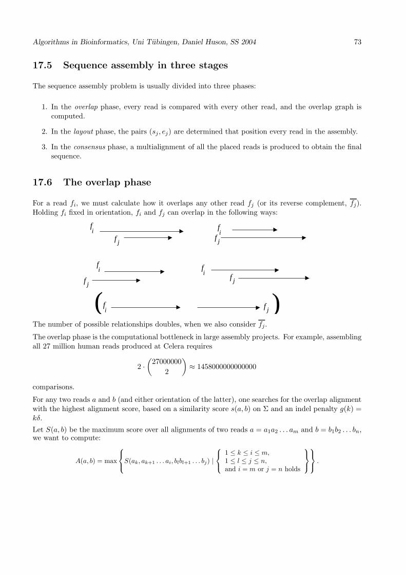
Algorithms in Bioinformatics, Uni Tubingen, Daniel Huson, SS 2004 73
17.5 Sequence assembly in three stages
The sequence assembly problem is usually divided into three phases:
1. In the overlap phase, every read is compared with every other read, and the overlap graph iscomputed.
2. In the layout phase, the pairs (sj , ej) are determined that position every read in the assembly.
3. In the consensus phase, a multialignment of all the placed reads is produced to obtain the finalsequence.
17.6 The overlap phase
For a read fi, we must calculate how it overlaps any other read fj (or its reverse complement, fj).Holding fi fixed in orientation, fi and fj can overlap in the following ways:
fi
f j
fi
f j
fi
fi
fi
f j
f j
f j )(The number of possible relationships doubles, when we also consider fj.
The overlap phase is the computational bottleneck in large assembly projects. For example, assemblingall 27 million human reads produced at Celera requires
2 ·(
27000000
2
)
≈ 1458000000000000
comparisons.
For any two reads a and b (and either orientation of the latter), one searches for the overlap alignmentwith the highest alignment score, based on a similarity score s(a, b) on Σ and an indel penalty g(k) =kδ.
Let S(a, b) be the maximum score over all alignments of two reads a = a1a2 . . . am and b = b1b2 . . . bn,we want to compute:
A(a, b) = max
S(ak, ak+1 . . . ai, blbl+1 . . . bj) |
1 ≤ k ≤ i ≤ m,1 ≤ l ≤ j ≤ n,and i = m or j = n holds
.

74 Algorithms in Bioinformatics, Uni Tubingen, Daniel Huson, SS 2004
17.7 Overlap alignment
This is a standard pairwise alignment problem (similar to local alignment, except we don’t have a 0in the recursion) and we can use dynamic programming to compute:
A(i, j) = maxS(ak, ak+1 . . . ai, blbl+1 . . . bj) | 1 ≤ k ≤ i and 1 ≤ l ≤ j.
Algorithm (Overlap alignment)Input: a = a1a2 . . . an and b = b1b2 . . . bm, s(·, ·) and δOutput: A(i, j)begin
A(0, j) = A(i, 0) ← 0 for i = 1, . . . , n, j = 1, . . . ,mfor i = 1, . . . , n:
for j = 1, . . . ,m:
A(i, j) ← max
A(i− 1, j) − δ,A(i, j − 1)− δ,A(i− 1, j − 1) + s(ai, bi)
end
Runtime is O(nm).
Given two reads a = a1a2 . . . am and b = b1b2 . . . bn. For the matrix A(i, j) computed as above, set
(p, q) := arg maxA(i, j) | i = m or j = n.
There are two cases:p = m or q = n
The trace-back paths look like this:
1001
A(i,j)
am
n
p
qb
or
1001
A(i,j)
am
n
b
p
q
The alignments look like this:a
b or
a
b
17.8 Faster overlap detection
Dynamic programming is too slow for large sequencing projects. Indeed, it is wasteful, as in assembly,only high scoring overlaps with more than 96% identity, say, play a role.
One can use a seed and extend approach (as used in BLAST):
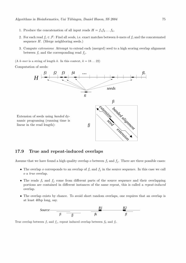
Algorithms in Bioinformatics, Uni Tubingen, Daniel Huson, SS 2004 75
1. Produce the concatenation of all input reads H = f1f2 . . . fL.
2. For each read fi ∈ F : Find all seeds, i.e. exact matches between k-mers of fi and the concatenatedsequence H. (Merge neighboring seeds.)
3. Compute extensions: Attempt to extend each (merged) seed to a high scoring overlap alignmentbetween fi and the corresponding read fj.
(A k-mer is a string of length k. In this context, k = 18 . . . 22)
Computation of seeds:
H...f1 f2 f3 f4 fL
fi
seeds
Extension of seeds using banded dy-namic programing (running time islinear in the read length): fj
banded alignment
seed
extension
extension
fi
17.9 True and repeat-induced overlaps
Assume that we have found a high quality overlap o between fi and fj. There are three possible cases:
• The overlap o corresponds to an overlap of fi and fj in the source sequence. In this case we callo a true overlap.
• The reads fi and fj come from different parts of the source sequence and their overlappingportions are contained in different instances of the same repeat, this is called a repeat-inducedoverlap.
• The overlap exists by chance. To avoid short random overlaps, one requires that an overlap isat least 40bp long, say.
fjfiSource
fk fl
R1 R2
True overlap between fi and fj , repeat induced overlap between fk and fl.

76 Algorithms in Bioinformatics, Uni Tubingen, Daniel Huson, SS 2004
17.10 Avoiding repeat-induced overlaps
To avoid the computation of repeat-induced overlaps, one strategy is to only consider seeds in theseed-and-extend computation whose k-mers are not contained inside a repeat. In this way we canensure that any computed overlap has a significant unique part.
There are two strategies for this:
• Screening known repeats: Each read is aligned against a database of known repeats, i.e. usingRepeatmasker. Portions of reads that match a known repeat are labeled repetitive.
• De novo screening: Choose k = 20, say. Let H denote the concatenation of all reads. Foreach k-mer contained in H, we determine how many times it occurs in H and then label thosek-mers (and their occurrences in the set of reads) as repetitive, whose number of occurrences isunexpectedly high.
17.11 Celera’s overlapper
The assembler developed at Celera Genomics employs an overlapper than compares up to 32 millionpairs of reads per second.
Overlapping all pairs of 27 million reads of human DNA using this program takes about 10 days,running on about 10-20 four processor machines (Compaq ES40), each with 4GB of main memory.
The input data file is about 50GB. To parallelize the overlap compute, each job grabs as many readsas will fit into 4GB of memory (minus the memory necessary for doing the computation) and thenstreams all 27 million reads against the ones in memory.
17.12 The overlap graph
The overlap phase produces an overlap graph OG, defined as follows: Each read fp ∈ F is representedby a directed edge (sp, ep) from node sp to ep, representing the start and end of fp, respectively. Thelength of such a read edge is simply the length of the corresponding read.
An overlap between fp = fp1fp2 . . . fpmand fq = fq1fq2 . . . fqn
gives rise to an undirected overlap edgee between sp, or ep, and sq, or fq, depending on the orientation of the overlap, e.g.:
j
i
1
sp
eq
ep
sq
mfp
fq
1
n
The label (or “length”) of the overlap edge e is defined to be −1 times the overlap length, e.g.−(m−i+j−1
2 + 1) in the figure.
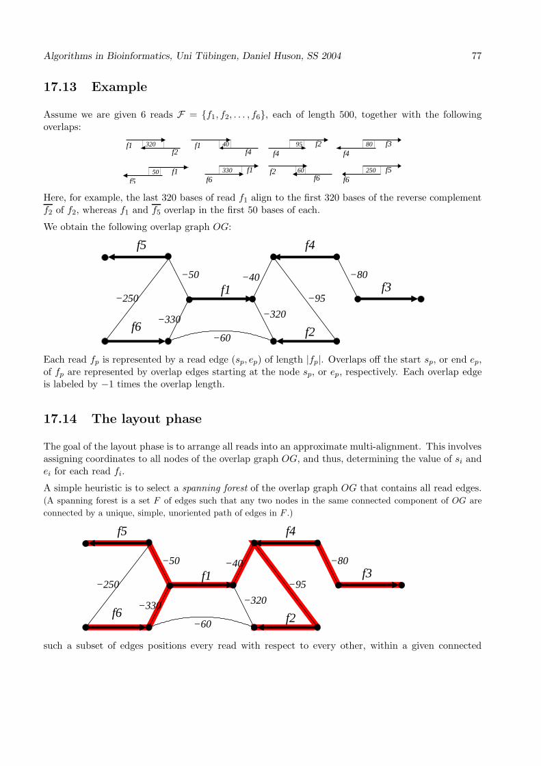
Algorithms in Bioinformatics, Uni Tubingen, Daniel Huson, SS 2004 77
17.13 Example
Assume we are given 6 reads F = f1, f2, . . . , f6, each of length 500, together with the followingoverlaps:
50 f1f5
330
40f1f4
f6f1
320f1f2
95
f4f2
60f6
f2
80
f4f3
250
f6f5
Here, for example, the last 320 bases of read f1 align to the first 320 bases of the reverse complementf2 of f2, whereas f1 and f5 overlap in the first 50 bases of each.
We obtain the following overlap graph OG:
−40f1
f2f6
f3−250
−330
−60
−50
−320
−95
−80
f5 f4
Each read fp is represented by a read edge (sp, ep) of length |fp|. Overlaps off the start sp, or end ep,of fp are represented by overlap edges starting at the node sp, or ep, respectively. Each overlap edgeis labeled by −1 times the overlap length.
17.14 The layout phase
The goal of the layout phase is to arrange all reads into an approximate multi-alignment. This involvesassigning coordinates to all nodes of the overlap graph OG, and thus, determining the value of si andei for each read fi.
A simple heuristic is to select a spanning forest of the overlap graph OG that contains all read edges.(A spanning forest is a set F of edges such that any two nodes in the same connected component of OG are
connected by a unique, simple, unoriented path of edges in F .)
−40f1
f2f6
f3−250
−330
−60
−50
−320
−95
−80
f5 f4
such a subset of edges positions every read with respect to every other, within a given connected

78 Algorithms in Bioinformatics, Uni Tubingen, Daniel Huson, SS 2004
component of the graph:
5004501 730280 950 1410
f5
f1
f6
f4
f2
f3
1830
Such a putative alignment of reads is called a contig.
The spanning tree is usually constructed using a greedy heuristic in which the overlap edges are chosenin decreasing overlap length (i.e., increasing edge “length”).
−40f1
f2f6
f3−250
−330
−60
−50
−320
−95
−80
f5 f4
17.15 Repeats and the layout phase
Consider the following situation:
R
f1f2
f3
f4f5
f7
f6
two copy repeat
reads
sourceR’
This gives rise to the following overlap graph:
f1
f2
f3
f4
f5
f6
f7

Algorithms in Bioinformatics, Uni Tubingen, Daniel Huson, SS 2004 79
Consider this spanning tree:
f
f1
f2
f3
f4
f5
f6
f7
e
A layout produced using the edge e or f does not reflect the true ordering of the reads and the obtainedcontig is called misassembled:
f1f2
f3
f4
f5
f7
f6
e
However, avoiding the repeat-induced edges e and f , one obtains a correct layout:f1
f2f3
f4f5
f7
f6
Note that neither of the two layouts is “consistent” with all overlap edges in the graph.
17.16 Unitigging
The main difficulty in the layout phase is that we can’t distinguish between true overlaps and repeat-induced overlaps. The latter produce “inconsistent” layouts in which the coordinate assignment in-duces overlaps that are not reflected in the overlap graph (e.g., reads f4 and f7 in the example above).
Thus, the layout phase proceeds in two stages:
1. Unitigging: First, all uniquely assemblable contigs are produced, as just described. These arecalled unitigs.
2. Repeat resolution: Then, at a later stage, one attempts to reconstruct the repetitive sequencethat lies between such unitigs.
Reads are sampled from a source sequence that contains repeats:
reads:
source:
repeats
Reads that form consistent chains in the overlap graph are assembled into unitigs and the remaining“repetitive” reads are processed later:

80 Algorithms in Bioinformatics, Uni Tubingen, Daniel Huson, SS 2004
layouts
untigs:
:
reads in repeats:
17.17 Unique unitigs
As defined above, a “unitig” is obtained as a chain of consistently overlapping reads. However, aunitig does not necessarily represent a segment of unique source sequence. For example, its reads maycome from the interior of different instances of a long (many copy) repeat:
reads:
source: R R’ R"
non−unique unitigunique unitig
Non-unique unitigs can be detected by virtue of the fact that they contain significantly more readsthan expected.
17.18 Identifying unique unitigs
Let R be the number of reads and G the estimated length of the source sequence. For a unique unitigof approximate length ρ, the probability of the unitig containing k reads, that is, of seeing k− 1 startpositions in the interval of length ρ, is
e−cck
k!, with c :=
ρR
G,
if the unitig is not oversampled, ande−2c(2c)k
k!,
if the unitig is the result of collapsing two repeats.(see Mike Waterman’s book, page 148, for details)
The arrival statistic used to identify unique unitigs is the (natural) log of the ratio of these twoprobabilities,
c− k log 2.
A unitig is called unique, if it’s arrival statistic has a positive value of 10 or more, say.

Algorithms in Bioinformatics, Uni Tubingen, Daniel Huson, SS 2004 81
17.19 Mate-pairs
Fragment assembly of reads produces contigs, whose relative placement and orientation with respectto each other is unknown.
Recall that modern shotgun sequencing protocols employ a so-called double barreled shotgun. Thatis, longer clones of a given fixed length are sequenced from both ends and one obtains a pair of reads,a mate-pair, whose relative orientation and mean µ (and standard deviation σ of) length are known:
(µ,σ)Typical clone lengths are µ = 2kb, 10kb, 50kb or 150kb. For clean data, σ ≈ 10% of µ. Mate-pairmismatching is a problem and can effect 10− 30% of all pairs.
17.20 Scaffolding
Consider two reconstructed contigs. If they correspond to neighboring regions in the source sequence,then we can expect to see mate-pairs that span the gap between them:
c1 c2
Such mate-pairs determine the relative orientation of both contigs, and we can compute a mean andstandard deviation for the gap between them. In this case, the contigs are said to be scaffolded:
17.21 Determining the distance between two contigs
Given two contigs c1 and c2 connected by mate-pairs m1,m2, . . . ,mk. Each mate-pair gives an esti-mation of the distance between the two contigs.
These estimations can viewed as independent measurements (l1, σ1), (l2, σ2), . . . (lk, σk) of the distanceD between the two contigs c1 and c2. Following standard statistical practice, they can be combinedas follows:
Define p :=∑ li
σ2i
and q =∑ 1
σ2i
. We set the distance between c1 and c2 to
D :=p
q, with standard deviation σ :=
1√q.
Here is an example:

82 Algorithms in Bioinformatics, Uni Tubingen, Daniel Huson, SS 2004
,
,,
,
D,σ
l1σ1
l2σ2
l3 σ3
l4 σ4 2k
10k
10k
2k mate pair
mate pair
mate pair
mate pair
It is possible that the mate-pairs between two contigs c1 and c2 lead to significantly different estimationsof the distance from c1 and c2. In practice, only mate-pairs that confirm each other, i.e. whoseestimations are within 3σ of each other, say, are considered together in a gap estimation.
17.22 The significance of mate-pairs
Given two contigs c1 and c2. If there is only one mate-pair between the two contigs, then due to thehigh error rates associated with mate-pairs, this is not significant.
If, however, c1 and c2 are unique unitigs, and if there exist two different mate-pairs between the twothat give rise to the same relative orientation and similar estimations of the gap size between c1 andc2, then this the scaffolding of c1 and c2 is highly reliable.
This is because that probability that two false mate-pairs occur that confirm each other, is extremelysmall.
17.23 Example
Let the sequence length be G = 120Mb, for example (Drosophila). For simplicity, assume we have5-fold coverage of mate-pairs, with a mean length of µ = 10kb and standard deviation of σ = 1kb.
Consider a false mate-pair m1 = (f1, f2) with reads f1 and f2. Let N1 and N2 denote the two intervals(in the source sequence) of length 3σ centered at the starts of f1 and f2, respectively. Both havelength 6kb.
Consider a second false mate m2 = (g1, g2) with g1 inside N1. The probability that g2 lies in N2 isroughly
6kb
120Mb=
1
20000.
N1 N2source
f2f1
g1m1
m2
Assume that the reads have length 600. Assume that 10% of all mate-pairs are false. At 5-foldcoverage, the interval N1 is covered by about 5 · 6000
600 = 50 reads, of which ≈ 5 have false mates.

Algorithms in Bioinformatics, Uni Tubingen, Daniel Huson, SS 2004 83
Hence, the probability that m1 is confirmed by some second false mate-pair m2 is
≈ 5 · 1
20000=
1
4000= 0.00025.
17.24 The overlap-mate graph
Given a set of reads F = f1, f2, . . . , fR and let G denote the overlap graph associated with F .
Given one set (or more) Mµ,σ = m1, . . . ,mk of mate-pairs mk = (fi, fj), with mean µ and standarddeviation σ.
Let fi and fj be two mated reads represented by the edges (si, ei) and (sj , ej) in G. We add anundirected mate edge between ei and ej , labeled (µ, σ), to indicate that fi and fj are mates and thusobtain the overlap-mate graph:
−40f1
f2f6
f3−250
−330
−60
−50
−320
−95
−80
f5 f4
f7
f8
(2000,200)
(10000,1000)
17.25 The contig-mate graph
Given a set of F of fragments and a set of assembled contigs C = c1, c2, . . . , ct. A more useful graphis obtained as follows:
Represent each assembled contig ci by a contig edge with nodes si and ei. Then, add mate edgesbetween such nodes to indicate that the corresponding contigs contain fragments that are mates:
,
,,
,
D,σ
l1σ1
l2σ2
l3 σ3
l4 σ4 2k
10k
10k
2k mate pair
mate pair
mate pair
mate pair
Leads to:
,l2 σ2
,l3 σ3,l4 σ4
c1 c2
,l1 σ1

84 Algorithms in Bioinformatics, Uni Tubingen, Daniel Huson, SS 2004
17.26 Edge bundling
Consider two contigs c1 and c2, joined by mate-pair edges m1, . . . ,mk between node e1 and s2, say.Every maximal subset of mutually confirming mate edges is replaced by a single bundled mate edge e,whose mean length µ and standard deviation σ are computed as discussed above. Any such bundlededge is labeled (µ, σ).
(A heuristic used to compute these subsets is to repeatedly bundle the median-length simple mateedge with all mate edges within three standard deviations of it, until all simple mate edges have beenbundled.)
Additionally, we set the weight w(e) of any mate edge to 1, if it is a simple mate edge, and to∑k
i=1w(ei), if it was obtained by bundling edges e1, . . . , ek.
Consider the following graph:
Assuming that mate edges drawn together have similar lengths and large enough standard deviation,edge bundling will produce the following graph:
w=2
w=2
w=3w=4
17.27 Transitive edge reduction
Consider the previous graph with some specific edge lengths:
l=µ= µ=1000
2000
40
µ=4200
1000µ=
e
c1 f
g
c2h c3
The mate edge e gives rise to estimation of the distance from the right node of contig c1 to the leftnode of c3 that is similar to the one obtained by following the path P=(g, c2, h). Based on thistransitivity property we can reduce the edge e on to the path p:

Algorithms in Bioinformatics, Uni Tubingen, Daniel Huson, SS 2004 85
to obtain:
w=3+2w=4+2
w=2
Consider two nodes v and w that are connected by an alternating path P = (m1, b1,m2, . . . ,mk) ofmate-edges (m1,m2, . . .) and contig edges (c1, c2, . . .) from v to w, beginning and ending with a mate-edge. We obtain a mean length and standard deviation for P by setting l(P ) :=
∑
miµ(mi)+
∑
cil(ci)
and σ(P ) :=√
∑
miσ(mi)2.
We say that a mate-edge e from v to w can be transitively reduced on to the path P , if e and Papproximately have the same length, i.e. if |µ(e)− l(P )| ≤ C ·maxσ(e), σ(P ) for some constant C,typically 3. If this is the case, then we can reduce e by removing e from the graph and incrementingthe weight of every mate-edge mi in P by w(e).
In the following, we will assume that any contig-mate graph considered has been edge-bundled and perhaps also
transitively reduced to some degree.
17.28 Happy mate-pairs
Consider a mate-pair m of two reads fi and fj, obtained from a clone of mean length µ and standarddeviation σ:
fi(µ,σ) fj
Assume that fi and fj are contained in the same contig or scaffold of an assembly. We call m happy,if fi and fj have the correct relative orientation (i.e., are facing each other) and are at approximatelythe right distance, i.e., |µ − |si − sj|| ≤ 3σ, say. Otherwise, m is unhappy. Two unhappy mates arehighlighted here:
c1 c2
17.29 Ordering and orientation of the contig-mate graph
Given a collection of contigs C = c1, c2, . . . , ck constructed from a set of reads F = f1, f2, . . . , fR,together with the corresponding mate-pair information M . Let G = (V,E) denote the associatedcontig-mate graph.
An ordering (and orientation) of G (or C) is a map φ : V → N such that |φ(bi)− φ(ei)| = l(ci) for allcontigs ci ∈ C, in other words, an assignment of coordinates to all nodes that preserves contig lengths.
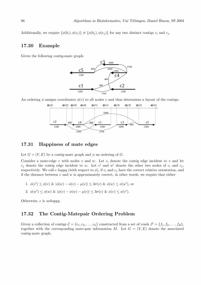
86 Algorithms in Bioinformatics, Uni Tubingen, Daniel Huson, SS 2004
Additionally, we require φ(bi), φ(ei) 6= φ(bj), φ(ej) for any two distinct contigs ci and cj .
17.30 Example
Given the following contig-mate graph:
c4
c2
2700
1000
c1
1500
c5
1500 15002500
900
400
10005000
c3900
An ordering φ assigns coordinates φ(v) to all nodes v and thus determines a layout of the contigs:
(s2)φ φ(s4) (e1)φ (s1)φ (s3)φ (e3)φ (s5)φ(e2)φ (e4)φ (e5)φ
c2 c1 c3 c5c41500
90010001500
2700
5000
1000
2500
900400
1500
17.31 Happiness of mate edges
Let G = (V,E) be a contig-mate graph and φ an ordering of G.
Consider a mate-edge e with nodes v and w. Let ci denote the contig edge incident to v and letcj denote the contig edge incident to w. Let v′ and w′ denote the other two nodes of ci and cj ,respectively. We call e happy (with respect to φ), if ci and cj have the correct relative orientation, andif the distance between v and w is approximately correct, in other words, we require that either
1. φ(v′) ≤ φ(v) & |φ(w) − φ(v)− µ(e)| ≤ 3σ(e) & φ(w) ≤ φ(w′), or
2. φ(w′) ≤ φ(w) & |φ(v) − φ(w) − µ(e)| ≤ 3σ(e) & φ(v) ≤ φ(v′).
Otherwise, e is unhappy.
17.32 The Contig-Matepair Ordering Problem
Given a collection of contigs C = c1, c2, . . . , ck constructed from a set of reads F = f1, f2, . . . , fR,together with the corresponding mate-pair information M . Let G = (V,E) denote the associatedcontig-mate graph.

Algorithms in Bioinformatics, Uni Tubingen, Daniel Huson, SS 2004 87
Problem The Contig-Matepair Ordering Problem is to find an ordering of G that maximizes the sumof weights of happy mate edges.
Theorem The corresponding decision problem is NP-complete.
(The decision problem is: Given a contig-mate graph G, does there exist an ordering of G such thatthe total weight of all happy edges ≥ K?)
17.33 Proof of NP-completeness
Recall: to prove that a problem X is NP-complete one must reduce a known NP-complete problemN to X. In other words, one must show that any instance I of N can be translated into an instanceJ of X in polynomial time such that I has the answer true iff J does.
We will use the following NP-complete problem:
BANDWIDTH: For a given graph G = (V,E) with node set V = v1, v2, . . . , vn and number K, doesthere exist a permutation φ of 1, 2, . . . , n such that for all edges vi, vj ∈ E we have |φ(i)− φ(j)| ≤K? (See Garey and Johnson 1979 for details.)
A graph with bandwidth 4:
Problem is in NP: For a given ordering φ, we can determine whether the number of happy mate-edgesexceeds the given threshold K in polynomial time by simple inspection of all mate edges.
Reduction of BANDWIDTH: Given an instance G = (V,E) of this problem, we construct a contiggraph G′ = (V ′, E′) in polynomial time as follows:
First, set V ′ := V and E′ := E, and let these edges be the mate-edges, setting µ(e) := 1 + K−12 and
σ(e) := K−16 so as to obtain a happy range of [1,K], and w(e) := 1, for every mate-edge e.
Then, for each initial node v ∈ V , add a new auxiliary node v′ to V ′ and join v and v′ by a contigedge of length 0.
The answer to the BANDWIDTH question is true, iff the graph G′ has an ordering φ such that allmate edges in G′ are happy:
A graph G has BANDWIDTH ≤ K⇐⇒
∃ permutation φ such that vi, vj ∈ E implies |φ(i) − φ(j)| ≤ K⇐⇒
∃ ordering φ such that vi, vj ∈ E implies 1 ≤ |φ(i) − φ(j)| ≤ K⇐⇒
∃ ordering φ such that e = vi, vj ∈ E implies µ(e)− 3σ(e) ≤ |φ(i) − φ(j)| ≤ µ(e) + 3σ(e)⇐⇒
all mate-edges of G′ are happy.

88 Algorithms in Bioinformatics, Uni Tubingen, Daniel Huson, SS 2004
17.34 Spanning tree heuristic for the Contig Ordering Problem
An ordering φ that maximizes the number of happy mate edges is a useful scaffolding of the givencontigs.
The simplest heuristic for obtaining an ordering is to compute a maximum weight spanning tree forthe contig-mate graph and use it to order all contigs, similar to the read layout problem.
c1 c2 c3 c4 c5 c6 c7
false mate edge
source
Unfortunately, this method does not work well in practice, as false mate edges lead to incorrectinterleaving of contigs from completely different regions of the source sequence:
c5 c6 c7
c1 c2 c3 c4
17.35 Representing an ordering in the mate-contig graph
By the definition given above, an ordering is an assignment of coordinates to all nodes of the contig-mate graph that corresponds to a scaffolding of the contigs. When we are not interested in the exactcoordinates, then the relative order and orientation of the contigs can be represented as follows:
Given a contig-mate graph G = (V,E). A set S ⊆ E of selected edges is called a scaffolding of G, if ithas the following two properties:
• every contig edge is selected, and
• every node is incident to at most two selected edges.
Thus, a scaffolding of G is a set of non-intersecting selected paths, each representing a scaffolding ofits contained contigs.
The following example contains two chains of selected edges representing scaffolds s1 = (c1, c2, c3, c4)and s2 = (c5, c6, c7):
c1 c2 c3 c4
c5 c6 c7
However, to be able to represent the interleaved scaffolding discussed earlier, we need to add someinferred edges (shown here as dotted lines) to the graph:
c1 c2 c3 c4
c5 c6 c7

Algorithms in Bioinformatics, Uni Tubingen, Daniel Huson, SS 2004 89
17.36 Greedy path-merging
Given a contig-mate graph G = (V,E). The greedy path merging algorithm is a heuristic for solvingthe Contig Ordering Problem. It proceeds “bottom up” as follows, maintaining a valid scaffoldingS ⊆ E:
Initially, all contig edges c1, c2, . . . ck are selected, and none others. At this stage, the graph consistsof k selected paths P1 = (c1), . . . , Pk = (ck).
Then, in ordering of decreasing weight we consider each mate edge e = v,w: If v and w lie in thesame selected path Pi, then e is a chord of Pi and no action is necessary.
If v and w are contained in two different paths Pi and Pj, then we attempt to merge the two pathsto obtain a new path Pk and accept such a merge, only if the increase of H(G), the number of happymate edges, is larger than the increase of U(G), the number of unhappy ones.
17.37 The greedy path-merging algorithm
Algorithm Given a contig-mate graph G. The output of this algorithm is a node-disjoint collectionof selected paths in G, each one defining an ordering of the contigs whose edges it covers.
beginSelect all contig edges.for each mate-edge e in descending order of weight:
if e is not selected:Let v,w denote the two nodes connected by eLet P1 be the selected path incident to vLet P2 be the selected path incident to wif P1 6= P2 and we can merge P1 and P2 (guided by e)
to obtain P :if H(P )− (H(P1) +H(P2)) ≥ U(P )− (U(P1) + U(P2)):
Replace P1 and P2 by Pend
17.38 Merging two paths
Given two selected paths P1 and P2 and a guiding unselected mate-edge e0 with nodes v0 (incident toP1) and w0 (incident to P2). Merging of P1 and P2 is attempted as follows:

90 Algorithms in Bioinformatics, Uni Tubingen, Daniel Huson, SS 2004
(a)
w0
P2
P1
e0h
v0
c11 c12
c21 c22 c23 c25c24
c13 c14
c26
c15
c27
(b)P2
P1
e0 e1
v1
w1
w0g0f0
h
v0
c11
c21 c22
c12
c23 c24
c25
c13
c14
c26 c27
c15
(c)P2
P1
e0 e1
v1w0 w1
e2
w2
v2f1 g1g0f0
h
v0
c15
c27c14c26c13
c25
c24c23
c12
c22
c11
c21
This algorithm returns true, if it successfully produced a new selected path P containing all contigsedges in P1 and P2, and false, if it fails.
Merging proceeds by “zipping” the two paths P1 and P2 together, first starting with e0 and “zipping”to the right. Then, with the edge labeled h now playing the role of e0, zipper to the left. Merging issaid to fail, if the positioning of the “active” contig c1i implies that it must overlap with some contigin P2 by a significant amount, but no such alignment (of sufficiently high quality) exists.
17.39 Example
Here are we are given 5 contigs c1, . . . , c5, each of length l(ci) = 10000:
w=1, µ=12000
w=5,µ=12000
w=1, µ=34000
w=2,µ=1000w=3,µ=1000
w=4,µ=12000
c2
c1
c3
c4
c5
w=1, µ=12000
w=5,µ=12000
w=1, µ=34000
w=2,µ=1000w=3,µ=1000
w=4,µ=12000
c2
c1
c3
c4
c5
w=1, µ=12000
w=5,µ=12000
w=1, µ=34000
w=2,µ=1000w=3,µ=1000
w=4,µ=12000
c2
c1
c3
c4
c5
w=1, µ=12000
w=5,µ=12000
w=1, µ=34000
w=2,µ=1000w=3,µ=1000
w=4,µ=12000
c2
c1
c3
c4
c5
w=5,µ=12000
w=1, µ=34000
w=3,µ=1000
w=4,µ=12000
c2
c1
c3
c4
c5
w=1, µ=12000
w=2,µ=1000
w=5,µ=12000
w=1, µ=34000
w=3,µ=1000
w=4,µ=12000
c2
c1
c3
c4
c5
w=1, µ=12000
w=2,µ=1000
µ~1000µ~1000
The final scaffolding is (c1, c2, c3, c5, c4).

Algorithms in Bioinformatics, Uni Tubingen, Daniel Huson, SS 2004 91
17.40 Repeat resolution
Consider two unique unitigs u1 and u2 that are placed next to each other in a scaffolding, due to aheavy mate edge between them:
u2u1
We consider all non-unique unitigs and singleton reads that potentially can be placed between u1 andu2 by mate edges:
u2u1
Different heuristics are used to explore the corresponding local region of the overlap graph in anattempt to find a chain of overlapping fragments that spans the gap and is compatible with the givenmate-pair information:
u2u1
17.41 Summary
Given a collection F = f1, f2, . . . , fR of reads and mate-pair information, sampled from a unknownsource DNA sequence. Assembly proceeds in the following steps:
1. compute the overlap graph, e.g. using a seed-and-extend approach,
2. construct all unitigs, e.g. using the minimal spanning tree approach,
3. scaffold the unitigs, e.g. using the greedy-path merging algorithm,
4. attempt to resolve repeats between unitigs, and
5. compute a multiple alignment of all reads in a given contig to obtain a consensus sequence forit.
Note that the algorithms for steps (2) and (3) that are used in actual assembly projects are much more sophis-
ticated than ones described in these notes.
17.42 A WGS assembly of human (Celera)
Input: 27 million fragments of av. length 550bp, 70% paired:

92 Algorithms in Bioinformatics, Uni Tubingen, Daniel Huson, SS 2004
5m pairs of length 2kb4m pairs of length 10kb
0.9m pairs of length 50kb0.35m pairs of length 150kb
Celera’s assembler uses approximately the following resources:
Program CPU Max.hours memory
Screener 4800 2-3 days on 10-20 computers 2GBOverlapper 12000 10 days on 10-20 computers 4GBUnitigger 120 4-5 days on a single computer 32GBScaffolder 120 4-5 days on a single computer 32GBRepeatRez 50 Two days on a single computer 32GBConsensus 160 One day on 10-20 computers 2GB
Total: ≈ 18000 CPU hours.
The size of the human genome is ≈ 3Gb. An unpublished 2001 assembly of the 27m fragments hasthe following statistics:
• The assembly consists of 6500 scaffolds that span 2.776Gb of sequence.
• The spanned sequence contains 150, 000 gaps, making up 148Mb in total.
• Of the spanned sequence, 99.0% is contained in scaffolds of size 30kb or more.
• Of the spanned sequence, 98.7% is contained in scaffolds of size 100kb or more.

Algorithms in Bioinformatics, Uni Tubingen, Daniel Huson, SS 2004 89
18 Sequencing From Compomers
This exposition is based on the following sources, which are recommended reading:
• A.E. Ashcroft, An Introduction to Mass Spectrometry,http://www.astbury.leeds.ac.uk/Facil/MStut/mstutorial.htm
• S. Bocker, Sequencing from Compomers: using mass spectrometry for DNA de-novo sequencingof 200+ nt, in Gary Benson and Roderic D.M. Page, editors, 3rd Workshop on Algorithms inBioinformatics (WABI 2003), Volume 2812 of Lecture Notes in Computer Science, pages 476–497.
De-novo sequencing is performed today using electrophoresis-based approaches, based on ideas intro-duced by Sanger in 1977. We will discuss an alternative proposal that would use mass spectrometryto gather sequence data and produce reads of length 200+, if it can be made to work in practice.
18.1 Mass Spectrometry
Mass spectrometers are an analytical tool used for measuring the molecular weight (MW) of a sample.
For large samples such as biomolecules, molecular weights can be measured to within an accuracy of0.01% of the total molecular weight of the sample i.e. within a 4 Daltons (Da, 1 Da = 1
12 mass of acarbon-12 nucleus) error for a sample of 40,000 Da. This is sufficient to allow minor mass changes tobe detected, e.g. the substitution of one amino acid for another, or a post-translational modification.
For small organic molecules the molecular weight can be measured to within an accuracy of 5 ppm(parts-per-million), which is often sufficient to confirm the molecular formula of a compound, and isalso a standard requirement for publication in a chemical journal.
Structural information can be generated using certain types of mass spectrometers, usually tandemmass spectrometers, and this is achieved by fragmenting the sample and analyzing the productsgenerated.
This procedure is useful for the structural elucidation of organic compounds, for peptide or oligonu-cleotide sequencing, and for monitoring the existence of previously characterized compounds in com-plex mixtures with a high specificity by defining both the molecular weight and a diagnostic fragment ofthe molecule simultaneously e.g. for the detection of specific drug metabolites in biological matrices.
18.2 MALDI TOF MS
MALDI TOF MS stands for matrix assisted laser desorption ionization time-of-flight mass spectrom-etry.

90 Algorithms in Bioinformatics, Uni Tubingen, Daniel Huson, SS 2004
(Source: http://www.astbury.leeds.ac.uk/Facil/MStut/mstutorial.htm)
MALDI is based on the bombardment of sample molecules with a laser light to bring about sampleionization. The sample is pre-mixed with a highly absorbing matrix compound for the most consistentand reliable results, and a low concentration of sample to matrix works best. The matrix transformsthe laser energy into excitation energy for the sample, which leads to sputtering of analyte and matrixions from the surface of the mixture.
The time-of-flight analyzer separates ions according to their mass(m)-to-charge(z) (m/z) ratios bymeasuring the time it takes for ions to travel through a field free region known as the flight, or drift,tube. The heavier ions are slower than the lighter ones.
The m/z scale of the mass spectrometer is calibrated with a known sample that can either be analyzedindependently (external calibration) or pre-mixed with the sample and matrix (internal calibration).
MALDI is a “soft” ionization method and so results predominantly in the generation of singly chargedmolecular-related ions regardless of the molecular weight, hence the spectra are relatively easy tointerpret. Fragmentation of the sample ions does not usually occur.
Example Positive ionization MALDI m/z spectrum of the peptide ACTH (clip 18-39; MW 2465.7Da) using cyano-4-hydroxycinnamic acid as matrix:
(Source: http://www.astbury.leeds.ac.uk/Facil/MStut/mstutorial.htm)
18.3 The Partial Cleavage Experiment
Suppose we are given many copies of a target (or sample) DNA molecule of length 100 − 500, andassume (for simplicity) that they are single stranded.

Algorithms in Bioinformatics, Uni Tubingen, Daniel Huson, SS 2004 91
In four separate reactions, one for each base, we cleave the copies of the target using a base-specific(bio-)chemical cleavage reaction (e.g., RNAse A, RNAse T1, uracil-DNA-gylcoslase, pn-bond cleavageand others.)
More precisely, we only perform partial cleavage reactions so that only a certain percentage of thepossible “cut bases” get cut, thus ideally producing a mixture of all fragments obtainable by cuttingthe target sequence at any two cut bases:
(Source: Bocker, 2003)
MALDI TOF mass spectrometry is then applied to the products of each of the four partial cleavageexperiments in turn, producing four sample spectra that correlate mass and signal intensity of sampleparticles. Each is analyzed to extract a list of signal peaks with masses and intensities:
(Source: Bocker, 2003)
The four nucleotides have different weights and so each peak in such a spectrum corresponds to afragment of a specific composition of bases.
Indeed, given the measured weight W of a fragment f , and the different molecular weights ω(A),ω(C), ω(G) and ω(T ) of the four types of nucleotides, we can easily compute the base-composition ofthe fragment in O(|f |3) steps. (Exercise)
The key idea is to determine the precise sequence of the target molecule as the (hopefully unique)sequence whose calculated spectrum is the same as the measured one.
This is a difficult problem, for two reasons:
• given only the base-compositions of the fragments, the problem of determining a possible targetsequence is NP-hard, and
• MS does not work well for sequences longer than ≈ 25 nt.
It has been used in situations such as in pathogen identification in which information on the targetsequence is already known.
18.4 Some Practical Observations
1. Current MS can only detect modules of weight ≤ 8000 Dalton,
2. MS can show an inaccuracy of 1− 2 Da in high-throughput,

92 Algorithms in Bioinformatics, Uni Tubingen, Daniel Huson, SS 2004
3. MS spectra are noisy and so low-intensity signals are hard to identify,
4. for a fixed cleavage reaction, different compositions can have nearly identical masses,
5. partial cleavage suffers from exponential decay, so long fragments will be difficult to detect, and
6. a small number of the terminal bases of the target are often known in advance.
18.5 The Composer Spectrum
Let s = s1 . . . sn be a string over the alphabet Σ. We denote the number of (non-overlapping)occurrences of a string x in s by:
ordx(s) = maxk | there exist t0, . . . , tk ∈ Σ∗ with s = t0xt1x . . . xtk.So, x is a substring of s iff ordx(s) > 0.
For two string s, x ∈ Σ∗ we define the string spectrum S(s, x) of s by:
S(s, x) = y ∈ Σ∗ | there exist a, b ∈ Σ∗ with s ∈ yxb, axyxb, axy ∪ s,the set of all substrings of s that are bounded by x or by the ends of s.
In the following, we will call s a sample string, x a cut-string and the elements of S(s, x) the fragmentsof s (under x).
Example Consider Σ = 0, A, C, G, T, 1, where 0 and 1 are only used to denote the start and end ofthe sample string. Let
s = 0ACATGTG1 and x = T.
Then we have:S(s, x) = 0ACA, G, G1, 0ACATG, GTG1, 0ACTGTG1.
We introduce the characters 0 and 1 to reduce symmetry, see observation (6) above.
A compomer is a map c : Σ→ N≥0 that records the composition of a fragment of DNA, which we will
often write asc = (AiCjGkTl),
with i = c(A), j = c(C), k = c(G) and l = c(T), sometimes omitting the letters 0 and 1 and symbolswith zero values.
The function comp maps every sequence s ∈ Σ∗ to its compomer by counting the number of charactersof each type in s:
comp(s) : Σ→ N, σ 7→ c(σ) = |1 ≤ i ≤ |s| : si = σ|.
Given a sample sequence s and cut string x, the compomer spectrum C(s, x) consists of all compomersof all fragments in the string spectrum S(s, x):
C(s, x) = comp(S(s, x)) = comp(y) : y ∈ S(s, x).
For the example s = 0ACATGTG1 we have:
C(s, T) = 0A2C1, G1, G11, 0A2C1G1T1, G2T11, 0A2C1G2T21.

Algorithms in Bioinformatics, Uni Tubingen, Daniel Huson, SS 2004 93
18.6 Reconstruction from Complete Compomer Spectra
We can now formulate the Reconstruction from Complete Compomer Spectra (RCCS) problem:
For an unknown string s and a set of know cut strings X, can we uniquely reconstruct sfrom its compomer spectra C(S, x), x ∈ X?
Note that the problem is trivial, if there exist characters 0 and 1 that uniquely denote the start and endof the sample string. Then, for suitable X, e.g. X = Σ1 \ 0, 1, the subsets c ∈ C(s, x) | c(0) = 1,x ∈ X, are sufficient to reconstruct s. (We use Σi ⊂ Σ∗ to denote all substrings of length i.)
Unfortunately, this approach will fail when applied to real MS data, due to some of the observationslisted above.
18.7 Reconstruction from k-Compomer Spectra
A consequence of observation (5) is that a fragment f can only be detected by mass spec if it issufficiently short, that is, contains only a small number of cut sites, say at most 4. This leads to thefollowing two definitions:
For a sample string s, cut string x and number k, we define the k-string spectrum of s (of order k) as:
Sk(s, x) = y ∈ S(s, x) : ordx(y) ≤ k.The k-compomer spectrum of s is defined by:
Ck(s, x) = comp(Sk(s, x)) = comp(y) : y ∈ S(s, x), ordx(y) ≤ k.
For the example s = 0ACATGTG1 we calculate:
C0(s, T ) = 0A2C1, G1, G11,C1(s, T ) = C0(s, T ) ∪ 0A2C1G1T1, G2T11, and
C2(s, T ) = C1(s, T ) ∪ 0A2C1G2T21 = C(s, T ).
Under what conditions can we uniquely reconstruct a sample string s from its compomer spectraCk(s, x), x ∈ X?
Example Let Σ = 0, A, B, 1. We cannot uniquely reconstruct the sample string
s = 0BABAAB1
from its complete cleavage compomer spectra C0(s,A) and C0(s,B) because the string
s = 0BAABAB1
leads to the same spectra.
Similarly,s = 0BABABAABAB1
cannot be reconstructed from its compomer spectra C1(s, x) with x ∈ A,B, and one can create suchexamples for every order k.

94 Algorithms in Bioinformatics, Uni Tubingen, Daniel Huson, SS 2004
18.8 False Positive Compomers
The Reconstruction from k-Compomer Spectra problem suffers from the difficulty that the resultinganswer is not necessarily unique.
An additional problem is that due to Observations (2) and (4), transforming a mass spectrum intoa set of compomers will introduce many false positive compomers, since there is usually only onecompomer that actually corresponds to an observed peak, but many that have a very similar weight.Also, Observation (3) can add to the problem.
To address the problem of false positives, a proposed solution should not be required to explain allobserved compomers.
18.9 Sequencing From Compomers (SFC) Problem
We now formulate the Sequencing From Compomers (SFC) Problem:
For a fixed order k, let X ⊆ Σ∗ be a set of cut strings and, for each x ∈ X, let Cx be acompomer set. Let S ⊆ Σ∗ be a set of sample string candidates. Find all strings s ∈ Sthat satisfy Ck(s, x) ⊆ Cx for all x ∈ X.
Note that the SFC problem has some trivial solutions if we allow S = Σ∗, for example, s = ǫ alwayssatisfies the inclusion conditions. So, S should be chosen to exclude such trivial solutions.
Note that even a small number of compomers can lead to an exponential number of strings, for a givenfixed string length:
For example, let
• Σ = A,B,
• k = 0,
• S = Σn for some n ∈ N,
• X = Σ1, and
• CA = B1 and CB = A1, A2.
Note that every string s ∈ S that is an arbitrary concatenation
s0s1s2 . . . sk with s0 ∈ A,AA and sj ∈ BA,BAA
for j = 1, . . . , k satisfies the conditions
C0(s,A) ⊆ CA and C0(s,B) ⊆ CB.

Algorithms in Bioinformatics, Uni Tubingen, Daniel Huson, SS 2004 95
18.10 The undirected sequencing graph
To address the SFC problem of order k = 1, we introduce the undirected sequencing graph.
Let C be an arbitary set of compomers over Σ. For each single-nucleotide cut string x ∈ Σ1, we definethe undirected sequencing graph Gu(C, x) = (V,E) as follows:
• the vertex set V consists of all compomers c ∈ C such that c(x) = 0 holds, and
• the edge set E consists of those v,w ⊆ V that satisfy:
v + comp(x) + w ∈ C,
where v and w are not required to be distinct.
A sequence p = (p0, p1, . . . , pr) of nodes pi ∈ V is called a walk in G = (V,E), if pi−1, pi ∈ E for alli = 1, . . . , r.
Example For Σ = 0, A,C,G, T, 1, s = 0CTAATCATAGTGCTG1, and x = T , the compomerspectrum of order 1 is:
C := C1(s, T ) = 0C1, 0A2C1T1, A2, A3C1T1, A1C1,A2C1G1T1, A1G1, A1C1G2T1, C1G1, C1G2T11, G11.
The resulting graph Gu(C, T ) is:
We say that a string s ∈ Σ∗ is 1-compatible with a compomer set C under x, if C1(s, x) ⊆ C holds. Inthis case s is a solution to the SFC problem of order 1 with respect to x.
We say that s is compatible with a walk p = (p0, . . . , pr) in Gu(C, x), if there exist strings s0, . . . , sr ∈ Σ∗
such thats = s0xs1xs2x . . . xsr,
with comp(sj) = pj for j = 0, . . . , r. Such a set of strings s0, . . . , sr is called an x-partitioning of s, ifadditionally, ordx(sj) = 0 for all j = 0, . . . , r.
For x ∈ Σ1, there exists exactly one x-partitioning of s.
In the above example, the walk (0C1, A2, A1C1, A1G1, C1G1, G11) is compatible with the in-put sequence s = 0CTAATCATAGTGCTG1. But also sequences like OCTATCGTG1 or0CTAATCGTGATGCTG1 are compatible with walks in Gu(C, T ).
We have the following result:

96 Algorithms in Bioinformatics, Uni Tubingen, Daniel Huson, SS 2004
Lemma Let s ∈ Σ∗ be a string and C a set of compomers over Σ. Then, s is 1-compatible with Cunder x ∈ Σ1 iff there exists a walk p in Gu(C, x) such that s is compatible with p. Morover, p isunique.
Thus, an algorithm to solve the SFC problem can be based on the following:
For every walk p of a sequencing graph Gu(C, x) there exists one or more sequences s ∈ Σ∗
that are compatible with p, and therefore are 1-compatible with C.

Algorithms in Bioinformatics, Uni Tubingen, Daniel Huson, SS 2004 95
19 DNA arrays
This exposition is based on the following sources, which are recommended reading:
1. M.B. Eisen, P.T. Spellman, P.O. Brown and D. Botstein, Cluster analysis and display of genome-wide expression patterns, PNAS, 95:14863-14868, 1998.
2. Pavel Penzer, Computational Molecular biology - an algorithmic approach, MIT Press, 2000,chapter 5.
3. Ron Shamir, Analysis of Gene Expression Data, lectures 1 and 4, 2002.
• Also known as: biochips, DNA chips, oligo arrays, DNA microarrays or gene arrays.
• An array is an orderly arrangement of (spots of) samples.
• Samples are either DNA or DNA products.
• Each spot in the array contains many copies of the sample.
• Array provides a medium for matching known and unknown DNA samples based on base-pairing(hybridization) rules and for automating the process of identifying the unknowns.
• Sample spot size in microarray less than 200 microns and an array contains thousands of spots.
• Microarrays require specialized robotics and imaging equipment.
• High-throughput biology: a single DNA chip can provide information on thousands of genessimultaneously.
19.1 Two possible formats
We are given an unknown target nucleic acid sample and the goal is to detect the identity and/orabundance of its constituents using known probe sequences. Single stranded DNA probes are calledoligo-nucleotides or oligos.
There are two different formats of DNA chips:
• Format I: The target (500-5000 bp) is attached to a solid surface and exposed to a set ofprobes, either separately or in a mixture. The earliest chips where of this kind, used for oligo-fingerprinting.
• Format II: An array of probes is produced either in situ or by attachment. The array is thenexposed to sample DNA. Examples are oligo-arrays and cDNA microarrays.
In both cases, the free sequence is fluorescently or radioactively labeled and hybridization is used todetermine the identity/abundance of complementary sequences.

96 Algorithms in Bioinformatics, Uni Tubingen, Daniel Huson, SS 2004
19.2 Oligo arrays C(l)
The simplest oligo array C(l) consists of all possible oligos of length l and is used e.g. in sequencingby hybridization (SBH).
C(4) A A A A T T T T G G G G C C C CA T G C A T G C A T G C A T G C
AAATAGACTATTTGTC
GAGTGGGCCACTCGCC
Example: oligo at : TCGA
19.3 cDNA microarrays
The aim of this technology is to analyze the expression of thousands of genes in a single experimentand provides measurements of the differential expression of these genes.
Here, each spot contains, instead of short oligos, identical cDNA clones, which represents a gene.(Such complementary DNA is obtained by reverse transcription from some known mRNA.) The targetis the unknown mRNA extracted from a specific cell. As most of the mRNA in a cell is translatedinto a protein, the total mRNA in a cell represents the genes expressed in the cell.
Since cDNA clones are much longer than the short oligos otherwise used, a successful hybridizationwith a clone is an almost certain match. However, because an unknown amount of cDNA is printedat each spot, one cannot directly associate the hybridization level with a transcription level and socDNA chips are limited to to comparisons of a reference extract and a target extract.
19.4 Affymetrix chips
Affymetrix produces oligo arrays with the goal of capturing each coding region as specifically aspossible. The length of the oligos is usually less than 25 bases. The density of oligos on a chip can bevery high and a 1cm × 1cm chip can easily contain 100 000 types of oligos.

Algorithms in Bioinformatics, Uni Tubingen, Daniel Huson, SS 2004 97
The chip contains both “coding” oligos and “control” oligos, the former corresponding to perfectmatches to known targets and the controls corresponding to matches with one perturbed base.
When reading the chip, hybridization levels at controls are subtracted from the level of match probesto reduce the number of false positives. Actual chip designs use 10 match- and 10 mismatch probesfor each target gene.
Today, Affymetrix offers chips for the entire (known) human or yeast genomes.
19.5 Oligo fingerprinting
Format I chips were the first type used, namely for oligo fingerprinting which is, in a sense, the oppositeto what Affymetrix chips do. Such a chip consists of a matrix of target DNA and is exposed to asolution containing many identical oligos.
After the positions in the matrix have been recorded at which hybridization of the tagged oligos hasoccurred, the chip can be heated to separate the oligos from the target DNA and the experiment canbe repeated with a different type of oligo.
Finally, we obtain a data matrix M , with each row representing a specific target DNA from the matrixand each column representing an oligo probe.
Example: cDNA’s extracted from a tissue. Cluster cDNA’s according to their fingerprints and thensequence representatives from each cluster to obtain a sequence that identifies the gene.
19.6 Manufacturing oligo arrays
1. Start with a matrix created over a glass substrate.
2. Each cell contains a growing “chain” of nucleotides that ends with a terminator that preventschain extension.
3. Cover the substrate with a mask and then illuminate the uncovered cells, breaking the bondsbetween the chains and their terminators.
4. Expose the substrate to a solution of many copies a specific nucleotide base so that each of theunterminated chains is extended by one copy of the nucleotide base and a new terminator.
5. Repeat using different masks.

98 Algorithms in Bioinformatics, Uni Tubingen, Daniel Huson, SS 2004
Exposure to light replaces the terminators by hydrogen bonds (1–2), and (3) bonds forms with nucleotide bases
provided in a solution, and then the process is repeated with a different base (4–6).
19.7 Experiment with a DNA chip
Labeled RNA molecules are applied to the probes on the chip, creating a fluorescent spot where hybridization
has occurred.
19.8 Functional genomics
With the sequencing of more and more genomes, the question arises of how to make use of this data.One area that is now opening up is functional genomics, the understanding of the functionality ofspecific genes, their relations to diseases, their associated proteins and their participation in biologicalprocesses.

Algorithms in Bioinformatics, Uni Tubingen, Daniel Huson, SS 2004 99
The functional annotation of genes is still at an early stage: e.g., for the plant Arabidopsis (whosesequence was recently completed), the functions of 40% of the genes are currently unknown.
Functional genomics is being addressed using high-throughput methods: global gene expression pro-filing (“transcriptome analysis”) and wide-scale protein profiling (“proteome analysis”).
19.9 Gene expression
The existing methods for measuring gene expression are based on two biological assumptions:
1. The transcription level of genes indicates their regulation: Since a protein is generated from agene in a number of stages (transcription, splicing, synthesis of protein from mRNA), regulationof gene expression can occur at many points. However, we assume that most regulation is doneonly during the transcription phase.
2. Only genes which contribute to organism fitness are expressed, in other words, genes that areirrelevant to the given cell under the given circumstances etc. are not expressed.
Genes affect the cell by being expressed, i.e. transcribed into mRNA and translated into proteins thatreact with other molecules.
From the pattern of expression we may be able to deduce the function of an unknown gene. Thisis especially true, if the pattern of expression of the unknown gene is very similar to the pattern ofexpression of a gene with known function.
Also, the level of expression of a gene in different tissues and at different stages is of significant interest.
Hence, it is highly interesting to analyze the expression profile of genes, i.e. in which tissues and atwhat stages of development they are expressed.
19.10 cDNA Clustering
It is not easy to determine which genes are expressed in each tissue, and at what level:
An average tissue contains more than 10 000 expressed genes, and their expression levels can vary bya factor of 10 000. Hence, we need to extract more than 105 transcripts per tissue. There are about100 different types of tissue in the body and we are interested in comparing different growth stages,disease stages etc., and so we should analyze more than 1010 transcripts.
⇒ Sequencing all cDNA’s is infeasible and we need cheap, efficient and large scale methods.
19.11 Representation of gene expression data
Gene expression data is represented by a raw data matrix R, where each row corresponds to one geneand each column represents one tissue or condition. Thus, Rij is the expression level for gene i incondition j. The values can be ratios, absolute values or distributions.

100 Algorithms in Bioinformatics, Uni Tubingen, Daniel Huson, SS 2004
Before it is analyzed, the raw data matrix is preprocessed to compute a similarity or distance matrix.
j
conditions
expressionlevels
"raw data"
3
2
4
...
1ge
nes
i
1 2 3 ...
DijRij
j
matrix
genes
i
1
2
3
4
...
1 2 3 ...
gene
s
distance
19.12 Clustering
The first step in analyzing gene expression data is clustering.
Clustering methods are used in many fields. The goal in a clustering problem is to group elements (inour case genes) into clusters satisfying:
1. Homogeneity: Elements inside a cluster are highly similar to each other.
2. Separation: Elements from different clusters have low similarity to each other.
There are two types of clustering methods:
• Agglomerative methods build clusters by looking at small groups of elements and performingcalculations on them in order to construct larger groups.
• Divisive methods analyze large groups of elements in order to divide the data into smaller groupsand eventually reach the desired clusters.
Why would we want to cluster gene expression data? We assume that:
• Distinct measurements of same genes cluster together.
• Genes of similar function cluster together.
• Many cluster-function specific insights are gained.
19.13 Hierarchical clustering
This approach attempts to place the input elements in a tree hierarchy structure in which distancewithin the tree reflects element similarity.
To be precise, the hierarchy is represented by a tree and the actual data is represented by the leavesof the tree. The tree can be rooted or not, depending on the method used.

Algorithms in Bioinformatics, Uni Tubingen, Daniel Huson, SS 2004 101
Distance matrix → Dendrogram
gene 1 2 3 4
1 0 3 5 72 3 0 5 73 5 5 0 74 7 7 7 0
37 5
gene 3
gene 4
gene 2
gene 1
19.14 Average linkage
Average linkage is similar to Neighbor-Joining, except that when computing the new distances ofcreated clusters, the sizes of clusters that are merged are taken into consideration. This algorithm wasdeveloped by Lance and Williams (1967) and Sokal and Michener (1958).
1. Input: The distance matrix Dij , initial cluster sizes nr.
2. Iteration k: The same as in NJ, except that the distance from a new element t is defined by:
Dit := Dti :=nr
nr + nsDir +
ns
nr + nsDis
19.15 Non-Hierarchical clustering
Given a set of input vectors. For a given clustering P of them into k clusters, let EP :=∑
c
∑
v∈c D(v, zc) denote the solution cost function, where zc is the centroid (average vector) of thecluster c and D(v, zc) is the distance from v to zc.
The k-means clustering due to Macqueen (1965) operates as follows:
1. Initialize an abitrary partition P into k clusters.
2. For each cluster c and element e:Let EP (c, e) be the cost of the solution if e is moved to c.
3. Pick c, e so that EP (c, e) is minimum.
4. Move e to c, if it improves EP .
5. Repeat until no further improvement is achieved.
19.16 Application to fibroblast cells
Eisen et al. (1998) performed a series of experiments on real gene expression data. One goal wasto check the growth response of starved human fibroblast cells, which were then given serum. Theexpression level of about n = 8600 genes were monitored over Ncond = 13 time points.

102 Algorithms in Bioinformatics, Uni Tubingen, Daniel Huson, SS 2004
The original data of test to reference ratios was first log transformed, and then normalized to havemean 0 and variance 1. Let Nij denote these normalized levels. A similarity matrix was constructedfrom Nij as follows:
Skl :=
∑nj=1NkjNjl
Ncond
,
where Ncond is the number of conditions checked.
The average linkage method was then used to generate the following tree:
The Dendrogram resulting from the starved human fibroblast cells experiment. Five major clusters can be seen,
and many non clustered genes. The cells in the five groups server similar functions: (A) cholesterol bio-synthesis,
(B) the cell cycle, (C) the immediate-early response, (D) signaling and angiogenesis, and (E) wound healing
and tissue remodeling.
(Color scale red-to-green corresponds to higher-to-lower expression level than in the control state.)
19.17 Testing the significance of the clusters
A standard method for testing the significance of clusters is to randomly permute the input data indifferent ways.
Original expression data (1), clustered data (2), and the results of clustering after random permutations within

Algorithms in Bioinformatics, Uni Tubingen, Daniel Huson, SS 2004 103
rows (3), within columns (4) and within both (5).
19.18 Sequencing by Hybridization (SBH)
Originally, the hope was that one can use DNA chips to sequence lage unknown DNA fragments usinga large array of short probes:
1. Produce a chip C(l) spotted with all possible probes of length l (l = 8 in the first SBH papers),
2. Apply a solution containing many copies of a fluorescently labeled DNA target fragment to thearray.
3. The DNA fragments hybridize to those probes that are complementary to substrings of lengthl of the fragment
4. Detect probes that hybridize with the DNA fragment and obtain the l-tuple composition of theDNA fragment
5. Apply a combinatorial algorithm to reconstruct the sequence of the DNA target from the l-tuplecomposition
19.19 The Shortest Superstring Problem
SBH provides information of the l-tuples present in a target DNA sequence, but not their positions.Suppose we are given the spectrum S of all l-tuples of a target DNA sequence, how do we constructthe sequence?
This is a special case of the Shortest Common Superstring Problem (SCS): A superstring for a givenset of strings s1, s2, . . . , sm is a string that contains each si as a substring. Given a set of strings,finding the shortest superstring is NP-complete.
Define overlap(si, sj) as the length of a maximal prefix of sj that matches a suffix of si. The SCSproblem can be cast as a Traveling Salesman Problem in a complete directed graph G with m verticess1, s2, . . . , sm and edges (si, sj) of length −overlap(si, sj).
19.20 The SBH graph
SBH corresponds to the special case in which all substrings have the same length l. We say that twoSBH probes p and q overlap, if the last l − 1 letters of p coincide with the first l − 1 of q.
Given the spectrum S of a DNA fragment, construct the directed graph H with vertex set S and edgeset
E = (p, q) | p and q overlap.
There exists a one-to-one correspondence between paths that visit each vertex of H at least once andthe DNA fragments with the spectrum S.

104 Algorithms in Bioinformatics, Uni Tubingen, Daniel Huson, SS 2004
19.21 Example of the SBH graph
Vertices: l tuples of the spectrum S, edges: overlapping l-tuples:
ATG AGG TGC TCC GTC GGT GCA CAGS =
H
The path visiting all vertices corresponds to the sequence reconstruction ATGCAGGTCC.
A path that visits all nodes of a graph exactly once is called a Hamiltonian path. Unfortunately, theHamiltonian Path Problem is NP-complete, so for larger graphs we cannot hope to find such paths.
19.22 Second example of the SBH graph
S =
H
ATG TGCTGG GTG GGC GCA GCG CGT
This example has two different Hamiltonian paths and thus two different reconstructed sequences:
ATGCGTGGCA ATGGCGTGCA
19.23 Euler Path
Leonard Euler wanted to know whether there exists a path that uses all seven bridges in Konigsbergexactly once:

Algorithms in Bioinformatics, Uni Tubingen, Daniel Huson, SS 2004 105
Kneiphoff island
Pregel river
Birth of graph theory...
19.24 SBH and the Eulerian Path Problem
Let S be the spectrum of a DNA fragment. We define a graph G whose set of nodes consists of allpossible (l − 1)-tuples.
We connect one l − 1-tuple v = v1 . . . vl−1 to another w = w1 . . . wl−1 by a directed edge (v,w), ifthe spectrum S contains an l-tuple u with prefix v and suffix w, i.e. such that u = v1 . . . vl−1w1 =vl−1w1 . . . wl−1.
Hence, in this graph the probes correspond to edges and the problem is to find a path that visits alledges exactly once, i.e., an Eulerian path.
Finding all Eulerian paths is simple to solve.
(To be precise, the Chinese Postman Problem (visit all edges at least once in a minimal tour) can be efficiently
solved for directed or undirected graphs, but not in a graph that contains both directed and undirected edges.)
AT
GT CG
GCCA
GG
TG
S = CGTGTG, GGC, GCA, GCG,ATG, TGG, TGC,
ATG
GCA
GC
G
GT
G
GCT
GGC
TGG
TGC
Vertices represent (l− 1)-tuples, edges correspond to l-tuples of the spectrum. There are two differentsolutions:

106 Algorithms in Bioinformatics, Uni Tubingen, Daniel Huson, SS 2004
AT
GT CG
GCCA
GG
TG AT
GT CG
GCCA
GG
TG
ATGGCGTGCA ATGCGTGGCA
19.25 Eulerian graphs
A directed graph G is called Eulerian, if it contains a cycle that traverses every edge of G exactlyonce.
A vertex v is called balanced, if the number of edges entering v equals the number of edges leaving v,i.e. indegree(v) = outdegree(v). We call v semi-balanced, if |indegree(v) − outdegree(v)| = 1.
Theorem A directed graph is Eulerian, iff it is connected and each of its vertices is balanced.
Lemma A connected directed graph is Eulerian, iff it contains at most two semi-balanced nodes.
19.26 When does a unique solution exist?
Problem: Given a spectrum S. Does it possess a unique sequence reconstruction?
Consider the corresponding graph G. If the graph G is Eulerian, then we can decompose it into simplecycles C1, . . . , Ct, that is, cycles without self-intersections. Each edge of G is used in exactly one cycle,although nodes can be used in many cycles. Define the intersection graph GI on t vertices C1, . . . Ct,where Ci and Cj are connected by k edges, iff they have precisely k original vertices in common.
Lemma Assume G is Eulerian. Then G has only one Eulerian cycle iff the intersection graph GI is atree.
19.27 Probability of unique sequence reconstruction
What is the probability that a randomly generated DNA fragment of n can be uniquely reconstructedusing a DNA array C(l)? In other words, how large must l be so that a random sequence of length ncan be uniquely reconstructed from its l-tuples?
We assume that the bases at each position are chosen independently, each with probability p = 14 .
Note that a repeat of length ≥ l will always lead to a non-unique reconstruction. We expect about(n2
)pl repeats of length ≥ l. Note that
(n2
)pl = 1 implies l = log 1
p
(n2
).
=⇒ For a given l one should choose n ≈√
2 · 4l, but not larger. (However, this is a very loose boundand a much tighter bound is known.)

Algorithms in Bioinformatics, Uni Tubingen, Daniel Huson, SS 2004 107
19.28 SBH currently infeasible
The Eulerian path approach to SBH is currently infeasible due to two problems:
• Errors in the data
– False positives arise, when the the target DNA hybridizes to a probe even though an exactmatch is not present
– False negatives arise, when an exact match goes undetected
• Repeats make the reconstruction impossible, as soon as the length of the repeated sequence islonger than the word length l
Nevertheless, ideas developed here are employed in a new approach to sequence assembly that usessequenced reads and a Eulerian path representation of the data (Pavel Pevzner, Recomb’2001).
19.29 Masks for VLSIPS
DNA arrays can be manufactured using VLSIPS, very large scale immobilized polymer synthesis. InVLSIPS, probes are grown one layer of nucleotides at a time through a photolithographic process.In each step, a different mask is used and only the unmasked probes are extended by the currentnucleotide. All probes are grown to length l in 4l steps.
T
T
T
T
T
T
T
T
T
T
T
T
T T T
T T T
T T T
T T T
T T T
T
T
T
T
T
T
T
T
T
T
T
T
T T T
T T T
T T T
T T T
T T T
A AAA
A AAA
A AAA
A AAA
A AAA
A AAA
A AAA
A AAA
A
A
A
A A
A A
A
A
A A
A
Problem: Due to diffraction, internal reflection and scattering, masked spots near an edge of the maskcan be unintentionally illuminated.
Idea: To minimize the problem, design masks that have minimal border length!
For example, consider the 8× 8 array for l = 3. Both of the following two masks add a T to 14 of the
spots, with borders of very different length:
T T T T T T T T
T T T T T T T T
T T T T T T T T
T T T T T T T T
T T T T T T T T
T T T T T T T T
T T T T T T T T
T T T T T T T T
T T T T T T T T
T T T T T T T T
T T T T T T T T
T T T T T T T T
T T T T T T T T
T T T T T T T T
T T T T T T T T
T T T T T T T T
border length 58 border length 16

108 Algorithms in Bioinformatics, Uni Tubingen, Daniel Huson, SS 2004
19.30 The l-bit Gray code
In the above example, we can mask 14 of all spots using a mask that has a boundary of length 4 · l.
Can we arrange the spots so that this minimal value is attained for every mask?
An l-bit Gray code is a permutation of the binary numbers 0, . . . , 2− 1 such that any two neighboringnumbers differ in exactly one bit.
The 4-bit “reflected” Gray code is:
−−−−−−−−−−−−−−−−−−−−−−−−−−−−−−−−−−−−−−−−−−→0 0 0 0 0 0 0 0 1 1 1 1 1 1 1 10 0 0 0 1 1 1 1 1 1 1 1 0 0 0 00 0 1 1 1 1 0 0 0 0 1 1 1 1 0 00 1 1 0 0 1 1 0 0 1 1 0 0 1 1 0
This is generated recursively from the 1-bit code G1 = 0, 1 using:
Gl = g1, g2, . . . , g2l−1, g2l −→
Gl+1 = 0g1, 0g2, . . . , 0g2l−1, 0g2l , 1g2l , 1g2l−1, . . . , 1g2, 1g1.
19.31 The two-dimensional Gray code
We want to construct a two-dimensional Gray code for strings of length l over the alphabetA,C,G, T, in which every l-tuple is present and differs from each of its four neighbors in preciselyone position.
Start: G1 :=
[A TC G
]
.
The induction step Gl → Gl+1:
Let Gl =
g1,1 . . . g1,2l
. . .g2l,1 . . . g2l,2l
and set
Gl+1 :=
Ag1,1 . . . Ag1,2l Tg1,2l . . . T g1,1
. . .Ag2l,1 . . . Ag2l,2l , T g2l,2l . . . T g2l,1,
Gg2l,1 . . . Gg2l,2l Cg2l,2l . . . Cg2l,1
. . .Gg1,1 . . . Gg1,2l , Cg1,2l . . . Cg1,1
.
19.32 Additional ideas
SBH with universal bases Use universal bases such as inosine that stack correctly, but don’tbind, and thus play the role of “don’t care” symbols in the probes. Arrays based on this idea can

Algorithms in Bioinformatics, Uni Tubingen, Daniel Huson, SS 2004 109
be achieve the information-theoretic lower bound of the number of probes required for unambiguousreconstruction of an abitrary DNA string of length n. (The full C(l) array has redundancies that canbe eliminated using such universal bases.) (Preparata et al. 1999)
Adaptive SBH If a sequencing by hybridization is not successful, analyze the critical problems andthen build a new array to overcome them. Skiena and Sundaram (1993) gives theoretical bounds forthe number of rounds needed for sequence reconstruction (in the error free case).
SBH-style shotgun sequencing The idea is to collect sequence reads from the target DNA sequenceusing traditional sequencing methods and then to treat each such read of length k as a set of k− l+ 1individual l-tuples, with l = 30, say. Then, the Eulerian path method is used. Idury and Watermansuggested this in 1995 and it leads to an efficient assembly algorithm in the error-free case. Morerecent work by Pevzner and others (2001) has led to promising software.
Fidelity probes for DNA arrays As a quality control measure when manufacturing a DNA chip,one can produce fidelity probes that have the same sequence as probes on the chip, but are producedin a different order of steps. A known target is hybridized to these probes and the result reflects thequality of the array. Hubbel and Pevnzer (1999) describe a combinatorial method for designing asmall set of fidelity probes that can detect variations and can also indicate which manufacturing stepscaused the errors.

Algorithms in Bioinformatics, Uni Tubingen, Knut Reinert, SS 2004 107
20 Peptide Sequencing using MS and SCOPE (by Knut Reinert)
This is based on the following sources, which are all recommended reading:
• V. Bafna and N. Edwards, SCOPE: a probabilistic model for scoring tandem mass spectraagainst a peptide database, Bioinformatics 17(90001):S13-S21, 2001.
• A.E. Ashcroft, An Introduction to Mass Spectrometry,http://www.astbury.leeds.ac.uk/Facil/MStut/mstutorial.htm
Recall that a peptide chain consists of different amino acids joined by peptide bonds. Amino-acids aredistinguished from each other by the secondary structure of the side chain R.
CαCαN
N
C
C
H
R
O
O
R
HH
H
20 Tandem MS
In tandem mass spectrometry (MS/MS), MS is first used to select peptides of a certain m/z value.The ionized peptides are then broken into fragments by collision-induced dissociation (CID). Thosefragments that retain an ionizing charge after CID are subjected to a second MS step that gives anestimate of their new mass-to-charge ratio m/z.
(Source: http://www.astbury.leeds.ac.uk/Facil/MStut/mstutorial.htm)
Fragmentation by CID typically breaks a peptide-bond in the peptide chain and so the resultingspectrum implicitly contains information about the constituent amino-acids of the peptide.
20.1 Ion types
The fragmentation of the peptide in CID is a stochastic process governed by the physical-chemicalproperties of the peptide and the energy of collision.

108 Algorithms in Bioinformatics, Uni Tubingen, Knut Reinert, SS 2004
The charged fragment can be characterized by the position of the broken bond and the side retainingthe charge. Here we show the N-terminal a1, b1, c1 fragments, and the C-terminal xn−1, yn−1, zn−1
fragments:
(a)
(c)
(b)
y
z
b
c
x
a
C−terminus
N−terminus
C
R
CO2
2 C
R
COOHNH
C CO
R
NH C CO
R
NH C
R
COOH
NH C CO
R
NH C CO
R
NH C
R
COOH
2
H+
H+
NH
NH
1
n−1
n−1
1
1
n−1
While b and y correspond to the most frequently occurring fragments, a high energy collision often re-sults in other fragments, including internal fragments formed by breakage at two points, and fragmentsformed by breaks in side-chains.
source:www.matrixscience.com
The above pictures show some a, b, c, x, y, z ions as well as an internal ion.
Immonium ions appear in the very low m/z range of the MS-MS spectrum. Each amino acid residueleads to a diagnostic immonium ion, with the exception of the two pairs leucine (L) and iso-leucine(I), and lysine (K) and glutamine (Q), which produce immonium ions with the same m/z ratio, i.e.m/z 86 for I and L, m/z 101 for K and Q.
The immonium ions are useful for detecting and confirming many of the amino acid residues in apeptide, although no information regarding the position of these amino acid residues in the peptidesequence can be ascertained from the immonium ions.

Algorithms in Bioinformatics, Uni Tubingen, Knut Reinert, SS 2004 109
20.2 MS/MS spectrum
If we measure the MS/MS spectrum of a set of peptide fragments and if we can identify the corrections, then we can determine the respective amino acids.
A cartoon MS/MS spectrum for the peptide SGFLEEDK is shown below. The N-terminal b1 ion hasthe mass of serine (87) plus one Dalton for the terminating H. The y1 ion the mass of lysine (128)plus 19 for OHHH.
m/z
It
200 300 400 500 600 700 800
b1 b2 b3 b4 b5 b6 b7 b8
88 145 292 405 534 663 778 924 b-ionen
S G F L E E D K
924 837 780 633 520 391 262 147 y-ionen
y8 y7 y6 y5 y4 y3 y2 y1
y2
b3
y3
b4
[M+2H]++
y4
y5 y6
F
Other possible fragments, the presence of multiply charged ions, the absence of some ions in a series,and finally noise and measurement error pose a real challenge for the identification algorithms.
Most algorithms for analyzing MS/MS data address the following three problems.
20.3 Problems addressed by MS/MS algorithms
Interpretation: The input is a MS/MS spectrum, the output is interpreted-MS/MS-data. Interpreted-MS/MS-data may include parent peptide mass, partial or complete sequence tags, and combinationsof sequence tags and molecular masses.
Filtering: The input is interpreted-MS/MS-data and a peptide sequence database. The output is alist of candidate-peptides that might have generated the MS/MS spectrum.
Scoring: The input is a list of candidate-peptides and the MS/MS spectrum. The output is a rankingof the candidate-peptides along with a score and possibly a p-value (probability that the score wasachieved by random chance).
We focus on the problem of scoring of peptides against theoretical spectra. That means we want toanswer the question:
Given a peptide p, how likely is it that it generated the observed spectrum?
To solve this, the SCOPE program, developed by Bafna and Edwards, addresses the following points:
• it explicitely models fragmentation depending on the peptide and experimental setting,

110 Algorithms in Bioinformatics, Uni Tubingen, Knut Reinert, SS 2004
• it explicitely models measurement error, and
• it models noise peaks.
The SCOPE algorithm models the process of MS/MS spectrum generation by a two-step stochasticprocess.
1. The first step involves generation of fragments from a peptide, according to a probability distri-bution estimated from many training samples.
2. The second step involves the generation of a spectrum from the fragments according to thedistribution of the instrument measurement error.
20.4 Definitions
We introduce some terminology.
• An MS/MS spectrum S ∈ Rk+ is a list of k positive real numbers specifying the k observed
mass/charge ratios of the spectral peaks.
• A peptide p ∈ Σn is a sequence of n amino-acid residues from the alphabet of amino-acid symbols,Σ = A,C, ..., Y .
• A fragment space is an enumeration F(p) of all fragment mass/charge ratios that a peptide pmight produce. Each element of F(p), then, is a fragment-charge pair. Thus,
F(p) = (a1, i), (b1, i), (c1, i), . . . ,
(xn, i), (yn, i), (zn, i), i = 1, 2, 3, . . .
• Let (m/z)(f) denote the mass/charge ratio of a fragment f ∈ F(p).
• The fragmentation space φ(p) of a peptide p is the set of all fragmentation patterns of p. Thatis,
φ(p) = F : F ⊆ F(p)
• A noise peak is any peak in the spectrum S for which F(p) provides no explanation.
20.5 Fragmentation and measurement
Fragmentation: Each of the many copies of a peptide p that pass into the collision chamber israndomly broken into fragments.
The experimental conditions and the physical and chemical properties of the peptide determine theprobability of observing a given fragment f . In addition to the fragments modeled in F(p), unexpectedfragments or contaminant fragments might be observed.

Algorithms in Bioinformatics, Uni Tubingen, Knut Reinert, SS 2004 111
We model this by randomly choosing a fragmentation pattern F from φ(p). Noise peaks will bemodeled later.
Measurement: Each fragment with a particular mass/charge ratio generates a mass/charge ratioobservation close to, but not precisely at its true mass/charge ratio.
The observation of many fragments with the same mass/charge ratio leads to the formation of adistinctive peak close to the true mass/charge ratio of these fragments.
The observed peak can then by represented by a single real number, an estimate of the truemass/charge ratio of the fragments that generated it.
The deviation of a measured mass/charge ratio from its true value is modeled according to a probabilitydistribution, typically the normal distribution.
20.6 Determining the most likely peptide
Let ψ(S | p) denote the probability density function for the random vector S representing the MS/MSspectrum, given peptide p. To identify the sample peptide, we search a database for the peptide p∗
that satisfiesp∗ = arg max
pψ(S | p)
A formal description of the two-step model of fragmentation followed by measurement is given by:
ψ(S | p) =∑
F∈φ(p)
ψ(S | F, p) Pr(F | p)
The quantity Pr(F | p) represents the probability of a particular fragmentation pattern of a peptide.It is in the computation of Pr(F | p) that the complex process of fragmentation can be modeled.
20.7 Fragmentation probability estimation
The SCOPE algorithm does not explicitely implement an automatic algorithm to estimate the prob-abilities Pr(F | p) but relies on the judgment of the user.
For example, experienced operators know that the presence of acidic amino-acids in a peptide makesthe “neutral-water-loss-ion-type” cleavages much more likely.
In principle, these probabilities could also be learned from sample spectra of known peptides given aspecific experimental setup.
20.8 Computing ψ(S | F, p)
The function ψ(S | F, p) describes the probability of observing a collection of spectral peaks, given aparticular fragmentation pattern of a peptide p.
Unfortunately, it is not obvious which fragment(s) are responsible for which peak(s), and which peaksshould be considered noise.

112 Algorithms in Bioinformatics, Uni Tubingen, Knut Reinert, SS 2004
In order to compute ψ(S | F, p), we need to either sum over all the possible explanations of eachpeak, which is not feasible, or use our understanding of the mass spectrometer to limit the number ofterms.
We make the following simplifying assumptions:
1. Each unique mass/charge ratio in the fragment space generates at most one spectral peak.
2. Each spectral peak is the observed mass/charge ratio of at most one of the (unique) mass/chargeratios in the fragment space.
3. The assignment of spectral peaks to fragments must be non-crossing: For all fragments f1, f2
and spectral peaks S1, S2, if
(m/z)(f1) < (m/z)(f2) and S1 < S2,
then peak S1 must have been generated by fragment f1 and peak S2 must have been generatedby fragment f2.
In addition, we augment the fragment space F(p) with noise fragments, one for each spectral peak.Each noise fragment has the same mass/charge ratio as its spectral peak. We denote this augmentedfragment space by F ′(p) and the corresponding fragmentation space by φ′(p).
Due to the addition of noise fragments all spectral peaks must either be assigned to a unique fragmentfrom our original fragment space F(p) or to a noise fragment. Therefore we can make the following
Observation: Only fragmentation patterns F ⊆ F ′(p) with | F |= k have non-zero probability mass.
However, we can say something even stronger.
Let SiM= f denote the event that peak Si is generated by fragment f , and S = (S1, S2, . . . , Sk) be a
tandem MS spectrum ordered by mass/charge ratio. Further, let F ⊆ F ′(p), | F |= k be an arbitraryfragmentation pattern, whose observed fragments f1, f2, . . . , fk ∈ F are ordered by mass/charge ratio.
Then only one assignment of spectral peaks to fragments has non-zero probability mass. All of theprobability mass for ψ(S | F, p) is captured by this unique non-crossing assignment. We write:
ψ(S | F, p) = ψ(S | ∩ki=1[Si
M= fi], F, p)
In isolation, the distribution of one measured mass/charge ratio about its true value is independentof any other measured mass/charge ratio about its true value.
We model the distribution of the measured mass/charge ratios as normal distributions centered at thefragment mass/charge ratio and the distribution of the measured mass/charge ratio of noise fragmentsby an impulse function at the mass/charge ratio of its spectral peak.

Algorithms in Bioinformatics, Uni Tubingen, Knut Reinert, SS 2004 113
We expand the expression ψ(S | ∩ki=1[Si
M= fi], F, p) into its components in order to compute it:
ψ(S | ∩ki=1[Si
M= fi], F, p)
= ψ(S1 | ∩ki=1[Si
M= fi], F, p)×
Πkj=2ψ(Sj | S1, . . . , Sj−1,∩k
i=1[SiM= fi], F, p)
= ψ(S1 | [S1M= f1], F, p) ×
Πkj=2ψ(Sj | Sj−1, [Sj
M= fj], F, p).
In the last term Sj is dependent on the previous Si for i < j. To simplify this we truncate the left-handtail of the measurement distribution and rescale its total probability density to one.
Let ρf be the distribution of the observed peak about the true mass/charge ratio of fragment f . Then
ψ(S1 | [S1M= f1], F, p) = ρf1(S1)
ψ(Sj | Sj−1, [SjM= fj], F, p)
=
ρfj(Sj)
R
S>Sj−1ρfj
(S), Sj > Sj−1;
0, otherwise.
20.9 Computing ψ(S | p)
We now show how this choice of ψ allows an efficient algorithm for computing ψ(S | p).We want to avoid the computation of an exponential number of terms in the expression ψ(S | p) =∑
F⊆F(p) ψ(S | F, p) Pr(F | p). To do this we need another assumption, namely that the probabilityof observing f must be independent of the observation of other fragments. This is not always truebut allows us to compute ψ(S | p) efficiently with dynamic programming.
Given the spectrum S = (S1, . . . , Sk) and the fragments F ′(p) = f1, . . . , fm ordered by mass/chargeratio, we define F ′
j(p) = f1, . . . , fj to be the first j fragments of F ′(p).
Then the dynamic programming recurrence function Φ(i, j) represents the probability mass associatedwith the event that the first i peaks were generated by i fragments from the first j fragments of F ′(p).

114 Algorithms in Bioinformatics, Uni Tubingen, Daniel Huson, SS 2004
Clearly, Φ(k,m) = ψ(S | p) is the value we are interested in. The following recurrence holds:
Φ(i, j) =
1, if i = 0,0, if i > j,Φ(i− 1, j − 1)
× ψ(Si | Si−1, SiM= fj)
× Pr(fj | p)+ Φ(i, j − 1) Pr(fj | p), otherwise.
The above recursion corresponds to a special sequence alignment problem. We align the spectrumwith all possible fragments in the augmented fragment space. The first term in the sum is for thecase that the j-th fragment is assigned to a spectral peak. The probability of that is the probabilityof assigning the first i− 1 spectral peaks to i− 1 fragments among the first j − 1 fragments times theprobability that Si is assigned fj times the probability of fj given p.
The second term in the sum is the probability that fj is not assigned to any peak in S. This mightbe large if we do not expect a fragment to occur!
The most likely assignment F ∗ is given by
F ∗ = arg maxF⊆F ′(p)
ψ(S | F, p) Pr(F | p).
20.10 Summary
Using simplifying assumptions, one can compute ψ(S | p) by dynamic programming and thus can scorehow well any given peptide p explains a measured MS/MS spectrum S, thus allowing the identificationof a most likely peptide sequence.


![Tu¨bingen, Germany arXiv:0805.1001v2 [astro-ph] 24 Sep 2008 · 2 Suleimanov, Lipunova & Shakura: Modeling of non-stationary accretion disks in X-ray novae can be kept to describe](https://static.fdocuments.us/doc/165x107/5c67c55e09d3f2ff5a8c68d9/tubingen-germany-arxiv08051001v2-astro-ph-24-sep-2008-2-suleimanov-lipunova.jpg)


