Working Paper:

Climate Change: What’s the Worst Case?

Judith CurryClimate Forecast Applications Network

20 August 2019

Contact information:Judith Curry, PresidentClimate Forecast Applications Network Reno, NV 89519curry.judith@cfanclimate.comhttp://www.cfanclimate.net

Abstract. The objective of this paper is to provide a broader framing for how we assess and reason about possible worst-case outcomes for 21st century climate change. A possibilistic approach is proposed as a framework for summarizing our knowledge about projections of 21st century climate outcomes. Different methods for generating and justifying scenarios of future outcomes are described. Consideration of atmospheric emissions/concentration scenarios, equilibrium climate sensitivity, and sea-level rise projections illustrate different types of constraints and uncertainties in assessing worst-case outcomes. A rationale is provided for distinguishing between the conceivable worst case, the possible worst case and the plausible worst case, each of which plays different roles in scientific research versus risk management.

1. Introduction

The concern over climate change is not so much about the warming that has occurred over the past century. Rather, the concern is about projections of 21st century climate change based on climate model simulations of human-caused global warming, particularly those driven by the RCP8.5 greenhouse gas concentration scenario.

The Intergovernmental Panel on Climate Change (IPCC) Assessment Reports have focused on assessing a likely range (>66% probability) for projections in response to different emissions concentration pathways. Oppenheimer et al. (2007) contends that the emphasis on consensus in IPCC reports has been on expected outcomes, which then become anchored via numerical estimates in the minds of policy makers. Thus, the tails of the distribution of climate impacts, where experts may disagree on likelihood or where understanding is limited, are often understated in the assessment process, and then exaggerated in public discourse on climate change.

In an influential paper, Weitzman (2009) argued that climate policy should be directed at reducing the risks of worst-case outcomes, not at balancing the most likely values of costs and benefits. Ackerman (2017) has argued that policy should be based on the credible worst-case outcome. Worst-case scenarios of 21st century sea level rise are becoming anchored as outcomes that are driving local adaptation plans (e.g. Katsman et al. 2011). Projections of future extreme weather/climate events driven by the worst-case RCP8.5 scenario are highly influential in the public discourse on climate change (e.g. Wallace-Wells, 2019).

The risk management literature has discussed the need for a broad range of scenarios of future climate outcomes (e.g., Trutnevyte et al. 2016). Reporting the full range of plausible and possible outcomes, even if unlikely, controversial or poorly understood, is essential for scientific assessments for policy making. The challenge is to articulate an appropriately broad range of future scenarios, including worst-case scenarios, while rejecting impossible scenarios.

How to rationally make judgments about the plausibility of extreme scenarios and outcomes remains a topic that has received too little attention. Are all of the ‘worst-case’

climate outcomes described in assessment reports, journal publications and the media, actually plausible? Are some of these outcomes impossible? On the other hand, are there unexplored worst-case scenarios that we have missed, that could turn out to be real outcomes? Are there too many unknowns for us to have confidence that we have credibly identified the worst case? What threshold of plausibility or credibility should be used when assessing these extreme scenarios for policy making and risk management?

This paper explores these questions by integrating climate science with perspectives from the philosophy of science and risk management. The objective is to provide a broader framing of the 21st century climate change problem in context of how we assess and reason about worst-case climate outcomes. A possibilistic framework is articulated for organizing our knowledge about 21st century projections, including how we extend partial positions in identifying plausible worst-case scenarios of 21st climate change. Consideration of atmospheric emissions/concentration scenarios, equilibrium climate sensitivity, and sea-level rise illustrate different types of constraints and uncertainties in assessing worst-case outcomes. This approach provides a rationale for distinguishing between the conceivable worst case, the possible worst case and the plausible worst case, each of which plays different roles in scientific research versus risk management.

2. Possibilistic framework

There are some things about climate change that we know for sure. For example, we are certain that increasing atmospheric carbon dioxide will act towards warming the planet. As an example of probabilistic understanding of future climate change: for a given increase in sea surface temperatures, we can assign meaningful probabilities for the expected increase in hurricane intensity in response to a specified temperature increase (e.g. Knutson et al., 2013). There are statements about the future climate to which we cannot reliably assign probabilities; we are dealing with possibilities. For example, probabilities or likelihoods are generally not assigned to different emissions/ concentrations pathways for greenhouse gases in the 21st century (e.g. van Vuuren et al, 2011). Deep uncertainty (e.g. Kwakkel et al. 2010) is a term implying that multiple scenarios can be enumerated, but without the ability to rank or order the scenarios on their likelihood or plausibility.

Ideally, probabilities of extreme climate outcomes could be articulated from a well-understood probability distribution derived from an ensemble of climate model simulations. However, Stainforth et al. (2007) provides a compelling argument that model inadequacy and an inadequate number of simulations in the ensemble preclude producing meaningful probability distributions from the frequency of model outcomes of future climate.

Weitzmann (2009) characterizes the challenge for climate science in the following way: “Much more unsettling for an application of expected utility analysis is deep structural uncertainty in the science of global warming coupled with an economic inability to place a meaningful upper bound on catastrophic losses from disastrous temperature changes. The climate science seems to be saying that the probability of a system-wide disastrous

collapse is non-negligible even while this tiny probability is not known precisely and necessarily involves subjective judgments.”

Possibility theory is an uncertainty theory devoted to the handling of incomplete information that can capture partial ignorance and represent partial beliefs (for an overview, see Dubois and Prade, 2011). Possibility analysis is advantageous under conditions of deep uncertainty, when a prediction is difficult to make owing to insufficient information. The possibilistic framework is of particular utility for addressing the issue of worst case outcomes.

In possibility theory, the function π(A) distinguishes an event that is possible from one that is impossible:

π(A) = 1: nothing prevents A from occurring; A is a completely possible value

π(A) = 0: A is rejected as impossible

The dual measures of possibility theory possibility and necessity evaluate the truth of A, optimistically and conservatively. The possibility measure Π(A) evaluates to what extent A is consistent with π, while the necessity measure N(A) evaluates to what extent A is certainly implied by π.

The necessity measure, N(A), and the potential possibility measure, (A), have the following dual relationship: N(A) = 1 - (not A) and (A) = 1- N(not A). This indicates that A is necessarily true (i.e., N(A) = 1) only when ‘Not A’ is not possible. The difference between (A) and N(A) represents a degree of ignorance.

If A is an ordered scale of events whereby A is cumulative (e.g. sea level rise), so that a higher value of A must first pass through lower values of A, then ‘not A’ can be replaced by ‘>A’.

Betz (2010) classified possible events to fall into two categories: (i) verified possibilities, i.e. statements which are shown to be possible, and (ii) unverified possibilities, i.e. events that are articulated, but neither shown to be possible nor impossible. The epistemic status of verified possibilities is higher than that of unverified possibilities; however, the most informative scenarios for risk management may be the unverified possibilities.

A useful strategy for categorizing degrees of necessity is provided by the plausibility measures articulated by Friedman and Halpern (1995) and Huber (2008). Measures of plausibility incorporate the follow notions of uncertainty:

Plausibility of an event is inversely related to the degree of surprise associated with the occurrence of the event;

Notions of conditional plausibility of an event A, given event B; Hypotheses regarding future outcomes are confirmed incrementally for an ordered

scale of events, supporting notions of partial belief.

Possibility theory has been developed in two main directions: the qualitative and quantitative settings. The qualitative setting is the focus of the analysis presented here. The elicitation of qualitative possibility distributions is made easier by the qualitative nature of possibility degrees. The precise values of the degrees do not matter; only their relative values are important.

Guided by these notions of necessity, the following possibility scale is formulated for use in this paper:

Strongly verified possibility – strongly supported by basic theoretical considerations and empirical evidence ( = 1)

Corroborated possibility – empirical evidence for the outcome; it has happened before under comparable conditions (0.8 ≤ < 1)

Verified possibility – generally agreed to be consistent with relevant background knowledge (0.5 ≤ < 0.8)

Unverified possibility – physically plausible arguments but unverified; outcome is contingent on a model simulation and the plausibility of input values (0.1 ≤ < 0.5)

Borderline implausible – consistency with background knowledge is disputed (0 < < 0.1)

Impossible or unjustified – inconsistent with relevant background knowledge; pure speculation without any physical justification ( ≤ 0)

The category of unverified possibility incorporates Shackle’s (1961) notion of conditional possibility, whereby the degree of surprise of a conjunction of two events X and Y is equal to the maximum of the degree of surprise of X, and of the degree of surprise of Y should X prove true.

This possibility scale does not map directly to probabilities; a high value of possibility () does not indicate a corresponding high probability value, but rather shows that a probable event is indeed possible and also that an impossible event is not probable. Apart from the limits of necessary and impossible, the intermediate possibilities do not map to a likelihood scale since they also include an assessment of the quality of the knowledge base. Hence, the possibility scale avoids classifying scenarios or outcomes as extremely unlikely if they are driven by processes that are poorly understood.

3. Scenarios of future outcomes

Climate models provide a coherent basis for generating scenarios of future outcomes. However, owing to structural limitations, existing climate models do not allow exploration of all the theoretical possibilities that are compatible with our knowledge of the basic way the climate system actually behaves. Some of these unexplored possibilities may turn out to be real ones.

The following risk factors have been articulated for genuine surprise (Aven and Renn,

2015; Parker and Risbey, 2015): System complexity – risk of surprise is higher when the system under study is

nonlinear and complex. Limited knowledge of the system’s past behavior and underlying processes. Past instances of genuine surprise when investigating the system. Novel conditions – system being subjected to boundary conditions unlike those in

which it was previously studied.

Projections of future climate change and its impacts are arguably subject to each of these risk factors for genuine surprise. Efforts to avoid surprises begin with a fully imaginative consideration of possible future outcomes. There is value in scientific speculation on policy-relevant aspects of plausible, high-impact outcomes, even though we can neither model them realistically nor provide a precise estimate of their probability (Smith and Stern, 2011; Shepherd et al., 2018; Curry, 2018a).

What type of climate change events, not covered by the current climate assessment reports, could possibly occur? A surprise occurs if a possibility that had not even been articulated becomes true. There are three categories of potential big surprises relative to

background knowledge (e.g. Aven and Renn, 2015):

(1) Events or processes that are completely unknown to the scientific community (unknown unknowns).

(2) Known events or processes that are poorly understood (known unknowns)(3) Known events or processes that were ignored for some reason or judged to be of

negligible importance by the scientific community (unknown knowns; also referred to as ‘known neglecteds’).

Efforts to avoid surprises begin with ensuring there has been a fully imaginative consideration of possible future outcomes. In formulating scenarios of future climate change outcomes, a framing error occurs when future climate change and its impacts are driven solely by scenarios of future greenhouse gas emissions (Curry, 2011a). The low hanging fruit in terms of alternative scenario generation is the unknown knowns, or known neglecteds. Known neglecteds in 21st century global climate change scenarios include: solar variability and solar indirect effects, volcanic eruptions, natural internal variability of the large-scale ocean circulations at multi-decadal to millennial time scales, geothermal heat sources and other geologic processes.

Expert speculation on the influence of known neglecteds can minimize the potential for big surprises that are associated with known processes that were ignored for some reason. When background knowledge supports doing so, modifying model results to broaden the range of possibilities they represent can generate additional scenarios. Simple climate models, process models and data-driven models can also be used as the basis for generating scenarios of future climate. The paleo-climate record provides a rich source of information for developing future scenarios. More creative approaches, such as mental simulation and abductive reasoning, also have value (NAS 2018). These alternative methods for generating future climate scenarios are particularly relevant for developing regional scenarios (for which global models are known to be inadequate) and impact

variables such as sea level rise (that are not directly simulated by global climate models).An additional method of generating high-end scenarios is through creation of a probability density function (pdf) with a fat tail (e.g. Weitzman, 2009; Bamber et al., 2019). Such statistically-manufactured extreme outcomes that are not associated with any physical justification are regarded here as having a value of =0.

3.1 Scenario justification

As a practical matter for considering policy-relevant outcomes from scenarios of future climate change, how are we to evaluate whether an outcome is plausible, possible or impossible?  In particular, how do we assess the possibility of big surprises and worst cases?

If the objective is to capture the full range of policy-relevant outcomes, then both confirmation and refutation strategies are relevant and complementary (e.g. Lukyanenko, 2015). The difference between confirmation and refutation can also be thought of in context of regarding the allocation of burdens of proof (e.g. Curry, 2011b). Consider a contentious outcome (scenario), S. For confirmation, the burden of proof falls on the party that says S is possible. By contrast, for refutation, the party denying that S is possible carries the burden of proof. Hence confirmation and refutation play complementary roles in outcome (scenario) justification.

How do we approach refuting extreme scenarios or outcomes as impossible or implausible? Extreme scenarios and their outcomes can be evaluated based on the following criteria:

1. Evaluation of the possibility of each link in the storyline or model used to create the scenario (bottom-up approach).

2. Evaluation of the possibility of the outcome and/or the inferred rate of change, in light of physical or other constraints (top-down approach).

Assessing the strength of background knowledge is an essential element in assessing the possibility or impossibility of extreme scenarios. Extreme scenarios are by definition at the knowledge frontier. Hence, the background knowledge against which extreme scenarios and their outcomes are evaluated is continually changing.

Flage and Aven (2009) provide the following descriptions of weak versus strong knowledge bases. The knowledge base is considered strong (a higher value on the necessity scale) if the following conditions are met: (1) the assumptions made are seen as very reasonable; (2) large amounts of reliable and relevant data/information are available; (3) there is broad agreement among experts; (4) the phenomena involved are well understood and the models used are known to give predictions with the required accuracy. By contrast, the knowledge base is considered weak (a lower value on the necessity scale) if: (1) the assumptions made represent strong simplifications; (2) data/information are nonexistent or highly unreliable; (3) there is strong disagreement among experts; and (4) the phenomena involved are poorly understood and models are nonexistent or known/ believed to give poor predictions.

Scenario confirmation/refutation and plausibility assessment require expert judgment that assesses the scenario against background knowledge. This raises several questions: Which experts and how many? By what methods is the expert judgment formulated? What biases might enter into the expert judgment? Expert judgment encompasses a wide variety of techniques, ranging from a single undocumented opinion, to preference surveys, to formal elicitation with external validation (e.g. Oppenheimer et al., 2016). Serious disagreement among experts as to whether a particular scenario or outcome is possible/plausible or not justifies a scenario classification of ‘borderline implausible.’

3.2 Worst-case classification

On topics where there is substantial uncertainty and/or a rapidly advancing knowledge frontier, experts disagree on what outcomes they would categorize as a ‘worst case,’ even when considering the same background knowledge and the same input parameters and constraints.

Consider the expert elicitation conducted by Horton et al. (2014) on 21 st century sea level rise, which reported the results from a broad survey of 90 experts. One question addressed the expected 83-percentile of sea level rise for a warming of 4.5oC, in response to emissions/concentration scenario RCP8.5. While overall the elicitation provided similar results as cited by the IPCC AR5 (around 1 m), Figure 2 of Horton et al. (2016) shows that six of the respondents placed the 83-percentile to be higher than 2.5 m, with the highest estimate exceeding 6 m.

While experts will inevitably disagree on what constitutes a worst case when the knowledge base is uncertain, a classification is presented here that is determined by the extent to which borderline implausible parameters or inputs are employed in developing the storyline or model simulation for a particular scenario. This classification is inspired by the Queen in Alice in Wonderland: “Why, sometimes I've believed as many as six impossible things before breakfast.” This scheme articulates three categories of worst-case scenarios:

Conceivable worst case: formulated by incorporating all worst-case parameters/inputs (above the 90 or 95-percentile range); does not survive top-down refutation efforts ( ≤ 0).

Possible worst case: 0 < < 0.1 (borderline implausible). Includes multiple worst-case parameters/inputs; survives top-down refutation efforts.

Plausible worst case: just above = 0.1. Includes at most one borderline implausible assumption.

The conceivable worst-case scenario is of academic interest only; the plausible and possible worst-case scenarios are of greater relevance for policy and risk management. This categorization of worst cases is generally consistent with Hinkel et al. (2019), who articulated ‘high end’ scenarios for sea level rise (consistent with plausible worst case) and the ‘upper bound’ scenario (consistent with possible worst case). Hinkel et al. state that at present, we can construct high‐end scenarios that are

consistent with limitations imposed by present understanding, but we cannot provide a true upper bound. 4. Is RCP8.5 plausible?

Projections of worst-case scenarios for 21st century climate change are contingent on the plausibility of the amount of warming projected by climate models, which in turn is contingent on the plausibility of emissions/concentration scenarios that are used to drive the climate model simulations.

Projected worst-case climate outcomes are associated with climate model simulations driven by the RCP8.5 representative concentration pathway (or equivalent scenarios in terms of radiative forcing).

RCP8.5 was designed to be a baseline scenario that assumes no greenhouse gas mitigation and no impacts of climate change on society. This scenario family targets a radiative forcing of 8.5 W m-2 from anthropogenic drivers, which is nominally associated with an atmospheric CO2 concentration of 936 ppm by 2100 (Riahi et al. 2011). Since the scenario outcome is already specified (8.5 W m-2), the salient issue is whether plausible storylines can be formulated to produce the specified radiative forcing outcome.

A number of different pathways have been formulated to reach RCP8.5 using different combinations of economic, technological, demographic and policy futures. These scenarios generally include very high population growth, very high energy intensity of the economy, low technology development, and a high level of coal in the energy mix. Van Vuuren et al. (2011) report that RCP8.5 leads to a forcing level near the 90th percentile for the baseline scenarios, but a literature review at that time was still able to identify around 40 storylines with a similar forcing level.

Storylines for the RCP8.5 scenario and its equivalents have been revised with time as our background knowledge changes. To account for lower estimates of world population growth and much lower outlooks for emissions of non-CO2 gases, more CO2 must be released to the atmosphere to reach 8.5 W m-2 by 2100 (Riahi et al., 2017). For the forthcoming IPCC AR6, the comparable SSP5-8.5 scenario is associated with an atmospheric CO2 concentration of almost 1100 ppm by 2100 (O’Neill et al. 2016), which is a substantial increase relative to the 936 ppm reported by Riahi et al. (2011).

Riahi et al. (2017) found only a single baseline storyline of the full set (SSP5) that reaches radiative forcing levels as high as the one from RCP8.5 (compared with 40 storylines cited by van Vuuren et al. 2011). This finding suggests that 8.5 W/m2 can only emerge under a very narrow range of circumstances. Subsequently Christensen et al. (2018) argued that the uncertainty in long-term economic growth supports the SSP5-RCP8.5 scenarios. As summarized by O’Neill et al. (2016) and Kriegler et al. (2017), the SSP5-8.5 baseline scenarios exhibit rapid re-carbonization, with very high levels of fossil fuel use (particularly coal). The plausibility of the RCP8.5-SSP5 family of scenarios is increasingly being questioned. Ritchie and Dowlatabadi (2018) challenge the bullish

expectations for coal in the SSP5-8.5 scenarios, which is counter to recent global energy outlooks. They argue that the ‘return to coal’ scenarios exceed today’s known conventional reserves. Wang et al. (2017) has also argued against the plausibility of the existence of extensive reserves of coal and other easily recoverable fossil fuels to support the RCP8.5 scenario.

Given the implausibility of re-carbonization scenarios (e.g. Ritchie and Dowlatabadi, 2018), current fertility (e.g. Samir and Lutz, 2014) and technology trends, as well as constraints on conventional coal reserves (Wang et al., 2017), a categorization of RCP8.5 as borderline implausible seems justified based on our current background knowledge of the socioeconomic assumptions.

The significance of classifying RCP8.5 as borderline implausible is this: if projected warming from RCP8.5 is used to drive the 21st century outcomes, then no additional borderline implausible assumptions should be included in the projection if the outcome is to be judged as plausible.

The categorization of RCP8.5 as borderline implausible is conditional on our current background knowledge base. Apart from the implausibility of the socioeconomic assumptions associated with RCP8.5 and limits on easily recoverable fossil fuels, 8.5 W m-2 of radiative forcing might be plausible if carbon cycle feedbacks have been underestimated. Further, 8.5 W m-2 of radiative forcing may be realized via more plausible socioeconomic assumptions if the climate is more sensitive to CO2 than was assessed by the IPCC AR5.

In evaluating the justification for emissions/concentration scenarios, it is useful to employ the logic of partial positions for an ordered scale of events resulting in cumulative outcomes. To achieve an increase of radiative forcing of 8.5 W m-2, the radiative forcing must first pass through values of 2.6, 4.5 and 6.0 W m -2. Categorizing the RCP8.5 scenario as ‘borderline implausible’ does not imply anything about the plausibility of RCP2.6, RCP4.5 or RCP6.0. However, if RCP6.0 is regarded as plausible, then RCP2.6 and RCP4.5 are plausible as partial positions, reflecting radiative forcing values of 2.6, 4.5 W m-2 that first must be passed before reaching 6.0 W m-2.

5. Climate sensitivity

Equilibrium climate sensitivity (ECS) is defined as the amount of temperature change in response to a doubling of atmospheric CO2 concentrations, after the climate system has reached equilibrium. The issue with regards to ECS is not scenario discovery; rather, the challenge is to clarify the upper bounds of possible and plausible worst cases.

The IPCC assessments of ECS have focused on a ‘likely’ (> 66% probability) range to be between 1.5 and 4.5oC, which has mostly been unchanged since Charney et al. (1979). The IPCC AR4 (2007) did not provide any insight into a worst-case value of ECS, stating that values substantially higher than 4.5oC cannot be excluded, with tail values in Figure

9.20 exceeding 10oC. The IPCC AR5 (2013) more clearly defined the upper range, with a 10% probability of exceeding 6oC.

Since the IPCC AR5, there has been considerable debate as to whether ECS is on the lower end of the likely range (e.g., < 3oC) or the higher end of the likely range (for a summary, see Lewis and Curry, 2018). The analysis here bypasses that particular debate and focuses on the upper extreme values of ECS.

High-end values of ECS are of considerable interest to economists. Weitzman (2009) argued that probability density function (pdf) tails of the equilibrium climate sensitivity, fattened by structural uncertainty using a Bayesian framework, can have a large effect on the cost-benefit analysis. Proceeding in the Bayesian paradigm, Weitzman fitted a Pareto distribution to the AR4 ECS values, resulting in a fat tail that produced a probability of 0.05 of ECS exceeding 11oC, and a 0.01% probability of exceeding 20oC.

The range of ECS values derived from global climate models (CMIP5) that were cited by the IPCC AR5 is between 2.1 and 4.7oC. To better constrain the values of ECS based on observational information available at the time of the AR5, Lewis and Grunwald (2018) combined instrumental period evidence with paleoclimate proxy evidence using objective Bayesian and frequentist likelihood-ratio methods. They identified a 5–95% range for ECS of 1.1–4.05oC. Using the same analysis methods, Lewis and Curry (2018) updated the analysis for the instrumental period by extending the period and using revised estimates of forcing to determine a 5-95% ECS range of 1.05 – 2.7oC. The observationally-based ECS values should be regarded as estimates of effective climate sensitivity, as they reflect feedbacks over too short a period for equilibrium to be reached.

Values of climate sensitivity exceeding 4.5oC derived from observational analyses are arguably associated with deficiencies in the diagnostics or analysis approach (e.g. Annan and Hargreaves, 2006; Lewis and Curry, 2015). Use of a non-informative prior (e.g. Jeffreys prior), or a frequentist likelihood-ratio method, narrows the upper tail considerably. However, there is no observational constraint on the upper bound of ECS.

The challenges of identifying an upper bound for ECS are summarized by Stevens et al. (2016) and Knutti et al. (2017). Stevens et al. (2016) describe a systematic approach for refuting physical storylines for extreme values. Stevens et al.’s physical storyline for a very high ECS (>4.5oC) is comprised of three conditions: (i) the aerosol cooling influence in recent decades would have to have been strong enough to offset most of the effect of rising greenhouse gases; (ii) tropical sea-surface temperatures at the time of the last glacial maximum would have to have been much cooler than at present; and (iii) cloud feedbacks from warming would have to be strong and positive.

The plausibility of ECS values exceeding 4.5oC has become a focus of deliberation owing to the results of the latest CMIP6 climate model simulations, summarized by Voosen (2019) and in a presentation by Eyring et al. (2019) (see also Golza et al. 2019; Mauritsen et al. 2019; Gettelman et al. 2019). The preliminary analysis of Eyring et al. (Figure 1) shows that a majority of the CMIP6 models have ECS values between 5 and 6oC.

Figure 1. Preliminary values of equilibrium climate sensitivity (ECS) determined from the CMIP6 simulations. From Eyring et al. (2019).

Several climate modeling teams have published detailed analysis of their CMIP6 simulations. Golaz et al. (2019) report on a newly developed climate model, the DOE E3SM (Golaz et al. 2019), which includes numerous technical and scientific advances. The model’s value of ECS has been determined to be 5.3oC. This high value of ECS is attributable to very strong shortwave cloud feedback. The DOE E3SM model’s value of shortwave cloud feedback is larger than all CMIP5 models; however, shortwave cloud feedback is weakly constrained by observations and physical understanding.  A stronger argument for placing the DOE E3SM value of climate sensitivity in the ‘borderline implausible’ category is Figure 2 from Golaz et al. (2019; Figure 23), which shows that the global mean surface temperature simulated by the model during the period 1960-2000 is as much as 0.5oC lower than observed, and that since the mid-1990s the simulated temperature rises far faster than the observed temperature. This case illustrates the challenge of refuting scenarios associated with a complex storyline or model, which was noted by Stevens et al. (2016).

Figure 2. Time evolution of annual global mean surface air temperature anomalies (with respect to 1880-1909). Comparison between observations from NOAA NCDC (blue), NASA GISTEMP (green), HadCRUT4 (grey) and E3SMv1 ensemble mean and range

(red and orange). from Golaz et al. (2019; Figure 23)

An additional issue regarding climate model derived values of ECS was raised by Mauritsen et al. (2019). An intermediate version of the MPI-ESM1.2 global climate model produced an ECS value of ~ 7oC, caused by the parameterization of low-level clouds in the tropics. Since this model version produced substantially more warming than observed in the historical period, this model version was rejected and model cloud parameters were adjusted to target a value of ECS closer to 3oC, resulting in a final ECS value of 2.77oC. The strategy employed by Mauritsen et al. (2019) raises the issue as to what extent climate model-derived ECS values are truly emergent, rather than a result of tuning that explicitly or implicitly considers the value of ECS and the match of the model simulations with the historical temperature record.

Was Mauritsen et al. (2019) justified in rejecting the model version with an ECS value of ~7oC? Is the MPI-ESM1.2 value of ECS of 5.3oC plausible? Observationally-derived values of ECS (e.g. Lewis and Curry, 2018) are inadequate for defining the upper bounds of ECS. In context of evaluating the ECS value of 5.3oC from the CESM2 model, Gettelman et al. (2019) state: “It is critical to understand whether the high ECS, outside the best estimate range of 1.5 to 4.5oC, is plausible.”

The Transient Climate Response (TCR) can provide the basis for developing an observational constraint on ECS. TCR is the amount of warming that might occur at the time when CO2 doubles, having increased gradually by 1% each year over a period of 70 years. Relative to the ECS, observationally-determined values of TCR avoid the problems of uncertainties in ocean heat uptake and the fuzzy boundary in defining equilibrium owing to a range of timescales for the various feedback processes. Further, an upper limit to TCR can in principle be determined from observational analyses.

TCR values cited by the IPCC AR5 have a likely (>66%) upper bound of 2.5oC and < 5% probability of exceeding 3oC. Knutti et al. (2017; Figure 1) show several relatively recent TCR distributions whose 90th percentile value exceeds 3oC. Observationally-derived values of TCR determined by Lewis and Curry (2018) identified the 5-95% range to be 1.0–1.9oC. As discussed by Lewis and Curry (2015) and Lewis and Grunwald (2017), use of a non-informative prior or a frequentist likelihood-ratio method narrows the upper tail considerably. While the methodological details of determining values of TCR from observations continue to be debated, in principle the upper bound of TCR can be constrained by historical observations.

How does a constraint on the upper bound of TCR help constrain the high-end values of ECS? A TCR value of 2.93oC was determined by Golaz et al. (2019) for the MPI-ESM1.2 model, which is well above the 95% value determined by Lewis and Curry (2018), and also above the IPCC AR5 likely range. Table 9.5 of the IPCC AR5 lists the ECS and TCR values of each of the CMIP5 models. If a TCR value of 2 oC is used as the maximum plausible value of TCR based on the Lewis and Curry (2018) analysis, then it seems reasonable to classify climate model-derived values of ECS associated with TCR ≤ 2oC as verified possibilities.

In light of the cited analyses of ECS (which are not exhaustive), consider the following classification of values of equilibrium climate sensitivity relative to the π-based classification, which provides the expert judgment of one analyst (the author). Note that overlapping values in the different classifications arise from different scenario generation methods associated with different necessity-judgment rationales:

ECS ≤ 0: inconsistent with theory and observations (impossible; ≤ 0) 0 > ECS < 1oC: implies negative feedback (unverified possibility; 0.1 ≤ < 0.5) 1.0 ≤ ECS ≤ 1.2oC: no feedback climate sensitivity (strongly verified, based on

theoretical analysis and empirical observations; = 1). 1.05 ≤ ECS ≤ 2.7oC: empirically-derived values (5-95%) based on energy balance

models from the instrumental period with verified statistical and uncertainty analysis methods (Lewis and Curry, 2018) (corroborated possibilities; 0.8 ≤ < 1)

2.1 ≤ ECS ≤ 4.1oC: derived from climate model simulations with TCR ≤ 2oC. (Table 9.5, IPCC AR5) (verified possibilities; 0.5 ≤ < 0.8)

4.5 < ECS ≤ 6 oC: consistency with relevant background knowledge is disputed; multiple implausible inputs, assumptions or parameterizations (borderline implausible; 0 < < 0.1)

ECS > 6oC: refuted by observations or without physical justification; generated by pure speculation or statistically-manufactured fat tail (impossible or unjustified; ≤ 0)

In evaluating the justification of the high-end values of ECS, it is useful to employ the logic of partial positions. It is rational to believe with high confidence a partial position that equilibrium climate sensitivity is at least 1oC and between 1 and 2.7oC, which encompasses the strongly verified and corroborated possibilities. This partial position with a high degree of justification is relatively immune to refutation. It is also rational to provisionally extend one’s position to believe values of equilibrium climate sensitivity up to 4.1 oC – the range simulated by climate models whose TCR values do not exceed 2.0 oC – although these values are vulnerable to improvements to climate models and our observational estimates of TCR, whereby portions of this extended position may prove to be false. High degree of justification ensures that a partial position is highly immune to refutation and can be flexibly extended in many different ways when constructing a complete position.

Many experts (and also the IPCC AR4, 2007) have regarded an ECS value of 3oC as the most likely outcome. However, this possibility analysis assigns an ECS value of 3oC to have a lower value than for an ECS value of, say, 1.5oC. The values are not inconsistent with the relative likelihoods; rather the values reflect a different measure with different information content – related to the degree of confidence and justification methods used for the particular ECS values.

The conceivable worst case for ECS is arguably ill-defined; there is no obvious way to positively infer this, and such inferences are hampered by timescale fuzziness between equilibrium climate sensitivity and the larger earth system sensitivity. However, one can refute estimates of extreme values of ECS from fat-tailed distributions > 10 oC (e.g. Weitzman, 2009) as arguably impossible – these extreme values reflect the statistical

manufacture of extreme values that are unjustified by either observations or theoretical understanding, and extend well beyond any conceivable uncertainty or possible ignorance about the subject.

The possible worst case for ECS is judged here to be 6.0oC, although this boundary is weakly justified. The only evidence for very high values of ECS comes from climate model simulations with very strong positive cloud feedback (e.g. Mauritzen et al. 2019) and statistical analyses that use informative priors. Further examination of the CMIP6 models is needed to assess the causes, outcomes and plausibility of parameters and feedbacks in these models with very high values of ECS before rejecting them with confidence as implausible or impossible.

The high values of ECS obtained from the CMIP6 models may reflect negative learning (Oppenheimer et al. 2008), whereby new information leads to scientific beliefs that diverge from the true outcome. The paradox here is that a new generation of models with many improved features may lead to negative learning if new parameterizations lead to positive feedbacks that are either erroneous or unaccompanied by compensating negative feedbacks, resulting in warming that is too large.

6. Sea level rise

Upper limit outcomes for 21st century sea level rise are an essential tool for designing responses and adaptation strategy to sea level rise. Sea level rise is by far the most complex issue considered here for possibility analysis. Scenarios of future sea level rise are driven by the amount of projected warming, which is dependent on the projected drivers of radiative forcing (the RCP-SSP scenarios) and the amount of warming produced by climate models from the given RCP-SSP scenario (related to climate sensitivity).

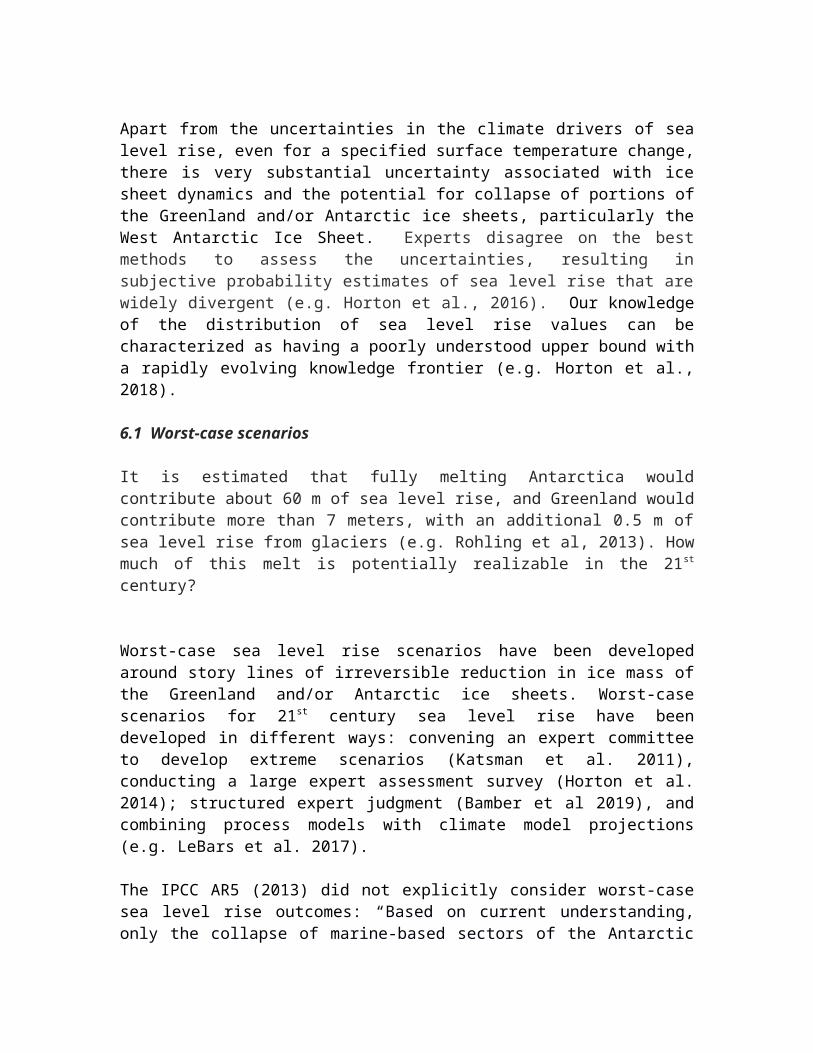
Apart from the uncertainties in the climate drivers of sea level rise, even for a specified surface temperature change, there is very substantial uncertainty associated with ice sheet dynamics and the potential for collapse of portions of the Greenland and/or Antarctic ice sheets, particularly the West Antarctic Ice Sheet. Experts disagree on the best methods to assess the uncertainties, resulting in subjective probability estimates of sea level rise that are widely divergent (e.g. Horton et al., 2016). Our knowledge of the distribution of sea level rise values can be characterized as having a poorly understood upper bound with a rapidly evolving knowledge frontier (e.g. Horton et al., 2018).

6.1 Worst-case scenarios

It is estimated that fully melting Antarctica would contribute about 60 m of sea level rise, and Greenland would contribute more than 7 meters, with an additional 0.5 m of sea level rise from glaciers (e.g. Rohling et al, 2013). How much of this melt is potentially realizable in the 21st century?

Worst-case sea level rise scenarios have been developed around story lines of irreversible reduction in ice mass of the Greenland and/or Antarctic ice sheets. Worst-case scenarios for 21st century sea level rise have been developed in different ways: convening an expert committee to develop extreme scenarios (Katsman et al. 2011), conducting a large expert assessment survey (Horton et al. 2014); structured expert judgment (Bamber et al 2019), and combining process models with climate model projections (e.g. LeBars et al. 2017).

The IPCC AR5 (2013) did not explicitly consider worst-case sea level rise outcomes: “Based on current understanding, only the collapse of marine-based sectors of the Antarctic ice sheet, if initiated, could cause global mean sea level to rise substantially above the likely range during the 21st century. This potential additional contribution cannot be precisely quantified but there is medium confidence that it would not exceed several tenths of a meter of sea level rise during the 21st century.”

Prior to the availability of sophisticated ice sheet model simulations, the rationale for the high-end scenarios of sea level rise was provided by geological evidence that related sea levels to global mean surface temperatures during current and previous interglacials (e.g. Rahmstorf, 2007). Jevrejeva et al. (2014) provides a summary of the worst-case (high-end) sea level rise scenarios by 2100, prior to the availability of projections from process-based ice sheet models:

Delta Commission in the Netherlands - 2008: 1.1 m Scientific Committee on Antarctic Research – 2009: 1.4 m United Kingdom Climate Impacts Programme - 2009: 1.9 m US Army Corps of Engineers - 2011: 1.5 m Arctic Monitoring and Assessment Programme - 2012: 1.6 m Third U.S. National Climate Assessment - 2012: 2 m

Since the IPCC AR5 and publication of Jevrejeva et al. (2014), substantial progress has been made in developing process-based models of ice sheets to predict 21st century sea level rise. Some of these studies have produced probability distributions of sea level rise, including a focus on the upper tail (e.g. Kopp et al. 2014; 2017). As discussed in Kopp et al. (2017) and Hinkel et al. (2019), upper bounds of future sea level rise projections remain deeply uncertain.

The worst-case (H++) sea level rise scenario for 2100 has been assessed by NOAA (2017) to be 2.5 m, which incorporated feedbacks related to marine ice-cliff instabilities (MICI) and ice-shelf hydrofracturing (DeConto and Pollard, 2016). DeConto and Pollard’s high-end estimate exceeded 1.7 m of sea level rise by 2100 from Antarctica alone.

The most recent assessment of high-end sea level rise by 2100 is reported by Bamber et al. (2019). Bamber et al. used structured expert judgment as the basis for developing a probability distribution of global sea level rise by 2050 and 2100 in response to 2 and 5 oC global temperature increase (Figure 3). The 2100 H refers to the scenario with 5 oC warming. The 95th percentile value value is 238 cm, which tracks the high end of published worst-case projections for 2100. While the 95th percentile value was the subject of explicit query of the experts, the 99 th percentile value of 329 cm was determined from

subjective assumptions about the shape of the probability distribution and is not associated with any obvious physical justification.

Figure 3. Global mean sea level rise projections from Bamber et al. (2019). L refers to a 2oC warming by 2100 and H refers to a 5oC warming by 2100.

Bamber et al. (2019) concluded that experts’ assessment of uncertainties in projections of the ice sheet contribution to SLR have grown since publication of the IPCC AR5, reflecting negative learning. Bamber et al. acknowledge that structural errors remain probable and may have a large impact on tails of the distribution. While acknowledging the subjective judgment used in formulation the distributions, they argue that this framework allows for these extreme possibilities to be considered.

The highest values of projected sea level rise depend critically on the marine ice cliff instability mechanism (MICI) of DeConto and Pollard (2016). While this instability is physically plausible, this chain of processes has so far not been observed in the Antarctic. Edwards et al. (2019) finds that improved constraints for the MICI result in lower estimates of 21st century sea level rise, and that the MICI is not required to reproduce sea-level changes due to Antarctic ice loss in the mid-Pliocene epoch or the last interglacial period. Edwards et al. found the 95th percentile of Antarctic ice loss by 2100 to be less than 43 cm for the RCP8.5. DeConto et al. (2018) updated their model with improved calibration of their model physical parameters, and found considerably lower ice loss from the Antarctic during the 21st century.

Attempts have been made to identify ‘upper bounds’ for 21st century sea level rise using top-down constraints based on paleo-records and kinematic constraints on ice sheet discharge. Pfeffer et al. (2008) concluded that “increases (in sea level by 2100) in excess of 2 meters are physically untenable” based on kinematic constraints in ice sheet discharge. However, Pfeffer et al.’s constraint may be invalidated if grounding lines of the West Antarctic ice sheet retreat from stabilizing sills with warming. Rohling et al. (2013) applied a geologic perspective, and concluded that a 21st century increase exceeding 1.8 or 2 m would be unprecedented during geological interglacials.

6.2 Possibility distribution

In context of the possibilistic approach, a useful way to stratify the current knowledge base about a range of 21st century sea level outcomes is a possibility diagram (e.g. Mauris 2011). In constructing such a possibility diagram, a critical judgment relates to the bounds of the borderline implausible region, whereby the upper bound reflects the plausible worst-case scenario and the lower bound reflects the possible worst-case scenario.

In assessing worst-case sea level rise possibilities, Hinkel et al. (2019) provide a useful categorization of confidence levels:

1. Medium confidence: The AR5 ‘likely’ range of scenarios. 2. Low confidence: Probability distributions of studies that have

used the expert judgment to estimate probabilities beyond the likely range. Going beyond the likely range through expert judgment yields lower confidence results.

3. Very low confidence: Probability distributions of studies based on DeConto and Pollard (2016) (incorporating the marine ice cliff instability). Very low confidence is assigned to these studies due to their results being conditional on a single and observationally poorly constrained line of evidence (i.e., a single ice sheet model), and the much lower projections from the most recent studies.

Returning to the criteria that were articulated in Section 3.2, the plausible worst-case scenario includes at most one borderline impossible assumption. Candidate scenarios for the plausible worst case include:

Process-based models using RCP8.5, but no inclusion of marine ice cliff instability: 1.12 m (UKCP, 2018; 95th percentile)

Process-based models including marine ice cliff instability, but not RCP8.5: 1.58 m (Kopp et al., 2017; 95th percentile)

With regards to the possible worst case, Hinkel et al. (2019) argues that if the component maxima are possible, then the sum of these should also be possible, unless there is an anticorrelation among them. However, the joint likelihood of outcomes derived from multiple very low probability parameters/events (even if uncorrelated) rapidly approaches zero. Further, top-down constraints may refute such extreme scenarios.

With these considerations in mind, candidate scenarios for possible worst case include: Recent assessments of the H++ scenario of 2.5 m, which include RCP8.5 and

worst case ice sheet instability processes (e.g. Kopp et al., 2014; NOAA, 2017) Process-based models including both RCP8.5 and marine ice cliff instability.

LeBars et al. (2017) included all worst-case parameters (RCP8.5 and DeConto and Pollard’s worst case values for the West Antarctic Ice Sheet) into projections of 21st century sea level rise and determined a worst-case (99 percentile) value of 3.39 cm for RCP8.5.

Kopp et al. (2017) employed a different analytical approach from LeBars et al. and determined a 99.9 percentile value of 2.97 cm

Geological constraints: 2 m (Rohling et al. 2013); exceedence would require conditions without natural interglacial precedents.

Pfeffer et al. (2008): 2 m from ice sheet kinematic constraints

Based on the above considerations, a possibility diagram is constructed. The variable U denotes the outcome for 21st century sea level change. U is cumulative, so that a higher outcome must necessarily first pass through lower values of sea level rise; values less than U therefore represent partial positions for U. Following the classification introduced in section 3.1, values of U are assigned the following values of π(U) (Figure 4):

π(U) ≥ 0.9: sea level rise up to 0.3 m; corroborated possibilities based on historical observations of rates of sea level rise (e.g. IPCC AR5)

0.5 > π(U) > 0.9: sea level rise exceeding 0.3 m and up to 0.63 m; verified possibilities contingent on T, based on IPCC AR5 likely range (but excluding RCP8.5).

0.5 ≥ π(U) > 0.1: sea level rise exceeding 0.63 m and up to 1.6 m; unverified possibilities contingent on the amount of predicted warming (from recent assessments, with at most one borderline implausible assumption)

0.1 ≥ π(U) > 0: sea level rise between 1.6 and 2.5 m; borderline implausible (including the possible worst cases and bordering the plausible worst case)

π(U) ≤ 0: sea level rise exceeding 2.5 m; impossible based upon background knowledge; refuted by observations or without physical justification; generated by pure speculation or statistically-manufactured fat tail

π(U) ≤ 0: negative values of sea level change; impossible based on background knowledge

The possibility diagram for sea level rise projections considers sea level rise outcomes as resulting from a cumulative process, whereby a higher sea level outcome must first pass through lower levels of sea level rise. Therefore, lower values of sea level rise represent partial positions for the higher scenario. Partial positions can discriminate between lower values for which we have greater confidence, versus higher values that are more speculative.

Figure 4 differs from the possibility diagram for 21st century sea level rise of LeCozannet et al. (2017), whereby the most probable value of sea level rise has the largest value. By contrast, in Figure 4 the IPCC ‘likely’ range of 0.3-0.63 m has lower values of than values < 0.3 m, even though values of 0.3-0.63 m are generally deemed to have a greater likelihood of representing the actual outcome of 21st century sea level rise. A sea level rise outcome of at least 0.2 m is by definition more likely than an outcome of at least 0.6 m; refutation of a sea level rise outcome of at least 0.6 m would not necessarily imply refutation of an outcome of at least 0.2 m. As also explained in section 5 on climate sensitivity, the values shown in Figure 4 are not inconsistent with the relative likelihoods (e.g. LeCozannet et al.); rather the values in Figure 4 reflect a different measure with different information content, focused on supporting partial positions and assessing the knowledge base for worst case scenarios.

Figure 4: Possibility diagram of projections of cumulative 21st century sea level rise.

The assignments in Figure 4 are based on justifications provided in the previous subsection (see also Curry, 2018b); however, this particular classification represents the judgment of one individual analyst (the author). One can envision an ensemble of curves, using different assumptions and judgments from different analysts. The point is not so much the exact numerical judgments provided here, but rather to demonstrate a way of stratifying the current knowledge base that is consistent with deep uncertainty, disagreement among experts and a rapidly evolving knowledge base.

The boundaries for the plausible/possible worst-case scenarios are expected to move with the knowledge frontier related to ice sheet instability processes. Further, these scenarios are contingent on the amount warming that is actually realized in the 21st century.

6.3 Alternative scenarios

All of the 21st century sea level rise scenarios are contingent on the amount of predicted warming. Additional scenarios of future warming or high frequency variability discussed in Section 3 may combine with manmade global warming to cross certain thresholds of ice sheet behavior sooner or later relative to what is expected from climate-model based projections driven by anthropogenic emissions/concentration scenarios.

Consider the following examples of known neglecteds related to 21st century sea level rise – processes that are at least somewhat understood and relevant on decadal to century timescales, but have been neglected owing to the focus on anthropogenic global warming.

Large-scale ocean circulation patterns having timescales from decadal to millennial not only influence local sea level rise, but also influence global sea level rise though their impacts on ice sheet mass balance. Fettweis et al. (2017), Mernild et al. (2017) and Hahn et al. (2018) have identified the dominant importance of the Atlantic Multidecadal Oscillation and North Atlantic Oscillation on the mass balance of the Greenland ice sheet. A related example is the influence of 20th century solar radiation variations on Greenland temperature and mass balance (Kobashi et al. 2015). Of relevance to the West Antarctic Ice Sheet, Jenkins et al. (2018) identified a cycle of warming and cooling in the Amundsen Sea, with ice sheet melt changing by a factor of 4 over decadal time scales, linked to El Niño events. On longer time scales, stochastic atmospheric forcing has been proposed as a cause of Greenland climate transitions on century time scales (Kleppin and Jochum, 2015). A reconstruction of West Antarctic surface mass balance since 1800 (Wang et al. 2019) found significant negative trend in West Antarctic ice sheet mass balance during the 19th century, but a positive trend between 1900 and 2010; clearly these trends are not driven by the same processes that produce global surface temperature trends. Bond et al. (1997) identified a pervasive millennial-scale cycle in the Northern Hemisphere climate that impacts the Greenland mass balance. Colgan et al. (2015) address the importance of millennial scale ice dynamics in the Greenland ice sheet mass balance. Changing oceanic conditions have been shown to be a fundamental contributor to ice sheet evolution on millennial time scales for the Greenland ice sheet (Tabone et al., 2018) and for the Antarctic ice sheet (Blasco et al. 2018).

In addition to the known unknowns associated with the marine ice shelf and ice cliff instabilities, there is a growing awareness of the importance of geological processes in the mass balance of the ice sheets (e.g. Whitehouse et al. 2019). In Greenland, newly discovered subglacial topographic features (Morlighem et al. 2017) reveal that many marine terminating glaciers are more exposed to warm subsurface Atlantic Water than previously thought. Alley et al. (2019) address millennial-scale tectonic oscillations in context of the stability of the Greenland Ice Sheet. In the West Antarctic, there is new evidence suggesting that sub-glacial meltwater production is influenced by an active volcanic geothermal heat source. De Vries et al. (2017) identified 138 volcanoes that are widely distributed throughout West Antarctic. Loose et al. (2018) identified an active volcanic heat source beneath the Pine Island Glacier, which is the fastest moving and fastest melting glacier in Antarctica. A recent paper by Barletta et al. (2018) found that the ground under the rapidly melting Amundsen Sea Embayment of West Antarctica is rising at the astonishingly rapid rate of 41 mm/yr, which is acting to stabilize the ice sheet (Gomez et al, 2015).

In summary, 21st century sea level rise projections driven solely by projected warming from anthropogenic emissions are arguably useful in assessing potential impacts from anthropogenic climate change. However, such projections neglect what may be important if not dominant process in the actual evolution of 21st century sea level rise, which is the relevant issue for adaptation decisions and local risk management. Neglecting known processes and failing to speculate about processes at the knowledge frontier increase the risk of a big surprise of either significantly more or less sea level rise in the 21 st century relative to current consensus projections, with several of these processes having

important implications for assessing worst-case scenarios. 7. Conclusions

The purpose of generating scenarios of future outcomes is that we should not be too surprised when the future eventually arrives. Projections of 21st century climate change and sea level rise are associated with deep uncertainty and rapidly advancing knowledge frontiers. The objective of this paper has been to articulate a strategy for portraying scientific understanding of the full range of possible scenarios of 21st century climate change and sea level rise in context of a rapidly expanding knowledge base, with a focus on worst-case scenarios.

A classification of future scenarios is presented, based on relative immunity to rejection relative to our current background knowledge and assessments of the knowledge frontier. The logic of partial positions allows for clarifying what we actually know with confidence, versus what is more speculative and uncertain or impossible. To avoid the Alice in Wonderland syndrome of scenarios that include too many implausible assumptions, published worst-case scenarios are assessed using the plausibility criterion of including only one borderline implausible assumption (where experts disagree on plausibility).

The possibilistic framework presented here provides a more nuanced way for articulating our foreknowledge than either by attempting, on the one hand, to construct probabilities of future outcomes, or on the other hand simply by labeling some statements about the future as possible. The possibilistic classification also avoids ignoring scenarios or classifying them as extremely unlikely if they are driven by processes that are poorly understood or not easily quantified.

The concepts of the possibility distribution, worst-case scenarios and partial positions are relevant to decision making under deep uncertainty (e.g. Walker et al. 2016), where precautionary and robust approaches are appropriate. Consideration of worst-case scenarios is an essential feature of precaution. A robust policy is defined as yielding outcomes that are deemed to be satisfactory across a wide range of plausible future outcomes. Robust policy making interfaces well with possibilistic approaches that generate a range of possible futures (e.g. Lempert et al. 2012). Partial positions are of relevance to flexible defense measures in the face of deep uncertainty in future projections (e.g. Oppenheimer and Alley, 2017).

Returning to Ackerman’s (2017) argument that policy should be based on the credible worst-case outcome, the issue then becomes how to judge what is ‘credible.’ It has been argued here that a useful criterion for a plausible (credible) worst-case climate outcome is that at most one borderline implausible assumption – defined as an assumption where experts disagree as to whether or not it is plausible – is included in developing the scenario. Using this criterion, the following summarizes my assessment of the plausible (credible) worst-case climate outcomes, based upon our current background knowledge:

The largest rates of warming that are often cited in impact assessment analyses (e.g. 4.5 or 5 oC) rely on climate models being driven by a borderline implausible

concentration/emission scenarios (RCP8.5). The IPCC AR5 (2013) likely range of warming at the end of the 21st century has a

top-range value of 3.1 oC, if the RCP8.5-derived values are eliminated. Even the more moderate amount of warming of 3.1oC relies on climate models with values of the equilibrium climate sensitivity that are larger than can be defended based on analysis of historical climate change. Further, these rates of warming explicitly assume that the climate of the 21st century will be driven solely by anthropogenic changes to the atmospheric concentration, neglecting 21st century variations in the sun and solar indirect effects, volcanic eruptions, and multi-decadal to millennial scale ocean oscillations. Natural processes have the potential to counteract or amplify the impacts of any manmade warming.

Estimates of 21st century sea level rise exceeding 1 m require at least one borderline implausible or very weakly justified assumption. Allowing for one borderline implausible assumption in the sea level rise projection produces estimates of sea level rise of 1.1 to 1.6 m. Higher estimates are produced using multiple borderline implausible or very weakly justified assumptions. The most extreme of the published worst-case scenarios require a cascade of events, each of which are extremely unlikely to borderline impossible based on our current knowledge base. However, given the substantial uncertainties and unknowns surrounding ice sheet dynamics, these scenarios should not be rejected as impossible.

The approach presented here is very different from the practice of the IPCC assessments and their focus on determining a likely range driven by human-caused warming. In climate science there has been a tension between the drive towards consensus to support policy making versus exploratory speculation and research that pushes forward the knowledge frontier (e.g. Curry and Webster, 2013). The possibility analysis presented here integrates both approaches by providing a useful framework for integrating expert speculation and model simulations with more firmly established theory and observations. This approach demonstrates a way of stratifying the current knowledge base that is consistent with deep uncertainty, disagreement among experts and a rapidly evolving knowledge base. Consideration of a more extensive range of future scenarios of climate outcomes can stimulate climate research as well as provide a better foundation for robust decision making under conditions of deep uncertainty.

References

Ackerman, F., 2017. Worst-Case Economics: Extreme Events in Climate and Finance. London: Anthem Press.

Alley RB, D Pollard, BR Parizek et al. (2019) Possible role for tectonics in the evolving stability of the Greenland Ice Sheet. J. Geophys. Res., 124, 97–115.

Annan, JD, JC Hargreaves (2006) Using multiple observationally-based constraints to estimate climate sensitivity. Geophys. Res. Lett, 33, L06704.

Aven T, O Renn (2015) An evaluation of the treatment of risk and uncertainties in the IPCC reports on climate change. Risk Analysis, 35, 701-712.

Bamber JL, and WP Aspinall (2013). An expert judgment assessment of future sea level rise from the ice sheets. Nature Clim. Change, 3, 424–427.

Bamber, JL et al. (2019) Ice sheet contributions to future sea level rise from structured expert judgment. PNAS, www.pnas.org/cgi/doi/10.1073/pnas.1817205116

Barletta, VR, M Bevis, BE Smith, et al. (2018) Observed rapid bedrock uplift in Amundsen Sea Embayment promotes ice-sheet stability. Science, 360, 1335-1339.

Betz G (2010) What’s the worst case? The methodology of possibilistic prediction. Analyse & Kritik, 01/2010, 87-106.

Blasco J, et al. (2019) The Antarctic Ice Sheet response to glacial millennial-scale variability. Clim. Past, 15, 121-133. Bond G, W Showers, M Cheseby, et al. (1997) A pervasive millennial-sale cycle in North Atlantic Holocene and glacial climates. Science, 278, 1257-1266.

Charney et al. (1979) Carbon Dioxide and Climate: A Scientific Assessment. National Academies of Science, DOI 10.17226/12181

Christensen, P et al. (2018) Uncertainty in forecasts of long-run economic growth. PNAS, 115, 5409-5414.

Colgan W, JE Box, ML Andersen, et al. (2015) Greenland high-elevation mass balance: inference and implication of reference period (1961-90) imbalance. Ann. Glaciol., 56, doi: 10.3189/2015AoG70A967

Curry, JA (2011a) Reasoning about climate uncertainty. Climatic Change, 108, 723-740.

Curry, JA (2011b) Nullifying the climate null hypothesis. WIRES Climate Change, 2, DOI: 10.1002/wcc.141 Curry, JA and PJ Webster (2013) Climate change: no consensus on consensus. CAB Reviews, 8, 1-9.

Curry, JA (2018a) Climate Uncertainty and Risk, CLIVAR Variations, 16, Number 3. https://indd.adobe.com/view/da3d0bde-1848-474d-b080-f07200293f9

Curry, J.A. (2018b) Sea Level Rise and Climate Change. CFAN Special Report, Climate Forecast Applications Network, 78 pp. https://docs.wixstatic.com/ugd/867d28_f535b847c8c749ad95f19cf28142256e.pdf

DeConto RM, D Pollard (2016) Contribution of Antarctica to past and future sea-level rise. Nature, 531, 591-597.

DeConto,RM, D Pollard, KA Christianson, RB Alley (2018) Climatic thresholds for widespread ice shelf hydrofracturing and ice cliff calving in Antarctica: implications for future sea level rise. American Geophysical Union, Fall Meeting 2018, abstract #GC13D-1046 http://adsabs.harvard.edu/abs/2018AGUFMGC13D1046D

De Vries VW, RG Bingham, AS Hein (2018) A new volcanic province: an inventory of subglacial volcanoes in West Antarctica. Geological Society, London, Special Publications, 461, 231.

DuBois D and H Prade (2011) Possibility theory and its applications: where do we stand? Springer Handbook of Computational Intelligence, pp 31-60

Edwards, TL, MA Brandon, G Durand et al. (2018) Revisiting Antarctic ice loss due to marine ice-cliff instability. Nature, 566, 58-64.

Eyring et al. (2019) Status of the Coupled Model Intercomparison Project Phase 6 (CMIP6) and Goals of the Workshop. CMI6 Analysis Workshop, Barcelona, Spain

Fettweis X, J Box, C Agosta, et al. (2017) Reconstructions of the 1900-2015 Greenland ice sheet mass balance using the regional climate MAR model. The Cryosphere, 11, 1015-2017.

Flage R and T Aven (2009) Expressing and communicating uncertainty in relation to quantitative risk analysis. Reliability & Risk Analysis: Theory & Applications, 2, 9–18.

Friedman N and JY Halpern, (1995) Plausibility measures: a user’s guide. In P. Besnard and S. Hanks (Eds.), Proc. Eleventh Conference on Uncertainty in Artificial Intelligence, pp. 175–184

Gettelman et al. (2019) High climate sensitivity in the Commuity Earth System Model Version 2 (CESM2). Geophys. Res. Lett, 46, 8329-8337.

Golledge, N. R., et al. (2019). Global environmental consequences of 21st century ice‐sheet melt. Nature, 566, 65–72.

Golaz et al. (2019) The DOE E3SM coupled model version 1: Overview and evaluation at standard resolution. J. Adv. In Modeling Earth Systems

Gomez N, D Pollard, D Holland (2015) Sea-level feedback lowers projections of future Antarctic ice sheet loss. Nature Comm., 6, 8798.

Hahn L, C Ummenhofer, YO Kwon (2018) North Atlantic natural variability modulates emergence of widespread Greenland melt in a warming climate. Geophys. Res. Lett, 45, 9171-

9178.

Hinkel, J et al. (2019). Meeting user needs for sea level rise information: A decision analysis perspective. Earth's Future, 7, 320–337.

Horton B, S Rahmstorf, SE Engelhart, AC Kemp (2014) Expert assessment of sea-level rise by AD 2100 and AD 2300. Quaternary Sci. Rev., 84, 1–6

Horton BP, S Rahmstorf, SE Engelhart, AC Kemp (2016) Reply to comment received from J.M. Gregory et al. regarding “Expert assessment of future sea-level rise by 2100 and 2300 AD”. Quaternary Sci. Rev., 97, 195-196

Horton BP, RE Kopp, AJ Garner, et al. (2018) Mapping sea-level change in time, space and probability. Ann. Rev. Environ. Resour., 43, 481-521.

Huber, F (2008) The plausibility-informativeness theory. In New waves in epistemology. Ed V. Hendricks, Palgrave Macmillin, pp 164-191.

IPCC AR4 (2007) Climate Change 2013: The Physical Science Basis. Contribution of Working Group I to the Fifth Assessment Report of the Intergovern- mental Panel on Climate Change [Solomon, S. et al. (eds.)]. Cambridge University Press, Cambridge, United Kingdom and New York, NY, USA, 1535 pp.

IPCC AR5 (2013) Climate Change 2013: The Physical Science Basis. Contribution of Working Group I to the Fifth Assessment Report of the Intergovernmental Panel on Climate Change [Stocker, T.F. et al. (eds.)]. Cambridge University Press, Cambridge, United Kingdom and New York, NY, USA, 1535 pp.

Jenkins A, D Shoosmith, P Dutrieux, et al. (2018) West Antarctic Ice Sheet retreat in the Amundsen Sea driven by decadal oceanic variability. Nature Geoscience, 2018; DOI: 10.1038/s41561-018-0207-4

Jevrejeva S., JC Moore, A Grinsted, A.Matthews, G Spada (2014) Trends and acceleration in global and regional sea levels since 1807. Global and Planetary Change, 113. 11-22. 

Katsman CA, A Sterl, JJ Beersma, et al. (2011) Exploring high-end scenarios for local sea level rise to develop flood protection strategies for a low-lying delta—the Netherlands as an example. Clim. Change, 109, 617-645.

Kleppin H, M Jochum (2015) Stochastic atmospheric forcing as a cause of Greenland climate transitions. J. Climate, 28, 7741-7763.

Knutson TR, JJ Sirutis, GA Vecchi et al. (2013) Dynamical downscaling projections of late 21st century Atlantic hurricane activity: CMIP3 and CMIP5 model-based scenarios. J. Climate, DOI: 10.1175/JCLI-D-12-00539.1

Knutti et al. (2017) Beyond equilibrium climate sensitivity. Nature Geoscience, DOI: 10.1030/NGEO3017

Kobashi T., JE Box, BM Vinther,et al. (2015), Modern solar maximum forced late twentieth century Greenland cooling, Geophys. Res. Lett., 42, 5992–5999, doi:10.1002/2015GL064764.

Kopp RE, RM Horton, CM Little, et al. (2014), Probabilistic 21st and 22nd century sea-level projections at a global network of tide-gauge sites, Earth’s Future, 2, 383–406.

Kopp RE, RM DeConto, D Bader, et al. (2017). Evolving Understanding of Antarctic Ice-Sheet Physics and Ambiguity in Probabilistic Sea-Level Projections, Earth’s Future, 5, 1217–1233

Kriegler E, N Bauer, A Popp et al. (2018) Fossil-fueled development (SSP5): An energy and resource intensive scenario for the 21st century. Global Environ. Change, 42, 297-315.

Kwakkel JH, W. E. Walker, and V. A. W. J. Marchau. 2010: Classifying and communicating uncertainties in model-based policy analysis. Int. J. Tech., Pol. Mgt, 10, 299–315.

LeBars D, S Drijfhout, H de Vries (2017) A high-end sea level rise probabilistic projection including rapid Antarctic ice sheet mass loss. Environ. Res. Lett., 12, doi:10.1088/1748-9326/aa6512.

LeCozannet G, JC Manceau, J Rohmer (2017) Bounding probabilistic sea-level projections within the framework of the possibility theory. Environ. Res. Lett., 12, 014012.

Lempert R, RL Sriver, K Keller (2012) Characterizing uncertain sea level rise projections to support investment decisions. California Energy Commission. Publication Number: CEC-500-2012-056.

Lewis, N, JA Curry (2015) The implications for climate sensitivity of AR5 forcing and heat uptake estimates. Climate Dynamics, 45, 1009-1023

Lewis, N., J.A. Curry (2018) The impact of recent forcing and ocean heat uptake data on estimates of climate sensitivity. J. Climate, https://doi.org/10.1175/JCLI-D-17-0667.1

Lewis, N and P Grunwald (2018) Objectively combining AR5 instrumental period and paleoclimate sensitivity evidence. Clim Dyn, DOI 10.1007/s00382-017-3744-4

Loose, B, AC Naveira Garabato, P Schlosser et al. (2018) Evidence of an active volcanic heat source beneath the Pine Island Glacier. Nature Comm., 9, Article # 2431.

Lukyanenko R. (2015) Falsification or confirmation: from logic to psychology. viXra, 1510, 1-7.

Mauris G (2011) Possibility distributions: A unified representation of direct-probability-based parameter estimation methods. Int. J. Approx. Reasoning, 52, 1232-1242.

Mauritsen et al. (2019) Developments in the MPI-M Earth System Model version 1.2 (MPI-ESM1.2) and its response to increasing CO2. J. Adv. In Modeling Earth Systems.

Mernild SH, GE Liston, AP Beckerman, JC Yde (2017) Reconstruction of the Greenland Ice Sheet surface mass balance and the spatiotemporal distribution of freshwater ruoff from Greenland to surrounding seas. The Cryosphere, https://doi.org/10.5194/tc-2017-234

Morlighem M, CN Williams, E Rignot, et al.. (2017). BedMachine v3: Completebed topography and ocean bathymetry mapping of Greenland from multibeam echo sounding combined with mass conservation. Geophys. Res. Lett., 44, 11,051–11,061.

NAS (2018) Learning from the Science of Cognition and Perception for Decision Making: Proceedings of a Workshop. National Academies Press DOI 10.17226/25118

NOAA (2017) Global and regional sea level rise scenarios for the United States. NOAA Technical Report NOS CO-OPS 083.

O’Neill BC, C Tebaldi, DP van Vuuren et al. (2016) The Scenario Model Intercomparison Project (ScenarioMIP) for CMIP6. Geosci. Model Dev., 9, 3461–3482

Oppenheimer M, BC O’Neill, M Webster, S Agrawala (2007) The Limits of Consensus, Science, 317, 1505-1506.

Oppenheimer et al. (2008) Negative learning. Climatic Change, 89. 155-172.

Oppenheimer M, CM Little, RM Cooke (2016) Expert judgment and uncertainty quantification for climate change. Nature Clim. Change, 6, DOI: 10.1038/NCLIMATE2959

Oppenheimer, M and RB Alley (2017) How high will the seas rise? Science, 345, 1375.

Parker WS, JS Risbey (2015) False precision, surprise and improved uncertainty assessment. Phil. Trans A, 373, 2014053.

Pfeffer WT, JT Harper, S O’Neal (2008) Kinematic constraints on glacier contributions to 21st-century sea-level rise. Science, 321, 1340-1343.

Rahmstorf S (2007) A semi-empirical approach to projecting future sea-level rise. Science, 315, 368.

Riahi K, Rao S, Krey V, et al. (2011) RCP 8.5da scenario of comparatively high greenhouse gas emissions. Clim. Change, 109: 33e57.

Riahi K, DP van Vuuren, E Kriegler et al. (2017) The Shared Socioeconomic Pathways and their energy, land use, and greenhouse gas emissions implications: An overview. Global Environ. Change, 42, 153-168

Ritchie J, H Dowlatabadi (2017) Why do climate change scenarios return to coal? Energy, 140, 1276-1291.

Rohling, EJ, et al. (2013) A geological perspective on future sea level rise. Scientific Reports, 3, 3461 DOI: 10.1038/srep03461

Samir KC and W Lutz (2014) The human core of the shared socioeconomic pathways: population scenarios by age, sex and level of education for all countries to 2100. Global Environmental Change, 42, 181-192

Shackle DLS (1961) Decision, Order and Time in Human Affairs, 2nd edition, Cam- bridge University Press, UK.

Shepherd TG, E Boyd, RA Calel et al. (2018) Storylines: an alternative approach to representing uncertainty in physical aspects of climate change. Clim. Change, 151, 555-571.

Smith LA, N Stern (2011) Uncertainty in science and its role in climate policy. Phil. Trans. R. Soc. A, 369, 4818–4841.

Stainforth DA, MR Allen, ER Tredger, LA Smith, 2007: Confidence, uncertainty, and decision-support relevance in climate prediction. Phil. Trans. Roy. Soc. A, 365, 2145–2161, doi:10.1098/rsta.2007.2074.

Stevens, B., S. C. Sherwood, S. Bony, and M. J. Webb (2016), Prospects for narrowing bounds on Earth’s equilibrium climate sensitivity, Earth’s Future, 4, 512–522.Tabone I, A Robinson, J Alvarez-Solas, M Montoya (2019) Impact of millennial-scale oceanic variability on the Greenland ice-sheet evolution throughout the last glacial period. Clim. Past, 15, 593-609.

Trutnevyte E, C Guivarch, R Lempert, N Strachan (2016) Reinvigorating the scenario technique to expand uncertainty consideration. Clim. Change, 135, 373-379.

van Vuuren DP, J Edmonds, M Kainuma, et al (2011) The representative concentration pathways: an overview. Clim. Change, 109, 5-31.

UKCP (2018) UKCP18 Marine Report. Met Office Hadley Centre, 133 pp.

Voosen, P (2019) New climate models forecast a warming surge. Science, 364, 222-223.

Walker WE, RJ Lempert, JH Kwakkel, 2016: Deep Uncertainty. Encyclopedia of Operations Research and Management Science. Eds: SI Gass and MC Fu, Springer.

Wallace-Wells, D (2019) The Uninhabitable Earth: Life After Warming. Tim Duggan Books, 320 pp.

Wang J, L Feng, X Tang et al (2017) The implications of fossil fuel supply constraints on climate change projections – a supply side analysis. Futures, 86, 58-72.

Wang Y, B Huai, ER Thomas, MR van den Broek et al (2019) A new 200-year spatial reconstruction of West Antarctic surface mass balance. J. Geophys. Res, https://doi.org/10.1029/2018JD029601

Weitzman, ML (2009) On Modeling and Interpreting the Economics of Catastrophic Climate Change. Rev. Econ. Stat., 91, 1-19.

Whitehouse et al. (2019) Solid Earth change and the evolution of the Antarctic Ice Sheet. Nature Comm, https://doi.org/10.1038/s41467-018-08068-y