Introduction · We present e cient algorithms for solving Legendre equations over Q(equivalently,...

MATHEMATICS OF COMPUTATIONVolume 72, Number 243, Pages 1417–1441S 0025-5718(02)01480-1Article electronically published on December 18, 2002

EFFICIENT SOLUTION OF RATIONAL CONICS

J. E. CREMONA AND D. RUSIN

Abstract. We present efficient algorithms for solving Legendre equations overQ (equivalently, for finding rational points on rational conics) and parametriz-ing all solutions. Unlike existing algorithms, no integer factorization is re-quired, provided that the prime factors of the discriminant are known.

1. Introduction

1.1. Summary of results. In this paper we give efficient methods of finding allrational points on a rational conic C given by a nonsingular homogeneous equationof degree 2:

(1) C : f(X,Y, Z) = 0.

One method for finding one rational point on C, if one exists, is the originaldescent method of Legendre. We show how one may easily make a significantimprovement to this (reducing the number of iterations from exponential in thesize of the input to linear); and also, but with more work, make an even greaterimprovement. This last method involves no integer factorization other than thatof the discriminant of the original equation (which is in any case necessary fordeciding the solubility of (1)). It is the necessity of factoring “spurious” integersarising during the course of the computation which is the bottleneck in simplerreduction methods; our “factorization-free” method avoids this entirely.

We also describe a factorization-free method of solution based on lattice reduc-tion; this is not original, though apparently not well known.

We present examples and timings of our implementation of both methods; theseindicate that the reduction method is faster in practice than the lattice-basedmethod. Both are linear time, given a so-called solubility certificate (defined below),and probabilistic polynomial time given only the factorization of the discriminant.

As an example of the speed which is now attainable, the solution of an equationof the form ax2 + by2 = cz2, where a, b and c are 200-digit primes, takes less than2 seconds on a modest PC. Such a problem is not feasible to solve in reasonabletime with Legendre’s method (as in Maple, for example).

We also show how to parametrize all rational points on C, given one point, in themost efficient way. This is necessary for several applications, such as to 2-descenton elliptic curves, and is also used for finding a small single solution to (1).

Received by the editor September 5, 2001.2000 Mathematics Subject Classification. Primary 11G30, 11D41.

c©2002 American Mathematical Society

1417

License or copyright restrictions may apply to redistribution; see http://www.ams.org/journal-terms-of-use

1418 J. E. CREMONA AND D. RUSIN

It would be useful and interesting to extend the algorithms presented here tonumber fields. We say little more about this here, but refer to the paper [11] byPohst, and Simon’s thesis [14].

The factorization-free algorithm presented here has been implemented in release2.8 (July 2001) of the package Magma.

1.2. Background. By the Hasse or local-global principle for curves of genus 0, thecurve C has rational points if and only if it has points everywhere locally. Thus,testing (1) for solubility is easy, at least in theory, and in practice no harder thanfactoring the discriminant of the given equation (see Section 2.2 below for details).

Our first main concern will be to find one solution efficiently when solutions exist.Here and throughout we will pass freely between the geometric language of “pointson curves” and the Diophantine language of “solutions to equations”. We alwaysexclude the trivial solution (x, y, z) = (0, 0, 0), as we are really interested in projec-tive solutions (x : y : z) ∈ P2(Q), each of which has a “primitive” representationwith x, y, z ∈ Z and gcd(x, y, z) = 1, unique up to sign.

Secondly, we will want to find a “small” solution. Holzer’s theorem (see below fora precise statement) asserts that a soluble equation always has solutions which arenot too large in terms of the coefficients. Any given solution may be reduced, usinga method of Mordell, until it satisfies Holzer’s bounds. We present an alternativereduction method, faster than Mordell’s, though the solution it gives may not bequite Holzer-reduced.

Finally, given one solution P0 = (x0, y0, z0) to (1), one can write down a para-metrization of all solutions of the form

(2) X = Q1(U, V ), Y = Q2(U, V ), Z = Q3(U, V ),

where eachQi(U, V ) ∈ Z[U, V ] is a quadratic form. Geometrically, the homogeneouscoordinates (U : V ) parametrize the pencil of lines through P0, each of whichintersects the conic C in a unique second point. Our final task will be to findsuch a parametric solution which is as simple as possible. We will see that aparametrization exists such that the discriminants of the polynomials Qi(U, V )are prescribed in terms of the coefficients of the defining polynomial f(X,Y, Z),independently of the particular basic solution P0 found earlier. This last point isparticularly significant in certain applications.

Our approach throughout will be algorithmic, and our results will be in the formof efficient algorithms to carry out the tasks we have just outlined. We will giveexamples to show that our method is more efficient, and leads to better (meaningsmaller) solutions than those which can be found elsewhere (for example, by usingthe Maple computer algebra system). The mathematics here is entirely elementary,and mostly also quite well-known, but we are not aware of a systematic treatmentof such equations in the literature which is both algorithmic and concerned withthe size of the parametric solutions obtained.

A slightly different problem is to parametrize all “primitive” integer solutions(x, y, z) to (1) using integer quadratics Qi(U, V ). Mordell showed that this is pos-sible using a finite family of quadratic parametrizations of the form (2). Since weare interested in projective solutions, we are not interested in the primitivity, andour task is therefore slightly simpler.

The application which led us to develop these methods is in higher descents onelliptic curves overQ, starting with a descent via 2-isogeny. See [5] for details of this.


EFFICIENT SOLUTION OF RATIONAL CONICS 1419

Another application of which we are aware is the determination of explicit equationsfor hyperelliptic curves whose Jacobians are quotients of modular Jacobians: seethe theses of Wilson [19] (Oxford, 1998) and Weber [17] (Essen, 1996) for examplesof these. It is remarkable that an algorithmic solution to the problem of findingall rational points on a curve of genus 0 has not yet been perfected (as remarkedby Mazur in [9]), given the current activity on a wide scale concerning constructivesolutions to Diophantine equations of higher genus, so it is interesting to note thatefficient solutions to this simpler problem are also required for the study of curvesof higher genus.

We are grateful to Denis Simon for the reference [12].

2. Single solutions

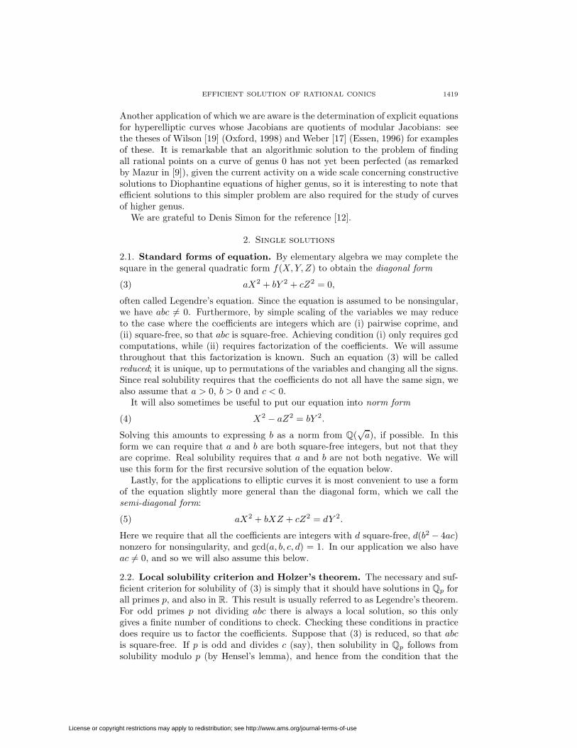
2.1. Standard forms of equation. By elementary algebra we may complete thesquare in the general quadratic form f(X,Y, Z) to obtain the diagonal form

(3) aX2 + bY 2 + cZ2 = 0,

often called Legendre’s equation. Since the equation is assumed to be nonsingular,we have abc 6= 0. Furthermore, by simple scaling of the variables we may reduceto the case where the coefficients are integers which are (i) pairwise coprime, and(ii) square-free, so that abc is square-free. Achieving condition (i) only requires gcdcomputations, while (ii) requires factorization of the coefficients. We will assumethroughout that this factorization is known. Such an equation (3) will be calledreduced; it is unique, up to permutations of the variables and changing all the signs.Since real solubility requires that the coefficients do not all have the same sign, wealso assume that a > 0, b > 0 and c < 0.

It will also sometimes be useful to put our equation into norm form

(4) X2 − aZ2 = bY 2.

Solving this amounts to expressing b as a norm from Q(√a), if possible. In this

form we can require that a and b are both square-free integers, but not that theyare coprime. Real solubility requires that a and b are not both negative. We willuse this form for the first recursive solution of the equation below.

Lastly, for the applications to elliptic curves it is most convenient to use a formof the equation slightly more general than the diagonal form, which we call thesemi-diagonal form:

(5) aX2 + bXZ + cZ2 = dY 2.

Here we require that all the coefficients are integers with d square-free, d(b2 − 4ac)nonzero for nonsingularity, and gcd(a, b, c, d) = 1. In our application we also haveac 6= 0, and so we will also assume this below.

2.2. Local solubility criterion and Holzer’s theorem. The necessary and suf-ficient criterion for solubility of (3) is simply that it should have solutions in Qp forall primes p, and also in R. This result is usually referred to as Legendre’s theorem.For odd primes p not dividing abc there is always a local solution, so this onlygives a finite number of conditions to check. Checking these conditions in practicedoes require us to factor the coefficients. Suppose that (3) is reduced, so that abcis square-free. If p is odd and divides c (say), then solubility in Qp follows fromsolubility modulo p (by Hensel’s lemma), and hence from the condition that the



Legendre symbol(−abp

)is +1. Hence the local conditions for all odd finite primes

are equivalent to the existence of solutions to the following quadratic congruences:

(6) X21 ≡ −bc (mod a); X2

2 ≡ −ca (mod b); X23 ≡ −ab (mod c).

Moreover, the number of local conditions which fail must be even (by the productformula for the Hilbert symbol), so the solubility of these congruences togetherwith the sign condition ensuring real solubility is already sufficient to ensure globalsolubility, and a 2-adic condition is not needed.

Definition 2.1. A triple (k1, k2, k3) ∈ Z3 is called a solubility certificate for (3) ifit gives a solution to the congruences (6).

We summarize the local solubility criterion as follows.

Lemma 2.1. Let a, b and c be nonzero integers with abc square-free, not all of thesame sign. Then (3) has a solution if and only if a solubility certificate exists.

If a, b and c are pairwise coprime (but not necessarily square-free), then theexistence of a solubility certificate is sufficient, but no longer necessary, for theexistence of solutions to (3).

A proof of the last statement is implicit in the algorithms below, which guaranteeto deliver a solution from a solubility certificate provided only that a, b and c arepairwise coprime and not all of the same sign. That the existence of the certificateis not necessary when the coefficients are square-free may be seen from the equation9X2 − Y 2 − Z2 = 0, which has the solution (1, 3, 0), but no certificate since thecongruence X2

1 ≡ −1 (mod 9) has no solution.To the triple of coefficients (a, b, c) and the certificate (k1, k2, k3) we will associate

a 3-dimensional sublattice L = L(a, b, c; k1, k2, k3) of Z3, called the solution latticefor the certificate, as follows:

L(a, b, c; k1, k2, k3) = {(x, y, z) ∈ Z3 |by ≡ k1z (mod a),

cz ≡ k2x (mod b),(7)

ax ≡ k3y (mod c)}.

The index of L(a, b, c; k1, k2, k3) in Z3 is |abc|. One easily checks that for (x, y, z) ∈L, we have ax2 + by2 + cz2 ≡ 0 (mod abc). In the second and third algorithms wepresent below, we will construct a solution of (3) which lies in the solution latticefor any given solubility certificate.

The first algorithm we give below for solving conics itself constitutes a proof ofLegendre’s theorem, since it is guaranteed to find a solution unless either a quadraticcongruence fails to be soluble, or the signs of the coefficients are wrong. Indeed,Legendre’s own proof follows the same lines: see the account in Weil’s historicalbook [18, p. 100]. Algorithmic solutions in the literature often follow essentially thesame reduction procedure as Legendre (see [8], or [15] for a recent example). As wewill see, this method has two disadvantages in practice: it takes many steps, each ofwhich involves the factorization of an integer, and the resulting solution can be verylarge. Our first improvement already performs better in these respects; although itdoes not eliminate the factorization from each step, the number of steps is reduced,the numbers to be factored are smaller, and the resulting solution is also smaller.Then the “factorization-free” version of the reduction method eliminates the needfor any factorization, given a solubility certificate, giving even greater improvement



and making possible the solution of equations whose coefficients have hundreds ofdigits in only a few seconds.

In the famous paper [1], in which higher descents were used to study the ranks ofelliptic curves of the form Y 2 = X3 −DX , the authors remark [1, p. 100] that thesolution of various auxiliary conics is the most time-consuming part of the descentprocess. We also found this to be true (despite having 30 years of factorizationtechnology to hand) before using the new methods described here.

Now assume that (3) is soluble. Holzer’s theorem asserts that there exists anintegral solution (x, y, z) with

(8) |x| ≤√|bc|, |y| ≤

√|ac|, |z| ≤

√|ab|,

or equivalently,

(9) max(|a|x2, |b|y2, |c|z2) ≤ |abc|.Such a solution we will call “Holzer-reduced”. Holzer’s theorem is not trivial toprove: see [3] for a recent fairly short proof, improving earlier versions by Mordelland Cassels (see section 2.4 below for more on this). In Mordell’s proof, one obtainsa solution which does not necessarily satisfy Holzer’s bounds, and then reduces thesolution using the following lemma from [10, Theorem 5, p. 47].

Lemma 2.2. Let a, b and c be nonzero integers with abc square-free, a > 0, b > 0and c < 0, and let (x0, y0, z0) be a solution of (3). If |z0| >

√ab, then there exists

a solution (x1, y1, z1) with |z1| < |z0|.

We will give Mordell’s construction below. After a finite number of steps, wearrive at a solution (x, y, z) with |z| ≤

√ab, and then the inequalities on x and y

follow immediately. We will also present a new method of reducing solutions whichis faster than Mordell’s, but only produces a solution satisfying

(10) max(|a|x2, |b|y2, |c|z2) ≤ 43|abc|.

A similar result concerning small solutions to Legendre’s equation over totallyreal number fields can be found in [11].

2.3. Algorithm I: Legendre-type reduction. The first algorithm for findingone solution works with the equation in the norm form (4), where the coefficientsa and b are square-free nonzero integers, not necessarily coprime. By symmetrywe may assume that |a| ≤ |b|, interchanging a and b if necessary. The idea, whichoriginates with Legendre, is to proceed by descent, reducing the problem of solving(4) to that of solving a similar equation with a smaller b coefficient. This step isrepeated until |b| < |a|, after which a and b are interchanged. The base cases inwhich no further descent is necessary are trivially dealt with. The full procedure isas follows.

Algorithm I.(1) If |a| > |b| then swap a and b, solve the resulting equation, then swap y

and z in the solution obtained.(2) If b = 1 then set (x, y, z) = (1, 1, 0) and stop.(3) If a = 1 then set (x, y, z) = (1, 0, 1) and stop.(4) If b = −1 there is no solution (since a must be −1).(5) If b = −a then set (x, y, z) = (0, 1, 1) and stop.



(6) If b = a then let (x1, y1, z1) be a solution of X21 +Z2

1 = aY 21 , set (x, y, z) =

(ay1, x1, z1) and stop.(7) Let w be a solution to X2 ≡ a (mod b) with |w| ≤ |b|/2, and set (x0, z0) =

(w, 1), so that x20 − az2

0 ≡ 0 (mod b).(8) Use lattice reduction to find a new nontrivial solution (x0, z0) to the con-

gruence X2 − aZ2 ≡ 0 (mod b), with x20 + |a|z2

0 as small as possible.(9) Set t = (x2

0 − az20)/b, and write t = t1t

22 with t1 square-free.

(10) Let (x1, y1, z1) be a solution to X2 − aZ2 = t1Y2; then

(x, y, z) = (x0x1 + az0z1, t1t2y1, z0x1 + x0z1)

is a solution to (4): stop.

By the end of step 6 we have reduced the problem to solving equations in which|b| ≥ 2, |b| > |a| and a 6= 1 (though a = −1 is possible). The reduction stepproceeds by first solving the quadratic congruence

X2 ≡ a (mod b)

to obtain a solution w with |w| ≤ |b|/2. The usual algorithm for this step involvesfactoring b, finding a square root of a modulo each prime divisor of b, and combiningthem with the Chinese Remainder Theorem. All these square roots must exist ifthe equation passes the local solubility criterion. We then have w2 − a = bt, wherethe integer t satisfies

|t| < 14|b|+ 1 ≤ 1

2|b|;

(here we use 1 ≤ |a| < |b|). The standard algorithm found in the literature (asin [15], for example) omits step 8, using the fact that this value of t is strictlyless than b to obtain a descent. This procedure works perfectly well in practice,provided that the initial coefficients a and b are fairly small. The size of the largercoefficient is reduced by a factor of approximately 4 at each step; the main problemwith large examples is the need to factor all the coefficients b which arise, in orderto solve the associated quadratic congruences.

Our improvement consists of inserting the extra step 8 above. We have onesolution (x0, z0) = (w, 1) to the congruence

(11) X2 − aZ2 ≡ 0 (mod b).

Using an elementary lattice reduction technique, we find the solution (x0, z0) to thiscongruence which minimizes x2 + |a|z2, and set t = (x2

0 − az20)/b. This will be very

much smaller than the earlier value of t. Explicitly, the minimal vector has lengthO(b√a), so we see that in Step 9, t will be O(

√a). Thus while the unimproved

method only reduces the size of ab (measured in bits, say) at a rate linear in thenumber of steps, in the improved method the size is reduced quadratically. Oneexpects that the number of digits in ab should be roughly halved with each iteration.We give an example in the next section.



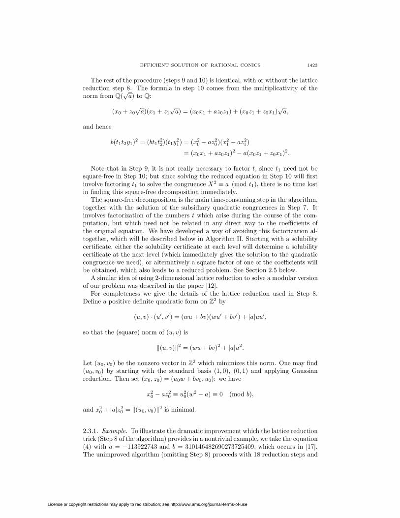
The rest of the procedure (steps 9 and 10) is identical, with or without the latticereduction step 8. The formula in step 10 comes from the multiplicativity of thenorm from Q(

√a) to Q:

(x0 + z0

√a)(x1 + z1

√a) = (x0x1 + az0z1) + (x0z1 + z0x1)

√a,

and hence

b(t1t2y1)2 = (bt1t22)(t1y21) = (x2

0 − az20)(x2

1 − az21)

= (x0x1 + az0z1)2 − a(x0z1 + z0x1)2.

Note that in Step 9, it is not really necessary to factor t, since t1 need not besquare-free in Step 10; but since solving the reduced equation in Step 10 will firstinvolve factoring t1 to solve the congruence X2 ≡ a (mod t1), there is no time lostin finding this square-free decomposition immediately.

The square-free decomposition is the main time-consuming step in the algorithm,together with the solution of the subsidiary quadratic congruences in Step 7. Itinvolves factorization of the numbers t which arise during the course of the com-putation, but which need not be related in any direct way to the coefficients ofthe original equation. We have developed a way of avoiding this factorization al-together, which will be described below in Algorithm II. Starting with a solubilitycertificate, either the solubility certificate at each level will determine a solubilitycertificate at the next level (which immediately gives the solution to the quadraticcongruence we need), or alternatively a square factor of one of the coefficients willbe obtained, which also leads to a reduced problem. See Section 2.5 below.

A similar idea of using 2-dimensional lattice reduction to solve a modular versionof our problem was described in the paper [12].

For completeness we give the details of the lattice reduction used in Step 8.Define a positive definite quadratic form on Z2 by

(u, v) · (u′, v′) = (wu + bv)(wu′ + bv′) + |a|uu′,

so that the (square) norm of (u, v) is

‖(u, v)‖2 = (wu + bv)2 + |a|u2.

Let (u0, v0) be the nonzero vector in Z2 which minimizes this norm. One may find(u0, v0) by starting with the standard basis (1, 0), (0, 1) and applying Gaussianreduction. Then set (x0, z0) = (u0w + bv0, u0): we have

x20 − az2

0 ≡ u20(w2 − a) ≡ 0 (mod b),

and x20 + |a|z2

0 = ‖(u0, v0)‖2 is minimal.

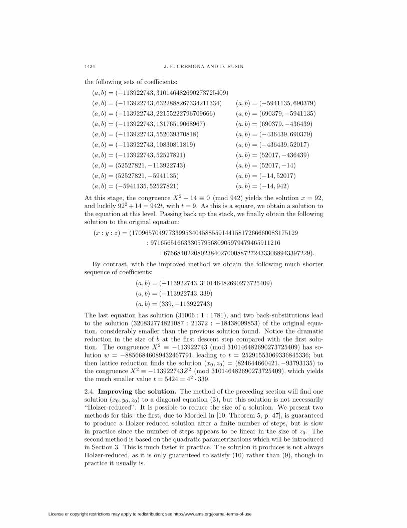
2.3.1. Example. To illustrate the dramatic improvement which the lattice reductiontrick (Step 8 of the algorithm) provides in a nontrivial example, we take the equation(4) with a = −113922743 and b = 310146482690273725409, which occurs in [17].The unimproved algorithm (omitting Step 8) proceeds with 18 reduction steps and



the following sets of coefficients:

(a, b) = (−113922743, 310146482690273725409)

(a, b) = (−113922743, 6322888267334211334) (a, b) = (−5941135, 690379)

(a, b) = (−113922743, 22155222796709666) (a, b) = (690379,−5941135)

(a, b) = (−113922743, 13176519068967) (a, b) = (690379,−436439)

(a, b) = (−113922743, 552039370818) (a, b) = (−436439, 690379)

(a, b) = (−113922743, 10830811819) (a, b) = (−436439, 52017)

(a, b) = (−113922743, 52527821) (a, b) = (52017,−436439)

(a, b) = (52527821,−113922743) (a, b) = (52017,−14)

(a, b) = (52527821,−5941135) (a, b) = (−14, 52017)

(a, b) = (−5941135, 52527821) (a, b) = (−14, 942)

At this stage, the congruence X2 + 14 ≡ 0 (mod 942) yields the solution x = 92,and luckily 922 + 14 = 942t, with t = 9. As this is a square, we obtain a solution tothe equation at this level. Passing back up the stack, we finally obtain the followingsolution to the original equation:

(x : y : z) = (17096570497733995340458855914415817266660083175129: 971656516633305795680905979479465911216

: 67668402208023840270008872724333068943397229).

By contrast, with the improved method we obtain the following much shortersequence of coefficients:

(a, b) = (−113922743, 310146482690273725409)

(a, b) = (−113922743, 339)

(a, b) = (339,−113922743)

The last equation has solution (31006 : 1 : 1781), and two back-substitutions leadto the solution (320832774821087 : 21372 : −18438099853) of the original equa-tion, considerably smaller than the previous solution found. Notice the dramaticreduction in the size of b at the first descent step compared with the first solu-tion. The congruence X2 ≡ −113922743 (mod 310146482690273725409) has so-lution w = −88566846089432467791, leading to t = 25291553069336845336; butthen lattice reduction finds the solution (x0, z0) = (824644660421,−93793135) tothe congruence X2 ≡ −113922743Z2 (mod 310146482690273725409), which yieldsthe much smaller value t = 5424 = 42 · 339.

2.4. Improving the solution. The method of the preceding section will find onesolution (x0, y0, z0) to a diagonal equation (3), but this solution is not necessarily“Holzer-reduced”. It is possible to reduce the size of a solution. We present twomethods for this: the first, due to Mordell in [10, Theorem 5, p. 47], is guaranteedto produce a Holzer-reduced solution after a finite number of steps, but is slowin practice since the number of steps appears to be linear in the size of z0. Thesecond method is based on the quadratic parametrizations which will be introducedin Section 3. This is much faster in practice. The solution it produces is not alwaysHolzer-reduced, as it is only guaranteed to satisfy (10) rather than (9), though inpractice it usually is.



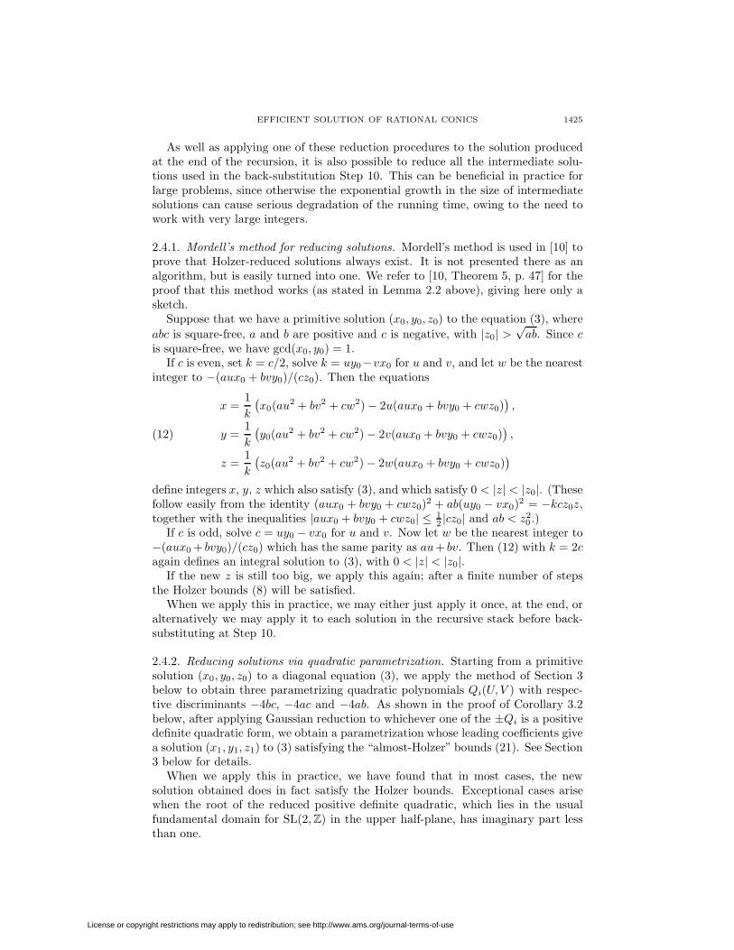
As well as applying one of these reduction procedures to the solution producedat the end of the recursion, it is also possible to reduce all the intermediate solu-tions used in the back-substitution Step 10. This can be beneficial in practice forlarge problems, since otherwise the exponential growth in the size of intermediatesolutions can cause serious degradation of the running time, owing to the need towork with very large integers.

2.4.1. Mordell’s method for reducing solutions. Mordell’s method is used in [10] toprove that Holzer-reduced solutions always exist. It is not presented there as analgorithm, but is easily turned into one. We refer to [10, Theorem 5, p. 47] for theproof that this method works (as stated in Lemma 2.2 above), giving here only asketch.

Suppose that we have a primitive solution (x0, y0, z0) to the equation (3), whereabc is square-free, a and b are positive and c is negative, with |z0| >

√ab. Since c

is square-free, we have gcd(x0, y0) = 1.If c is even, set k = c/2, solve k = uy0−vx0 for u and v, and let w be the nearest

integer to −(aux0 + bvy0)/(cz0). Then the equations

x =1k

(x0(au2 + bv2 + cw2)− 2u(aux0 + bvy0 + cwz0)

),

y =1k

(y0(au2 + bv2 + cw2)− 2v(aux0 + bvy0 + cwz0)

),(12)

z =1k

(z0(au2 + bv2 + cw2)− 2w(aux0 + bvy0 + cwz0)

)define integers x, y, z which also satisfy (3), and which satisfy 0 < |z| < |z0|. (Thesefollow easily from the identity (aux0 + bvy0 + cwz0)2 + ab(uy0 − vx0)2 = −kcz0z,together with the inequalities |aux0 + bvy0 + cwz0| ≤ 1

2 |cz0| and ab < z20 .)

If c is odd, solve c = uy0 − vx0 for u and v. Now let w be the nearest integer to−(aux0 + bvy0)/(cz0) which has the same parity as au+ bv. Then (12) with k = 2cagain defines an integral solution to (3), with 0 < |z| < |z0|.

If the new z is still too big, we apply this again; after a finite number of stepsthe Holzer bounds (8) will be satisfied.

When we apply this in practice, we may either just apply it once, at the end, oralternatively we may apply it to each solution in the recursive stack before back-substituting at Step 10.

2.4.2. Reducing solutions via quadratic parametrization. Starting from a primitivesolution (x0, y0, z0) to a diagonal equation (3), we apply the method of Section 3below to obtain three parametrizing quadratic polynomials Qi(U, V ) with respec-tive discriminants −4bc, −4ac and −4ab. As shown in the proof of Corollary 3.2below, after applying Gaussian reduction to whichever one of the ±Qi is a positivedefinite quadratic form, we obtain a parametrization whose leading coefficients givea solution (x1, y1, z1) to (3) satisfying the “almost-Holzer” bounds (21). See Section3 below for details.

When we apply this in practice, we have found that in most cases, the newsolution obtained does in fact satisfy the Holzer bounds. Exceptional cases arisewhen the root of the reduced positive definite quadratic, which lies in the usualfundamental domain for SL(2,Z) in the upper half-plane, has imaginary part lessthan one.



For example, the equation X2 + 3Y 2 = 91Z2 has the solution (19, 1, 2), whichis not Holzer-reduced since x2 = 361 > 273 = 3 · 91 and z2 = 4 > 3 = 1 · 3. Theparametrizing quadratics are X = 19U2 − 16UV − 11V 2, Y = U2 − 20UV + 9V 2

and Z = 2(U2 − UV + V 2), with minimal discriminants 1092 = −4 · 3 · (−91),364 = −4 · 1 · (−91) and −12 = −4 · 1 · 3 respectively. The latter is positivedefinite and reduced, with root (−1 + i

√3)/2, and this method cannot reduce the

solution further. However, applying Holzer’s method once to (19, 1, 2) gives theHolzer-reduced solution (4, 5, 1). The corresponding parametrizing quadratics areX = 4U2 + 30UV − 12V 2, Y = 5U2 − 8UV − 15V 2 and Z = U2 + 3V 2.

Note also that the leading coefficients of the reduced parametrizing quadraticsneed not necessarily be coprime, so the solution (x1, y1, z1) may not be primitive;if not, we obviously obtain a further reduction by cancelling the common factor.

2.4.3. Example. Continuing our earlier example, the solution (320832774821087 :21372 : −18438099853) is not Holzer-reduced, but applying Mordell reduction onceyields the Holzer-reduced solution (30106379962113 : 7913 : 12747947692).

The much larger solution produced by the unimproved algorithm requires 27steps of Mordell reduction to obtain the Holzer-reduced solution (47464775475069 :3131 : 2629196804).

Using the quadratic parametrization method to reduce the solutions, we obtainthe new solutions (7523107023591 : 7244 : 11931641701) (starting from the smalleroriginal solution) and (70647575606369 : 5679 : 6632499416) (starting from thelarger). These solutions are both Holzer-reduced.

Note that, as illustrated by these examples, there is nothing at all canonical inthe solutions obtained, even amongst those which satisfy the Holzer bounds. Thesolution obtained will depend on all the choices of modular square roots made alongthe way, each such choice being equally valid, and leading to a distinct solution.In fact, one remarkable feature of Holzer’s theorem (apparent from its proof) isthat it guarantees not only one reduced solution, but one in each class of modularsolutions modulo abc, the number of which is around 2k, where k is the number ofodd prime factors of abc.

2.5. Algorithm II: factorization-free reduction method. The preceding al-gorithm is adequate for solving equations where the coefficients are of “reasonable”size: reasonable in the sense that numbers of this size may be factored quickly.But for larger problems, the time taken for intermediate factorizations makes itimpractical. For example, if we take the coefficients in (3) to be primes of around100 digits (chosen so that (3) is soluble), then in the second step of the recursionone is likely to have to factor a random integer with between 90 and 100 digits.

To avoid this, we have developed an alternative method which is quite similarin theory but avoids all factorization. The idea is that, given a solubility certificate(k1, k2, k3) for the diagonal equation (3) with coefficients (a, b, c), we can use it toconstruct a new solubility certificate for a reduced problem with smaller coefficients,without any (further) factorization, together with a linear transformation mappingsolutions of the reduced problem to solutions of the original. While this idea issimple in principle, complications arise in practice, since at the general stage wecannot assume that the various triples of integers which arise as coefficients aresquare-free.



One starts with the data (a, b, c; k1, k2, k3) and recursively reduces this to asimilar set of data which is smaller, in a suitably defined sense, until one reachesan easy case where the solution can be written down immediately or found directly.The coefficients a, b and c are assumed to be pairwise coprime, but not necessarilysquare-free. The essential idea is that whenever certain numbers which would becoprime in the square-free case are encountered and found not to be coprime, thecommon factor can be used to reduce the problem by giving a nontrivial squarefactor of one of a, b or c, which may then be divided out.

At each stage we take care to provide a solution which lies in the lattice definedby the current solubility certificate, so that at the end the solution obtained lies inthe lattice defined by the original certificate.

The next lemma will deal with the base cases under this scheme.

Lemma 2.3. If two of the coefficients of equation (3) are ±1, then a solution inthe solution lattice may be found from a solubility certificate in time O(log |abc|).

Proof. By symmetry we may assume that ab = ±1. By changing the sign of allthree coefficients, and also of the solubility certificate (in order to keep the solutionlattice unchanged) we may also assume that a = 1. The certificate consists of aninteger k = k3 satisfying k2 ≡ −b = ±1 (mod c).

If a = 1 and b = −1, then we have the trivial solution (1, 1, 0), but we must finda solution satisfying x ≡ ky (mod c), where k is a fixed square root of +1 modulo c.If k ≡ ±1 (mod c), we simply use (1,±1, 0). Otherwise, let c+ = gcd(k − 1, c) andc− = gcd(k+ 1, c), and set z = c+c−/c. One may check that in all cases z = ±1 orz = ±2; this is straightforward when c is square-free, but needs a little care when4 | c. Now the required solution is (x, y, z) = (1

2 (c− − zc+), 12 (c− + zc+), z), which

duly satisfies x2 − y2 + cz2 = 0 and x ≡ ky (mod c).Now assume that a = b = 1, and so c < 0. Let x + yi = gcd(k + i, c) in the

Euclidean ring Z[i] of Gaussian integers. Then it is easy to see (by considering theprime factorization of c) that x2 + y2 = |c|, so that (x, y, 1) is a solution to (3), andsatisfies x ≡ ky (mod c), as required. The gcd may be computed in O(log |c|) stepsby [13]. �

The general reduction step will start with a triple of coefficients (a, b, c), pairwisecoprime but not necessarily square-free, defining an equation (3), together with asolubility certificate (k1, k2, k3). We then construct a new equation

(3)′ a′(X ′)2 + b′(Y ′)2 + c′(Z ′)2 = 0,

with smaller coefficients (a′, b′, c′), a new solubility certificate (k′1, k′2, k′3), and a

linear map T from the new solution lattice L′ to L, mapping solutions to (3)′ tosolutions to (3).

During the main reduction step, it can happen that we find a nontrivial squarefactor u2 of one of the coefficients. The following trivial lemma may then be usedto reduce the problem; however, it is not possible to do so in such a way as topreserve the solution lattice. For this reason we do not in fact use this lemma inour implementation.

Lemma 2.4. Let (k1, k2, k3) be a solubility certificate for (3), where the coefficients(a, b, c) are pairwise coprime. Suppose that u2 | a for some integer u > 1. Let u′

be an inverse of u modulo bc. Then (k1, u′k2, u

′k3) is a solubility certificate for the



equation with coefficients (a/u2, b, c). Also, if (x′, y′, z′) is a solution to the latterequation, then (x′, uy′, uz′) is a solution to the original equation.

Proof. Trivial. �

As an example to show that this lemma cannot be strengthened to respect thesolution lattices in all cases, take the equation p2X2 + Y 2 = Z2 with certificate(k1, 0, 0) satisfying k2

1 ≡ 1 (mod p2), and take u = p. Then u′ = p also, andthe reduced equation is (X ′)2 + (Y ′)2 = (Z ′)2 with the same certificate (k1, 0, 0).The new solution lattice is the whole of Z3; given a solution (x′, y′, z′) satisfying(x′)2 + (y′)2 = (z′)2 and the vacuous condition y′ ≡ k1z

′ (mod 1), the solution tothe original equation is (x, y, z) = (x′, py′, pz′). This satisfies y− k1z ≡ 0 (mod p),but not 0 (mod p2).

The following lemma is crucial: it shows that we may find partial factorizationsof any finite set of nonzero integers which approximate a full square-free decompo-sition, using only the operations of gcd and exact integer division.

Lemma 2.5. Let ai for 1 ≤ i ≤ n be nonzero integers. There exist integers bifor 1 ≤ i ≤ n, and pairwise coprime integers cI indexed by the nonempty subsetsI ⊆ {1, 2, . . . , n}, such that for 1 ≤ i ≤ n we have

(13) ai = b2i∏I, i∈I

cI .

Moreover, these integers may be computed from the ai using only the operations ofgcd and exact integer division, in O(

∑log(ai)) steps.

Proof. We initialize by setting each bi = 1, c{i} = ai, and the other cI = 1. Then(13) is satisfied, but the coprimality conditions may not hold.

If gcd(cI , cJ) = d > 1 for two subsets I and J , we divide cI and cJ by d, multiplycI+J by d (where I+J is the symmetric difference (I∪J)−(I∩J)), and multiply biby d for all i ∈ I∩J . This preserves the relations (13) while decreasing the productof all the cI by a factor of d. Hence, after a finite number of steps we achieve theconditions stated. �

Remark. Of course, without the last sentence of its statement, the lemma wouldbe trivial, using the prime factorizations of the ai, and we could even require thatthe cI should be square-free. A useful trick in practice is to use a small amount oftrial division at the start: to ensure that the cI are not divisible by the square ofany prime p ≤ p0, say, we may (for each such p in turn) divide out the largest evenpower of p from c{i} and adjust bi accordingly.

We will apply this lemma with n = 3 below.Now we come to the main reduction step, which constructs a new reduced equa-

tion together with a solubility certificate, and an appropriate linear transformation.

Proposition 2.6. Given data (a, b, c; k1, k2, k3) with (k1, k2, k3) a solubility cer-tificate for (3) and |bc| > 1, with (a, b, c) pairwise coprime and not all of thesame sign. There is an algorithm, requiring no factorization, which either findsa nontrivial square factor of one of a, b, or c, or constructs a smaller set of data(a′, b′, c′; k′1, k

′2, k′3) such that (k′1, k

′2, k′3) is a solubility certificate for the equation

(3)′, together with a linear transformation from solutions of this equation to solu-tions of (3).



Remark. When we use the algorithm described below, the situation where we failto construct a reduced equation only arises when one of the coefficients is notsquare-free. At the top level we will insist that the coefficients are square-free, sothis cannot happen there; this is reasonable, since the criterion for solubility givenin Lemma 2.1 requires square-free coefficients. At lower levels, if we identify anontrivial square factor of one of the coefficients, then rather than deal with thisusing Lemma 2.4, we instead pass the factor we have found back to the level above.

Proof. We will subdivide the proof into a number of steps.

Step 1: Preliminaries. Let w ≡ c−1k1 ≡ −bk−11 (mod a). Consider the sublattice

of Z2 defined by the congruence y ≡ wx (mod a), with Z-basis (1, w), (0, a), to-gether with the weighted Euclidean norm ||(x, y)|| = |b|x2 + |c|y2. Let (w1, w2) bea minimal nonzero vector in this lattice (obtained by Gaussian reduction). Then

k1w1 ≡ cw2, k1w2 ≡ −bw1 (mod a),

so that

(14) bw21 + cw2

2 = at

with t a small integer. Explicitly, 0 < ||(w1, w2)|| ≤ 4π |a|

√|bc|, so we have |t| ≤

4π

√|bc|. Note that by minimality of the vector (w1, w2), we know that gcd(w1, w2)

has no prime factors p which do not divide a, for then p2 | t and we could divideout a factor p2 from (14). In particular, gcd(w1, w2) is coprime to bc.

To ease notation we use the abbreviations (u, v) = gcd(u, v), and write u ⊥ v tomean gcd(u, v) = 1.

Step 2: The reduced coefficients. Using Lemma 2.5, applied to the three integersbc, a, t, and using the fact that a ⊥ bc, we may write

bc = α2b′c′, a = β2n1n3, t = γ2n2n3c′,

where the integers n1, n2, n3, b′ and c′ are pairwise coprime. If |α| > 1, then eitheru = (α, b) or u = (α, c) gives a nontrivial square divisor u2 of b or c respectively,and we may stop. So we may assume α = 1. Similarly, we may assume β = 1, sinceotherwise we have a nontrivial square factor of a.

Hence the above equations simplify to

bc = b′c′, a = n1n3, t = γ2a′c′,

where a′ = n2n3. Both triples (a′, b′, c′) and (n1, n2, n3) are pairwise coprime.Moreover, a′, b′ and c′ cannot all have the same sign, since then t > 0 and bc > 0;but then (14) would imply that a, b, c all had the same sign.

Define d1 = (c, c′) and d2 = (b, c′). Then c′ = ±d1d2 with d1 | c, d2 | b, and(d1, d2) = 1. Adjust the sign of d1 or d2 if necessary so that c′ = d1d2.

Remark. When we call this proposition recursively with the reduced coefficients, itwill return either a solution to the reduced equation or a nontrivial square factor ofone of a′, b′ or c′. In the former case we transform the solution using Step 5 below,returning the result to the level above (or stopping if we are already at the toplevel). If we obtain a factor f2 of a′, then we divide a′ by f2 and multiply γ by fand repeat the process at this level. Similarly if we obtain a square factor of c′.Finally, if we obtain a nontrivial square factor f2 of b′, then at least one of gcd(f, b)and gcd(f, c) will be greater than 1, and can be passed back as a nontrivial square



factor of b or c respectively. This final possibility cannot happen at the top level,where the coefficients are square-free. Clearly the number of these “back-tracking”steps will be finite.

Step 3: Refinements. In this step we show that various coprimality and divisibil-ity conditions can be assumed between these variables, since otherwise nontrivialsquare factors of a, b or c are found. This will enable us to construct the newsolubility certificate in Step 4.

• di | wi for i = 1, 2:For di | c′ | t, hence (14) implies that di | w2

i . Let e = (di, wi), and writedi = eu and wi = ev with u ⊥ v. Then di | w2

i =⇒ u | ev2 =⇒ u | e =⇒u2 | di. This gives a nontrivial square factor of either b or c, unless u = 1,so we may assume that u = 1 and deduce that di | wi for i = 1, 2.

Now we may divide by c′ = d1d2 in (14) to obtain

(15) d1b

d2

(w1

d1

)2

+ d2c

d1

(w2

d2

)2

= aa′γ2.

• (b, γ) = (c, γ) = 1:For let d = (b, γ). Then d ⊥ c, so (14) implies that d | w2

2 . As before,this implies d | w2 (else we obtain a nontrivial square factor of b). Then(14) implies d2 | bw2

1. But (b, w1, w2) = 1 by the remarks made in Step 1, sod2 | b, and we have a square factor of b unless d = 1. Similarly, (c, γ) = 1,else we have a square factor of c.• (d2, w1) = (d1, w2) = 1:

For let d = (d2, w1). Then d ⊥ d1, so d | (w1/d1). Now (15) impliesd | aa′γ2. But d is coprime to each of a, γ and a′, since d | d2 | b | b′c′, sod = 1. Similarly, (d1, w2) = 1.• (w1, n2) = (w2, n2) = 1:

For let d = (w1, n2). Then d | cw22 from (14), but d ⊥ c since n2 ⊥ bc, so

d | w22 . Now a prime divisor p of d would divide both w1 and w2, but not

divide a = n1n3, contradicting the observation made below (14). Henced = 1. The proof that (w2, n2) = 1 is similar.

Step 4: The new certificate. Next we define the new solubility certificate (k′1, k′2, k′3)

for the equation with coefficients a′ = n2n3, b′ = (c/d1)(b/d2), c′ = d2d1 as follows:

k′1 =

{−bw1w

−12 (mod n2),

−k1 (mod n3),(16)

k′2 =

{(aγ)−1k3w1 (mod c/d1),(aγ)−1k2w2 (mod b/d2),

(17)

k′3 =

{k2a′γw−1

1 (mod d2),−k3a

′γw−12 (mod d1).

(18)

This uniquely defines the k′i modulo a′, b′, c′ respectively by the Chinese RemainderTheorem, since (n2, n3) = (c/d1, b/d2) = (d1, d2) = 1. By Step 3, all the modularinverses in these formulae exist.



To check that we do indeed have a solubility certificate is now straightforward;each of the required quadratic congruences is proved in two steps using the fac-torization of the relevant modulus. Note that at present the signs of the k′i areimmaterial; but they will be important in Step 5.

• (k′1)2 + b′c′ ≡ 0 (mod a′): First, modulo n2 we have

(k′1)2 + b′c′ ≡ (bw1w−12 )2 + bc ≡ bw−2

2 (bw21 + cw2

2) ≡ 0,

since n2|(bw21 + cw2

2); note that it also follows that k′1 ≡ cw2w−11 (mod n2).

Modulo n3 we have

(k′1)2 + b′c′ ≡ k21 + bc ≡ 0,

since n3|a.• (k′2)2 + a′c′ ≡ 0 (mod b′): First, modulo c/d1 we have

(k′2)2 + a′c′ ≡ (aγ)−2k23w

21 + a′c′

≡ (aγ)−2(k23w

21 + a2t)

≡ a−1γ−2(−bw21 + at) ≡ 0,

while modulo b/d2 we have

(k′2)2 + a′c′ ≡ (aγ)−2k22w

22 + a′c′

≡ a−1γ−2(−cw22 + at) ≡ 0.

• (k′3)2 + a′b′ ≡ 0 (mod c′): Observe that the equation (14) implies that

(c/d1)w22 ≡ aa′d2γ

2 (mod d1)

on dividing by d1 and then reducing modulo d1. Now, modulo d1 we have

d2w22((k′3)2 + a′b′) ≡ d2(k3a

′γ)2 + a′b′d2w22 ≡ −d2ab(a′γ)2 + a′b′d2w

22

≡ −a′b(c/d1)w22 + a′b′d2w

22 ≡ a′w2

2(b′d2 − bc/d1)≡ 0,

since bc/d1 = b′c′/d1 = b′d2. This implies that (k′3)2 + a′b′ ≡ 0 (mod d1),since (d2w

22 , d1) = 1. A similar calculation shows that (k′3)2 + a′b′ ≡ 0

(mod d2).

Step 5: The linear transformation. Recall that we defined in (7) a lattice L =L(a, b, c; k1, k2, k3) associated to equation (3) and its solubility certificate. Let L′ =L(a′, b′, c′; k′1, k

′2, k′3) be the similarly defined lattice for the reduced data. We now

define a linear transformation T : L′ → L which maps solutions to the new equationinto solutions to the original.

Given (x′, y′, z′) ∈ L′, set T (x′, y′, z′) = (x, y, z), where

x = −γn3x′,

y =1n2

(c

d1

w2

d2y′ + w1z

′),(19)

z =1n2

(b

d2

w1

d1y′ − w2z

′).

Assuming for the moment that y, z ∈ Z and that T (L′) ⊆ L, direct calculationshows that

n22

(ax2 + by2 + cz2

)= aa′γ2

(a′(x′)2 + b′(y′)2 + c′(z′)2

).



Hence T maps solutions of the equation a′(x′)2 + b′(y′)2 + c′(z′)2 = 0 to solutionsof the equation ax2 + by2 + cz2 = 0. Nontrivial solutions are mapped to nontrivialsolutions, since T has nonzero determinant; specifically, another direct calculationshows that |detT | = (γn3)3n1/n2 6= 0.

Note that in general T (L′) 6= L, since

[L : T (L′)] = [Z3 : L′][L′ : T (L′)]/[Z3 : L]

= a′b′c′(γn3)3n1/(n2abc)

= γn33.

If t were square-free and coprime to a, we would have γ = n3 = 1. In this situation,which is usually the case in practice, we do have T (L′) = L.

It remains to show that (19) does define a well-defined map from L′ to L.• y, z ∈ Z: Since n2y ∈ Z and n2 ⊥ c′, it suffices to show that c′(n2y) ≡ 0

(mod n2). But modulo n2 we have

c′(n2y) ≡ cw2y′ + c′w1z

′ ≡ w1(k′1y′ + c′z′) ≡ 0,

since k′1y′+ c′z′ ≡ 0 (mod a′) (from the definition of L′) and n2|a′, and we

have used cw2 ≡ k′1w1 (mod n2). The verification that z ∈ Z is similar.• by ≡ k1z (mod a): using n2 ⊥ a and c′ ⊥ a, we compute modulo a:

n2c′(k1z − by) ≡ k1(bw1y

′ − c′w2z′)− b(cw2y

′ + c′w1z′)

≡ by′(k1w1 − cw2)− c′z′(k1w2 + bw1) ≡ 0.

• cz ≡ k2x (mod b): Here it suffices to work modulo d2 and b/d2 separately,since they are coprime, and we may multiply by n2 since n2 ⊥ b.

Modulo d2, we have

n2(k2x− cz) ≡ −a′k2γx′ − c

(b

d2

w1

d1y′ − w2z

′)

≡ −a′k2γx′ − b′w1y

′ (since d2|w2)

≡ −a′k2γx′ + w1k

′3x′ (since k′3x

′ ≡ −b′y′ (mod c′) and d2|c′)≡ 0 (since k′3w1 ≡ k2a

′γ).

Modulo b/d2:

n2(k2x− cz) ≡ −a′k2γx′ + cw2z

′

≡ k′2z′k2γ + cw2z′ (since −a′x′ ≡ k′2z′ (mod b′) and (b/d2)|b′)

≡ a−1k22w2z

′ + cw2z′

≡ a−1w2z′(k2

2 + ac) ≡ 0.

• ax ≡ k3y (mod c): We work modulo d1 and c/d1 separately.Modulo d1, we have ax ≡ k3y ⇐⇒ k3x ≡ −by, and

n2(k3x+ by) ≡ −k3a′γx′ + b

(c

d1

w2

d2y′)

≡ w2(k′3x′ + b′y′) ≡ 0.



Modulo c/d1:

n2(k3y − ax) ≡ k3(w1z′) + aγa′x′

≡ aγ(k′2z′ + a′x′) ≡ 0. �

When implementing this method, we first factor the coefficients of the givendiagonal equation, removing square factors and common factors of the coefficients.Then we compute a solubility certificate, returning failure if none exists. A recursiveprocedure based on Lemma 2.3 and Proposition 2.6 is used to find a solution in thesolution lattice defined by the certificate. Finally, the solution is reduced in sizeusing the algorithms of Section 2.4.2 and (if necessary) Section 2.4.1.

This completes the description of the factorization-free reduction method.

2.6. Algorithm III: lattice methods. Both the preceding algorithms use 2-dimensional lattice reduction. One can also use the 3-dimensional lattice L =L(a, b, c; k1, k2, k3) (defined in (7)) directly as follows. As already observed, for(x, y, z) ∈ L we have f(x, y, z) = ax2 + by2 + cz2 ≡ 0 (mod abc). Moreover,Minkowski’s theorem implies that L contains a nonzero vector (x, y, z) satisfyingHolzer’s bounds (8). This implies that

−|abc| < f(x, y, z) < 2|abc|,so that either f(x, y, z) = 0 or f(x, y, z) = |abc|. In the former case, we have aHolzer-reduced solution to (3), but in the latter case we do not have a solution.Various ways of fixing this problem have been proposed, by Mordell, Cassels andmore recently by Cochrane and Mitchell in [3]. They impose extra 2-adic conditionsto define a sublattice L′ of index 2 in L such that points (x, y, z) ∈ L′ satisfyf(x, y, z) ≡ 0 (mod 2abc), and apply a theorem of Gauss to assert the existence ofa point (x, y, z) ∈ L′ with |f(x, y, z)| < 2|abc|, giving a solution. The case a = b = 1requires special treatment in the proof, as in Lemma 2.3.

In order to turn this into an algorithm for solving equations in practice, oneneeds methods of finding short vectors in 3-dimensional lattices, since the shortestvector in L′ certainly gives a solution. In most cases, the first vector in an LLL-reduced basis of L gives a solution, and the following lemma1 says that one doesnot have to look much further.

Lemma 2.7. Let b1, b2, b3 be an LLL-reduced basis of a 3-dimensional lattice L.Then the shortest vector of L has the form n1b1 + n2b2 + n3b3, where each ni ∈{−1, 0, 1}.Remark. Since ±v have the same length, this leaves us with 13 nonzero vectors tocheck to find the shortest vector, given an LLL-reduced basis.

Proof. Let b∗i for i = 1, 2, 3 be the orthogonalized basis vectors in R3, so that

b1 = b∗1,

b2 = b∗2 + µ21b∗1,

b3 = b∗3 + µ31b∗1 + µ32b

∗2.

Since the bi are LLL-reduced, we have |µij | ≤ 1/2 for 1 ≤ j < i ≤ 3, and

|b∗i |2 ≥(

34− µ2

i,i−1

)|b∗i−1|2 ≥

12|b∗i−1|2

1Shown to us by R. J. Chapman.



for i = 2, 3. Hence|b∗1|2 ≤ 2|b∗2|2 ≤ 4|b∗3|2.

Let x = α1b1 + α2b2 + α3b3 ∈ L with αi ∈ Z. Then

|x|2 = (α1 + µ21α2 + µ31α3)2|b∗1|2 + (α2 + µ32α3)2|b∗2|2 + α23|b∗3|2.

Suppose |x| < |b1|. We will show that this forces |αi| ≤ 1 for i = 1, 2, 3.First of all, from α2

3|b∗3|2 ≤ |x|2 < |b∗1|2 ≤ 4|b∗3|2 we have α23 < 4, so |α3| ≤ 1.

Case 1: α3 = 0. Then α22|b∗2|2 ≤ |x|2 < |b∗1|2 ≤ 2|b∗2|2 implies α2

2 < 2, so|α2| ≤ 1. If α2 = 0, then x = α1b1, so α1 = 0. Otherwise, α2 = ±1, giving|b∗1|2 > |x|2 ≥ (α1 + µ21α2)2|b∗1|2, which implies (α1 ± µ21)2 < 1, so |α1| ≤ 1 since|µ21| < 1

2 and α1 ∈ Z.Case 2: α3 = ±1. Now

|b∗1|2 > |x|2 ≥ (α2 + α3µ32)2|b∗2|2 + |b∗3|2

≥ 12

(α2 ± µ32)2|b∗1|2 +14|b∗1|2,

so (α2 ± µ32)2 ≤ 32 , giving |α2| ≤ 1. �

We now give a recipe for bases of the lattices L and L′, in terms of the solubilitycertificate (k1, k2, k3).

Basis for L: Using the fact that a, b, c are pairwise coprime, solve the followingfor u, v, a′ and b′:

ub+ vc = 1, aa′ + bcb′ = 1.Now set

α ≡ b′ck1 (mod a), β ≡ ua′bk3 (mod bc), γ ≡ va′ck2 (mod bc).

The following vectors give a basis for L:

v1 = (bc, 0, 0), v2 = (aβ, a, 0), v3 = (αβ + γ, α, 1),

for one easily checks that these vectors all satisfy the defining congruences for L,and they evidently generate a lattice of index |abc|.

Basis for L′: One easily checks that the map ε : L → Z/2Z given by (x, y, z) 7→f(x, y, z)/(abc) (mod 2) is an additive homomorphism. It is surjective, since theimages of (bc, 0, 0), (0, ac, 0) and (0, 0, ab) (which all lie in L) are bc, ac and ab(mod 2) respectively, and at least one of these is odd. Hence L′ = {v ∈ L | f(v) ≡ 0(mod 2abc)} is a sublattice of L of index 2. [Again, we are grateful to R. J. Chapmanfor this observation.]

Let vi be a basis vector of L (from the above list) such that ε(vi) = 1 (mod 2).Define

wj =

2vi if j = i,

vj − vi if j 6= i and ε(vj) = 1,vj if j 6= i and ε(vj) = 0.

Then w1, w2, w3 is a basis for L′.Now use a standard integer LLL-algorithm, such as in [4], to find an LLL-reduced

basis b1, b2, b3 of L′ with respect to the norm ||(x, y, z)||2 = |a|x2 + |b|y2 + |c|z2.Then for at least one of the 13 nonzero vectors v = n1b1 + n2b2 + n3b3 (up to sign)we have f(v) = 0 by Lemma 2.7.



It would also be possible to use the algorithm of Vallee (see [16]) for finding theshortest vector in the 3-dimensional lattice L′. We have not implemented this.

2.7. Other methods. Finally, we mention that there are two methods for solvingLegendre’s equation due to Gauss: see [7, Arts. 294, 295]. These both involvethe theory of reduction of ternary quadratic forms: specifically, in both solutionsone constructs an indefinite ternary form of determinant −1 and reduces it to theform x2 + 2yz using a suitable unimodular substitution. While Gauss does givean algorithm for this reduction in [7, Arts. 272, 274], it does not seem to be veryefficient in practice. Without a fast method of carrying out such a reduction,Gauss’s methods of solving Legendre’s equation are much slower than the methodwe presented above.

3. Parametric solutions

Now we have one solution (x0, y0, z0) to our equation (1), and we wish to pa-rametrize all solutions. Our starting point is a classical method (see [10]), whichwas also used in [6] and may also be found in the book [15].

3.1. The diagonal equation. First assume that our equation is in diagonal form(3) with abc square-free. Assuming that z0 6= 0 by symmetry, one sets X = x0W +U , Y = y0W + V , z = z0W and eliminates W to obtain the following parametricsolution:

x = Q1(U, V ) = ax0U2 + 2by0UV − bx0V

2,

y = Q2(U, V ) = −ay0U2 + 2ax0UV + by0V

2,(20)

z = Q3(U, V ) = az0U2 + bz0V

2.

These quadratics have the following discriminants:

disc(Q1) = −4bcz20, disc(Q2) = −4acz2

0 , disc(Q3) = −4abz20.

Also, the 3 × 3 matrix of coefficients of the Qi (which is used in the applicationin [6]) has determinant −4abcz3

0. We claim that the powers of z0 which appearhere are entirely superfluous and may be removed. This is hardly surprising, sincewe made an arbitrary choice of the variable Z at the start. But it is significant,since in many of the applications, such as the one in [6] and our own in 2-descenton elliptic curves, it is crucial to keep these quantities as small as possible, and toavoid introducing spurious prime factors. Our result is as follows.

Proposition 3.1. Let a, b, c be nonzero integers, with abc square-free, such that theequation aX2+bY 2+cZ2 = 0 has a (nontrivial) solution. Then the set of all rationalsolutions may be parametrized in the form (2), where each Qi(U, V ) ∈ Z[U, V ] isquadratic, with discriminants

disc(Q1) = −4bc, disc(Q2) = −4ac, disc(Q3) = −4ab,

and the determinant of the coefficient matrix of the Qi is 4abc. Moreover, thesediscriminants cannot be further reduced.

Proof. We start with the parametrization given by (20) in terms of a primitivesolution (x0, y0, z0) with z0 6= 0. It is sufficient to find an integer e such thatQi(U + eV/z0, V/z0) has integer coefficients for i = 1, 2, 3, since this change of



variables clearly reduces the discriminants of each Qi by a factor of z20 as required,

and the coefficient determinant by a factor z30 .

Since a is square-free, gcd(y0, z0) = 1, so we can find an integer e satisfying

ey0 ≡ x0 (mod z20).

From ax20 + by2

0 + cz20 = 0 it easily follows that ae2 ≡ −b (mod z2

0), and then

eax0 + by0 ≡ 0 (mod z20),

e2ax0 + 2eby0 − bx0 ≡ 0 (mod z20).

Now

Q1(U + eV/z0, V/z0) = ax0U2 + 2

eax0 + by0

z0UV +

e2ax0 + 2eby0 − bx0

z20

V 2,

which has integral coefficients.2 A similar check shows that the coefficients ofQi(U + eV/z0, V/z0) are also integral for i = 2 and i = 3.

For the last statement, observe that since abc is square-free, the only squaredividing all the discriminants−4ab,−4ac, −4bc is 4. Now−ab, −ac, and−bc cannotall be discriminants: none is a multiple of 4, and they cannot all be congruent to 1(mod 4) since their product is −(abc)2. �

Corollary 3.2. With the notation as in Proposition 3.1, there exist values (u0, v0)of the parameters (U, V ) such that gcd(u0, v0) = 1 and if we set x1 = Q1(u0, v0),y1 = Q2(u0, v0), z1 = Q3(u0, v0), then (x1 : y1 : z1) is a solution of (3) satisfyingthe “almost-Holzer” bounds

(21) |x1| ≤√

4|bc|/3, |y1| ≤√

4|ac|/3, |z1| ≤√

4|ab|/3.

Proof. Assume, without loss of generality, that a > 0, b > 0 and c < 0. ThenQ3(U, V ) is definite (and even positive definite if we take z0 > 0, as we may).Applying standard Gaussian reduction to Q3, we find a unimodular substitution ofthe parameters (U, V ), say U = αU ′ + βV ′, V = γU ′ + δV ′ with αδ − βγ = ±1,so that the transformed quadratic Q∗3(U ′, V ′) = Q3(U, V ) has leading coefficientz1 = Q∗3(1, 0) = Q3(α, γ) satisfying z2

1 ≤ | disc(Q3)/3| = 4ab/3. Applying the sametransformation to Q1(U, V ) and Q2(U, V ), we obtain new parametrizing quadraticsQ∗i satisfying aQ∗1(U, V )2+bQ∗2(U, V )2+cQ∗3(U, V )2 = 0 and the same discriminantsas the Qi. Substituting (U, V ) = (1, 0), we obtain a new solution x1 = Q∗1(1, 0),y1 = Q∗2(1, 0), z1 = Q∗3(1, 0), with z2

1 ≤ 4ab/3. Finally, ax21 ≤ ax2

1 + by21 = cz2

1 ≤4|abc|/3, so that x2

1 ≤ 4|bc|/3, and similarly y21 ≤ 4|ac|/3. This proves the result,

with (u0, v0) = (α, γ). �

3.2. Example. We apply the method of the previous section to the equation

X2 + 113922743Z2 = 310146482690273725409Y 2

2In fact, R. Buchholz has observed that it is sufficient for e to satisfy ey0 ≡ x0 (mod z0);this may produce smaller coefficients at this stage, but the reduction given in Corollary 3.2 belowmakes this redundant.



treated earlier, starting with the primitive and Holzer-reduced solution (x, y, z) =(70647575606369, 5679, 6632499416). We obtain the parametrization

X = 70647575606369U2− 272768472153240UV − 236838674874023V 2,

Y = 5679U2 − 536UV + 20073V 2,

Z = 6632499416U2 + 24254293278UV − 24587834368V 2.

These have discriminants 4 · 113922743 · 310146482690273725409, −4 · 113922743and 4 · 310146482690273725409, as expected. While the size of the coefficients inthis parametrization may seem large (up to 15 digits), recall that the coefficientsof the original equation have 9 and 21 digits. By comparison, the parametrizationgiven in [17], obtained using Maple, involves coefficients all of which have between25 and 35 digits; and more seriously, the discriminants of the quadratics given thereare k2 times the ones given above, where k = 25 · 3 · 59 · 67 · 79 · 149 · 1993 · 7187 ·45757 · 16215770450329.

3.3. The semi-diagonal equation. For convenience for our elliptic curve appli-cations, we give an alternative form of Proposition 3.1 suited to the semi-diagonalform.

Proposition 3.3. Let a, b, c, d be integers with acd(b2 − 4ac) 6= 0 and d square-free, such that the equation aX2 + bXZ + cZ2 = dY 2 has a (nontrivial) solution.Then the set of all rational solutions may be parametrized in the form (2), whereeach Qi(U, V ) ∈ Z[U, V ] is quadratic, with discriminants

disc(Q1) = 4cd, disc(Q2) = b2 − 4ac, disc(Q3) = 4ad.

Proof. Rather than change variables and apply Proposition 3.1, it is simpler tostart from scratch with a primitive solution (x0, y0, z0) to (5). Set ∆ = b2 − 4ac.

We first suppose that y0 6= 0, which will certainly be the case unless ∆ is asquare. One parametrization is given by

X = Q1(U, V ) = x0U2 + 2(bx0 + 2cz0)UV + x0∆V 2,

Y = Q2(U, V ) = y0U2 − y0∆V 2,(22)

Z = Q3(U, V ) = z0U2 − 2(bz0 + 2ax0)UV + z0∆V 2,

with disc(Q1) = 16cdy20, disc(Q2) = 4y2

0∆, and disc(Q3) = 16ady20. These must

now be divided by (2y0)2.The argument is slightly complicated by the fact that we cannot assume that

either gcd(x0, y0) = 1 or gcd(z0, y0) = 1. But gcd(x0, z0) = 1 since d is square-free, so without loss of generality we may assume that x0 is odd, and we may factory0 = y1y2 with gcd(2y1, y2) = gcd(2y1, x0) = gcd(y2, z0) = 1. Hence by the ChineseRemainder Theorem we may find e satisfying

ex0 ≡ −(2cz0 + bx0) (mod 4y21),(23)

ez0 ≡ (2ax0 + bz0) (mod y22).(24)

Explicitly, if sx0 + tz0 = 1, then we may set e = t(2ax0 + bz0) − s(2cz0 + bx0)(mod 4y2

0). In particular, we may compute e in practice without having to deter-mine the factorization y0 = y1y2.

Using the fact that ax20+bx0z0+cz2

0 ≡ 0 (mod y20), simple calculations show that

(23) also holds modulo y22 and that (24) also holds modulo 4y2

1; hence both hold



modulo 4y20. Also, squaring (23) and using ax2

0 +bx0z0 +cz20 ≡ 0 (mod y2

0), we findthat e2 ≡ ∆ (mod 4y2

1), and (24) similarly implies that the same congruence holdsmodulo y2

2 , so we have e2 ≡ ∆ (mod 4y20). Now a trivial calculation shows that the

quadratics Qi(U + eV/(2y0), V/(2y0)) have integer coefficients and the propertiesstated.

The case where y0 = 0 may easily be handled: this can only happen when ∆ is asquare, say ∆ = δ2. Note that δ ≡ b (mod 2). We start with the parametrization

x = Q1(U, V ) =12

(ad(δ − b)U2 + (δ + b)V 2),

y = Q2(U, V ) = aδUV,

z = Q3(U, V ) = a2dU2 − aV 2,

with discriminants 4a2cd, a2∆ and 4a3d respectively. Write a = a1a2, where a1 =gcd(a, (δ + b)/2). Then a2 divides (δ − b)/2, and a simple calculation shows thatthe quadratics (1/a1)Qi(U/a2, V ) have the desired properties. �

4. Timings

We have implemented the algorithms described in Section 2 using C++ togetherwith the LiDIA library (version 1.4) for multiprecision integer arithmetic and fac-torization routines. Modular square roots were computed using the implementationin LiDIA of Shanks’s RESSOL algorithm in order to find certificates. The integerLLL algorithm was implemented by us following [4].

As sample problems we considered only diagonal equations aX2 +bY 2 +cZ2 = 0where a, b and −c are primes chosen so that the equation is soluble. The advantageof using prime coefficients is that the factorization-free solution methods then haveto do no factorization at all (other than verifying that the coefficients are prime,which was done using a standard pseudo-primality test).

We precomputed sets of test data as follows, for

k ∈ {5, 10, 15, 20, 25, 50, 75, 100, 125, 150, 175, 200, 500, 1000}.

For each k, let a be the smallest prime above 10k, and b the next prime after a;then for each of the next primes p after b such that the equation aX2 + bY 2 = pZ2

is soluble, we store the triple (a, b, c) with c = −p. The corresponding data setfor each k will be denoted Sk. We precomputed datasets containing 100 triples fork ≤ 200, five triples for k = 500 and just one for k = 1000. This last one usescoefficients a = 101000 + 453, b = 101000 + 1357, and c = −(101000 + 2713). Weremark that computing these data sets took longer than solving the correspondingequations using our algorithms.

Each of the algorithms was then used to compute (reduced) solutions to each ofthe equations in each data set. For k > 20 it was not practical to use Lagrangereduction (Algorithm I), either with (LAG+R) or without (LAG) the lattice reduc-tion improvement described above. This was partly because of the excessively longtime this would have taken, but also because a bug in LiDIA’s MPQS factorizationroutine meant that integers of this size often could not be factored reliably, so thatthe timings obtained on repeated runs were very inconsistent. Since the coefficientsused are prime, no factorization at all was needed for either the factorization-freereduction method (FFR) or the LLL-based methods.



Table 1.

k LAG LAG+R FFR LLL5 35.243s 4.612s 0.407s 0.362s10 169.764s 11.869s 0.765s 0.737s15 18.554s 1.139s 1.185s20 31.978s 2.537s 2.629s25 2.763s 2.982s50 7.168s 8.839s75 13.073s 17.819s100 21.920s 34.871s125 30.611s 52.856s150 40.603s 74.219s175 57.991s 109.221s200 73.597s 147.364s500 32.372s 69.576s1000 34.031s 79.320s

The results are shown in Table 1, given in seconds, based on a DEC alpha EV6.Recall that each entry for k ≤ 200 gives the time taken to solve 100 differentproblems of size around 10k for data set Sk, the datasets for k = 500 and k = 1000having size 5 and 1 respectively.

We may draw the conclusion that methods which do not require factorization atintermediate stages are much faster than those which do. Of the factorization-freemethods, LLL and the factorization-free reduction methods are of comparable speedfor small and medium-sized problems, but for larger problems the reduction methodstarts to gain, being twice as fast for the problems with 200-digit coefficients.

The above comparative timings between the FFR and LLL methods are some-what misleading, however. By using equations with prime coefficients we haveavoided all factorization in computing the solutions, but both the FFR and LLLmethods start by computing the solubility certificate (k1, k2, k3) for each equation,and this computation takes a substantial proportion of the total time. To investi-gate further, we isolated the time for this step, which involves the computation ofthree square roots modulo primes of size 10k for each equation, and found that ittakes almost all the time of the FFR method, and about half the time of the LLLmethod. In Table 2, the first column of timings gives the times for just computingthe certificates; the next two columns give the time to find the solutions, given theprecomputed certificates using both FFR and LLL methods.

It is now apparent that our FFR method is very much faster than LLL in findingthe solution from the certificate, by a factor of about 15 in the largest example. Wegive some more details of this last computation: 10 levels of recursion were needed;at each depth except one, the value of the variable γ is 1, the exceptional valuebeing 5. This agrees with our expectation that γ = 1 in most cases. With theFFR method, the solution (x, y, z) produced initially had content gcd(x, y, z) = 6,with no cancelling of common factors during the recursion (in order to stay on theappropriate lattice). This small content shows the efficiency of the formulae used tomap the solutions back from lower levels. After cancelling this common factor, thenonreduced solution has integers x, y, z each of 1004 digits, with “Holzer measure”



Table 2.

k Certificate FFR LLL5 0.237 0.181 0.17510 0.470 0.257 0.32915 0.735 0.327 0.52220 1.981 0.404 0.76625 2.093 0.484 1.02550 5.801 0.914 3.28375 10.809 1.411 7.290100 18.343 2.055 16.372125 26.485 2.746 25.966150 35.092 3.475 38.445175 50.607 4.633 58.593200 63.534 5.883 83.435500 30.003 1.888 39.5751000 30.248 1.983 48.766

max{x2/|bc|, y2/|ac|, z2/|ab|} = 5.7 · 107. After reduction (using the quadraticparametrization) we obtain the Holzer-reduced solution with integers of 1000 digitseach and Holzer measure 0.54. The LLL method produces a solution which hasHolzer measure 0.47, and again 1000 digits for each of x, y and z.

In our implementation of Lemma 2.5 we use the technique mentioned in theremark after that lemma above, to ensure that the factors cI are not divisible by p2

for primes p < 20. For all the examples, this was sufficient to avoid ever having tobacktrack, since (without this adjustment) the only square factors of the coefficientswhich were discovered at lower levels were products of the primes ≤ 11. A smalltime saving was achieved in this way.

Analyzing these two algorithms further may throw some light on this markeddifference in their running times for large problems. In both cases we start byconstructing a 3-dimensional lattice L in which the solution will lie. With the LLLmethod, we repeatedly find new bases for this same lattice, while with the FFRmethod we construct a new lattice at each step, and the only lattice reduction we dois on 2-dimensional projections of these. These successive lattices have decreasingindex in Z3, and their bases have smaller and smaller integer coordinates, so wewould expect the computations to be faster as we go deeper into the recursion.

References

1. B. J. Birch and H. P. F. Swinnerton-Dyer, Notes on elliptic curves II, J. Reine Angew. Math.218 (1965), 79–108. MR 31:3419

2. J. W. S. Cassels, Lectures on elliptic curves, London Mathematical Society Student Texts,no. 24, Cambridge University Press, 1991. MR 92k:11058

3. T. Cochrane and P. Mitchell, Small solutions of the Legendre equation, Journal of NumberTheory 70 (1998), 62–66. MR 99a:11029

4. H. Cohen, A course in computational algebraic number theory (third corrected printing),Graduate Texts in Mathematics, no. 138, Springer-Verlag, 1996. MR 94i:11105

5. J. E. Cremona, Higher descents on elliptic curves, preprint: seehttp://www.maths.nott.ac.uk/personal/jec/papers/d2.ps.


http://www.ams.org/mathscinet-getitem?mr=31:3419

http://www.ams.org/mathscinet-getitem?mr=92k:11058

http://www.ams.org/mathscinet-getitem?mr=99a:11029

http://www.ams.org/mathscinet-getitem?mr=94i:11105


6. I. Gaal, A. Petho, and M. Pohst, Simultaneous representation of integers by a pair of ternaryquadratic forms–with an application to index form equations in quartic number fields, Journalof Number Theory 57 (1996), 90–104. MR 96m:11026

7. C. F. Gauss, Disquisitiones arithmeticae, Springer-Verlag, 1986. MR 87f:011058. K. Ireland and M. Rosen, A classical introduction to modern number theory, Graduate Texts

in Mathematics, no. 84, Springer-Verlag, 1982. MR 83g:120019. B. Mazur, On the passage from local to global in number theory, Bull. Amer. Math. Soc. (N.S.)

29 (1993), no. 1, 14–50. MR 93m:1105210. L. J. Mordell, Diophantine equations, Pure and Applied Mathematics, no. 30, Academic Press,

1969. MR 40:260011. M. Pohst, On Legendre’s equation over number fields, Publ. Math. (Debrecen) 56 (2000),

535–546. MR 2001f:1110612. J. M. Pollard and C. P. Schnorr, An efficient solution of the congruence X2 + kY 2 ≡ m

(mod n), IEEE Transactions on Information Theory 33 (1987), no. 5, 702–709. MR 89e:1108013. H. Rolletschek, On the number of divisions of the euclidean algorithm applied to gaussian

integers, J. Symb, Comput. 2 (1986), 261–291. MR 88d:11131

14. D. Simon, Equations dans les corps de nombres et discriminants minimaux, Ph.D. thesis,Universite Bordeaux I, 1998.

15. N. P. Smart, The algorithmic resolution of Diophantine equations: a computational cookbook,London Mathematical Society Lecture Notes Series, no. 117, Cambridge University Press,1998. MR 2000c:11208

16. B. Vallee, Algorithmique dans les reseaux de petite dimension: un point de vue affine sur larecherche des minima, Seminaire de Theorie des nombres de Bordeaux (1985–1986), no. 13.MR 88h:11097

17. H.-J. Weber, Algorithmische Konstruktion hyperelliptischer Kurven mit kryptographischerRelevanz und einem Endomorphismenring echt großer als Z, Ph.D. thesis, Institut fur Ex-perimentelle Mathematik, University of Essen, 1997.

18. A. Weil, Number theory: an approach through history from Hammurapi to Legendre,

Birkhauser, 1984. MR 85c:0100419. J. Wilson, Curves of genus 2 with real multiplication by a square root of 5, Ph.D. thesis,

University of Oxford, 1998.

School of Mathematical Sciences, University of Nottingham, University Park, Not-

tingham NG7 2RD, United Kingdom

E-mail address: [email protected]

Department of Mathematical Sciences, Northern Illinois University, DeKalb, Illi-

nois 60115

E-mail address: [email protected]


http://www.ams.org/mathscinet-getitem?mr=96m:11026

http://www.ams.org/mathscinet-getitem?mr=87f:01105

http://www.ams.org/mathscinet-getitem?mr=83g:12001

http://www.ams.org/mathscinet-getitem?mr=93m:11052

http://www.ams.org/mathscinet-getitem?mr=40:2600

http://www.ams.org/mathscinet-getitem?mr=2001f:11106

http://www.ams.org/mathscinet-getitem?mr=89e:11080

http://www.ams.org/mathscinet-getitem?mr=88d:11131

http://www.ams.org/mathscinet-getitem?mr=2000c:11208

http://www.ams.org/mathscinet-getitem?mr=88h:11097

http://www.ams.org/mathscinet-getitem?mr=85c:01004

Introduction · We present e cient algorithms for solving Legendre equations over Q(equivalently,...

Documents

Transcript of Introduction · We present e cient algorithms for solving Legendre equations over Q(equivalently,...