© V. De Florio KULeuven 2002 Basic Concepts Computer Design Computer Architectures for AI Computer...
165
2.3/1 © V. De Florio KULeuven 2002 Basic Concepts Computer Design Computer Architectures for AI Computer Architectures In Practice Course contents Course contents • Basic Concepts Computer Design • Computer Architectures for AI • Computer Architectures in Practice
-
Upload
liliana-weaver -
Category
Documents
-
view
215 -
download
0
Transcript of © V. De Florio KULeuven 2002 Basic Concepts Computer Design Computer Architectures for AI Computer...

2.3/1
© V. De FlorioKULeuven 2002
BasicConcepts
ComputerDesign
ComputerArchitecturesfor AI
ComputerArchitecturesIn Practice
Course contentsCourse contents
• Basic ConceptsComputer Design• Computer Architectures for AI• Computer Architectures in Practice

2.3/2
© V. De FlorioKULeuven 2002
BasicConcepts
ComputerDesign
ComputerArchitecturesfor AI
ComputerArchitecturesIn Practice
Computer DesignComputer Design
• Quantitative assessments• Instruction sets• PipeliningParallelism

2.3/3
© V. De FlorioKULeuven 2002
BasicConcepts
ComputerDesign
ComputerArchitecturesfor AI
ComputerArchitecturesIn Practice
ParallelismParallelism
• Introduction to parallel processing• Instruction level parallelism• (Data level parallelism)
Part 3
• (Task level parallelism) Part 3

2.3/4
© V. De FlorioKULeuven 2002
BasicConcepts
ComputerDesign
ComputerArchitecturesfor AI
ComputerArchitecturesIn Practice
ParallelismParallelism
• Introduction to parallel processing Basic concepts: granularity, program,
process, thread, language aspects Types of parallelism
• Instruction level parallelism

2.3/5
© V. De FlorioKULeuven 2002
BasicConcepts
ComputerDesign
ComputerArchitecturesfor AI
ComputerArchitecturesIn Practice
ParallelismParallelism
• Introduction to parallel processing Basic concepts: granularity, program,
process, thread Types of parallelism
• Instruction level parallelism
2.3/6
© V. De FlorioKULeuven 2002
BasicConcepts
ComputerDesign
ComputerArchitecturesfor AI
ComputerArchitecturesIn Practice
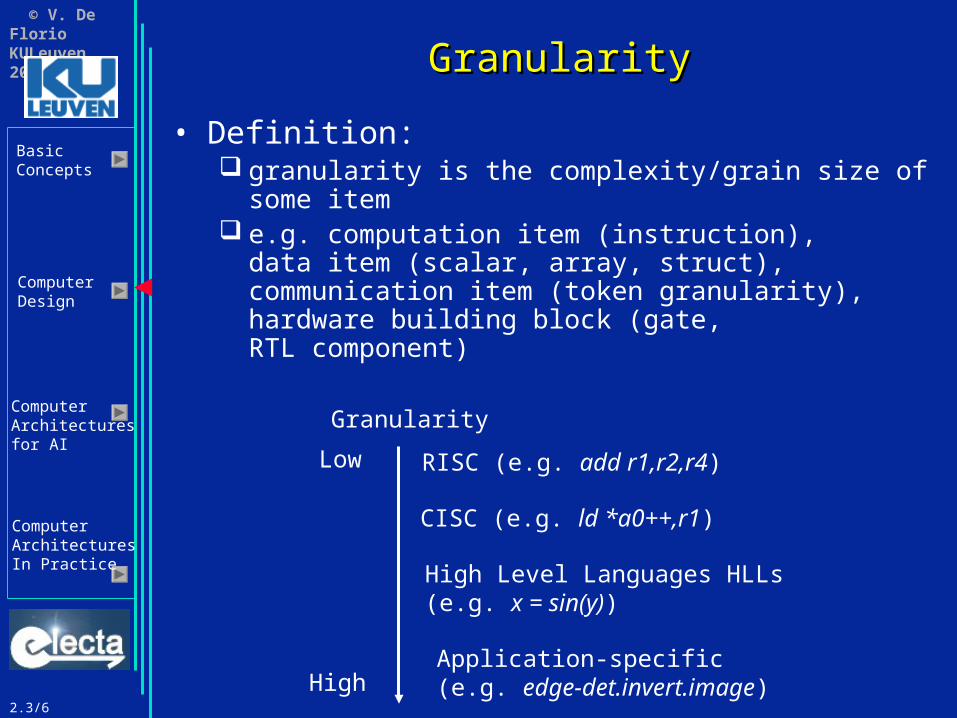
GranularityGranularity
• Definition: granularity is the complexity/grain size of
some item e.g. computation item (instruction),
data item (scalar, array, struct), communication item (token granularity), hardware building block (gate, RTL component)
RISC (e.g. add r1,r2,r4)
CISC (e.g. ld *a0++,r1)
High Level Languages HLLs(e.g. x = sin(y))
Application-specific(e.g. edge-det.invert.image)
Low
High
Granularity

2.3/7
© V. De FlorioKULeuven 2002
BasicConcepts
ComputerDesign
ComputerArchitecturesfor AI
ComputerArchitecturesIn Practice
GranularityGranularity
• Deciding the granularity is an important design choice
• E.g. grain size for the communication tokens in a parallel computer: coarse grain: less communication overhead fine grain: less time penalty when two
communication packets compete for transmission over the same channel and collide

2.3/13
© V. De FlorioKULeuven 2002
BasicConcepts
ComputerDesign
ComputerArchitecturesfor AI
ComputerArchitecturesIn Practice
ParallelismParallelism
• Introduction to parallel processing Basic concepts: granularity, program, process,
thread Types of parallelism
• Instruction level parallelism

2.3/14
© V. De FlorioKULeuven 2002
BasicConcepts
ComputerDesign
ComputerArchitecturesfor AI
ComputerArchitecturesIn Practice
Types of parallelismTypes of parallelism
• Functional parallelism Different computations have to be performed on
the same or different data E.g. Multiple users submit jobs to the same
computer or a single user submits multiple jobs to the same computer
this is functional parallelism at the process leveltaken care of at run-time by the OS
Important for the exam!

2.3/17
© V. De FlorioKULeuven 2002
BasicConcepts
ComputerDesign
ComputerArchitecturesfor AI
ComputerArchitecturesIn Practice
Types of parallelismTypes of parallelism
• Data parallelism Same computations have to be performed on a
whole set of data E.g. 2D convolution of an image
This is data parallelism at the loop level: consecutive loop iterations are candidates for parallel execution, subject to inter-iteration data dependencies
Leads often to massive amount of parallelism
Important for the exam!

2.3/18
© V. De FlorioKULeuven 2002
BasicConcepts
ComputerDesign
ComputerArchitecturesfor AI
ComputerArchitecturesIn Practice
Levels of parallelismLevels of parallelism
• Instruction level parallel (ILP) Functional parallelism at the instruction level Example: pipelining
• Data level parallel (DLP) Data parallelism at the loop level
• Process & thread level parallel (TLP) Functional parallelism at the thread and process
level

2.3/19
© V. De FlorioKULeuven 2002
BasicConcepts
ComputerDesign
ComputerArchitecturesfor AI
ComputerArchitecturesIn Practice
ParallelismParallelism
• Introduction to parallel processing• Instruction level parallelism
Introduction VLIW Advanced pipelining techniques Super scalar

2.3/20
© V. De FlorioKULeuven 2002
BasicConcepts
ComputerDesign
ComputerArchitecturesfor AI
ComputerArchitecturesIn Practice
ParallelismParallelism
• Introduction to parallel processing• Instruction level parallelism
Introduction VLIW Advanced pipelining techniques Super scalar

2.3/21
© V. De FlorioKULeuven 2002
BasicConcepts
ComputerDesign
ComputerArchitecturesfor AI
ComputerArchitecturesIn Practice
Type of Instruction Level Parallelism Type of Instruction Level Parallelism utilizationutilization
• Sequential instruction issuing, sequential instruction execution von Neumann processors
EU
Instruction word
2.3/22
© V. De FlorioKULeuven 2002
BasicConcepts
ComputerDesign
ComputerArchitecturesfor AI
ComputerArchitecturesIn Practice
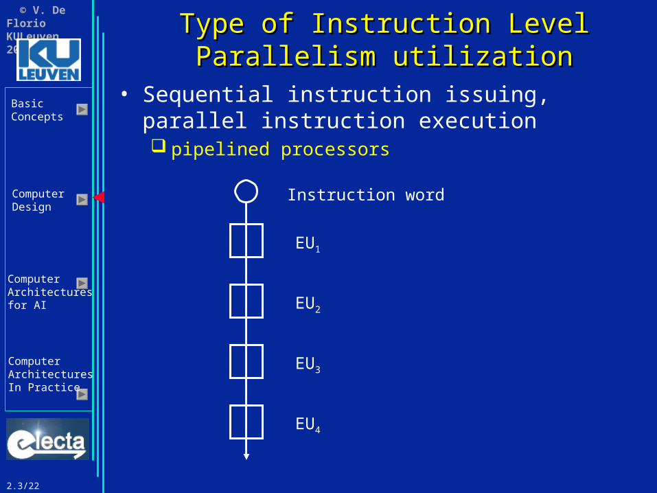
Type of Instruction Level Parallelism Type of Instruction Level Parallelism utilizationutilization
• Sequential instruction issuing, parallel instruction execution pipelined processors
EU1
EU2
EU3
EU4
Instruction word

2.3/23
© V. De FlorioKULeuven 2002
BasicConcepts
ComputerDesign
ComputerArchitecturesfor AI
ComputerArchitecturesIn Practice
Type of Instruction Level Parallelism Type of Instruction Level Parallelism utilizationutilization
• Parallel instruction issuing – compile-time determined by compiler, parallel instruction execution VLIW processors:
Very Long Instruction Word
EU1 EU2 EU3 EU4
Instruction word
2.3/24
© V. De FlorioKULeuven 2002
BasicConcepts
ComputerDesign
ComputerArchitecturesfor AI
ComputerArchitecturesIn Practice
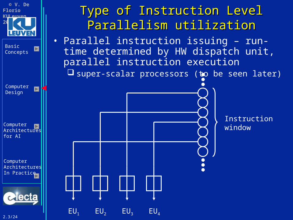
Type of Instruction Level Parallelism Type of Instruction Level Parallelism utilizationutilization
• Parallel instruction issuing – run-time determined by HW dispatch unit, parallel instruction execution super-scalar processors (to be seen later)
EU1 EU2 EU3 EU4
Instructionwindow

2.3/25
© V. De FlorioKULeuven 2002
BasicConcepts
ComputerDesign
ComputerArchitecturesfor AI
ComputerArchitecturesIn Practice
Type of Instruction Level Parallelism Type of Instruction Level Parallelism utilizationutilization
• Most processors provide sequential execution semantics regardless how the processor actually executes the
instructions (sequential or parallel, in-order or out-of-order), the result is the same as sequential execution in the order they were written
• VLIW and IA-64 provide parallel execution semantics explicit indication in ASM which
instructions are executed in parallel

2.3/26
© V. De FlorioKULeuven 2002
BasicConcepts
ComputerDesign
ComputerArchitecturesfor AI
ComputerArchitecturesIn Practice
ParallelismParallelism
• Introduction to parallel processing• Instruction level parallelism
Introduction VLIW Advanced pipelining techniques Super scalar

2.3/27
© V. De FlorioKULeuven 2002
BasicConcepts
ComputerDesign
ComputerArchitecturesfor AI
ComputerArchitecturesIn Practice
VLIWVLIW
EU EU EU EU
Dec
Instruction Register
Dec Dec Dec
Main instructionmemory
128 bit
Instruction Cache
128 bit
32 bit each
256 decoded bits each
Register file32 bit each; 8 read ports, 4 write ports
Cach
e/
RA
M
32 bit each; 2 read ports, 1 write port
Main datamemory
32 bit;1 bi-directional port

2.3/28
© V. De FlorioKULeuven 2002
BasicConcepts
ComputerDesign
ComputerArchitecturesfor AI
ComputerArchitecturesIn Practice
VLIWVLIW
• Properties Multiple Execution Units: multiple instructions
issued in one clock cycle Every EU requires 2 operands and delivers one
result every clock cycle: high data memory bandwidth needed
Careful design of data memory hierarchyRegister file with many portsLarge register file: 64-256 registersCarefully balanced cache/RAM hierarchy with
decreasing number of ports and increasing memory size and access time for the higher levels (IMEC research: DTSE)

2.3/31
© V. De FlorioKULeuven 2002
BasicConcepts
ComputerDesign
ComputerArchitecturesfor AI
ComputerArchitecturesIn Practice
VLIWVLIW
• Properties Compiler should determine which instructions can
be issued in a single cycle without control dependency conflict nor data dependency conflict
Deterministic utilization of parallelism: good for hard-real-time
Compile-time analysis of source code: worst case analysis instead of actual case
Very sophisticated compilers, especially when the EUs are pipelined! Perform well since early 2000

2.3/32
© V. De FlorioKULeuven 2002
BasicConcepts
ComputerDesign
ComputerArchitecturesfor AI
ComputerArchitecturesIn Practice
VLIWVLIW
• Properties Compiler should determine which instructions can
be issued in a single cycle without control dependency conflict nor data dependency conflict
Very difficult to write assembly: programmer should resolve all control flow conflicts all data flow conflicts all pipelining conflicts and at the same time fit data accesses into the available
data memory bandwidth and all program accesses into the available program
memory bandwidth e.g. 2 weeks for a sum-of-products (3 lines of C-code)
All high end DSP processors since 1999 are VLIW processors (examples: Philips Trimedia -- high end TV, TI TMS320C6x -- GSM base stations and ISP modem arrays)
2.3/33
© V. De FlorioKULeuven 2002
BasicConcepts
ComputerDesign
ComputerArchitecturesfor AI
ComputerArchitecturesIn Practice
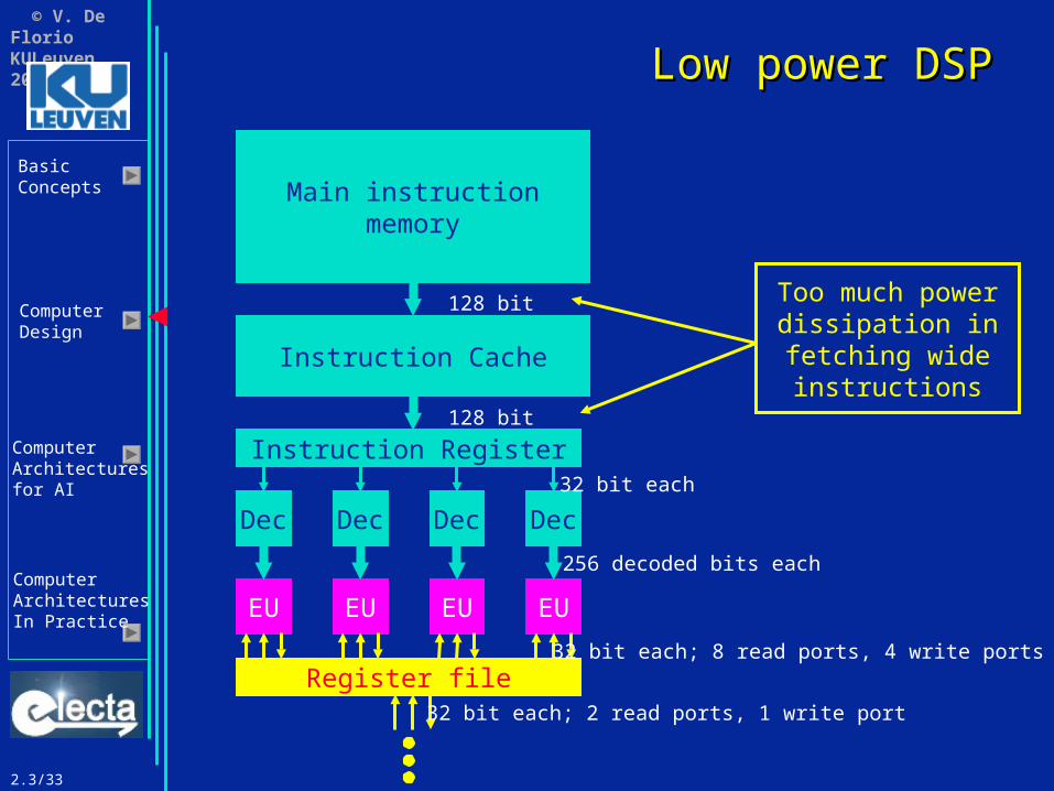
Low power DSPLow power DSP
EU EU EU EU
Dec
Instruction Register
Dec Dec Dec
Main instructionmemory
128 bit
Instruction Cache
128 bit
32 bit each
256 decoded bits each
Register file32 bit each; 8 read ports, 4 write ports
32 bit each; 2 read ports, 1 write port
Too much powerdissipation infetching wideinstructions

2.3/34
© V. De FlorioKULeuven 2002
BasicConcepts
ComputerDesign
ComputerArchitecturesfor AI
ComputerArchitecturesIn Practice
Low power DSPLow power DSP
EU EU EU EU
Dec
Instruction Register
Dec Dec Dec
24 bitICach
e
128 bit
32 bit each
256 decoded bits each
Register file32 bit each; 8 read ports, 4 write ports
32 bit each; 2 read ports, 1 write port
Instructionexpansion
Main
IMem
24 bit
E.g. ADD4 is expanded intoADD || ADD || ADD || ADD

2.3/35
© V. De FlorioKULeuven 2002
BasicConcepts
ComputerDesign
ComputerArchitecturesfor AI
ComputerArchitecturesIn Practice
Low power DSPLow power DSP
• Properties Power consumption in program memory is reduced
by specializing the instructions for the application Not all combinations of all instructions for the EUs
are possible, but only a limited set, i.e. those combinations that lead to a substantial speed-up of the application
Those relevant combinations are represented by the smallest possible amount of bits to reduce program memory width and hence program memory power consumption
Can only be done for embedded DSP applications: processor is specialized for 1 application (examples: TI TMS320C54x -- GSM mobile phones, TI TMS320C55x -- UMTS mobile phones)

2.3/36
© V. De FlorioKULeuven 2002
BasicConcepts
ComputerDesign
ComputerArchitecturesfor AI
ComputerArchitecturesIn Practice
Low power DSP for Low power DSP for interactiveinteractivemultimediamultimedia
REU REU REU REU
Dec
Instruction Register
Dec Dec Dec
24 bitICach
e
128 bit
32 bit each
256 decoded bits each
Register file32 bit each; 8 read ports, 4 write ports
32 bit each; 2 read ports, 1 write port
ReconfigurableInstruction expansion
Main
IMem
24 bit Run-time reconfigurationallows to adapt specialization
to changing applicationrequirements

2.3/38
© V. De FlorioKULeuven 2002
BasicConcepts
ComputerDesign
ComputerArchitecturesfor AI
ComputerArchitecturesIn Practice
ParallelismParallelism
• Introduction to parallel processing• Instruction level parallelism
Introduction VLIW Advanced pipelining techniques Super scalar

2.3/39
© V. De FlorioKULeuven 2002
BasicConcepts
ComputerDesign
ComputerArchitecturesfor AI
ComputerArchitecturesIn Practice
Advanced PipeliningAdvanced Pipelining
• Pipeline CPI is the result of many components
• A number of techniques act on one or more of these components: Loop unrolling Scoreboarding Dynamic branch prediction Speculation …
• To be seen later
CPUTIME(p) = IC(p) CPI(p) clock rate

2.3/40
© V. De FlorioKULeuven 2002
BasicConcepts
ComputerDesign
ComputerArchitecturesfor AI
ComputerArchitecturesIn Practice
Advanced PipeliningAdvanced Pipelining
• Till now, Instruction-level parallelism was searched within the boundaries of a basic block (BB)
• A BB is 6-7 instructions on average too small to reach the expected performance• What is worse, there’s a big chance that
these instructions have dependencies Even less performance can be expected

2.3/41
© V. De FlorioKULeuven 2002
BasicConcepts
ComputerDesign
ComputerArchitecturesfor AI
ComputerArchitecturesIn Practice
Advanced PipeliningAdvanced Pipelining
• To obtain more, we need to go beyond the BB limitation:
• We must exploit ILP across multiple BB’s• Simplest way: loop level parallelism (LLP):
Exploiting the parallelism among iterations of a loop
• Converting LLP into ILP Loop unrolling
Statically (compiler-based)Dynamically (HW-based)
• Using vector instructions Does not require LLP -> ILP conversion

2.3/42
© V. De FlorioKULeuven 2002
BasicConcepts
ComputerDesign
ComputerArchitecturesfor AI
ComputerArchitecturesIn Practice
Advanced PipeliningAdvanced Pipelining
• The efficiency of the conversion depends On the amount of ILP available On latencies of the functional units in the pipeline On the ability to avoid pipeline stalls by separating
dependent instructions by a “distance” (in terms of stages) equal to the latency peculiar to the source instruction
LW LW xx, …, …
INSTR …, INSTR …, xx
a load must not be followed by the immediate a load must not be followed by the immediate use of the load destination registeruse of the load destination register

2.3/43
© V. De FlorioKULeuven 2002
BasicConcepts
ComputerDesign
ComputerArchitecturesfor AI
ComputerArchitecturesIn Practice
Advanced Pipelining Advanced Pipelining Loop unrollingLoop unrolling
Assumptions and steps1. We assume the following latencies
ProducerInstruction
C onsum erInstruction
Latency
FP ALU O P FP ALU O P 3
FP ALU O P STO RE DBL 2
LO AD DBL FP ALU O P 1
LO AD DBL STO RE DBL 0

2.3/44
© V. De FlorioKULeuven 2002
BasicConcepts
ComputerDesign
ComputerArchitecturesfor AI
ComputerArchitecturesIn Practice
Advanced Pipelining Advanced Pipelining Loop unrollingLoop unrolling
2. We assume to work with a simple loop such as
for (I=1; I<=1000; I++) x[I] = X[I] + s;
• Note: each iteration is independent of the others
Very simple case

2.3/45
© V. De FlorioKULeuven 2002
BasicConcepts
ComputerDesign
ComputerArchitecturesfor AI
ComputerArchitecturesIn Practice
Advanced Pipelining Advanced Pipelining Loop unrollingLoop unrolling
3. Translated in DLX, this simple loop looks like this:
; assumptions: R1 = &x[1000]; F2 = sLoop: LD F0, 0(R1) ; F0 = x[I]
ADDD F4, F0, F2 ; F4 = F0 + s SD 0(R1), F4 ; store result SUBI R1, R1, #8 ; R1 = R1 - 1 BNEZ R1, Loop ; if (R1) ; goto Loop
W
O
2.3/46
© V. De FlorioKULeuven 2002
BasicConcepts
ComputerDesign
ComputerArchitecturesfor AI
ComputerArchitecturesIn Practice
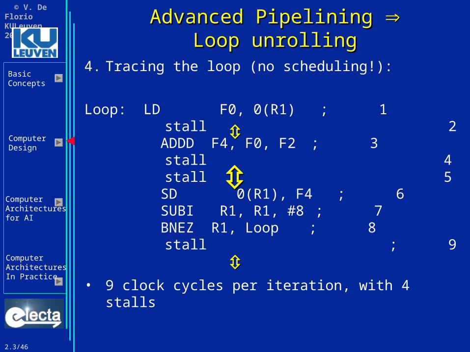
4. Tracing the loop (no scheduling!):
Loop: LD F0, 0(R1) ; 1 stall 2 ADDD F4, F0, F2 ; 3 stall 4 stall 5 SD 0(R1), F4 ; 6 SUBI R1, R1, #8 ; 7 BNEZ R1, Loop ; 8 stall ; 9
• 9 clock cycles per iteration, with 4 stalls
Advanced Pipelining Advanced Pipelining Loop unrollingLoop unrolling
2.3/47
© V. De FlorioKULeuven 2002
BasicConcepts
ComputerDesign
ComputerArchitecturesfor AI
ComputerArchitecturesIn Practice
Advanced Pipelining Advanced Pipelining Loop unrollingLoop unrolling
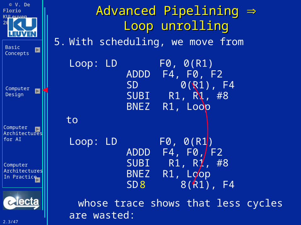
5. With scheduling, we move from
Loop: LD F0, 0(R1) ADDD F4, F0, F2 SD 0(R1), F4 SUBI R1, R1, #8 BNEZ R1, Loop
to
Loop: LD F0, 0(R1) ADDD F4, F0, F2 SUBI R1, R1, #8 BNEZ R1, Loop SD 8(R1), F48
whose trace shows that less cycles are wasted:

2.3/48
© V. De FlorioKULeuven 2002
BasicConcepts
ComputerDesign
ComputerArchitecturesfor AI
ComputerArchitecturesIn Practice
Advanced Pipelining Advanced Pipelining Loop unrollingLoop unrolling
6. Tracing the loop (with scheduling!):
Loop: LD F0, 0(R1) ; 1 stall 2 ADDD F4, F0, F2 ; 3 SUBI R1, R1, 8 ; 4 BNEZ R1, Loop ; 5 SD 8(R1), F4 ; 6
• 6 clock cycles per iteration, with 1 stall• 3 stalls less!• Still the useful cycles are just 3• How to gain more?
O
O

2.3/49
© V. De FlorioKULeuven 2002
BasicConcepts
ComputerDesign
ComputerArchitecturesfor AI
ComputerArchitecturesIn Practice
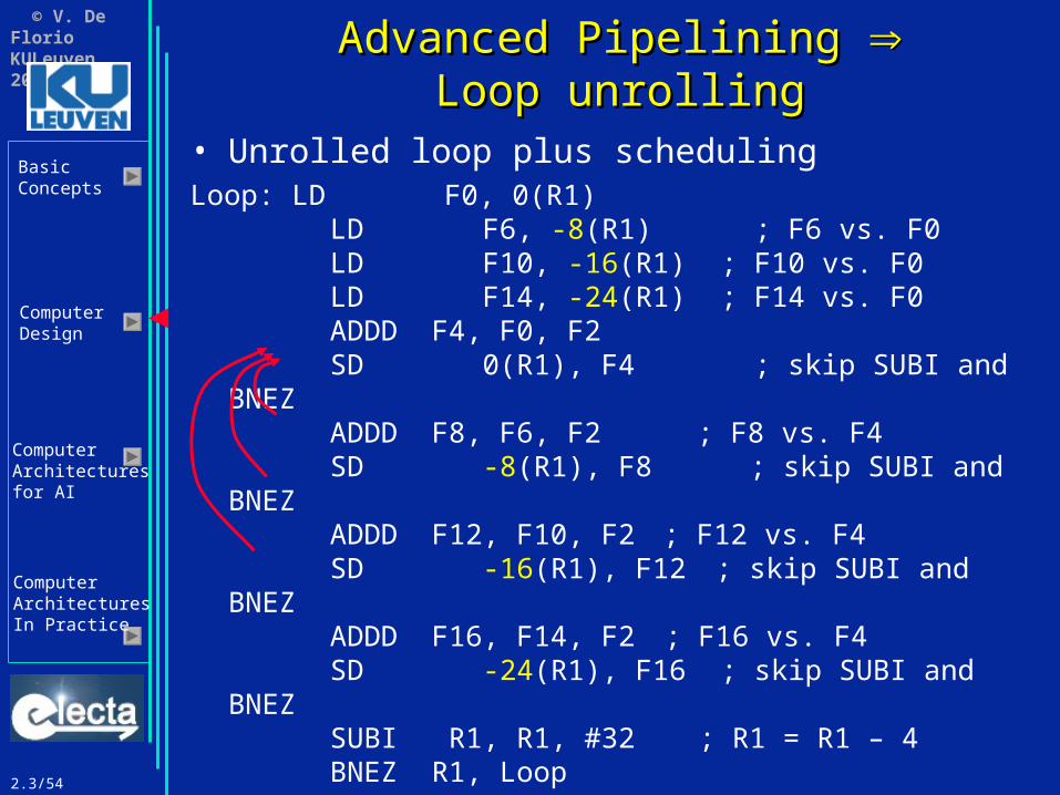
Advanced Pipelining Advanced Pipelining Loop unrollingLoop unrolling
7. With loop unrolling: replicating the body of loop multiple times
Loop: LD F0, 0(R1) ADDD F4, F0, F2 SD 0(R1), F4 ; skip SUBI and BNEZ LD F6, -8(R1) ; F6 vs. F0 ADDD F8, F6, F2 ; F8 vs. F4 SD -8(R1), F8 ; skip SUBI and BNEZ LD F10, -16(R1) ; F10 vs. F0 ADDD F12, F10, F2 ; F12 vs. F4 SD -16(R1), F12 ; skip SUBI and BNEZ LD F14, -24(R1) ; F14 vs. F0 ADDD F16, F14, F2 ; F16 vs. F4 SD -24(R1), F16 ; skip SUBI and BNEZ SUBI R1, R1, #32 ; R1 = R1 – 4 BNEZ R1, Loop
• Spared 3 x (SUBI + BNEZ)

2.3/50
© V. De FlorioKULeuven 2002
BasicConcepts
ComputerDesign
ComputerArchitecturesfor AI
ComputerArchitecturesIn Practice
Advanced Pipelining Advanced Pipelining Loop unrollingLoop unrolling
• Loop unrolling: replicating the body of loop multiple times
Some branches are eliminated The ratio w/o increases
The BB artificially increases its size Higher probability of optimal scheduling
Requires a wider set of registers and adjusting values of load and store registers
(In the given example,) Every operation is followed by a dependent instruction Will cause a stall Trace of unscheduled unrolled loop: 27 cycles
2 per LD, 3 per ADD, 2 per branch, 1 per any other 6.8 clock cycles per iterationPure scheduling is better! (6 cycles)

2.3/51
© V. De FlorioKULeuven 2002
BasicConcepts
ComputerDesign
ComputerArchitecturesfor AI
ComputerArchitecturesIn Practice
Advanced Pipelining Advanced Pipelining Loop unrollingLoop unrolling
• Unrolled loop plus schedulingLoop: LD F0, 0(R1)
ADDD F4, F0, F2 SD 0(R1), F4 ; skip SUBI and BNEZ LD F6, -8(R1) ; F6 vs. F0 ADDD F8, F6, F2 ; F8 vs. F4 SD -8(R1), F8 ; skip SUBI and BNEZ LD F10, -16(R1) ; F10 vs. F0 ADDD F12, F10, F2 ; F12 vs. F4 SD -16(R1), F12 ; skip SUBI and BNEZ LD F14, -24(R1) ; F14 vs. F0 ADDD F16, F14, F2 ; F16 vs. F4 SD -24(R1), F16 ; skip SUBI and BNEZ SUBI R1, R1, #32 ; R1 = R1 – 4 BNEZ R1, Loop

2.3/52
© V. De FlorioKULeuven 2002
BasicConcepts
ComputerDesign
ComputerArchitecturesfor AI
ComputerArchitecturesIn Practice
Advanced Pipelining Advanced Pipelining Loop unrollingLoop unrolling
• Unrolled loop plus schedulingLoop: LD F0, 0(R1)
LD F6, -8(R1) ; F6 vs. F0 ADDD F4, F0, F2 SD 0(R1), F4 ; skip SUBI and BNEZ ADDD F8, F6, F2 ; F8 vs. F4 SD -8(R1), F8 ; skip SUBI and BNEZ LD F10, -16(R1) ; F10 vs. F0 ADDD F12, F10, F2 ; F12 vs. F4 SD -16(R1), F12 ; skip SUBI and BNEZ LD F14, -24(R1) ; F14 vs. F0 ADDD F16, F14, F2 ; F16 vs. F4 SD -24(R1), F16 ; skip SUBI and BNEZ SUBI R1, R1, #32 ; R1 = R1 – 4 BNEZ R1, Loop

2.3/53
© V. De FlorioKULeuven 2002
BasicConcepts
ComputerDesign
ComputerArchitecturesfor AI
ComputerArchitecturesIn Practice
Advanced Pipelining Advanced Pipelining Loop unrollingLoop unrolling
• Unrolled loop plus schedulingLoop: LD F0, 0(R1)
LD F6, -8(R1) ; F6 vs. F0 LD F10, -16(R1) ; F10 vs. F0 ADDD F4, F0, F2 SD 0(R1), F4 ; skip SUBI and BNEZ ADDD F8, F6, F2 ; F8 vs. F4 SD -8(R1), F8 ; skip SUBI and BNEZ ADDD F12, F10, F2 ; F12 vs. F4 SD -16(R1), F12 ; skip SUBI and BNEZ LD F14, -24(R1) ; F14 vs. F0 ADDD F16, F14, F2 ; F16 vs. F4 SD -24(R1), F16 ; skip SUBI and BNEZ SUBI R1, R1, #32 ; R1 = R1 – 4 BNEZ R1, Loop
2.3/54
© V. De FlorioKULeuven 2002
BasicConcepts
ComputerDesign
ComputerArchitecturesfor AI
ComputerArchitecturesIn Practice
Advanced Pipelining Advanced Pipelining Loop unrollingLoop unrolling
• Unrolled loop plus schedulingLoop: LD F0, 0(R1)
LD F6, -8(R1) ; F6 vs. F0 LD F10, -16(R1) ; F10 vs. F0 LD F14, -24(R1) ; F14 vs. F0 ADDD F4, F0, F2 SD 0(R1), F4 ; skip SUBI and BNEZ ADDD F8, F6, F2 ; F8 vs. F4 SD -8(R1), F8 ; skip SUBI and BNEZ ADDD F12, F10, F2 ; F12 vs. F4 SD -16(R1), F12 ; skip SUBI and BNEZ ADDD F16, F14, F2 ; F16 vs. F4 SD -24(R1), F16 ; skip SUBI and BNEZ SUBI R1, R1, #32 ; R1 = R1 – 4 BNEZ R1, Loop

2.3/55
© V. De FlorioKULeuven 2002
BasicConcepts
ComputerDesign
ComputerArchitecturesfor AI
ComputerArchitecturesIn Practice
Advanced Pipelining Advanced Pipelining Loop unrollingLoop unrolling
• Unrolled loop plus schedulingLoop: LD F0, 0(R1)
LD F6, -8(R1) ; F6 vs. F0 LD F10, -16(R1) ; F10 vs. F0 LD F14, -24(R1) ; F14 vs. F0 ADDD F4, F0, F2 ADDD F8, F6, F2 ; F8 vs. F4
ADDD F12, F10, F2 ; F12 vs. F4 ADDD F16, F14, F2 ; F16 vs. F4 SD 0(R1), F4 ; skip SUBI and BNEZ SD -8(R1), F8 ; skip SUBI and BNEZ SD -16(R1), F12 ; skip SUBI and BNEZ SD -24(R1), F16 ; skip SUBI and BNEZ SUBI R1, R1, #32 ; R1 = R1 – 4 BNEZ R1, Loop
• 14 clock cycles, or 3.5 clock cycles / iteration
Enough distanceto prevent thedependency to turninto a hazard

2.3/56
© V. De FlorioKULeuven 2002
BasicConcepts
ComputerDesign
ComputerArchitecturesfor AI
ComputerArchitecturesIn Practice
Advanced Pipelining Advanced Pipelining Loop unrollingLoop unrolling
• Unrolling the loop exposes more computation that can be scheduled to minimize the stalls
• Unrolling increases the BB; as a result, a better choice can be done for scheduling
• A useful technique with two key requirements: Understanding how an instruction depends on
another Understanding how to change or reorder the
instructions, given the dependencies
• In what follows we concentrate on .

2.3/57
© V. De FlorioKULeuven 2002
BasicConcepts
ComputerDesign
ComputerArchitecturesfor AI
ComputerArchitecturesIn Practice
Loop unrolling: Loop unrolling: . dependencies. dependencies
• Again, let ( Ik)1 k IC(p) be the ordered series of instructions executed during the run of program p
• Given two instructions, Ii and Ij, with i<j, we say that Ij is dependent on Ii (Ii Ij) iff
R(Ii) D(Ij) R is the range and D the domain of a given instruction Ii produces a result which is consumed by Ij
or
n { 1,…,IC(p)} and k1 < k2 < … < kn such that Ii Ik1
Ik2 Ikn
Ij

2.3/58
© V. De FlorioKULeuven 2002
BasicConcepts
ComputerDesign
ComputerArchitecturesfor AI
ComputerArchitecturesIn Practice
Loop unrolling: Loop unrolling: . dependencies. dependencies
• (Ii Ik1 Ik2
…Ikn Ij) is called a dependency
(transitive) chain• Note that a dependency chain can be as long
as the entire execution of p
• A hazard implies dependency• Dependency does not imply a hazard!
• Scheduling tries to place dependent instructions in places where no hazard can occur

2.3/59
© V. De FlorioKULeuven 2002
BasicConcepts
ComputerDesign
ComputerArchitecturesfor AI
ComputerArchitecturesIn Practice
Loop unrolling: Loop unrolling: . dependencies. dependencies
• For instance: SUBI R1, R1, #8
BNEZ R1, Loop• This is clearly a dependence, but it does not
result in a hazard Forwarding eliminates the hazard
• Another example: LD F0, 0(R1) ADDD F4, F0, F2
• This is a data dependency which does lead to a hazard and a stall

2.3/60
© V. De FlorioKULeuven 2002
BasicConcepts
ComputerDesign
ComputerArchitecturesfor AI
ComputerArchitecturesIn Practice
Loop unrolling: Loop unrolling: . dependencies. dependencies
• Dealing with data dependencies• Two classes of methods:1. Keeping the dependence though avoiding
the hazard (via scheduling)2. Eliminating a dependence by transforming
the code

2.3/61
© V. De FlorioKULeuven 2002
BasicConcepts
ComputerDesign
ComputerArchitecturesfor AI
ComputerArchitecturesIn Practice
Loop unrolling: Loop unrolling: . dependencies. dependencies
• Class 2 implies more work• These are optimization methods used by the
compilers• Detecting dependencies when only using
registers is easy; the difficulties come from detecting dependencies in memory:
• For instance 100(R4) and 20(R6) may point to the same memory location
• Also the opposite situation may take place: LD 20(R4), R2 … ADD R3, R1, 20(R4)
• If R4 changes, this is no dependency

2.3/62
© V. De FlorioKULeuven 2002
BasicConcepts
ComputerDesign
ComputerArchitecturesfor AI
ComputerArchitecturesIn Practice
Loop unrolling: Loop unrolling: . dependencies. dependencies
• Ii Ij means that Ii produces a result that is consumed by Ij
• When there is no such production, e.g., Ii and Ij are both loads or stores, we call this a name dependency
• Two types of name dependencies: Antidependence
Corresponds to WAR hazardsIj x ; Ii x (reordering implies an error)
Output dependenceCorresponds to WAW hazardsIj x ; Ii x (reordering implies an error)
• No value is transferred between the instructions
• Register renaming solves the problem

2.3/63
© V. De FlorioKULeuven 2002
BasicConcepts
ComputerDesign
ComputerArchitecturesfor AI
ComputerArchitecturesIn Practice
Loop unrolling: Loop unrolling: . dependencies. dependencies
• Register renaming: if the register name is changed, the conflict disappears
• This technique can be either static (and done by the compiler) or dynamic (done by the HW)
• Let us consider again the following loop: Loop: LD F0, 0(R1)
ADDD F4, F0, F2 SD 0(R1), F4 SUBI R1, R1, #8 BNEZ R1, Loop
• Let us perform unrolling w/o renaming:

2.3/64
© V. De FlorioKULeuven 2002
BasicConcepts
ComputerDesign
ComputerArchitecturesfor AI
ComputerArchitecturesIn Practice
Loop unrolling: Loop unrolling: . dependencies. dependencies
Loop: LD F0, 0(R1) ADDD F4, F0, F2 SD 0(R1), F4 LD F0, -8(R1) ADDD F4, F0, F2 SD -8(R1), F4 LD F0, -16(R1) ADDD F4, F0, F2 SD -16(R1), F4 LD F0, -24(R1) ADDD F4, F0, F2 SD -24(R1), F0 SUBI R1, R1, #32 BNEZ R1, Loop
The yellow arrowsare name depen-dencies. To solvethem, we performrenaming

2.3/65
© V. De FlorioKULeuven 2002
BasicConcepts
ComputerDesign
ComputerArchitecturesfor AI
ComputerArchitecturesIn Practice
Loop unrolling: Loop unrolling: . dependencies. dependencies
Loop: LD F0, 0(R1) ADDD F4, F0, F2 SD 0(R1), F4 LD F6, -8(R1) ADDD F8, F6, F2 SD -8(R1), F8 LD F0, -16(R1) ADDD F4, F0, F2 SD -16(R1), F4 LD F0, -24(R1) ADDD F4, F0, F2 SD -24(R1), F0 SUBI R1, R1, #32 BNEZ R1, Loop

2.3/66
© V. De FlorioKULeuven 2002
BasicConcepts
ComputerDesign
ComputerArchitecturesfor AI
ComputerArchitecturesIn Practice
Loop unrolling: Loop unrolling: . dependencies. dependencies
Loop: LD F0, 0(R1) ADDD F4, F0, F2 SD 0(R1), F4 LD F6, -8(R1) ADDD F8, F6, F2 SD -8(R1), F8 LD F10, -16(R1) ADDD F12, F10, F2 SD -16(R1), F12 LD F14, -24(R1) ADDD F16, F14, F2 SD -24(R1), F16 SUBI R1, R1, #32 BNEZ R1, Loop

2.3/67
© V. De FlorioKULeuven 2002
BasicConcepts
ComputerDesign
ComputerArchitecturesfor AI
ComputerArchitecturesIn Practice
Loop unrolling: Loop unrolling: . dependencies. dependencies
Loop: LD F0, 0(R1) ADDD F4, F0, F2 SD 0(R1), F4 LD F6, -8(R1) ADDD F8, F6, F2 SD -8(R1), F8 LD F10, -16(R1) ADDD F12, F10, F2 SD -16(R1), F12 LD F14, -24(R1) ADDD F16, F14, F2 SD -24(R1), F16 SUBI R1, R1, #32 BNEZ R1, Loop
The yellow arrowsare data depen-dencies. To solvethem, we reorderthe instructions

2.3/68
© V. De FlorioKULeuven 2002
BasicConcepts
ComputerDesign
ComputerArchitecturesfor AI
ComputerArchitecturesIn Practice
Loop unrolling: Loop unrolling: . dependencies. dependencies
• A third class of dependencies is the one of control dependencies
• Examples: if (p1) s1; if (p2) s2;then p1 c s1 (s1 is control dependent on p1) p2 c s2 (s2 is control dependent on p2)
• Clearly p1 c s2 that is s2 is not control dependent on p1

2.3/71
© V. De FlorioKULeuven 2002
BasicConcepts
ComputerDesign
ComputerArchitecturesfor AI
ComputerArchitecturesIn Practice
Loop unrolling: Loop unrolling: . dependencies. dependencies
• Two properties are critical to control dependency: Exception behaviour Data flow
• Exception behaviour: suppose we have the following excerpt:
BEQZ R2, L1DIVI R1, 8(R2)
L1: …• We may be able to move the DIVI to before
the BEQZ without violating the sequential semantics of the program
• Suppose the branch is taken. Normally one would simply need to undo the DIVI
• What if DIVI triggers a DIVBYZERO exception?

2.3/72
© V. De FlorioKULeuven 2002
BasicConcepts
ComputerDesign
ComputerArchitecturesfor AI
ComputerArchitecturesIn Practice
Loop unrolling: Loop unrolling: . dependencies. dependencies
• Two properties are critical to control dependency: Exception behaviour Data flow
• Data flow must be preserved• Let us consider the following excerpt:
ADD R1, R2, R3BEQZ R4, LSUB R1, R5, R6
L: OR R7, R1, R8• Value of R1 depends on the control flow• The OR depends on both ADD and SUB• Also depends on the nature of the branch• R1 = (taken)? ADD.. : SUB..
2.3/73
© V. De FlorioKULeuven 2002
BasicConcepts
ComputerDesign
ComputerArchitecturesfor AI
ComputerArchitecturesIn Practice
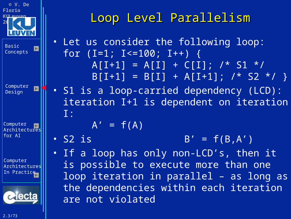
Loop Level ParallelismLoop Level Parallelism
• Let us consider the following loop:for (I=1; I<=100; I++) {
A[I+1] = A[I] + C[I]; /* S1 */B[I+1] = B[I] + A[I+1]; /* S2 */ }
• S1 is a loop-carried dependency (LCD):iteration I+1 is dependent on iteration I:
A’ = f(A)• S2 is B’ = f(B,A’)• If a loop has only non-LCD’s, then it is
possible to execute more than one loop iteration in parallel – as long as the dependencies within each iteration are not violated

2.3/74
© V. De FlorioKULeuven 2002
BasicConcepts
ComputerDesign
ComputerArchitecturesfor AI
ComputerArchitecturesIn Practice
Loop Level ParallelismLoop Level Parallelism
• What to do in the presence of LCD’s?• Loop transformations. Example:
for (I=1; I<=100; I++) { A[I+1] = A[I] + B[I]; /* S1 */B[I+1] = C[I] + D[I]; /* S2 */ }
• A’ = f(A, B) B’ = f(C, D)
• Note: no dependencies except LCD’s Instructions can be swapped!

2.3/75
© V. De FlorioKULeuven 2002
BasicConcepts
ComputerDesign
ComputerArchitecturesfor AI
ComputerArchitecturesIn Practice
Loop Level ParallelismLoop Level Parallelism
• What to do in the presence of LCD’s?• Loop transformations. Example:
for (I=1; I<=100; I++) { A[I+1] = A[I] + B[I]; /* S1 */B[I+1] = C[I] + D[I]; /* S2 */ }
• Note: the flow, i.e.,A0 B0 A0 B0C0 D0
C0 D0A1 B1 can be A1 B1
C1 D1 changed into C1 D1
A2 B2 A2 B2C2 D2 . . .
. . .

2.3/76
© V. De FlorioKULeuven 2002
BasicConcepts
ComputerDesign
ComputerArchitecturesfor AI
ComputerArchitecturesIn Practice
for (i=1; i <= 100; i=i+1) {A[i] = A[i] + B[i]; /* S1 */B[i+1] = C[i] + D[i]; /* S2 */
}
becomes
A[1] = A[1] + B[1];for (i=1; i <= 99; i=i+1) {
B[i+1] = C[i] + D[i];A[i+1] = A[i+1] + B[i+1];
}B[101] = C[100] + D[100];
Loop Level ParallelismLoop Level Parallelism

2.3/77
© V. De FlorioKULeuven 2002
BasicConcepts
ComputerDesign
ComputerArchitecturesfor AI
ComputerArchitecturesIn Practice
Loop Level ParallelimLoop Level Parallelim
• A’ = f(A, B) B’ = f(C, D)B’ = f(C, D) A’ = f(A’, B’)
• Now we have dependencies but no more LCD’s!
It is possible to execute more than one loop iteration in parallel – as long as the dependencies within each iteration are not violated

2.3/78
© V. De FlorioKULeuven 2002
BasicConcepts
ComputerDesign
ComputerArchitecturesfor AI
ComputerArchitecturesIn Practice
Dependency avoidanceDependency avoidance
1. “Batch” approaches: at compile time, the compiler schedules the instructions in order to minimize the dependencies (static scheduling)
2. “Interactive” approaches: at run-time, the HW rearranges the instructions in order to minimize the stalls (dynamic scheduling)
• Advantages of 2: Only approach when dependencies are only known
at run-time (pointers etc.) The compiler can be simpler Given an executable compiled for a machine with
machine-level X and pipeline organization Y, it can run efficiently on another machine with the same machine level but a different pipeline organization Z

2.3/79
© V. De FlorioKULeuven 2002
BasicConcepts
ComputerDesign
ComputerArchitecturesfor AI
ComputerArchitecturesIn Practice
Dynamic SchedulingDynamic Scheduling
• Static scheduling: compiler techniques for scheduling (rearranging) the instructions so to separate dependent instructions And hence minimize unsolvable hazards causing
unavoidable stalls
• Dynamic scheduling: HW-based, run-time techniques
• A dynamically scheduled processor does not try to remove true data dependencies (which would be impossible): it tries to avoid stalling when dependencies are present
• The two techniques can be both used

2.3/80
© V. De FlorioKULeuven 2002
BasicConcepts
ComputerDesign
ComputerArchitecturesfor AI
ComputerArchitecturesIn Practice
Dynamic Scheduling: General IdeaDynamic Scheduling: General Idea
• If an instruction is stalled in the pipeline, no later instruction can proceed
• A dependence between two instructions close to each other causes a stall
• A stall means that, even though there may be idle functional units that could potentially serve other instructions, those units have to stay idle
• Example:DIVD F0, F2, F4ADDD F10, F0, F8SUBD F12, F8, F14
• ADDD depends on DIVD; but SUBD does not. Despite this, it is not issued!

2.3/81
© V. De FlorioKULeuven 2002
BasicConcepts
ComputerDesign
ComputerArchitecturesfor AI
ComputerArchitecturesIn Practice
Dynamic Scheduling: General IdeaDynamic Scheduling: General Idea
• So SUBD is not issued even there might be a functional unit ready to perform the requested operation
• Big performance limitation!• What are the reasons that lead to this
problem?• In-order instruction issuing and execution:
instructions issue and execute one at a time, one after the other

2.3/82
© V. De FlorioKULeuven 2002
BasicConcepts
ComputerDesign
ComputerArchitecturesfor AI
ComputerArchitecturesIn Practice
Dynamic Scheduling: General IdeaDynamic Scheduling: General Idea
• Example: in DLX, the issue of an instruction occurs at ID (instruction decode)
• In DLX, ID checks for absence of structural hazards and waits for the absence of data hazards
• These two steps may be made distinct

2.3/83
© V. De FlorioKULeuven 2002
BasicConcepts
ComputerDesign
ComputerArchitecturesfor AI
ComputerArchitecturesIn Practice
Dynamic Scheduling: General IdeaDynamic Scheduling: General Idea
• The issue process gets divided into two parts:1. Checking the presence of structural hazards2. Waiting for the absence of a data hazard• Instructions are issued in order, but they
execute and complete as soon as their data operands are available
• Data flow approach

2.3/84
© V. De FlorioKULeuven 2002
BasicConcepts
ComputerDesign
ComputerArchitecturesfor AI
ComputerArchitecturesIn Practice
Dynamic Scheduling: General IdeaDynamic Scheduling: General Idea
• The ID pipeline stage is divided into two sub-stages:
• ID.1 (Issue) : decode the instruction, check for structural hazards
• ID.2 (read operands) : wait until no data hazards, then read operands

2.3/85
© V. De FlorioKULeuven 2002
BasicConcepts
ComputerDesign
ComputerArchitecturesfor AI
ComputerArchitecturesIn Practice
Dynamic Scheduling: General IdeaDynamic Scheduling: General Idea
• In the DLX floating point pipeline, the EX stage of instructions may take multiple cycles
• For each issued instruction I, depending on the resolution of structural and data hazards, I may be be waiting for resources or data, or in execution, or completed
• More than a single instruction can be in execution at the same time

2.3/86
© V. De FlorioKULeuven 2002
BasicConcepts
ComputerDesign
ComputerArchitecturesfor AI
ComputerArchitecturesIn Practice
ScoreboardingScoreboarding
• Scorebord (CDC6600, 1964): a technique to allow instructions to execute out of order when there are sufficient resources and no data dependencies
• Goal: execution rate of 1 instruction per clock cycle in the absence of structural hazards
• Large set of FUs:4 FPUs, 5 units for memory references7 integer FUs
Highly redundant (parallel) system
• Four steps replace the ID, EX, WB stages

2.3/87
© V. De FlorioKULeuven 2002
BasicConcepts
ComputerDesign
ComputerArchitecturesfor AI
ComputerArchitecturesIn Practice
ScoreboardingScoreboarding
• IF (a FU is available && no active instruction has same destination reg) {
issue I to the FU; update state; }
Avoids WAWs
• ASA (the two source operands are available in the registers) {
read operands;manage RAW stalls;
}• For each FU: ASA (operands are available)
{ start EX; EOX? Alert scoreboard; }
• When at WB: { wait for (no WAR hazards); store output to destination reg; }
Avoids WARs
2.3/88
© V. De FlorioKULeuven 2002
BasicConcepts
ComputerDesign
ComputerArchitecturesfor AI
ComputerArchitecturesIn Practice
ScoreboardingScoreboarding
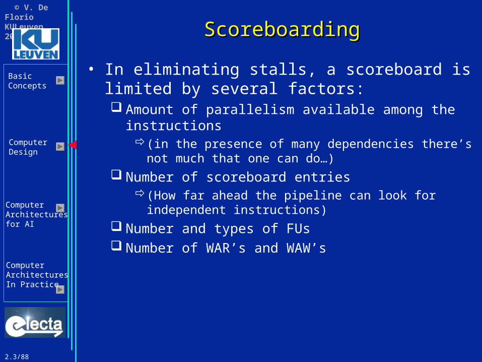
• In eliminating stalls, a scoreboard is limited by several factors: Amount of parallelism available among the
instructions(in the presence of many dependencies there’s not
much that one can do…) Number of scoreboard entries
(How far ahead the pipeline can look for independent instructions)
Number and types of FUs Number of WAR’s and WAW’s

2.3/89
© V. De FlorioKULeuven 2002
BasicConcepts
ComputerDesign
ComputerArchitecturesfor AI
ComputerArchitecturesIn Practice
ScoreboardingScoreboarding
• The effectiveness of the scoreboard heavily depends on the register file
• All operands are read from registers, all outputs go to destination registers
The availability of registers influence the capability to eliminate stalls

2.3/90
© V. De FlorioKULeuven 2002
BasicConcepts
ComputerDesign
ComputerArchitecturesfor AI
ComputerArchitecturesIn Practice
Tomasulo’s approachTomasulo’s approach
• Tomasulo’s approach (IBM 360/91, 1967) : An improvement of scoreboarding when a limited number of registers is allowed by a machine architecture
• Based on virtual registers• The IBM 360/91 had two key design goals:
To be faster than its predecessors To be machine level compatible with its
predecessors
• Problem: the 360 family had only 4 FP registers
• Tomasulo combined the key ideas of scoreboarding with register renaming

2.3/91
© V. De FlorioKULeuven 2002
BasicConcepts
ComputerDesign
ComputerArchitecturesfor AI
ComputerArchitecturesIn Practice
Tomasulo’s approachTomasulo’s approach
• IBM 360/91 FUs: 3 ADDD/SUBD, 2 MULD, 6 LD, 6 SD
• Key element: the reservation station (RS): a buffer which holds the operands of the instructions waiting to issue
• Key concept: A RS fetches and buffers an operand as soon as it is
available, eliminating the need to get that operand from a register
Instead of tracing the source and destination registers, we track source and destination RS’s
OP
RSa RSb
RSc

2.3/92
© V. De FlorioKULeuven 2002
BasicConcepts
ComputerDesign
ComputerArchitecturesfor AI
ComputerArchitecturesIn Practice
Tomasulo’s approachTomasulo’s approach
• A reservation station represents: A static data, read from a register A “live” data (a future data) that will be produced
by another RS and FU
• Hazard detection and execution control are not centralised into a scoreboard
• They are distributed in each RS, which, independently: Controls a FU attached to it, And starts that FU the moment the operands
become available

2.3/93
© V. De FlorioKULeuven 2002
BasicConcepts
ComputerDesign
ComputerArchitecturesfor AI
ComputerArchitecturesIn Practice
Tomasulo’s approachTomasulo’s approach
• The operands go to the FUs through the (wide set of) RS’s, not through the (small) register file
• This is managed through a broadcast that makes use of a common result-or-data bus
• All units waiting for an operand can load it at the same time:
RSa
OP OP2
RSd
RSc
RSb RSb
RSe

2.3/94
© V. De FlorioKULeuven 2002
BasicConcepts
ComputerDesign
ComputerArchitecturesfor AI
ComputerArchitecturesIn Practice
Tomasulo’s approachTomasulo’s approach
• The execution is driven by a graph of dependencies
RSa
SUBD MULTD
RSd
RSc
RSb
RSe
SUBD
RSf
SUBD
RSg
• A “live data structure” approach (similar to LINDA): a tuple is made available in the future, when a thread will have finished producing it

2.3/99
© V. De FlorioKULeuven 2002
BasicConcepts
ComputerDesign
ComputerArchitecturesfor AI
ComputerArchitecturesIn Practice
Major Advantages of Tomasulo’sMajor Advantages of Tomasulo’s
• Distributed approach: the RS’s independently control the FU’s
• Distributed hazard detection logic
• The CDB broadcasts results -> all pending instructions depending on that result are unblocked simultaneously The CDB, being a bus, reaches many destinations in
a single clock cycle If the waiting instructions get their missing operand
in that clock cycle, they can all begin execution on the next clock cycle
• WAR and WAW are eliminated by renaming registers using the RS’s

2.3/100
© V. De FlorioKULeuven 2002
BasicConcepts
ComputerDesign
ComputerArchitecturesfor AI
ComputerArchitecturesIn Practice
Reducing branch penaltiesReducing branch penalties
• Static ApproachesDynamic Approaches

2.3/101
© V. De FlorioKULeuven 2002
BasicConcepts
ComputerDesign
ComputerArchitecturesfor AI
ComputerArchitecturesIn Practice
Reducing branch penalties:Reducing branch penalties:Dynamic Branch PredictionDynamic Branch Prediction
• A branch history table
Address Branch Nature
0xA0B2DF37 BNEZ …
0xA0B2F02A BEQ …
0xA0B30504 BNEZ …
0xA0B30537 BGT …
37
2A
04
.
.
.
.
.
.
.
.
.
.
.
.
.
.
.
.
.
.
.
.
.
taken
taken
taken taken
untaken
untaken
untaken
un

2.3/102
© V. De FlorioKULeuven 2002
BasicConcepts
ComputerDesign
ComputerArchitecturesfor AI
ComputerArchitecturesIn Practice
Dynamic Branch Prediction Dynamic Branch Prediction Branch History Table Branch History Table Algorithm Algorithm
/* before the branch is evaluated */If (Current instruction is a branch) {
entry = PC & 0x000000FF;predict branch as ( BHT [ entry ] );
}
/* after the branch */If (branch was mispredicted)
BHT [ entry ] = 1 – BHT [ entry ]

2.3/103
© V. De FlorioKULeuven 2002
BasicConcepts
ComputerDesign
ComputerArchitecturesfor AI
ComputerArchitecturesIn Practice
Dynamic Branch Prediction Dynamic Branch Prediction Branch History Table Branch History Table Algorithm Algorithm
• Just one bit is enough for coding the Boolean value “taken” vs. “untaken”
• Note: the function associating addresses to entries in the BHT is not guaranteed to be a bijection (one-to-one relationship):
• The algorithm records the most recently behaviour of one or more branches For instance, entry 37 corresponds to two b.’s
• Despite this, the scheme works well…
• …though in some cases, the performance of the scheme is not that satisfactory:

2.3/104
© V. De FlorioKULeuven 2002
BasicConcepts
ComputerDesign
ComputerArchitecturesfor AI
ComputerArchitecturesIn Practice
Dynamic Branch Prediction Dynamic Branch Prediction Branch History Table Branch History Table Accuracy Accuracy
• for (i=0; i<BIGN; i++)for (j=0; j<9; j++)
{ do stg(); }
• Loop is taken nine times in a row then not taken once
• Taken 90%, Untaken 10%
• What is the prediction accuracy?

2.3/105
© V. De FlorioKULeuven 2002
BasicConcepts
ComputerDesign
ComputerArchitecturesfor AI
ComputerArchitecturesIn Practice
Dynamic Branch Prediction Dynamic Branch Prediction Branch History Table Branch History Table Accuracy Accuracy
Taken U 0Taken T 1. . .Taken T 1Untaken T 0Taken U 0Taken T 1. . .Taken T 1Untaken T 0Taken U 0Taken T 1. . .Taken T 1Untaken T 0Taken U 0
8 successful predictions
8 successful predictions
8 successful predictions
2 mispredictions
2 mispredictions
2 mispredictions
9
9
9
S.S. Prediction accuracy is just 80% !

2.3/106
© V. De FlorioKULeuven 2002
BasicConcepts
ComputerDesign
ComputerArchitecturesfor AI
ComputerArchitecturesIn Practice
Dynamic Branch Prediction Dynamic Branch Prediction Branch History Table Branch History Table Accuracy Accuracy
• Loop branches (taken n-1 times in a row, untaken once)
• Performance of this dynamic branch predictor (based on a single-bit prediction entry): Misprediction: 2 x 1 / n Twice rate of untaken branches

2.3/107
© V. De FlorioKULeuven 2002
BasicConcepts
ComputerDesign
ComputerArchitecturesfor AI
ComputerArchitecturesIn Practice
Dynamic Branch Prediction Dynamic Branch Prediction Two-bit Prediction SchemeTwo-bit Prediction Scheme
• Use a two bit field as a “branch behaviour recorder”
• Allow a state to change only when two mispredictions in a row occur:
Taken
Taken
Taken
Taken
N ot taken
N ot taken
N ot taken
N ot taken
Predict taken Predict taken
Predict not taken Predict not taken

2.3/108
© V. De FlorioKULeuven 2002
BasicConcepts
ComputerDesign
ComputerArchitecturesfor AI
ComputerArchitecturesIn Practice
Dynamic Branch Prediction Dynamic Branch Prediction Branch History Table Branch History Table Accuracy Accuracy
Taken U2 0Taken U 0Taken T2 1Taken T2 1. . .Taken T2 1Untaken T 0Taken T2 1. . .Taken T2 1Untaken T 0Taken T2 1. . .Taken T2 1
7 successful predictions
9 successful predictions
2 mispredictions first
S.S. Prediction accuracy is now 90%
9 successful predictions
STEADYSTATE

2.3/109
© V. De FlorioKULeuven 2002
BasicConcepts
ComputerDesign
ComputerArchitecturesfor AI
ComputerArchitecturesIn Practice
Dynamic Branch Prediction Dynamic Branch Prediction Branch History Table Branch History Table Accuracy Accuracy
18%
tom catv
spiceSPEC 89 benchm arks
gcc
li
2% 4% 6% 8% 10% 12% 14% 16%
0%
1%
5%
9%
9%
12%
5%
10%
18%
nasa7
m atrix300
doduc
fpppp
espresso
eqntott
1%
0%
Frequency o f m ispredictions
Prediction accuracy with programs from SPEC89 – 2-bit prediction buffer of 4096entries

2.3/110
© V. De FlorioKULeuven 2002
BasicConcepts
ComputerDesign
ComputerArchitecturesfor AI
ComputerArchitecturesIn Practice
Dynamic Branch Prediction Dynamic Branch Prediction General SchemeGeneral Scheme
• In the general case, one could use an n-bit branch behaviour recorder and a branch history table of 2m entries
• In this case A change occurs every 2n-1 mispredictions There is a higher chance that not too many branch
addresses be associated with the same BHT entry Larger memory penalty

2.3/111
© V. De FlorioKULeuven 2002
BasicConcepts
ComputerDesign
ComputerArchitecturesfor AI
ComputerArchitecturesIn Practice
D.B.P. D.B.P. Comparing the 2-bit with the Comparing the 2-bit with the General CaseGeneral Case

2.3/112
© V. De FlorioKULeuven 2002
BasicConcepts
ComputerDesign
ComputerArchitecturesfor AI
ComputerArchitecturesIn Practice
Dynamic Branch Prediction SchemesDynamic Branch Prediction Schemes
• One-bit prediction buffer Good, but with limited accuracy
• Two-bit prediction buffer Very good, greater accuracy, slightly higher
overhead
• Infinite-bit prediction buffer As good as the two-bit one, but with a very large
overhead
• Correlating predictors

2.3/113
© V. De FlorioKULeuven 2002
BasicConcepts
ComputerDesign
ComputerArchitecturesfor AI
ComputerArchitecturesIn Practice
Dynamic Branch Prediction Dynamic Branch Prediction Correlated predictorsCorrelated predictors
• Two-level predictors• If the behaviour of a branch is correlated to
the behaviour of another branch, no single-level predictor would be able to capture its behaviour
• Example:if (aa == 2)
aa = 0;if (bb == 2)
bb = 0;if (aa != bb) {
…• If we keep track of the recent behaviour of
other previous branches, our accuracy may increase

2.3/114
© V. De FlorioKULeuven 2002
BasicConcepts
ComputerDesign
ComputerArchitecturesfor AI
ComputerArchitecturesIn Practice
Dynamic Branch Prediction Dynamic Branch Prediction Correlated predictorsCorrelated predictors
• A simpler example:if (d == 0) d = 1;if (d == 1) …
• In DLX, this is
BNEZ R1, L1 ; b1 ( d != 0 )MOV R1, #1
L1: SUBI R3, R1, #1BNEZ R3, L2 ; b2 ( d != 1)
. . .L2: . . .

2.3/115
© V. De FlorioKULeuven 2002
BasicConcepts
ComputerDesign
ComputerArchitecturesfor AI
ComputerArchitecturesIn Practice
Dynamic Branch Prediction Dynamic Branch Prediction Correlated predictorsCorrelated predictors
• In DLX, this isBNEZ R1, L1 ; b1 ( d != 0 )MOV R1, #1
L1: SUBI R3, R1, #1BNEZ R3, L2 ; b2 ( d != 1)
. . .L2: . . .
• Let us assume that d is 0, 1 or 2
Initial value d==0? b1 Value of d d==1? b2 of d before b2
0 Yes Untaken 1 Yes Untaken
1 No Taken 1 Yes Untaken
2 No Untaken 2 No Taken

2.3/116
© V. De FlorioKULeuven 2002
BasicConcepts
ComputerDesign
ComputerArchitecturesfor AI
ComputerArchitecturesIn Practice
Dynamic Branch Prediction Dynamic Branch Prediction Correlated predictorsCorrelated predictors
• This means that (B1 == untaken ) (B2 == untaken )
• A one-bit predictor may not be able to capture this property and behave very badly
Initial value d==0? B1 Value of d d==1? b2 of d before b2
0 Yes Untaken 1 Yes Untaken
1 No Taken 1 Yes Untaken
2 No Untaken 2 No Taken

2.3/117
© V. De FlorioKULeuven 2002
BasicConcepts
ComputerDesign
ComputerArchitecturesfor AI
ComputerArchitecturesIn Practice
Dynamic Branch Prediction Dynamic Branch Prediction Correlated predictorsCorrelated predictors
• Let us suppose that d alternates between 2 and 0• This is the table for the one-bit predictor:
d b1 b1 new b1 b2 b2 new b2 pred action pred pred action pred
2 NT T T NT T T
0 T NT NT T NT NT
2 NT T T NT T T
0 T NT NT T NT NT
• ALL branches are mispredicted!

2.3/118
© V. De FlorioKULeuven 2002
BasicConcepts
ComputerDesign
ComputerArchitecturesfor AI
ComputerArchitecturesIn Practice
Dynamic Branch Prediction Dynamic Branch Prediction Correlated predictorsCorrelated predictors
• Correlated predictor: example:• Every branch, say branch number j>1, has
two separate prediction bits First bit: predictor used if branch j-1 was NT Second bit: otherwise
• At the end of branch jIf (branch was mispredicted) BHT [ B.. ] [ entry ] = 1 – BHT [ B.. ] [ entry ]
• At the end of branch j-1: Behaviour_j_min_1 = (taken?) 1 : 0;
• At the beginning of branch j:predict branch as ( BHT [ Behaviour_j_min_1 ] [ entry ] );

2.3/119
© V. De FlorioKULeuven 2002
BasicConcepts
ComputerDesign
ComputerArchitecturesfor AI
ComputerArchitecturesIn Practice
Dynamic Branch Prediction Dynamic Branch Prediction Correlated predictorsCorrelated predictors
• The behaviour of a branch selects a one-bit branch predictor
• If the prediction is not OK, its state is flipped

2.3/120
© V. De FlorioKULeuven 2002
BasicConcepts
ComputerDesign
ComputerArchitecturesfor AI
ComputerArchitecturesIn Practice
Dynamic Branch Prediction Dynamic Branch Prediction Correlated predictorsCorrelated predictors
• We may also consider the last TWO branches The behaviour of these two branches selects, e.g.,
a one-bit predictor (NT NT, NT T, T NT, T T) (0-3) BHT [0..3] This is called a (2,1) predictor
Or, the behaviour of the last two branches selects an n-bit predictor
This is a (2, n) predictor

2.3/121
© V. De FlorioKULeuven 2002
BasicConcepts
ComputerDesign
ComputerArchitecturesfor AI
ComputerArchitecturesIn Practice
Dynamic Branch Prediction Dynamic Branch Prediction Correlated predictorsCorrelated predictors
A (2,2) predictor: A 2-bit branch history entry selects a 2-bit predictor

2.3/122
© V. De FlorioKULeuven 2002
BasicConcepts
ComputerDesign
ComputerArchitecturesfor AI
ComputerArchitecturesIn Practice
Dynamic Branch Prediction Dynamic Branch Prediction Correlated predictorsCorrelated predictors
• General case: (m, n) predictors Consider the last m branches and their 2m possible
values This m-tuple selects an n-bit predictor A change in the prediction only occurs after 2n-1
mispredictions

2.3/123
© V. De FlorioKULeuven 2002
BasicConcepts
ComputerDesign
ComputerArchitecturesfor AI
ComputerArchitecturesIn Practice
Dynamic Branch Prediction Dynamic Branch Prediction Branch-Target BufferBranch-Target Buffer
• A run-time technique to reduce the branch penalty
• In DLX, it is possible to “predict” the new PC, via a branch prediction buffer, during the second stage of the pipeline
• With a Branch-Target Buffer (BTB), the new PC can be derived during the first stage of the pipeline

2.3/124
© V. De FlorioKULeuven 2002
BasicConcepts
ComputerDesign
ComputerArchitecturesfor AI
ComputerArchitecturesIn Practice
Dynamic Branch Prediction Dynamic Branch Prediction Branch-Target BufferBranch-Target Buffer
• The BTB is a branch-prediction cache that stores the addresses of taken branch
• An associative array which works as follows:(instruction address) (branch target address)
• In case of a hit, we know the predicted instruction address one cycle earlier w.r.t. the branch prediction buffer
• Fetching begins immediately at the predicted PC
2.3/125
© V. De FlorioKULeuven 2002
BasicConcepts
ComputerDesign
ComputerArchitecturesfor AI
ComputerArchitecturesIn Practice
Dynamic Branch Prediction Dynamic Branch Prediction Branch-Target BufferBranch-Target Buffer
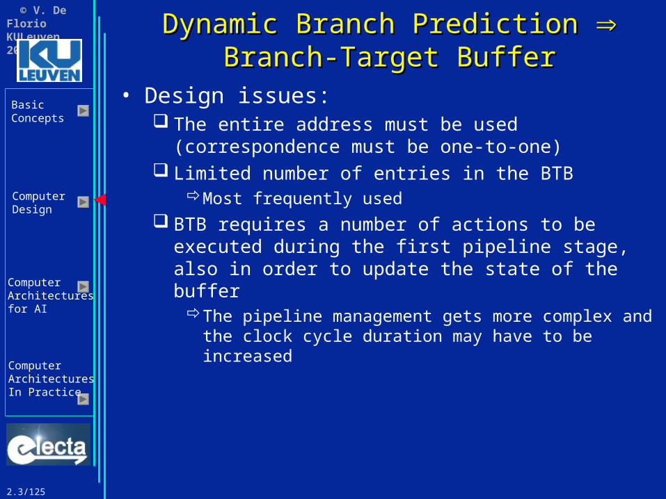
• Design issues: The entire address must be used (correspondence
must be one-to-one) Limited number of entries in the BTB
Most frequently used BTB requires a number of actions to be executed
during the first pipeline stage, also in order to update the state of the buffer
The pipeline management gets more complex and the clock cycle duration may have to be increased

2.3/126
© V. De FlorioKULeuven 2002
BasicConcepts
ComputerDesign
ComputerArchitecturesfor AI
ComputerArchitecturesIn Practice
Dynamic Branch Prediction Dynamic Branch Prediction Branch-Target BufferBranch-Target Buffer
• Total branch penalty for a BTB• Assumptions: penalties are as follows
Instruction Prediction Actual Penaltyis in buffer branch cycles
Yes Taken Taken 0
Yes Taken Untaken 2
No * Taken 2
• Prediction accuracy: 90%• Hit rate in buffer: 90%• Taken branch frequency: 60%

2.3/127
© V. De FlorioKULeuven 2002
BasicConcepts
ComputerDesign
ComputerArchitecturesfor AI
ComputerArchitecturesIn Practice
Dynamic Branch Prediction Dynamic Branch Prediction Branch-Target BufferBranch-Target Buffer
• Branch penalty =Percent buffer hit rate xPercent incorrect predictions xPenalty
+ (1 - Percent buffer hit rate) xPercent taken branches xPenalty =
Instruction Prediction Actual Penaltyis in buffer branch cycles
Yes Taken Taken 0
Yes Taken Untaken 2
No * Taken 2
10%
90%10%
60%
90%x10%x2 + 10%x60%x2 = 0.18+0.12=0.30 clock cycles (vs. 0.50 for delayed br.)

2.3/128
© V. De FlorioKULeuven 2002
BasicConcepts
ComputerDesign
ComputerArchitecturesfor AI
ComputerArchitecturesIn Practice
Dynamic Branch Prediction Dynamic Branch Prediction Branch-Target BufferBranch-Target Buffer
• The same approach can be applied to the procedures return addresses
• Example:0x4ABC CALL 0x30A00x4AC0 ……0x4CF4 CALL 0x30A00x4CF8 ……
0x30A0 0x4CF8
0x4AC0
• Associative arrays of stacks• If cache is large enough, all return addresses
are predicted correctly

2.3/129
© V. De FlorioKULeuven 2002
BasicConcepts
ComputerDesign
ComputerArchitecturesfor AI
ComputerArchitecturesIn Practice
ParallelismParallelism
• Introduction to parallel processing• Instruction level parallelism
Introduction VLIW Advanced pipelining techniques Superscalar

2.3/130
© V. De FlorioKULeuven 2002
BasicConcepts
ComputerDesign
ComputerArchitecturesfor AI
ComputerArchitecturesIn Practice
Superscalar architecturesSuperscalar architectures
• So far, the goal was reaching the ideal CPI = 1 goal
• Further increasing performance by having CPI < 1 is the goal of superscalar processors (SP)
• To reach this goal, SP issue multiple instructions in the same clock cycle
• Multiple-issue processors VLIW (seen already) SP
Statically scheduled (compiler)Dynamically scheduled (HW;
Scoreboarding/Tomasulo)
• In SP, a varying # of instructions is issued, depending on structural limits and dependencies

2.3/131
© V. De FlorioKULeuven 2002
BasicConcepts
ComputerDesign
ComputerArchitecturesfor AI
ComputerArchitecturesIn Practice
Superscalar architecturesSuperscalar architectures
• Superscalar version of DLX• At most two instructions per clock cycle can
be issued1. One of: load, store (integer or FP), branch, integer
ALU operation2. A FP ALU operation
• IF and ID operate on 64 bits of instructions• Multiple independent FPU are available

2.3/132
© V. De FlorioKULeuven 2002
BasicConcepts
ComputerDesign
ComputerArchitecturesfor AI
ComputerArchitecturesIn Practice
Superscalar architecturesSuperscalar architectures
• The superscalar DLX is indeed a sort of “bidimensional pipeline”:
IFInteger Instr. EXID WBMEMIFFP Instr. EXID WBMEM
IF EXID WBMEMIF EXID WBMEM
Integer Instr.FP Instr.Integer Instr.FP Instr.Integer Instr.FP Instr.
IF EXID WBMEMIF EXID WBMEM
IF EXID WBMEMIF EXID WBMEM

2.3/133
© V. De FlorioKULeuven 2002
BasicConcepts
ComputerDesign
ComputerArchitecturesfor AI
ComputerArchitecturesIn Practice
Superscalar architecturesSuperscalar architectures
• Every new solution breeds new problems..• Latencies!• When the latency of the load is 1:
In the “monodimensional pipeline”, one cannot use the result of the load in the current and next cycle:
PLD NOP LDc
In the bidimensional pipeline of SP, this means a loss of three cycles:
Pi
LD NOP
LDcNOPNOP
LDc’
Pfp

2.3/134
© V. De FlorioKULeuven 2002
BasicConcepts
ComputerDesign
ComputerArchitecturesfor AI
ComputerArchitecturesIn Practice
Superscalar architecturesSuperscalar architectures
• Let us consider again the following loop:Loop: LD F0, 0(R1) ADDD F4, F0, F2 SD 0(R1), F4 SUBI R1, R1, #8 BNEZ R1, Loop
• Let us perform unrolling (x5) + scheduling on the Superscalar DLX:

2.3/135
© V. De FlorioKULeuven 2002
BasicConcepts
ComputerDesign
ComputerArchitecturesfor AI
ComputerArchitecturesIn Practice
Superscalar architecturesSuperscalar architectures
Integer FP Cycle
Loop: LD F0, 0(R1) 1
LD F6, -8(R1) 2
LD F10, -16(R1)ADDD F4,F0,F2 3
LD F14, -24(R1)ADDD F8,F6,F2 4
LD F18, -32(R1)ADDD F12,F10,F2 5
SD 0(R1), F4 ADDD F16,F14,F2 6
SD -8(R1), F8 ADDD F20,F18,F2 7
SD -16(R1), F12 8
SD -24(R1), F16 9
SUBI R1, R1, #40 10
BNEZ R1, Loop 11
SD -32(R1), F20 12
• 12 clock cycles per 5 iterations = 2.4 cc/i

2.3/136
© V. De FlorioKULeuven 2002
BasicConcepts
ComputerDesign
ComputerArchitecturesfor AI
ComputerArchitecturesIn Practice
Superscalar architecturesSuperscalar architectures
• Superscalar = 2.4 cc/i vs normal = 3.5 cc/i• But in the example there were not enough FP
instructions to keep the FP pipeline in use From cycle 8 to cycle 12 and for the first two
cycles, each cycle holds just one instruction
• How to get more?
Dynamic scheduling for SP Multicycle extension of the Tomasulo algorithm

2.3/137
© V. De FlorioKULeuven 2002
BasicConcepts
ComputerDesign
ComputerArchitecturesfor AI
ComputerArchitecturesIn Practice
Superscalar architectures and the Superscalar architectures and the Tomasulo algorithmTomasulo algorithm
• Idea: employing separate data structures for the Integer and the FP registers Integer Reservation Stations (IRS) FP Reservation Stations (FRS)
• In the same cycle, issue a FP (to a FRS) and an integer instruction (to a IRS)
• Note: issuing does not mean executing! Possible dependencies might serialize the two
instructions issued in parallel
• Dual issue is obtained pipelining the instruction-issue stageso that it runs twice as fast

2.3/138
© V. De FlorioKULeuven 2002
BasicConcepts
ComputerDesign
ComputerArchitecturesfor AI
ComputerArchitecturesIn Practice
Superscalar architecturesSuperscalar architectures
• Multiple issue strategy’s inherent limitations: The amount of ILP may be limited (see loop p.134)
Extra HW is requiredMultiple FPU and IUMore complex (-> slower) design
Extra need for large memory and register-file bandwith
Increase in code size due to hard loop unrolling
Recall: CPUTIME(p) = IC(p) CPI(p) clock rate

2.3/139
© V. De FlorioKULeuven 2002
BasicConcepts
ComputerDesign
ComputerArchitecturesfor AI
ComputerArchitecturesIn Practice
Superscalar architectures: compiler Superscalar architectures: compiler supportsupport
• Symbolic loop unrolling The loop is not physically unrolled, though
reorganized, so to eliminate dependencies
• Software pipelining: Dependencies are eliminated by interleaving
instructions from different iterations of the loop Loop is not unrolled
Loop: LD F0, 0(R1) ADDD F4, F0, F2 SD 0(R1), F4 SUBI R1, R1, #8 BNEZ R1, Loop
<startup>
Loop: SD 0(R1), F4 ADDD F4, F0, F2 LD F0, -16(R1) SUBI R1, R1, #8 BNEZ R1, Loop<clean-up>
RAW: problematic WAR: HW removable
2.3/140
© V. De FlorioKULeuven 2002
BasicConcepts
ComputerDesign
ComputerArchitecturesfor AI
ComputerArchitecturesIn Practice
Superscalar architectures: compiler Superscalar architectures: compiler supportsupport
• Trace scheduling• Aim: tackling the problem of too short basic
blocks• Method:
Trace selection Trace compaction

2.3/141
© V. De FlorioKULeuven 2002
BasicConcepts
ComputerDesign
ComputerArchitecturesfor AI
ComputerArchitecturesIn Practice
Superscalar architectures: compiler Superscalar architectures: compiler supportsupport
• Trace selection: A number of contiguous basic blocks are put
together into a “trace” Using static branch prediction, the conditional
branches are chosen as taken/untaken, while loop branches are considered as taken
A
B
C
Book-keeping
A
B X
C
test

2.3/142
© V. De FlorioKULeuven 2002
BasicConcepts
ComputerDesign
ComputerArchitecturesfor AI
ComputerArchitecturesIn Practice
Superscalar architectures: compiler Superscalar architectures: compiler supportsupport
• Trace compaction: The resulting trace is a longer straight-line of code Trace compaction: global code scheduling
A
B
C
Book-keeping
Code scheduling witha basic block whose sizeis that of A + B + C
• Speculative movement of code

2.3/143
© V. De FlorioKULeuven 2002
BasicConcepts
ComputerDesign
ComputerArchitecturesfor AI
ComputerArchitecturesIn Practice
Superscalar architectures: Superscalar architectures: HW supportHW support
• Conditional instructions: instructions likeCMOVZ R2, R3, R1
which meansif (R1 == 0) R2 = R3;
or (R1)? R2 = R3 : /* NOP */;• The instruction turns into a NOP if the
condition is not met This also means that no exception are raised!
• Using conditional instructions we convert a control dependence (due to a branch) into a data dependence
• Speculative transformation in a two-issue superscalar with conditional instructions:

2.3/144
© V. De FlorioKULeuven 2002
BasicConcepts
ComputerDesign
ComputerArchitecturesfor AI
ComputerArchitecturesIn Practice
Superscalar architectures: HW support Superscalar architectures: HW support : conditional instructions: conditional instructions
Integer FP Cycle
LW R1, 40(R2) ADDD R3,R4,R51
ADDD R6,R3,R72
BEQZ R10, L 3
LW R8, 20(R10) 4
LW R9,0(R8) 5
LW R1, 40(R2) ADDD R3,R4,R51
LWC R8,20(R10),R10 ADDD R6,R3,R72
BEQZ R10, L 3
LW R9,0(R8) 4
We speculate on the outcome of the branch. If the condition is not met, we don’t slow down the execution,because we had used a slot that would otherwise be lost

2.3/145
© V. De FlorioKULeuven 2002
BasicConcepts
ComputerDesign
ComputerArchitecturesfor AI
ComputerArchitecturesIn Practice
Superscalar architectures: HW support Superscalar architectures: HW support : conditional instructions: conditional instructions
• Conditional instructions are useful to implement short alternative control flows
• Their usefulness though is limited by several factors: Conditional instructions that are annullated still
take execution time – unless they are scheduled into waste slots
They are good only in limited cases, when there’s a simple alternative sequence
Moving an instruction across multiple branches would require double-conditional instructions!
LWCC R1, R2, R10, R12(makes no sense)
They require to do extra work w.r.t. their “regular” version
The extra time required for the test may require more cycles than the regular versions

2.3/146
© V. De FlorioKULeuven 2002
BasicConcepts
ComputerDesign
ComputerArchitecturesfor AI
ComputerArchitecturesIn Practice
Superscalar architectures: HW support Superscalar architectures: HW support : conditional instructions: conditional instructions
• Most architectures support a few conditional instructions (conditional move)
• The HP PA architecture allows any register-register instruction to turn the next instruction into a NOP – which makes that a conditional instruction
• Exceptions

2.3/147
© V. De FlorioKULeuven 2002
BasicConcepts
ComputerDesign
ComputerArchitecturesfor AI
ComputerArchitecturesIn Practice
Superscalar architectures: HW support Superscalar architectures: HW support : conditional instructions: conditional instructions
• Exceptions: Fatal (normally causing termination; e.g., memory
protection violation) Resumable exceptions (causing a delay, but no
termination; e.g., page fault exception)
• Resumable exceptions can be processed for speculative instructions just as if they were normal instructions Corresponding time penalty is not considered as
incorrect
• Fatal exceptions cannot be handled by speculative instructions, hence must be deferred to the next non-speculative instructions

2.3/148
© V. De FlorioKULeuven 2002
BasicConcepts
ComputerDesign
ComputerArchitecturesfor AI
ComputerArchitecturesIn Practice
Superscalar architectures: HW support Superscalar architectures: HW support : conditional instructions: conditional instructions
• Moving instructions across a branch must not affect The (fatal) exception behaviour The data dependences
• How to obtain this?1. All the exceptions triggered by speculative
instructions are ignored by HW and OS
The HW and OS do handle all exceptions, but return an undefined value for any fatal exception. The program is allowed to continue – though this will almost certainly lead to incorrect results
Note: scheme 1. can never cause a correct program to fail, regardless the fact that you used or not speculation

2.3/149
© V. De FlorioKULeuven 2002
BasicConcepts
ComputerDesign
ComputerArchitecturesfor AI
ComputerArchitecturesIn Practice
Superscalar architectures: HW support Superscalar architectures: HW support : conditional instructions: conditional instructions
2. Poison bits: A speculative instructions does not trigger any exception, but turns a bit on in the involved result registers. Next “normal” (non-speculative) instruction using those registers will be “poisoned” -> it will cause an exception
3. Boosting: Renaming and buffering in the HW (similar to the Tomasulo approach)
• Speculation can be used, e.g., to optimize an if-the-else such as
if (a==0) a = b; else a = a + 4
or, equivalently,
a = (a==0)? b : a + 4

2.3/150
© V. De FlorioKULeuven 2002
BasicConcepts
ComputerDesign
ComputerArchitecturesfor AI
ComputerArchitecturesIn Practice
Superscalar architectures: HW support Superscalar architectures: HW support : conditional instructions: conditional instructions
• Suppose A is in 0(R3) and B in 0(R2)• Example:
LW R1, 0(R3) ; load ABNEZ R1, L1 ; A != 0 ? GOTO L1LW R1, 0(R2) ; load BJ L2 ; skip ELSE
L1:ADD R1,R1,4 ; ELSE partL2:SW 0(R3), R1 ; store A
• Speculation:LW R1, 0(R3) ; load ALW R9, 0(R2) ; load speculatively BBNEZ R1, L3ADD R9, R1, 4 ; here R9 is A+4
L3: SW 0(R3), R9 ; here R9 is A+4 or B• In this case, a temporary register is used• Method 1: speculation is transparent

2.3/151
© V. De FlorioKULeuven 2002
BasicConcepts
ComputerDesign
ComputerArchitecturesfor AI
ComputerArchitecturesIn Practice
Superscalar architectures: HW support Superscalar architectures: HW support : conditional instructions: conditional instructions
• Method 2 applied to the previous code fragment:
LW R1, 0(R3) ; load ALW* R9, 0(R2) ; load speculatively BBNEZ R1, L3ADD R9, R1, 4 ; here R9 is A+4
L3: SW 0(R3), R9 ; here R9 is A+4 or B• LW* is a speculative version of LW• LW* an opcode that turns on the poison bit of
register R9• Next non speculative instruction using R9 will
be “poisoned”: it will cause an exception• If another speculative instruction uses R9, the
poison bit will be inherited
2.3/152
© V. De FlorioKULeuven 2002
BasicConcepts
ComputerDesign
ComputerArchitecturesfor AI
ComputerArchitecturesIn Practice
Superscalar architectures: HW support Superscalar architectures: HW support : conditional instructions: conditional instructions
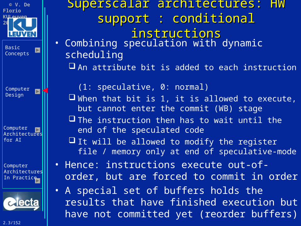
• Combining speculation with dynamic scheduling An attribute bit is added to each instruction
(1: speculative, 0: normal) When that bit is 1, it is allowed to execute, but
cannot enter the commit (WB) stage The instruction then has to wait until the end of the
speculated code It will be allowed to modify the register file /
memory only at end of speculative-mode
• Hence: instructions execute out-of-order, but are forced to commit in order
• A special set of buffers holds the results that have finished execution but have not committed yet (reorder buffers)

2.3/153
© V. De FlorioKULeuven 2002
BasicConcepts
ComputerDesign
ComputerArchitecturesfor AI
ComputerArchitecturesIn Practice
Superscalar architectures: HW support Superscalar architectures: HW support : conditional instructions: conditional instructions
• As neither the register values nor the memory values are actually WRITTEN until an instruction commits,the processor can easily undo its speculative actions when a branch is found to be mispredicted
• If a speculated instruction raises an exception, this is recorded in the reorder buffer
• In case of branch misprediction such that a certain speculative instruction should not have been executed, the exception is flushed along with the instruction when the reorder buffer is cleared

2.3/154
© V. De FlorioKULeuven 2002
BasicConcepts
ComputerDesign
ComputerArchitecturesfor AI
ComputerArchitecturesIn Practice
Superscalar architectures: HW support Superscalar architectures: HW support : conditional instructions: conditional instructions
• Reorder buffers: An additional set of virtual registers that hold the
result of the instructionsThat have finished execution, butHave not committed yet
Issue: only when both a Reservation Station and a reorder buffer are available
As soon as an instruction completes, its output goes into its reorder buffer
Until the instruction has not committed, input is received from the reorder buffer(the Reservation Station is freed, the reorder buffer is not)
The actual updating of registers takes place when the instruction reaches the top of the list of reorder buffers

2.3/155
© V. De FlorioKULeuven 2002
BasicConcepts
ComputerDesign
ComputerArchitecturesfor AI
ComputerArchitecturesIn Practice
Superscalar architectures: HW support Superscalar architectures: HW support : conditional instructions: conditional instructions
• At this point the commit phase takes place: Either the result is written into the register file, Or, in case of a mispredicted branch, the reorder
buffer is flushed and execution restarts at the correct successor of the branch
• Assumption: when a branch with incorrect prediction reaches the head of the buffer, it means that the speculation was wrong

2.3/156
© V. De FlorioKULeuven 2002
BasicConcepts
ComputerDesign
ComputerArchitecturesfor AI
ComputerArchitecturesIn Practice
Superscalar architectures: HW support Superscalar architectures: HW support : conditional instructions: conditional instructions
• This technique allows also to tackle situation likeif (cond) do_this ; else do_that ;
• One may “bet” on the outcome of the branch and say, e.g., it will be a taken one
• Even unlikely events do happen, so sooner or later a misprediction occurs
• Idea: let the instructions in the else part (do_that) issue and execute, with a separate list of reorder buffers (list2)
• This second list is simpler: we don’t check for the current head-of-list. Elements in there need to be explicitly removed
• In case of a misprediction, in the second list we have already executed the do_that part, and we just need to perform its commit
• In case of positive prediction, the ELSE part is purged off list2

2.3/157
© V. De FlorioKULeuven 2002
BasicConcepts
ComputerDesign
ComputerArchitecturesfor AI
ComputerArchitecturesIn Practice
Superscalar architecturesSuperscalar architectures
• If a processor A has a lower CPI w.r.t another processor B, will A always run faster than B?
• Not always! A higher clock rate is indeed a deterministic
measure of the performance improvement A multiple issue (superscalar) architecture cannot
guarantee its improvements (stochastic improvements)
Pushing towards a low CPI means adapting sophisticated (=complex) techniques… which slows down the clock rate!
Improving one aspect of a M.I.P. does not necessarily lead to overall performance improvements

2.3/158
© V. De FlorioKULeuven 2002
BasicConcepts
ComputerDesign
ComputerArchitecturesfor AI
ComputerArchitecturesIn Practice
Superscalar architecturesSuperscalar architectures
• A simple question:“how much ILP exists in a program?”or, in other words, “how much can we expect from techniques that are based on the exploitation of the ILP?”
• How to proceed: Delivering a set of very optimistic assumptions and
measuring how much parallelism is available under those assumptions

2.3/159
© V. De FlorioKULeuven 2002
BasicConcepts
ComputerDesign
ComputerArchitecturesfor AI
ComputerArchitecturesIn Practice
Superscalar architecturesSuperscalar architectures
• Assumptions (HW model of an ideal processor):1. Infinite # of virtual registers (-> no WAW or WAR
can suspend the pipeline)2. All conditional branches are predicted exactly (!!)3. All computed jumps and returns are perfectly
predicted4. All memory addresses are known exactly, so a
store can be moved before a load – provided that the addresses are not identical
5. Infinite issue processor6. No restriction about the types of instructions to be
executed in a cycle (no structural hazards)7. All latencies are 1

2.3/160
© V. De FlorioKULeuven 2002
BasicConcepts
ComputerDesign
ComputerArchitecturesfor AI
ComputerArchitecturesIn Practice
Superscalar architecturesSuperscalar architectures
• How to match these assumptions??• Gambling!• We run a program and produce a trace with
all the values of all the instances of each branch Taken, Taken, Taken, Untaken, Taken, … Each corresponding target address is recorded and
assumed to be available Then we use a simulator to mimic, e.g., an infinite
virtual registers machine etc.
• Results are depicted in next picture• Parallelism is expressed in IPC: instruction
issues per clock cycles

2.3/161
© V. De FlorioKULeuven 2002
BasicConcepts
ComputerDesign
ComputerArchitecturesfor AI
ComputerArchitecturesIn Practice
Superscalar architecturesSuperscalar architectures
• Tomcatv reaches 150 IPC (for a particular run)
g c c
e s p re s s o
liS P E C b e n c h m a rk s
fp p p p
d o d u c
to m c a tv
5 4 .8
6 2 .6
1 7 .9
7 5 .2
11 8 .7
1 5 0 .1
1 4 0 1 6 0

2.3/162
© V. De FlorioKULeuven 2002
BasicConcepts
ComputerDesign
ComputerArchitecturesfor AI
ComputerArchitecturesIn Practice
Superscalar architecturesSuperscalar architectures
• Then we can diminish the above assumptions and introduce limitations that represent our current possibilities with computer design techniques for ILP Window size: the actual range of instructions we
inspect when looking for candidates for contemporary issuing
Realistic branch prediction Finite # of registers
• See images 4-39 and 4-40

2.3/163
© V. De FlorioKULeuven 2002
BasicConcepts
ComputerDesign
ComputerArchitecturesfor AI
ComputerArchitecturesIn Practice
Superscalar architecturesSuperscalar architectures
1 6 0
1 4 0
1 2 0
1 0 0
In s tru c tio n is s u e s p e r c y c le
8 0
6 0
4 0
2 0
0 In f in ite 2 k 5 1 2 1 2 8
W in d o w s iz e
g c c
fp p p p
e s p re s s o
d o d u c
li
to m c a tv
3 2 8 4

2.3/164
© V. De FlorioKULeuven 2002
BasicConcepts
ComputerDesign
ComputerArchitecturesfor AI
ComputerArchitecturesIn Practice
Superscalar architecturesSuperscalar architectures
g c c
e s p re s s o
li
fp p p p
B e n c h m a rk s
d o d u c
to m c a tv
0
5 51 01 0
84
3
1 51 3
84
3
1 81 211
94
3
4 97 5
6 3
11 9
3 51 4
53
1 61 5
94
3
1 5 04 5
3 41 4
63
2 0
In fin ite
8
5 1 2 1 2 8 3 2
4
4 0 6 0 8 0
In s tru c tio n is s u e s p e r c y c le
1 0 0 1 2 0 1 4 0 1 6 0

2.3/165
© V. De FlorioKULeuven 2002
BasicConcepts
ComputerDesign
ComputerArchitecturesfor AI
ComputerArchitecturesIn Practice
Superscalar architectures: conclusive Superscalar architectures: conclusive notesnotes
• In the next 10 years it is realistic to reach an architecture that looks like this: 64 instruction issues per clock cycle Selective predictor, 1K entries, 16-entry return
predictor Perfect disambiguation of memory references Register renaming with 64 + 64 extra registers
• Computer architectures in practice: Section 4.8 (PowerPC 620)

2.3/166
© V. De FlorioKULeuven 2002
BasicConcepts
ComputerDesign
ComputerArchitecturesfor AI
ComputerArchitecturesIn Practice
Superscalar architectures: conclusive Superscalar architectures: conclusive notesnotes
6 0
5 0
4 0
3 0
2 0
1 0
0In fin ite
Instruction
issues pe
r cycle
2 5 6 1 2 8
W in d o w s iz e
3 2 1 6 86 4 4
g c c
fp p p p
e s p re s s o
d o d u c
li
to m c a tv
• Reachable performance

2.3/167
© V. De FlorioKULeuven 2002
BasicConcepts
ComputerDesign
ComputerArchitecturesfor AI
ComputerArchitecturesIn Practice
Pipelining and communicationsPipelining and communications
• Suppose that N+1 processes need to communicate a private value to all the others
• They use all the values to produce next output (e.g., for voting)
• Communication is fully synchronous and needs to be repeated m times, m large
. . .

2.3/168
© V. De FlorioKULeuven 2002
BasicConcepts
ComputerDesign
ComputerArchitecturesfor AI
ComputerArchitecturesIn Practice
Pipelining and communicationsPipelining and communications
• Let us assume that no bus is available • Point-to-point communication
• Processes are numbered p0…pN
• Two instructions are available Send (pj, value)
Receive (pj, &value)
• Blocking functions• If the receiver is ready to receive, they last
one stage time, otherwise they block the caller for a multiple of the stage time
• Sending and receiving occur at discrete time steps

2.3/169
© V. De FlorioKULeuven 2002
BasicConcepts
ComputerDesign
ComputerArchitecturesfor AI
ComputerArchitecturesIn Practice
Pipelining and communicationsPipelining and communications
• In each time t, processor pi may be Sending data (next stage pi is unblocked)
Receiving data (next stage pi is unblocked)
Blocked in a Receive() Blocked in a Send()
• Slot = time corresponding to an entire stage time
• Each time t we have n slots (a slot per process)
• If pi is blocked, its slot is wasted (it’s a “bubble”)
• Otherwise the slot is used

2.3/170
© V. De FlorioKULeuven 2002
BasicConcepts
ComputerDesign
ComputerArchitecturesfor AI
ComputerArchitecturesIn Practice
Pipelining and communicationsPipelining and communications
• In each time t, processor pi may be in State S(j) : Sending data to processor pj
State R(j) : Receiving data from pj
State WR(j) : Blocked in a Receive( pj, … )
State WS(j) : Blocked in a Send( pj, …)
• We use formalism:proc st proc’
to indicate that, at time t, proc is in state s with proc’
• For instance
p1 WR(4)21 p3
means that the 21st slot of p1 is wasted waiting for p3 to send its value to it

2.3/171
© V. De FlorioKULeuven 2002
BasicConcepts
ComputerDesign
ComputerArchitecturesfor AI
ComputerArchitecturesIn Practice
Pipelining and communicationsPipelining and communications
• The following algorithm is executed by process j:
Before gaining the right to broadcast, process j needs to go through j couples of states (WR, R)
Ordered broadcast : the k-th message to be sent goes to
process pk
Finally, process j goes through N-j couples of states (WR, R)

2.3/172
© V. De FlorioKULeuven 2002
BasicConcepts
ComputerDesign
ComputerArchitecturesfor AI
ComputerArchitecturesIn Practice
Pipelining and communicationsPipelining and communications
• p is a vector of indices
• For process j, p can be any arrangement of the integers 0, 1, …, j-1, j+1, … N
• Whatever the arrangement, the algorithm works correctly
• For instance, if N = 4 (5 processes) and j = 1, then p can be any permutation of0, 2, 3, and 4
• p determines the order in which process j sends its value to its neighbours
• Example: p[] = [ 3, 2, 0, 4]. Then p1 executes:send (p3), send(p2), send(p0), send(p4)

2.3/173
© V. De FlorioKULeuven 2002
BasicConcepts
ComputerDesign
ComputerArchitecturesfor AI
ComputerArchitecturesIn Practice
Pipelining and communicationsPipelining and communications
• Example: p[] = ordered permutation Ex: N=5 and pj p [ 0, … j-1,j+1, … N ]
Frequencies of used slots Slot wasted in send
Slot wasted in receive
Duration

2.3/174
© V. De FlorioKULeuven 2002
BasicConcepts
ComputerDesign
ComputerArchitecturesfor AI
ComputerArchitecturesIn Practice
Pipelining and communicationsPipelining and communications
• Case N = 20, p[] = ordered permutation
• Gray = wasted slots• Black = used slots
• In general, duration is
• Used slots / total # of slots
• Average # used slots during one stage time
• This image: reminds us of another one:

2.3/175
© V. De FlorioKULeuven 2002
BasicConcepts
ComputerDesign
ComputerArchitecturesfor AI
ComputerArchitecturesIn Practice
No pipelining: Many slots are wasted!
30
B
C
D
A
Time
3030 3030 30 3030 3030 3030 3030 3030
6 PM 7 8 9 10 11 12 1 2 AM
Pipelining and communicationsPipelining and communications

2.3/176
© V. De FlorioKULeuven 2002
BasicConcepts
ComputerDesign
ComputerArchitecturesfor AI
ComputerArchitecturesIn Practice
Pipelining and communicationsPipelining and communications
• Let us now consider the case in which processor k uses
p[] = [ k+1, k+2, …, N, O, 1, …, k-1 ]

2.3/177
© V. De FlorioKULeuven 2002
BasicConcepts
ComputerDesign
ComputerArchitecturesfor AI
ComputerArchitecturesIn Practice
Pipelining and communicationsPipelining and communications

2.3/178
© V. De FlorioKULeuven 2002
BasicConcepts
ComputerDesign
ComputerArchitecturesfor AI
ComputerArchitecturesIn Practice
Pipelining and communicationsPipelining and communications
• Duration: first case vs. second case

2.3/179
© V. De FlorioKULeuven 2002
BasicConcepts
ComputerDesign
ComputerArchitecturesfor AI
ComputerArchitecturesIn Practice
Pipelining and communicationsPipelining and communications
• Efficiency: first case vs. second case
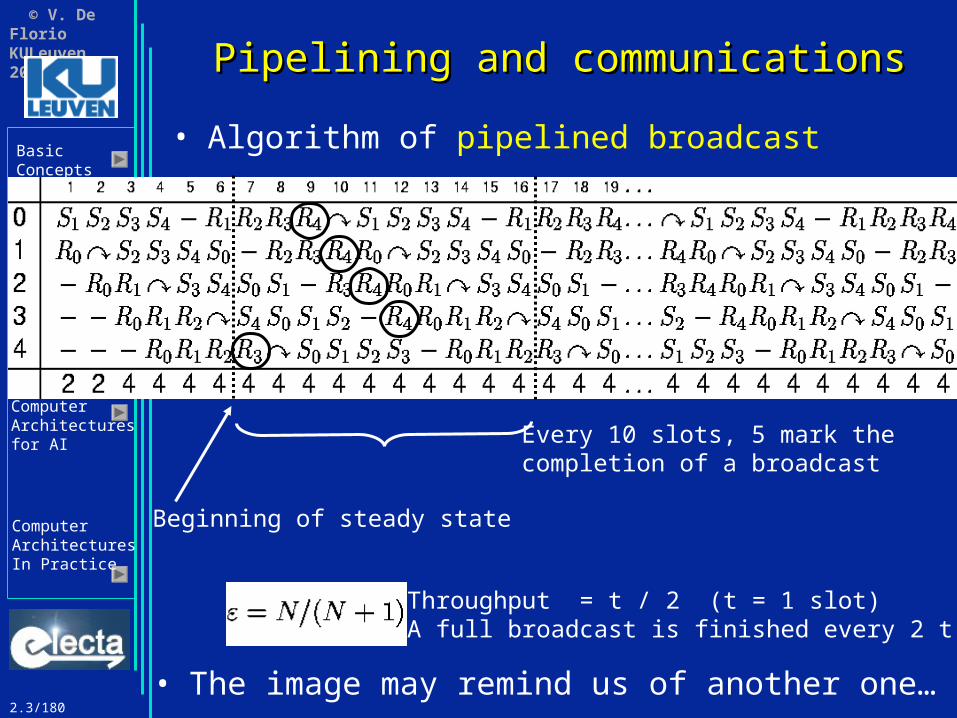
2.3/180
© V. De FlorioKULeuven 2002
BasicConcepts
ComputerDesign
ComputerArchitecturesfor AI
ComputerArchitecturesIn Practice
Pipelining and communicationsPipelining and communications
• Algorithm of pipelined broadcast
Beginning of steady state
Every 10 slots, 5 mark the completion of a broadcast
Throughput = t / 2 (t = 1 slot)A full broadcast is finished every 2 t
• The image may remind us of another one…

2.3/181
© V. De FlorioKULeuven 2002
BasicConcepts
ComputerDesign
ComputerArchitecturesfor AI
ComputerArchitecturesIn Practice
Between 7.30 and 9.30pm, a whole job is completed every 30’
6 PM
B
C
D
A
303030 3030
Pipelining (slide P2.2/20)Pipelining (slide P2.2/20)
…
…
…
…
During that period, each worker is permanently at work…
…but a new input must arrive within 30’
12 2 AM7 8 9 10 11 1