© The McGraw-Hill Companies, Inc., 2004 1 Chapter 14 Inventory Control.
47
©The McGraw-Hill Companies, Inc., 2004 1 Chapter 14 Inventory Control
-
date post
20-Dec-2015 -
Category
Documents
-
view
218 -
download
0
Transcript of © The McGraw-Hill Companies, Inc., 2004 1 Chapter 14 Inventory Control.

©The McGraw-Hill Companies, Inc., 2004
1
Chapter 14
Inventory Control

©The McGraw-Hill Companies, Inc., 2004
2
• Definition and Purpose of Inventory
• Inventory Costs
• Independent vs. Dependent Demand
• Single-Period Inventory Model
• Multi-Period Inventory Models: Basic Fixed-Order Quantity Models
• Multi-Period Inventory Models: Basic Fixed-Time Period Model
• Miscellaneous Systems and Issues
OBJECTIVES

©The McGraw-Hill Companies, Inc., 2004
3
Inventory SystemDefined
• Inventory is the stock of any item or resource used in an organization. They are carried in anticipation of use and can include:— raw materials— finished products— component parts— supplies, and— work-in-process
• An inventory system is the set of policies and controls that monitor levels of inventory and determines what levels should be maintained, when stock should be replenished, and how large orders should be

©The McGraw-Hill Companies, Inc., 2004
4
Problems of Inventory Management
• When to order the products— Issue of timing
• How much to order— Issue of quantity
• These problems often addressed with the objective of inventory cost minimization— Total annual cost— And meet prescribed service levels

©The McGraw-Hill Companies, Inc., 2004
5
Purposes of Inventory
1. To maintain independence of operations
2. To meet variation in product demand
3. To allow flexibility in production scheduling
4. To provide a safeguard for variation in raw material delivery time
5. To take advantage of economic purchase-order size

©The McGraw-Hill Companies, Inc., 2004
6
Wrong Reasons for Carrying Inventory
• Poor quality
• Inadequate maintenance of machines
• Poor production schedules
• Unreliable suppliers
• Poor worker’s attitudes
• Just-in-case

©The McGraw-Hill Companies, Inc., 2004
7
Inventory Costs
• Holding (or carrying) costs: H— Costs for physical storage space— Handling— Taxes and insurance, etc.— Breakage, spoilage, deterioration,
obsolescence— Cost of capital
• Setup (or production change) costs: S— Costs for arranging specific equipment setups,
etc.
©The McGraw-Hill Companies, Inc., 2004
8
Inventory Costs: Continued
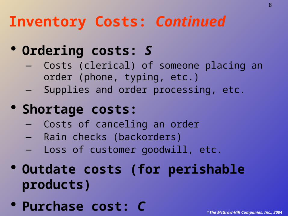
Ordering costs: S— Costs (clerical) of someone placing an order (phone,
typing, etc.)— Supplies and order processing, etc.
Shortage costs:— Costs of canceling an order— Rain checks (backorders)— Loss of customer goodwill, etc.
Outdate costs (for perishable products)
Purchase cost: C

©The McGraw-Hill Companies, Inc., 2004
9
E(1)
Independent vs. Dependent Demand
Independent Demand (Demand for the final end-product or demand not related to other items)
Dependent Demand
(Derived demand items for
component parts, subassemblies,
raw materials, etc)
Finishedproduct
Component parts

©The McGraw-Hill Companies, Inc., 2004
10
Classification of Inventory Systems:Single Period Models
• Single-Period Inventory Model
— One time purchasing decision: Example:
Vendor selling T-shirts at a football game Newspaper sales (Newsboy Model)
— Seeks to balance the costs of inventory overstock and under stock

©The McGraw-Hill Companies, Inc., 2004
11
Classifying Inventory Models:Multi-Period Models
• Fixed-Order Quantity Models— Event triggered (Example: running out of stock)— Inventory is monitored all the time— Order Q when inventory reaches R, the reorder point— Also known as FOSS, (Q,R) or EOQ system
• Fixed-Time Period Models — Time triggered (Example: Monthly sales call by sales
representative)— Inventory is monitored periodically— Also known as FOIS, (S,S), or EOI system
©The McGraw-Hill Companies, Inc., 2004
12
Single-Period Inventory Model
uo
u
CC
CP
uo
u
CC
CP
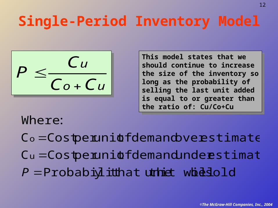
sold be unit will y that theProbabilit
estimatedunder demand ofunit per Cost C
estimatedover demand ofunit per Cost C
:Where
u
o
P
This model states that we should continue to increase the size of the inventory so long as the probability of selling the last unit added is equal to or greater than the ratio of: Cu/Co+Cu
This model states that we should continue to increase the size of the inventory so long as the probability of selling the last unit added is equal to or greater than the ratio of: Cu/Co+Cu

©The McGraw-Hill Companies, Inc., 2004
13
Single Period Model Example
• Our college basketball team is playing in a tournament game this weekend. Based on our past experience we sell on average 2,400 shirts with a standard deviation of 350. We make $10 on every shirt we sell at the game, but lose $5 on every shirt not sold. How many shirts should we make for the game?
Cu = $10 and Co = $5; P ≤ $10 / ($10 + $5) = .667
Z.667 = .432 (use NORMSDIST(.667) or Appendix E)
therefore we need 2,400 + .432(350) = 2,551 shirts

©The McGraw-Hill Companies, Inc., 2004
14
Multi-Period Models:Fixed-Order Quantity Model Model
Assumptions (Part 1)
• Demand for the product is constant and uniform throughout the period
• Lead time (time from ordering to receipt) is constant
• Price per unit of product is constant

©The McGraw-Hill Companies, Inc., 2004
15
Multi-Period Models:Fixed-Order Quantity Model Model
Assumptions (Part 2)
• Inventory holding cost is based on average inventory
• Ordering or setup costs are constant
• All demands for the product will be satisfied (No back orders are allowed)

©The McGraw-Hill Companies, Inc., 2004
16
Basic Fixed-Order Quantity Model and Reorder Point Behavior
R = Reorder pointQ = Economic order quantityL = Lead time
L L
Q QQ
R
Time
Numberof unitson hand
1. You receive an order quantity Q.
2. Your start using them up over time. 3. When you reach down to a
level of inventory of R, you place your next Q sized order.
4. The cycle then repeats.

©The McGraw-Hill Companies, Inc., 2004
17
Cost Minimization Goal
Ordering Costs
HoldingCosts
Order Quantity (Q)
COST
Annual Cost ofItems (DC)
Total Cost
QOPT
By adding the item, holding, and ordering costs together, we determine the total cost curve, which in turn is used to find the Qopt inventory order point that minimizes total costs
By adding the item, holding, and ordering costs together, we determine the total cost curve, which in turn is used to find the Qopt inventory order point that minimizes total costs

©The McGraw-Hill Companies, Inc., 2004
18
Basic Fixed-Order Quantity (EOQ) Model Formula
H 2
Q + S
Q
D + DC = TC H
2
Q + S
Q
D + DC = TC
Total Annual =Cost
AnnualPurchase
Cost
AnnualOrdering
Cost
AnnualHolding
Cost+ +
TC=Total annual costD =DemandC =Cost per unitQ =Order quantityS =Cost of placing an order or setup costR =Reorder pointL =Lead timeH =Annual holding and storage cost per unit of inventory
TC=Total annual costD =DemandC =Cost per unitQ =Order quantityS =Cost of placing an order or setup costR =Reorder pointL =Lead timeH =Annual holding and storage cost per unit of inventory

©The McGraw-Hill Companies, Inc., 2004
19
Deriving the EOQ
Using calculus, we take the first derivative of the total cost function with respect to Q, and set the derivative (slope) equal to zero, solving for the optimized (cost minimized) value of Qopt
Using calculus, we take the first derivative of the total cost function with respect to Q, and set the derivative (slope) equal to zero, solving for the optimized (cost minimized) value of Qopt
Q = 2DS
H =
2(Annual D em and)(Order or Setup Cost)
Annual Holding CostOPTQ =
2DS
H =
2(Annual D em and)(Order or Setup Cost)
Annual Holding CostOPT
Reorder point, R = d L_
Reorder point, R = d L_
d = average daily demand (constant)
L = Lead time (constant)
_
We also need a reorder point to tell us when to place an order
We also need a reorder point to tell us when to place an order

©The McGraw-Hill Companies, Inc., 2004
20
EOQ Example (1) Problem Data
Annual Demand = 1,000 units
Days per year considered in average daily demand = 365
Cost to place an order = $10
Holding cost per unit per year = $2.50
Lead time = 7 days
Cost per unit = $15
Given the information below, what are the EOQ and reorder point?
Given the information below, what are the EOQ and reorder point?
©The McGraw-Hill Companies, Inc., 2004
21
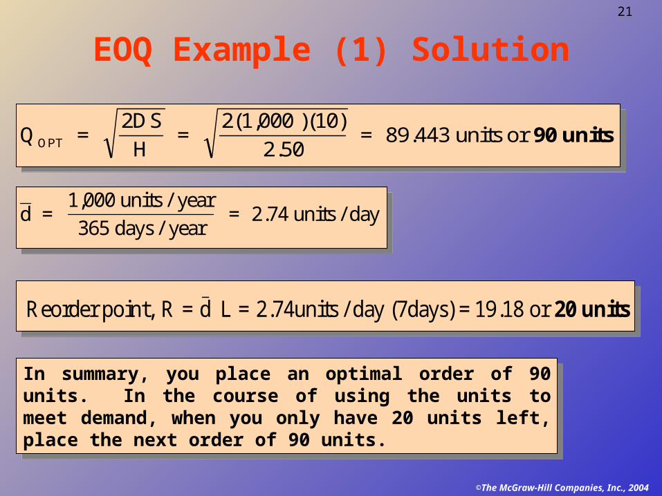
EOQ Example (1) Solution
Q = 2DS
H =
2(1,000 )(10)
2.50 = 89.443 units or OPT 90 unitsQ =
2DS
H =
2(1,000 )(10)
2.50 = 89.443 units or OPT 90 units
d = 1,000 units / year
365 days / year = 2.74 units / dayd =
1,000 units / year
365 days / year = 2.74 units / day
Reorder point, R = d L = 2.74units / day (7days) = 19.18 or _
20 units Reorder point, R = d L = 2.74units / day (7days) = 19.18 or _
20 units
In summary, you place an optimal order of 90 units. In the course of using the units to meet demand, when you only have 20 units left, place the next order of 90 units.
In summary, you place an optimal order of 90 units. In the course of using the units to meet demand, when you only have 20 units left, place the next order of 90 units.

©The McGraw-Hill Companies, Inc., 2004
22
EOQ Example (2) Problem Data
Annual Demand = 10,000 units
Days per year considered in average daily demand = 365
Cost to place an order = $10
Holding cost per unit per year = 10% of cost per unit
Lead time = 10 days
Cost per unit = $15
Determine the economic order quantity and the reorder point given the following…
Determine the economic order quantity and the reorder point given the following…

©The McGraw-Hill Companies, Inc., 2004
23
EOQ Example (2) Solution
Q =2DS
H=
2(10,000 )(10)
1.50= 365.148 units, or OPT 366 unitsQ =
2DS
H=
2(10,000 )(10)
1.50= 365.148 units, or OPT 366 units
d =10,000 units / year
365 days / year= 27.397 units / dayd =
10,000 units / year
365 days / year= 27.397 units / day
R = d L = 27.397 units / day (10 days) = 273.97 or _
274 unitsR = d L = 27.397 units / day (10 days) = 273.97 or _
274 units
Place an order for 366 units. When in the course of using the inventory you are left with only 274 units, place the next order of 366 units.
Place an order for 366 units. When in the course of using the inventory you are left with only 274 units, place the next order of 366 units.

©The McGraw-Hill Companies, Inc., 2004
24
Fixed-Order Quantity Model Model With Safety Stock
• Safety stock:— An amount added to R due to uncertainty of
demand during the lead time— Could be constant or variable (based on known
service level)
Where,
= number of standard deviations for a given service probability
= Standard deviation of usage during the lead time
SSLdR
LzSS
Lz
©The McGraw-Hill Companies, Inc., 2004
25
Fixed-Time Period Model with Safety Stock Formula
order)on items (includes levelinventory current = I
timelead and review over the demand ofdeviation standard =
yprobabilit service specified afor deviations standard ofnumber the= z
demanddaily averageforecast = d
daysin timelead = L
reviewsbetween days ofnumber the= T
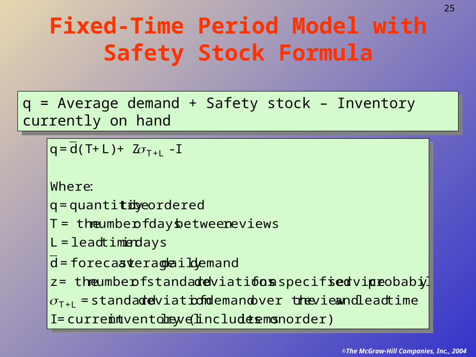
ordered be toquantitiy = q
:Where
I - Z+ L)+(Td = q
L+T
L+T
order)on items (includes levelinventory current = I
timelead and review over the demand ofdeviation standard =
yprobabilit service specified afor deviations standard ofnumber the= z
demanddaily averageforecast = d
daysin timelead = L
reviewsbetween days ofnumber the= T
ordered be toquantitiy = q
:Where
I - Z+ L)+(Td = q
L+T
L+T
q = Average demand + Safety stock – Inventory currently on handq = Average demand + Safety stock – Inventory currently on hand
©The McGraw-Hill Companies, Inc., 2004
26
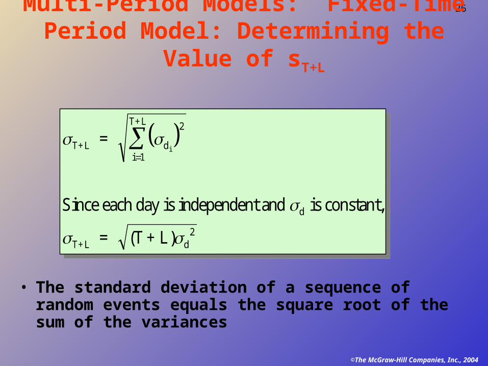
Multi-Period Models: Fixed-Time Period Model: Determining the Value of sT+L
T+ L di 1
T+ L
d
T+ L d2
=
Since each day is independent and is constant,
= (T + L)
i
2
T+ L di 1
T+ L
d
T+ L d2
=
Since each day is independent and is constant,
= (T + L)
i
2
• The standard deviation of a sequence of random events equals the square root of the sum of the variances

©The McGraw-Hill Companies, Inc., 2004
27
Example of the Fixed-Time Period Model
Average daily demand for a product is 20 units. The review period is 30 days, and lead time is 10 days. Management has set a policy of satisfying 96 percent of demand from items in stock. At the beginning of the review period there are 200 units in inventory. The daily demand standard deviation is 4 units.
Given the information below, how many units should be ordered?
Given the information below, how many units should be ordered?

©The McGraw-Hill Companies, Inc., 2004
28
Example of the Fixed-Time Period Model: Solution (Part 1)
T+ L d2 2 = (T + L) = 30 + 10 4 = 25.298 T+ L d
2 2 = (T + L) = 30 + 10 4 = 25.298
The value for “z” is found by using the Excel NORMSINV function, or as we will do here, using Appendix D. By adding 0.5 to all the values in Appendix D and finding the value in the table that comes closest to the service probability, the “z” value can be read by adding the column heading label to the row label.
The value for “z” is found by using the Excel NORMSINV function, or as we will do here, using Appendix D. By adding 0.5 to all the values in Appendix D and finding the value in the table that comes closest to the service probability, the “z” value can be read by adding the column heading label to the row label.
So, by adding 0.5 to the value from Appendix D of 0.4599, we have a probability of 0.9599, which is given by a z = 1.75
So, by adding 0.5 to the value from Appendix D of 0.4599, we have a probability of 0.9599, which is given by a z = 1.75
©The McGraw-Hill Companies, Inc., 2004
29
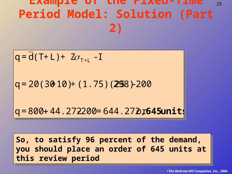
Example of the Fixed-Time Period Model: Solution (Part 2)
or 644.272, = 200 - 44.272 800 = q
200- 298)(1.75)(25. + 10)+20(30 = q
I - Z+ L)+(Td = q L+T
units 645
or 644.272, = 200 - 44.272 800 = q
200- 298)(1.75)(25. + 10)+20(30 = q
I - Z+ L)+(Td = q L+T
units 645
So, to satisfy 96 percent of the demand, you should place an order of 645 units at this review period
So, to satisfy 96 percent of the demand, you should place an order of 645 units at this review period

©The McGraw-Hill Companies, Inc., 2004
30
Variants of EOQ: Price-Break or Discount Models
• Seller offers you incentive to buy more
• Larger lot sizes result in cheaper/unit cost
• Two possibilities:
— Holding cost is constant or variable: Compute Q using the appropriate H
If Q corresponds to lowest price break, it is optimal
Else, find TC for Q and those for lower price breaks
The Q corresponding to lowest TC is optimal

©The McGraw-Hill Companies, Inc., 2004
31
Price-Break (Discount) Model Formula
Cost Holding Annual
Cost) Setupor der Demand)(Or 2(Annual =
iC
2DS = QOPT
Based on the same assumptions as the EOQ model, the price-break model has a similar Qopt formula:
i = percentage of unit cost attributed to carrying inventoryC = cost per unit
Since “C” changes for each price-break, the formula above will have to be used with each price-break cost value

©The McGraw-Hill Companies, Inc., 2004
32
Discount Example: Fixed Holding Cost
• Demand for tires is 12,000 units/year. Normal cost for tires is $30/unit. Orders between 100-499 will cost $27.75/unit, 500-999 will cost $25.5/unit, and 1000 units of more will cost $24/unit. Order cost is $150/order and holding cost is $5/unit/year. What policy should the company adopt?
©The McGraw-Hill Companies, Inc., 2004
33
Discount Example: Variable Holding Cost
• Suppose in the discount tire example that holding cost is charged at 18% of the cost of the tires. What policy should the company adopt?
— The Q could be infeasible
— The Q could be semi-feasible
— The Q could be feasible

©The McGraw-Hill Companies, Inc., 2004
34
Discount Example: VHC Continued
Flagstaff Products offers the following discount schedule for its 4’x8’ sheets of plywood.
Order Quantity Unit Cost
9 Sheets or less $ 18.00
10 to 50 Sheets $ 17.50
More than 50 Sheets $ 17.25
Home Sweet Home Company (HSH) orders plywood from Flagstaff Products. HSH has an ordering cost of $45.00. The carrying cost is 20% of cost, and the annual demand is 100 sheets. What do recommend as the ordering policy for HSH?

©The McGraw-Hill Companies, Inc., 2004
35
Price-Break Example Problem Data (Part 1)
A company has a chance to reduce their inventory ordering costs by placing larger quantity orders using the price-break order quantity schedule below. What should their optimal order quantity be if this company purchases this single inventory item with an e-mail ordering cost of $4, a carrying cost rate of 2% of the inventory cost of the item, and an annual demand of 10,000 units?
A company has a chance to reduce their inventory ordering costs by placing larger quantity orders using the price-break order quantity schedule below. What should their optimal order quantity be if this company purchases this single inventory item with an e-mail ordering cost of $4, a carrying cost rate of 2% of the inventory cost of the item, and an annual demand of 10,000 units?
Order Quantity(units) Price/unit($)0 to 2,499 $1.202,500 to 3,999 1.004,000 or more 0.98

©The McGraw-Hill Companies, Inc., 2004
36
Price-Break Example Solution (Part 2)
units 1,826 = 0.02(1.20)
4)2(10,000)( =
iC
2DS = QOPT
Annual Demand (D)= 10,000 unitsCost to place an order (S)= $4
First, plug data into formula for each price-break value of “C”
units 2,000 = 0.02(1.00)
4)2(10,000)( =
iC
2DS = QOPT
units 2,020 = 0.02(0.98)
4)2(10,000)( =
iC
2DS = QOPT
Carrying cost % of total cost (i)= 2%Cost per unit (C) = $1.20, $1.00, $0.98
Interval from 0 to 2499, the Qopt value is feasible
Interval from 2500-3999, the Qopt value is not feasible
Interval from 4000 & more, the Qopt value is not feasible
Next, determine if the computed Qopt values are feasible or not
©The McGraw-Hill Companies, Inc., 2004
37
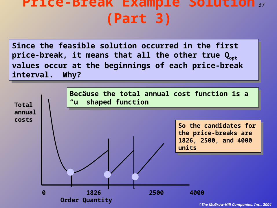
Price-Break Example Solution (Part 3)
Since the feasible solution occurred in the first price-break, it means that all the other true Qopt values occur at the beginnings of each price-break interval. Why?
Since the feasible solution occurred in the first price-break, it means that all the other true Qopt values occur at the beginnings of each price-break interval. Why?
0 1826 2500 4000 Order Quantity
Total annual costs
So the candidates for the price-breaks are 1826, 2500, and 4000 units
So the candidates for the price-breaks are 1826, 2500, and 4000 units
Because the total annual cost function is a “u” shaped function
Because the total annual cost function is a “u” shaped function

©The McGraw-Hill Companies, Inc., 2004
38
Price-Break Example Solution (Part 4)
iC 2
Q + S
Q
D + DC = TC iC
2
Q + S
Q
D + DC = TC
Next, we plug the true Qopt values into the total cost annual cost function to determine the total cost under each price-break
Next, we plug the true Qopt values into the total cost annual cost function to determine the total cost under each price-break
TC(0-2499) =(10000*1.20)+(10000/1826)*4+(1826/2)(0.02*1.20) = $12,043.82TC(2500-3999) = $10,041TC(4000&more) = $9,949.20
TC(0-2499) =(10000*1.20)+(10000/1826)*4+(1826/2)(0.02*1.20) = $12,043.82TC(2500-3999) = $10,041TC(4000&more) = $9,949.20
Finally, we select the least costly Qopt, which is this problem occurs in the 4000 & more interval. In summary, our optimal order quantity is 4000 units
Finally, we select the least costly Qopt, which is this problem occurs in the 4000 & more interval. In summary, our optimal order quantity is 4000 units

©The McGraw-Hill Companies, Inc., 2004
39
Variant of the EOQ: The EPQ Model
• Product produced and consumed simultaneously
• Plant within a plant situation• EOQ definitions apply plus:
— d = constant usage rate— p = production rate
— EPQ =
— TC =
)(
2
dpH
DSp
)(2
)(H
p
dpQDCS
Q
D

©The McGraw-Hill Companies, Inc., 2004
40
EPQ: Example
• A product, X, is assembled with another component, Xi, which is produced in another department at a rate of 100 units/day. The use rate for Xi at assembly department is 40/day. Find optimal production order size, reorder point, and total cost if there are 250 working days/year, S=$50, H=$.5/unit/year, P=$7/Xi, L=7 days, and D=10000.
• Solution:
— EPQ =
— R = dL = 40(7) = 280 units
— TC =
1826)40100(50.0
10050)10000(2
)(
2
dpH
DSp
547,70$)5(.1002
60182671000050
1826
10000
2
)(
Hp
dpQDCS
Q
D

©The McGraw-Hill Companies, Inc., 2004
41
Miscellaneous Systems:Optional Replenishment System
Maximum Inventory Level, M
M Actual Inventory Level, I
q = M - I
I
Q = minimum acceptable order quantity
If q > Q, order q, otherwise do not order any.
©The McGraw-Hill Companies, Inc., 2004
42
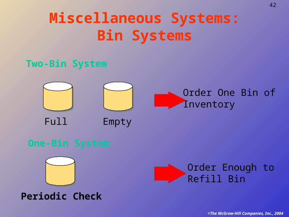
Miscellaneous Systems:Bin Systems
Two-Bin System
Full Empty
Order One Bin ofInventory
One-Bin System
Periodic Check
Order Enough toRefill Bin

©The McGraw-Hill Companies, Inc., 2004
43
ABC Classification System
• Items kept in inventory are not of equal importance in terms of:
— dollars invested
— profit potential
— sales or usage volume
— stock-out penalties
0
30
60
30
60
AB
C
% of $ Value
% of Use
So, identify inventory items based on percentage of total dollar value, where “A” items are roughly top 15 %, “B” items as next 35 %, and the lower 65% are the “C” items

©The McGraw-Hill Companies, Inc., 2004
44
ABC Classification System
• Based on Pareto Study— 20% of people 80% of wealth (80/20 rule)— Used in most areas of business
• The scheme
— Class A items Fewest in number—10-20% Highest in dollar value—70-80% Exercise greatest control here
©The McGraw-Hill Companies, Inc., 2004
45
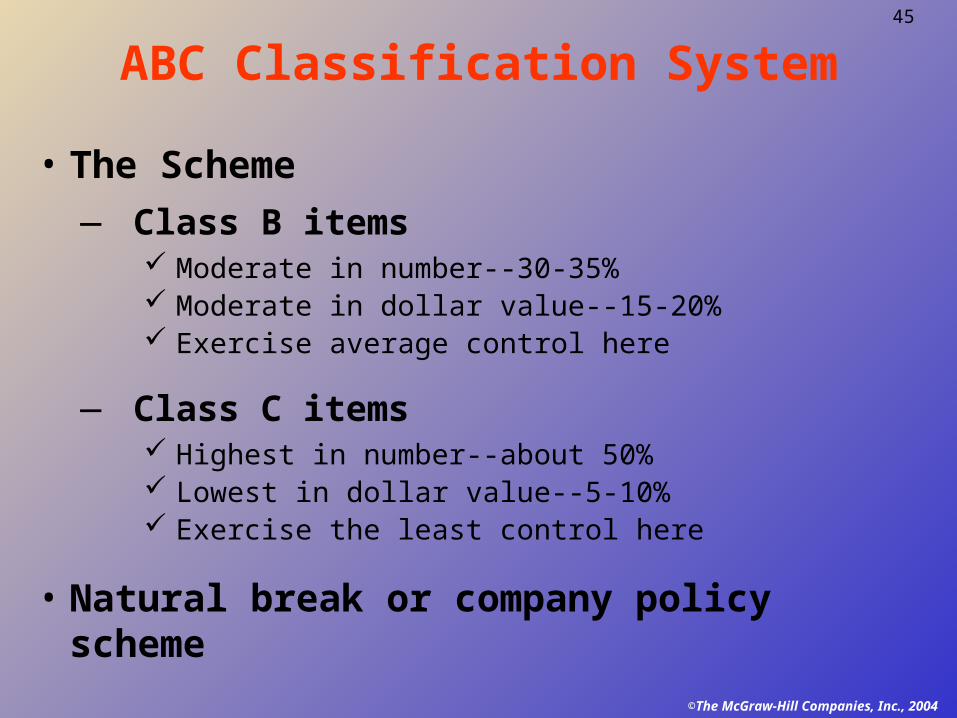
ABC Classification System
• The Scheme
— Class B items Moderate in number--30-35% Moderate in dollar value--15-20% Exercise average control here
— Class C items Highest in number--about 50% Lowest in dollar value--5-10% Exercise the least control here
• Natural break or company policy scheme
©The McGraw-Hill Companies, Inc., 2004
46
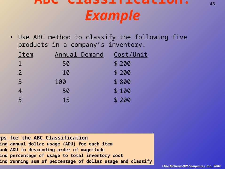
ABC Classification: Example• Use ABC method to classify the following five products in a company’s
inventory.
Item Annual Demand Cost/Unit
1 50 $ 200
2 10 $ 200
3 100 $ 800
4 50 $ 100
5 15 $ 200
Steps for the ABC Classification• Find annual dollar usage (ADU) for each item• Rank ADU in descending order of magnitude• Find percentage of usage to total inventory cost• Find running sum of percentage of dollar usage and classify

©The McGraw-Hill Companies, Inc., 2004
47
Inventory Accuracy and Cycle CountingDefined
• Inventory accuracy refers to how well the inventory records agree with physical count
• Cycle Counting is a physical inventory-taking technique in which inventory is counted on a frequent basis rather than once or twice a year