, Ran Jin , V. Roshan Joseph a -...

StatThe ISI’s Journal for the Rapid (wileyonlinelibrary.com) DOI: 10.1002/sta4.26Dissemination of Statistics Research

Gaussian process modeling for engineeredsurfaces with applications to Si wafer productionMatthew Plumleea,�, Ran Jinb, V. Roshan Josepha and Jianjun Shia

Received 18 June 2013; Accepted 9 July 2013

When producing engineered surfaces, the stochastic portion of the processing greatly affects the overall outputquality. We propose a Gaussian process model that accounts for the impact of control variables on the stochasticelements of the produced surfaces. An optimization algorithm is outlined to find the maximum likelihood estimatesof the model parameters. A case study involving the thickness surfaces of semiconductor wafers is examined thatdemonstrates the need for the proposed approach. Copyright © 2013 John Wiley & Sons, Ltd.

Keywords: designed experiment; functional response; quality control; statistical process control

1 IntroductionThe material surface is of critical importance because of its impact on the downstream properties of products such asfriction and optical behavior. We study the case where we receive measurements from surfaces created via controlledproduction or “engineered”. Data from engineered surfaces have become pervasive in recent years because of devel-opments in measurement technology, information storage capacity, and processing power. A large amount of statisticalresearch has studied monitoring processes that produce surfaces (typically termed profiles). Monitoring is usually per-formed by explicitly modeling a given surface (e.g., Qiu et al. (2010)). Our paper presents a different direction. Ourgoal is not to explicitly model a given surface but instead to model the stochastic distribution of produced surfaces.We study this distribution as the process inputs are altered. This problem is similar to a regression problem with func-tional responses (Faraway, 1997). The core difference between this work and the works found in the current literatureis the focus on the stochastic portion of the responses.

We study the scenario where a user has the capability to alter certain variables, which we will denote control variablesor u. Surface measurements (Y) are collected corresponding to a set of explanatory variables (x) that represent thespatial location of the measurement. This paper addresses the challenge of incorporating control variables into theanalysis of systems with stochastic surface responses. As an example, Section 4 studies wire-sawn semiconductorwafers exhibiting undesirable waviness. Lapping, a process in which a liquid slurry containing abrasive particles ispressed onto a rotating surface, is used to reduce waviness. Here, control variables include the downward pressure andthe rotation speed of the lapping pad. Table I outlines the response of a lapping process to a 24�1 fractional factorialdesign of experiments with one center run; see Wu & Hamada (2009) for more information on designed experiments.

aH. Milton Stewart School of Industrial and Systems Engineering, Georgia Institute of Technology, Atlanta, GA 30318, USAbGrado Department of Industrial and Systems Engineering, Virginia Institute of Technology, Blacksburg, VA 24061, USA∗Email: [email protected]

Stat 2013; 2: 159–170 Copyright © 2013 John Wiley & Sons Ltd

M. Plumlee et al. Stat(wileyonlinelibrary.com) DOI: 10.1002/sta4.26 The ISI’s Journal for the Rapid

Dissemination of Statistics Research

Table I. Designed experiment for a lapping process.

Control variables uRun plow RPM tlow thigh Profile data1 + � � � Y1,1 Y1,2 . . . Y1,d1

2 + + � + Y2,1 Y2,2 . . . Y2,d2

3 � � � + Y3,1 Y3,2 . . . Y3,d3

4 � � + � Y4,1 Y4,2 . . . Y4,d4

5 � + � � Y5,1 Y5,2 . . . Y5,d5

6 + � + + Y6,1 Y6,2 . . . Y6,d6

7 + + + � Y7,1 Y7,2 . . . Y7,d7

8 � + + + Y8,1 Y8,2 . . . Y8,d8

9 0 0 0 0 Y9,1 Y9,2 . . . Y9,d9

The data, YTij D[ Yij.x1/, : : : , Yij.xn/], consist of over 150 thickness measurements on a regular grid .x1, : : : , xn/ on wafer

j produced at experimental index i.

Research has been reported to model the relationship between the control variables and the engineered surfaces byusing physical or mechanical knowledge. However, these models are often deterministic and lack the ability to dealwith the inherent stochasticity. The stochastic behavior of the system cannot be ignored for analysis as a multitudeof studies have found that topology related to stochastic variation affects the output quality (e.g., surface friction, seeBhushan (2003)). Furthermore, there has been evidence that stochastic elements are affected by the processing used;see Pei (2002) for an example involving a grinding process applied to silicon wafers.

Toward the aim of modeling the stochastic behavior of the system, we introduce a uniquely parameterized versionof a Gaussian process model. Gaussian process models have found extensive use in areas such as geostatistics,environmental science, and computer experiments; see the works of Matheron (1963), Sansó & Guenni (2000), andSantner et al. (2003) for examples. The power of this model is the ability to account for varying levels differentiabilityand continuity of a surface. For a more complete history of literature relating to spatial statistics, see Gelfand et al.(2010).

The core contribution of this paper is the proposed model for the interaction of control variables and stochasticbehavior, outlined in Section 2. In Section 3, an iterative optimization technique for finding maximum likelihoodestimates (MLEs) for the model is discussed. Section 4 outlines a case study for this model that verifies the need tomodel stochastic behavior as a function of the control variables. Additionally, Section 4 describes a surface modeldefined on polar coordinates for silicon wafers produced via a rotational mechanism. Section 5 includes conclusionsand outlines possible future work.

2 Proposed modeling frameworkThe model discussed in this paper will emulate semi-parametric models such as those seen in Zeger & Diggle (1994),replacing the spline model with a Gaussian process. This is justified by the connections between processes generatedby spline basis functions and Gaussian process models; see, for example, Wahba (1978). Each experimental indexi corresponds to a set of control variables denoted ui. The model of the kth point on the jth surface generated atexperimental index i is described as

Yijk.ui, xk/ D �.xk;ˇ.ui//C Zj�xk; �.ui/, �2.ui/

�C �ijk, (1)

Copyright © 2013 John Wiley & Sons Ltd 160 Stat 2013; 2: 159–170

Stat Engineered surface modeling

The ISI’s Journal for the Rapid (wileyonlinelibrary.com) DOI: 10.1002/sta4.26Dissemination of Statistics Research

where �, Z, and � represent the underlying mean, a stochastic error due to processing, and measurement noise,respectively. Values of measurement noise are modeled as independent and normal, �ijk � N [ 0, �2� ]. The mean ismodeled as an additive linear model with a set of basis functions fx.x/ that map x to Rp, that is, �.x;ˇ.u// DfTx .x/ˇ.u/. The proper choice of a set of basis functions for the mean depends on the particular application. In

Section 4, we use a general set of spline basis functions for fx combined with a basis function that incorporatesengineering knowledge. The modeling of Zj will take the form of an independent realization of the Gaussian process,

Zj�x; �.u/, �2.u/

�� GP

�0, �2.u/R.�, �; �.u//

�,

where �2.u/ and �.u/ are the variance and correlation parameters of the process.

The Gaussian process model assumes that any collection of points on a surface follows a multivariate normal dis-tribution that depends on the variance, Var.Zj.x1// D �2.u/, and the correlation function, Corr¹Zj.x1/, Zj.x2/º DR.x1, x2; �.u//. The correlation function, R, is a positive definite function that dictates the correlation between anytwo points on a surface. For more information on the properties and development of correlation functions, see Gelfandet al. (2010). Several correlation functions exist, including the powered exponential class, the Matérn class (Matérn,1986), and the Cauchy class (Gneiting & Schlather, 2004). The Gaussian process model is useful in this circum-stance because it has the power to account for the underlying continuity of the surface. Using the Gaussian processassumption also creates the ability to use available maximum likelihood-based methods for estimating the parametersof the model.

The core idea of this paper is the following: the parameters of the surfaces, especially ones that dictate stochasticbehavior, ought to be modeled as a function of the control variables. In terms of the proposed model, the meanparameter (ˇ.u/), the correlation parameter (�.u/), and the variance of the surface (�2.u/) are assumed to changewith the control variables. This implies that the control variables affect not only the mean but also the stochasticportion of the surface model.

Because of the high cost associated with performing designed experiments in wafer manufacturing (both in terms ofmaterial and measurement costs), it is common for few design points to be present in experiments such as Table I.As a result, it is reasonable to use a linear model with higher order terms to represent how u interacts with thesurface parameters. The functions ˇ.u/, �2.u/, and �.u/ are therefore modeled as linear combinations of a set of basisfunctions fu.u/ that map a value of u to Rq. Let A 2 Rq�p, ˛� 2 Rq, and ˛� 2 Rq; the functions are ˇ.u/ D Afu.u/,log �2.u/ D ˛T

� fu.u/, and g.�.u// D ˛T�fu.u/, where g is a link function (e.g., a log-link function for a strictly positive

quantity). These functions are not known explicitly, and they depend on parameters A, ˛� , and ˛� , respectively. Wepropose estimating these parameters via the algorithm in Section 3. The same basis function, fu.u/, is assumed foreach parameter ˇ.u/, �2.u/, and �.u/. This is not a requirement, but it often simplifies notation and allows for theprocedure outlined in this paper to be generally applicable.

3 Parameter estimationThe model described in the previous section has limited usability without valid parameter estimates. In this paper,parameter estimates will be determined by the maximum likelihood criterion. Given the complex structure of themodel, closed-form estimates for all parameters could not be reached. Additionally, the amount of data present inexperiments such as those seen in Table I makes Markov chain Monte Carlo techniques intractable. This section willdetail an iterative method to find MLEs.

There is a simplified parameterization of the mean using properties of Kronecker products, ˝. The expression for themean vector is simplified to

Stat 2013; 2: 159–170 161 Copyright © 2013 John Wiley & Sons Ltd



�.u/ D Fxˇ.u/,

D FxAfTu.u/,

D�Fx ˝ fT

u.u/�

vec.A/,

D�Fx ˝ fT

u.u/��,

where �T.u/ D[�.x1;ˇ.u//, : : : ,�.xn;ˇ.u//], Fx is defined as FTx D[ fx.x1/, : : : , fx.xn/], and � is the new parameter

for the mean of the model.

By the model in (1), Yij � Nn[�.ui/, �2i .R.�i/ C �2� I/], where �i D �.ui;˛� / and �2i D �2.ui;˛� /. The matrix R.�i/

is the surface correlation matrix composed of elements ¹R.�i/ºlk D R.xl, xk; �i/. The total negative log-likelihood istherefore proportional to (up to a constant)

l DmX

iD1

diXjD1

´nlog

��2i�C log

�jR�i j

�C

rTijR��1i rij

�2i

μ, (2)

where m is the number of runs in the experiment, rTij D .Yij � .Fx ˝ fT

u.ui//�/T, and R�i D R.�i/ C

�2��2i

I. Minimizing

(2) is equivalent to maximizing the likelihood. The maximum likelihood estimate of the mean parameter, �, has aclosed-form solution, given the parameters ˛� and ˛� ,

O� D

24 mX

iD1

diXjD1

1

�2i

�Fx ˝ fT

u.ui/�T

R��1i

�Fx ˝ fT

u.ui/�35�124 mX

iD1

diXjD1

1

�2i

�Fx ˝ fT

u.ui/�T

R��1i Yij

35 . (3)

The MLE estimate of the parameter ˛� also exhibits simplifications using the following proposition:

Proposition 3.1Assume Yi, i D 1, : : : , m, follows a multivariate normal distribution with mean �.ui/ and covariance �2.ui/R.ui/.Assume that �.ui/ and R.ui/ are given and �2.ui/ D ˛T

� fu.ui/. The generalized linear model estimate (Nelder &Wedderburn, 1972) of ˛� , with gamma distribution, input vectors fu.u1/, : : : , fu.um/ and a log-link function, to theresponse �21 , : : : , �2m, where �2i D

1n .Yi ��.ui//

TR�1.ui/.Yi ��.ui//, is equal to the maximum likelihood estimate of˛� .

The preceding result is easily derived from the definition of generalized linear models. This demonstrates that we canuse popular software methods to find numerical estimates for ˛� .

Using the preceding results, we construct an optimization algorithm that finds the MLEs of a group of parametersgiven all other parameters. This idea is similar in spirit to the classic EM algorithm (Dempster et al., 1977) viewedas an iterative maximization problem (Neal & Hinton, 1998). The parameters are grouped as ¹˛� , ��º, ˛� , and �. Wedenote each iterate with the superscript ¹kº and suppress the two superscripts in the variance terms for clarity. Thealgorithm is as follows:

1. Initialize � ¹0ºi , � ¹0ºi , and � ¹0º�,i for each experimental index i. Set k D 0.

2. Use � ¹0ºi and � ¹0ºi to initialize ˛¹0º�

, ˛¹0º� via least squares regression and initialize � ¹0º� D 1m

Pi �¹0º�,i .

3. Set � ¹kºi D �2�ui;˛

¹kº�

�, � ¹kºi D �

�ui;˛

¹kº�

�, and R�i D R

��¹kºi

�C �

¹kº�

�¹kºi

I for all i D 1, : : : , m.

4. Estimate �¹kC1º via (3) using R�i and � ¹kºi .




5. Estimate the variance term for each surface via

�2ij D

�Yij �

�Fx ˝ fT

u .ui/��¹kC1º

�TR��1i

�Yij �

�Fx ˝ fT

u .ui/��¹kC1º

�n

.

Fit a GLM with a log link with response �2ij , an input vector fu .ui/, and a gamma distribution to yield ˛¹kC1º� .

Set � ¹kC1ºi D �2�ui;˛

¹kC1º�

�and R�i D R.� ¹kºi /C �

¹kC1º�

�¹kºi

I. Repeat to convergence of ˛¹kC1º� .

6. Use a generic optimization algorithm to maximize the likelihood given in (2) using � D �¹kC1º and �i D �¹kC1ºi ,

i D 1, : : : , m, to choose ˛¹kC1º�

and � ¹kC1º� . Set � ¹kC1ºi D ��ui;˛

¹kC1º�

�, and R�i D R

��¹kC1ºi

�C �

¹kC1º�

�¹kC1ºi

I.

7. Repeat 4 to 6 until convergence.

This iterative formulation reduces the computational burden for the likelihood by exploiting known partial maximizationin steps 4 and 5. One might question the convergence of the preceding algorithm. The estimates will converge to thetrue MLEs if the negative log-likelihood is convex with respect to all parameters because we are continually improving.However, there is no guarantee of convexity. But, with adequate initialization, good estimates can be obtained. Initialestimates of � ¹0ºi , � ¹0ºi , and � ¹0º

�,i can be found via several statistical packages by fitting a Gaussian process model toeach surface Yi1, : : : , Yidi and averaging the result.

4 Case study: Si wafer thickness variation aftermechanical lapping

The geometric uniformity of the silicon wafers determines the incoming variation for the downstream processing tocreate products such as integrated circuits and solar cells. Thus, this uniformity is a major control objective in wafermanufacturing. This section presents analysis of a designed experiment to better understand the effect of a set ofcontrol variables on a wafer flattening procedure.

4.1. Background and experimental descriptionWire sawing is the most common approach to slice large-diameter silicon crystal ingots into wafers. Wire sawing canlead to undesirable waviness in final product (Yasunaga et al., 1997), which may be due to the vibrations presentin the wire (Zhao et al., 2011). Flattening procedures, which include lapping, grinding, and chemical–mechanicalpolishing (CMP), are used to reduce the waviness in the final product. For more details on the processes involved inthe production of wafers, see Evans et al. (2003) and Pei et al. (2003).

Significant work has been carried out in the study of these flattening procedures, and majority of work has beenfocused in two areas:

Deterministic differential equation models An example of the differential equation methods can be seen inFu et al. (2001), which develops a model that uses plasticity properties of the surface material to study CMP. Sim-ilar developments have been made in both lapping (Chang et al., 2000) and grinding (Pietsch & Kerstan, 2005).

Feature extraction This method consists of first extracting a feature from each surface. After feature extraction,traditional analysis of experiments is performed where the extracted feature is modeled as the response (e.g.,Zhang et al. (2007)). An example of an extracted feature is total thickness variation (TTV), which is computed bysubtracting the smallest thickness measurement from the largest thickness measurement on a single wafer.




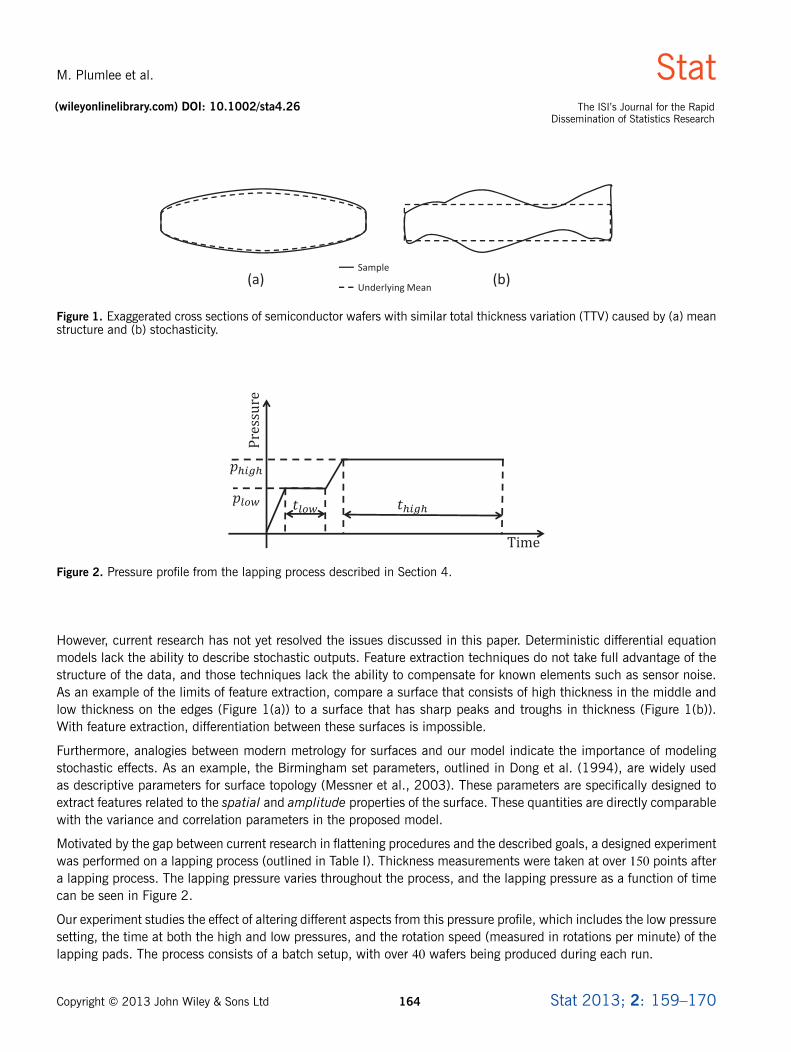
Figure 1. Exaggerated cross sections of semiconductor wafers with similar total thickness variation (TTV) caused by (a) meanstructure and (b) stochasticity.

Figure 2. Pressure profile from the lapping process described in Section 4.

However, current research has not yet resolved the issues discussed in this paper. Deterministic differential equationmodels lack the ability to describe stochastic outputs. Feature extraction techniques do not take full advantage of thestructure of the data, and those techniques lack the ability to compensate for known elements such as sensor noise.As an example of the limits of feature extraction, compare a surface that consists of high thickness in the middle andlow thickness on the edges (Figure 1(a)) to a surface that has sharp peaks and troughs in thickness (Figure 1(b)).With feature extraction, differentiation between these surfaces is impossible.

Furthermore, analogies between modern metrology for surfaces and our model indicate the importance of modelingstochastic effects. As an example, the Birmingham set parameters, outlined in Dong et al. (1994), are widely usedas descriptive parameters for surface topology (Messner et al., 2003). These parameters are specifically designed toextract features related to the spatial and amplitude properties of the surface. These quantities are directly comparablewith the variance and correlation parameters in the proposed model.

Motivated by the gap between current research in flattening procedures and the described goals, a designed experimentwas performed on a lapping process (outlined in Table I). Thickness measurements were taken at over 150 points aftera lapping process. The lapping pressure varies throughout the process, and the lapping pressure as a function of timecan be seen in Figure 2.

Our experiment studies the effect of altering different aspects from this pressure profile, which includes the low pressuresetting, the time at both the high and low pressures, and the rotation speed (measured in rotations per minute) of thelapping pads. The process consists of a batch setup, with over 40 wafers being produced during each run.




4.2. Exploratory data analysisThe measurement locations are shown in Figure 3 and are indexed in a counterclockwise spiral direction from insideto out starting at angle =2. The lapping process grinds fine particles on a rotating surface. Because of this flatteningmechanism, the use of Cartesian coordinates to analyze the mean and correlation structures would produce crypticresults. Therefore, we use polar coordinates to examine the mean and correlation functions.

To study the properties of the mean and correlation functions, we first directly calculate the sample mean vector andthe sample correlation matrices from each of the experimental indices i. Using this estimate directly for analysis isnot considered a stable procedure because the number of points on a surface (150) exceeds the number of surfaceobservations (� 40) in this case study. This is a common problem in applications relating to surface engineering andother functional responses. However, these computations are still useful for exploratory analysis.

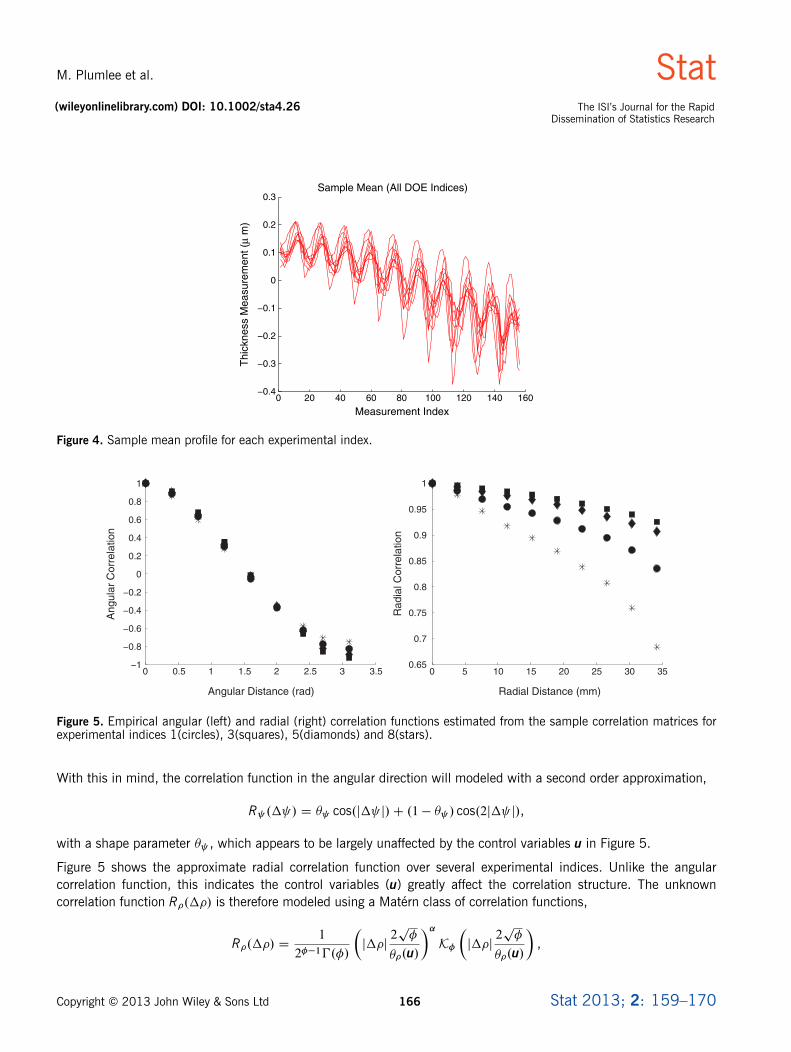
Figure 4 shows the sample mean profile for all nine experimental indices. From this figure, a clear negative sloperelationship between the thickness measurement and the radial distance is present, along with local deviations fromthe general trend. The negative relationship between radial distance and thickness has been observed in mechanicalpolishing of wafers (Pietsch & Kerstan, 2005) and a similar trend is confirmed here. The global mean trend is modeledwith the function �.x/, where �.x/ represents the radial distance from the center of the wafer. To model the localmean function, a set of cubic-spline basis functions, defined on polar coordinates, is used with knot points shown inFigure 3. These two functions comprise a basis set of functions for each surface, that is, fx.x/ discussed in Section 2.

The sample correlation is useful for investigating properties of the correlation functions. Here, we consider empir-ical approximations of the correlation functions computed by averaging the estimated correlation coefficients ofany two points that differ by the same distance, yielding empirical measurements of a stationary correlation func-tion, termed QR.� ,��/. We examine at the correlation function by studying the empirical angular correlation,QR .� / D QR.� , 0/, and the empirical radial correlation, QR�.��/ D QR.0,��/.

Figure 5 shows the empirical angular correlation function over several experimental indices. As shown in Gaspari& Cohn (1999), for a surface in two dimensions, a valid stationary correlation function of � , where � is thedifference in the angle between two points, must take the form of R.� / D

P1kD0 ak cos.k� / with

P1kD0 ak D 1.

−60 −40 −20 0 20 40 60−60

−40

−20

0

20

40

60Measurement Points and Spline Knot Locations

Horizontal Location (mm)

Ver

tical

Loc

atio

n (m

m)

Figure 3. Measurement locations for each wafer marked with ı. Spline knot locations marked with ˝.




0 20 40 60 80 100 120 140 160−0.4

−0.3

−0.2

−0.1

0

0.1

0.2

0.3Sample Mean (All DOE Indices)

Measurement Index

Thi

ckne

ss M

easu

rem

ent (

µ m

)

Figure 4. Sample mean profile for each experimental index.

0 0.5 1 1.5 2 2.5 3 3.5−1

−0.8

−0.6

−0.4

−0.2

0

0.2

0.4

0.6

0.8

1

Ang

ular

Cor

rela

tion

Angular Distance (rad)

0 5 10 15 20 25 30 350.65

0.7

0.75

0.8

0.85

0.9

0.95

1

Rad

ial C

orre

latio

n

Radial Distance (mm)

Figure 5. Empirical angular (left) and radial (right) correlation functions estimated from the sample correlation matrices forexperimental indices 1(circles), 3(squares), 5(diamonds) and 8(stars).

With this in mind, the correlation function in the angular direction will modeled with a second order approximation,

R .� / D � cos.j� j/C .1 � � / cos.2j� j/,

with a shape parameter � , which appears to be largely unaffected by the control variables u in Figure 5.

Figure 5 shows the approximate radial correlation function over several experimental indices. Unlike the angularcorrelation function, this indicates the control variables (u) greatly affect the correlation structure. The unknowncorrelation function R�.��/ is therefore modeled using a Matérn class of correlation functions,

R�.��/ D1

2��1./

�j��j

2p

��.u/

˛K�

�j��j

2p

��.u/

,




where K� is the modified Bessel function of order . Here, �� is strongly affected by u; therefore, this will be modeledby the linear function described Section 2. In total, the correlation function will be modeled by the outer product ofR and R�,

R.� ,��/ D R .� /R�.��/.

4.3. Results from parameter estimation and verification of modelsignificance

The focal point of this paper is the introduction of control variables, u, to the stochastic parameters of the Gaussianprocess error term. This section will justify the need for this modeling through a comparison with a model withconstant stochastic parameters. For simplicity, we compare two models of increasing complexity:

[M0] Model (1) with assumptions �2.u/ D �2 and ��.u/ D ��, that is, both are constant functions.[M1] Model (1) where the functions �2.u/ and ��.u/ will be assumed to be a linear functions of u, as outlined inprevious sections.

Both models will have parameters chosen via the maximum likelihood criterion.

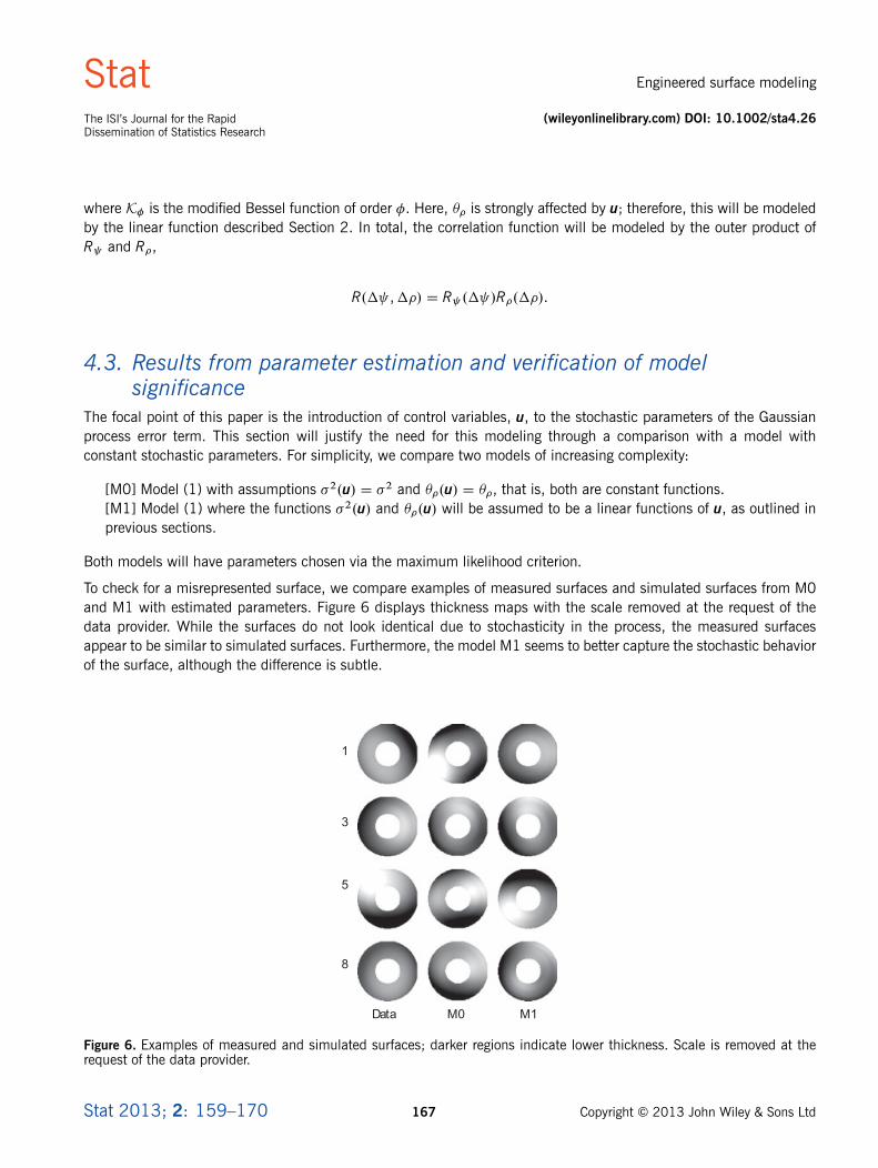
To check for a misrepresented surface, we compare examples of measured surfaces and simulated surfaces from M0and M1 with estimated parameters. Figure 6 displays thickness maps with the scale removed at the request of thedata provider. While the surfaces do not look identical due to stochasticity in the process, the measured surfacesappear to be similar to simulated surfaces. Furthermore, the model M1 seems to better capture the stochastic behaviorof the surface, although the difference is subtle.

Figure 6. Examples of measured and simulated surfaces; darker regions indicate lower thickness. Scale is removed at therequest of the data provider.




Table II. Model selection criteria.

Model M0 M1

ln L 0 4482.6BIC 413.8388 �1742.2

1 2 3 4 5 6 7 8 9

(a)1 2 3 4 5 6 7 8 9

(b)1 2 3 4 5 6 7 8 9

(c)

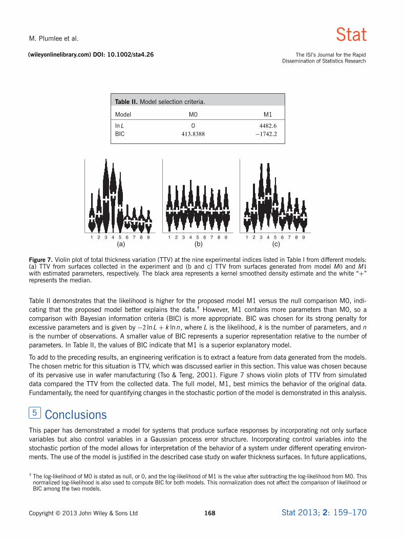
Figure 7. Violin plot of total thickness variation (TTV) at the nine experimental indices listed in Table I from different models:(a) TTV from surfaces collected in the experiment and (b and c) TTV from surfaces generated from model M0 and M1with estimated parameters, respectively. The black area represents a kernel smoothed density estimate and the white “C”represents the median.

Table II demonstrates that the likelihood is higher for the proposed model M1 versus the null comparison M0, indi-cating that the proposed model better explains the data.� However, M1 contains more parameters than M0, so acomparison with Bayesian information criteria (BIC) is more appropriate. BIC was chosen for its strong penalty forexcessive parameters and is given by �2 ln LC k ln n, where L is the likelihood, k is the number of parameters, and nis the number of observations. A smaller value of BIC represents a superior representation relative to the number ofparameters. In Table II, the values of BIC indicate that M1 is a superior explanatory model.

To add to the preceding results, an engineering verification is to extract a feature from data generated from the models.The chosen metric for this situation is TTV, which was discussed earlier in this section. This value was chosen becauseof its pervasive use in wafer manufacturing (Tso & Teng, 2001). Figure 7 shows violin plots of TTV from simulateddata compared the TTV from the collected data. The full model, M1, best mimics the behavior of the original data.Fundamentally, the need for quantifying changes in the stochastic portion of the model is demonstrated in this analysis.

5 ConclusionsThis paper has demonstrated a model for systems that produce surface responses by incorporating not only surfacevariables but also control variables in a Gaussian process error structure. Incorporating control variables into thestochastic portion of the model allows for interpretation of the behavior of a system under different operating environ-ments. The use of the model is justified in the described case study on wafer thickness surfaces. In future applications,

� The log-likelihood of M0 is stated as null, or 0, and the log-likelihood of M1 is the value after subtracting the log-likelihood from M0. Thisnormalized log-likelihood is also used to compute BIC for both models. This normalization does not affect the comparison of likelihood orBIC among the two models.




using different aspects of this model, but not the full model, might be beneficial. For example, Chang et al. (2012)studied nanoparticle dispersion, where the correlation structure is considered a function of the physical properties ofthe atom and does not change with control variables.

AcknowledgementThis research was supported by the US National Science Foundation grant CMMI-1030125.

ReferencesBhushan, B (2003), ‘Adhesion and stiction: mechanisms, measurement techniques, and methods for reduction’,

Journal of Vacuum Science & Technology B: Microelectronics and Nanometer Structures, 21, 2262–2296.

Chang, CJ, Xu, L, Huang, Q & Shi, J (2012), ‘Quantitative characterization and modeling strategy of nanoparticledispersion in polymer composites’, IIE Transactions, 44, 523–533.

Chang, Y, Hashimura, M & Dornfeld, D (2000), ‘An investigation of material removal mechanisms in lapping withgrain size transition’, Journal of Manufacturing Science and Engineering, 122, 413–419.

Dempster, A, Laird, N & Rubin, D (1977), ‘Maximum likelihood from incomplete data via the EM algorithm’, Journalof the Royal Statistical Society. Series B, 39, 1–38.

Dong, WP, Sullivan, PJ & Stout, KJ (1994), ‘Comprehensive study of parameters for characterising three-dimensionalsurface topography IV: parameters for characterising spatial and hybrid properties’, Wear, 178, 45–60.

Evans, CJ, Paul, E, Dornfeld, D, Lucca, DA, Byrne, G, Tricard, M, Klocke, F, Dambon, O & Mullany, BA (2003),‘Material removal mechanisms in lapping and polishing’, CIRP Annals-Manufacturing Technology, 52, 611–633.

Faraway, JJ (1997), ‘Regression analysis for a functional response’, Technometrics, 39, 254–261.

Fu, G, Chandra, A, Guha, S & Subhash, G (2001), ‘A plasticity-based model of material removal in chemical–mechanical polishing (CMP)’, IEEE Transactions on Semiconductor Manufacturing, 14, 406–417.

Gaspari, G & Cohn, S (1999), ‘Construction of correlation functions in two and three dimensions’, Quarterly Journalof the Royal Meteorological Society, 125, 723–757.

Gelfand, A, Diggle, P, Fuentes, M & Guttorp, P (2010), Handbook of Spatial Statistics, CRC Press.

Gneiting, T & Schlather, M (2004), ‘Stochastic models that separate fractal dimension and the Hurst effect’, SIAMReview, 46, 269–282.

Matérn, B (1986), Spatial Variation, 2nd edn., Springer-Verlag, Berlin.

Matheron, G (1963), ‘Principles of geostatistics’, Economic Geology, 58, 1246–1266.

Messner, C, Silberschmidt, V & Werner, E (2003), ‘Thermally induced surface roughness in austenitic–ferritic duplexstainless steels’, Acta Materialia, 51, 1525–1537.

Neal, RM & Hinton, GE (1998), ‘A view of the EM algorithm that justifies incremental, sparse, and other variants’, inLearning in Graphical Models, Springer, pp. 355–368.




Nelder, JA & Wedderburn, RW (1972), ‘Generalized linear models’, Journal of the Royal Statistical Society.Series A, 135, 370–384.

Pei, Z (2002), ‘A study on surface grinding of 300 mm silicon wafers’, International Journal of Machine Tools andManufacture, 42, 385–393.

Pei, ZJ, Xin, XJ & Liu, W (2003), ‘Finite element analysis for grinding of wire-sawn silicon wafers: a designedexperiment’, International Journal of Machine Tools and Manufacture, 43, 7–16.

Pietsch, GJ & Kerstan, M (2005), ‘Understanding simultaneous double-disk grinding: operation principle and materialremoval kinematics in silicon wafer planarization’, Precision Engineering, 29, 189–196.

Qiu, P, Zou, C & Wang, Z (2010), ‘Nonparametric profile monitoring by mixed effects modeling’, Technometrics, 52,265–277.

Sansó, B & Guenni, L (2000), ‘A nonstationary multisite model for rainfall’, Journal of the American StatisticalAssociation, 95, 1089–1100.

Santner, TJ, Williams, BJ & Notz, W (2003), The Design and Analysis of Computer Experiments, Springer Verlag.

Tso, PL & Teng, CC (2001), ‘A study of the total thickness variation in the grinding of ultra-precision substrates’,Journal of Materials Processing Technology, 116, 182–188.

Wahba, G (1978), ‘Improper priors, spline smoothing and the problem of guarding against model errors in regression’,Journal of the Royal Statistical Society. Series B (Methodological), 40, 364–372.

Wu, CFJ & Hamada, M (2009), Experiments: Planning, Analysis, and Optimization, 2nd edn., Wiley New York.

Yasunaga, N, Takashina, M & Itoh, T (1997), ‘Development of sequential grinding-polishing process applicable tolarge-size Si wafer finishing’, in Proceedings of the International Symposium on Advances in Abrasive Technology,Sydney, Australia, pp. 96–100.

Zeger, S & Diggle, P (1994), ‘Semiparametric models for longitudinal data with application to CD4 cell numbers inHIV seroconverters’, Biometrics, 50, 689–699.

Zhang, JZ, Chen, JC & Kirby, ED (2007), ‘Surface roughness optimization in an end-milling operation using theTaguchi design method’, Journal of Materials Processing Technology, 184, 233–239.

Zhao, H, Jin, R, Wu, S & Shi, J (2011), ‘PDE-constrained Gaussian process model on material removal rate of wiresaw slicing process’, Journal of Manufacturing Science and Engineering, 133.


, Ran Jin , V. Roshan Joseph a -...

Documents

Transcript of , Ran Jin , V. Roshan Joseph a -...