© Rahmatullah Ibrahim Nuruddeen - core.ac.uk · 1.1Literature Review 3 ... 2.4.3 Extended form of...
90
Transcript of © Rahmatullah Ibrahim Nuruddeen - core.ac.uk · 1.1Literature Review 3 ... 2.4.3 Extended form of...


i
© Rahmatullah Ibrahim Nuruddeen
October, 2015

ii
To My Family

iii
ACKNOWLEDGEMENTS
All praises is for Allah (S.W.T.), the most high, most gracious and most merciful. May
His peace, blessings and mercy be upon His noble messenger and prophet Muhammad
(S.A.W), his family, his companions, and those who follow their footsteps till the last
day.
Firstly, I would like to start by expressing my profound gratitude and indebtedness to my
supervisor Prof. Fiazud Din Zaman for introducing me to this area, and for his inspiring
guidance, endless support and valuable suggestion throughout this work. I also like to
acknowledge the guidance received from my committee members Prof. Rajai Samih
Mousa Alassar and Prof. Ashfaque Hussain Bokhari through their various suggestions
and inputs during this research. Furthermore, I would like to thank the chairman, Dr.
Husain Salem Al-Attas and the entire faculty and staff of mathematics and statistics
department, for their support and encouragement. I also thank the Kingdom of Saudi
Arabia and King Fahd University of Petroleum & Minerals for providing me with the
scholarship package.
My heartfelt thanks, gratefulness and appreciations go to my parents for their unending
love, support, encouragement and prayers. I pray to Allah to strengthen their faith and
grant them Jannah. Lastly, I would like to appreciate each and everybody, ranging from
family, relatives, friends, and all who have contributed in one way or the other towards
the successful completion of this program, may Allah reward them all.

iv
TABLE OF CONTENTS ACKNOWLEDGEMENTS iii TABLE OF CONTENTS iv LIST OF FIGURES vi ABSTRACT (ENGLISH) vii ABSTRACT (ARABIC) viii
CHAPTER ONE: INTRODUCTION AND LITERATURE REVIEW
1.0 Introduction 1 1.1Literature Review 3 1.2 Basic Definitions of Some Terms 6
1.2.1 Bessel Differential Equation 6 1.2.2 Solution of the Bessel Differential Equation 6 1.2.3 Modified Bessel Differential Equation 6 1.2.4 Solution of the Modified Bessel Differential Equation 6
1.3 Heat Conduction Problems 7 1.3.1 One-Dimensional Heat Conduction Problem 8 1.3.2 Three-Dimensional Heat Conduction Problem 8 1.3.3 Three-Dimensional Heat Conduction Problem in Cylindrical Coordinates 8 1.3.4 Three-Dimensional (Transient) Heat Conduction Problem with Axial Symmetry 9
1.4 Initial and Boundary Conditions 9 1.4.1 Specified Temperature 10 1.4.2 Specified Heat Flux 10 1.4.3 Interface Condition 11
1.5 Solution of Heat Conduction Problem 11
CHAPTER TWO: INTEGRAL TRANSFORMS AND WIENER-HOPF TECHNIQUE
2.0 Introduction 12 2.1 Laplace transform 13 2.2 Fourier transform 13 2.3 Fourier Transform of One-Sided Functions 14 2.4 Theorems 17
2.4.1 Additive Decomposition Theorem 17
2.4.2 Multiplicative Factorization Theorem 18 2.4.3 Extended form of Liouville’s Theorem 18 2.4.4 Residue Theorem 19 2.4.5 Infinite Product Theorem 19 2.4.6 Jordan’s Lemma 20

v
2.5 The Wiener-Hopf Equation 20 2.6 Solution of Wiener-Hopf Equation 22 2.7 Modified Jones Method 24
CHAPTER THREE: HEAT CONDUCTION OF A CIRCULAR HOLLOW CYLINDER AMIDST MIXED BOUNDARY CONDITIONS
3.0 Introduction 29 3.1 Formulation of the Problem 30
3.2 Wiener-Hopf Equation 32 3.3 Solution of the Wiener-Hopf Equation 34 3.4 Heat Flux on the Surface 40
CHAPTER FOUR: TEMPERATURE DISTRIBUTION IN A CIRCULAR CYLINDER WITH GENERAL MIXED BOUNDARY CONDITIONS
4.0 Introduction 42 4.1 Formulation of the Problem 43
4.2Wiener-Hopf Equation 45 4.3 Solution of the Wiener-Hopf Equation 48 4.4 Evaluation of the Temperature Distribution & Heat Flux in Some Special Cases
50 51
4.4.1 Case I 57 4.4.2 Case II 62 4.4.3 Case III
CHAPTER FIVE: CONCLUSION AND RECOMMENDATIONS
5.1 Conclusion 68 5.2 Recommendations 69 REFERENCES 70
APPENDICES 74 APPENDIX I 74 APPENDIX II 76 APPENDIX III 79
VITAE 80
vi
LIST OF FIGURES Figure 1.1: Boundary and Interfacial Conditions 10
Figure 2.1: Upper Half-Plane 15
Figure 2.2: lower Half-Plane 16
Figure 2.3 strip of analyticity 17
Figure 3.1: Geometry of the problem I 31
Figure 4.1: Geometry of the problem II 45

vii
THESIS ABSTRACT Full NAME: Rahmatullah Ibrahim Nuruddeen
TITLE OF STUDY: Temperature Distribution in a Circular Cylinder with Mixed
Boundary Conditions
MAJOR: Mathematics
DATE OF DEGREE: 26 October, 2015
The heat conduction in solids is one of the important areas in engineering problems.
More often, the boundary of the solids are kept at a prescribed temperature or insulated.
However, in many situations the surface of the solid is part heated/cooled and part
insulated. In this thesis we discuss the heat conduction in circular cylinders subjected to
mixed boundary conditions using the Wiener-Hopf technique. The temperature
distribution and heat flux in the form of closed integrals are obtained. These integrals
have been evaluated in some cases of interest.

viii
ملخص الرسالة
إبراھیم نور الدینهللا رحمةاالسم الكامل:
: توزیع الحرارة في اسطوانة دائریة ذات شروط حـدیـة مخـتـلـطةعنوان الرسالة
: ریاضیاتالتخصص
ھـ 1437محرم ، 13 تاریخ الدرجة العلمیة:
ما یتم عزل أطراف غعد انتقال الحرارة في المواد الصلبة أحد المواضیع ذات األھمیة في المسائل الھندسیة. ی البا
أو وضعھا تحت درجة حرارة معینة، وفي كثیر من الحاالت یكون جزء من سطح المواد السطوح الصلبة حراریا
ویتم تسخین أو تبرید الجزء اآلخر. الصلبة معزوال
ي ھذه الرسالة انتقال الحرارة في اسطوانة دائریة تحت شروط حدیة مختلطة باستخدام طریقة (فینر وھوبف)، نناقش ف
تم الحصول على الحل النتقال الحرارة وللتدفق الحراري في صیغة تكامالت تم إیجاد قیمھا في بعض الحاالت حیث
الھامة.

1
CHAPTER ONE
INTRODUCTION AND LITERATURE REVIEW
1.0 Introduction
Heat conduction problems are encountered in many engineering applications. However,
the most important common term that cuts across all sorts of heat conduction problems
irrespective of their application and nature is the term “Temperature”. In this regard, we
note that even if the process or method of heating is invisible, still the temperature is
observed. Furthermore, one can clearly note that when a metal bar is heated, its
temperature at the other end will eventually begin to rise. This transfer of energy or heat
is due to molecular activity. That is, molecules at the hot region exchange their energies
with neighboring layers through random collisions between the molecules. Heat
conduction process is one of the three ways of heat transfer in addition to radiation and
convection. The heat conduction or heat flow under a variety of boundary conditions of
different conducting bodies has been of great importance in many engineering problems.
Further, one can find an intensive study regarding the heat conduction problem occurring
in rods, cylinders, spheres and plates among others ranging from one-dimensional, two-
dimensional and three-dimensional coordinate systems in literature (see for example [4],
[9] and [10]). Heat conduction problems are broadly categorized as steady-state (time-
independent) and transient (time-dependent). The methods commonly used are separation
of variables, Green’s function, integral transforms and numerical schemes. However, in
case of mixed boundary conditions in which case the boundary of the solid is subjected to

2
different boundary conditions in different parts of the an interface. In such problems, the
Wiener-Hopf technique has been extensively used in the literature. This technique
depends on the utilization of the known integral transforms, mainly the Laplace transform
and Fourier transform as used in [2], [3], [5], [6 ], [25] and [28] among others.
The technique “Wiener-Hopf technique”, came into existence in 1931 after the efforts
made by Norbert Wiener (1894-1964) and Eberhard Hopf (1902-1983) in trying to solve
some integral equations of certain form. Furthermore, in 1952, Douglas Samuel Jones
(1922-2013) modified the Wiener-Hopf technique to solve mixed boundary value
problem directly without having to formulate it as an integral equation. [17].
In this work, the modified Wiener-Hopf technique due to Jones would be used due to its
direct application in comparison with the afore mentioned methods which are found to be
inadequate. In the modified approach, Jones gave a method of obtaining the functional
Wiener-Hopf equation and subsequently solving the boundary value problem. We shall
use the method to determine the temperature distribution in hollow or solid infinite
homogeneous circular cylinders with mixed boundary conditions. In the physical sense,
part of the external surface of the cylinder will be subjected to a constant (or given)
temperature while the other part has a known temperature flux or is insulated.

3
1.1 Literature Review
The problem of heat conduction in homogeneous and isotropic bodies has been
extensively reported in literature. Carslaw and Jaeger [4] have formulated such problems
in space, half-space, cylinders and beams, and other composite media. They have given
temperature distribution and heat flux at the surface of such materials. The steady-state as
well as transient problem have been considered in this classical reference. The heat
conduction problem with mixed boundary conditions on the interface or surface, or
having different conducting bodies is our primary interest in this work. Often such body
is subjected to more than one condition on the boundary. For instance, one part maybe
assumed to be insulated while the other part to be kept at a constant temperature; or one
part assumed to be immersed in a fluid and the other left outside with just surface
temperature.
Chakrabarti [6] gave the explicit solution of the sputtering temperature of a cooling
cylindrical rod with an insulated core when allowed to enter into a cold fluid of large
extent with a uniform speed 푣 in the positive semi-infinite range while the negative semi-
infinite range is kept outside, and a simple integral expression is derived for the value of
the sputtering temperature of the rod at the points of entry (see also Chakrabarti [7]).
Georgiadis et al [11] considered infinite dissimilar materials which are joined and
brought in contact over half of their common boundary and the other half insulated all
along the common boundary (interface). The solution is then obtained for the heat
conduction problem after assuming the two conducting bodies to be kept initially at

4
different uniform temperatures, which are brought into contact over part of their surfaces
at time t = 0. Chakrabarti and Bera [5] studied a mixed boundary-valued problem
associated with the diffusion equation which involves the physical problem of cooling of
an infinite slab in a two-fluid medium. An analytical solution is derived for the
temperature distribution at the quench fronts being created by two different layers of cold
fluids having different cooling abilities moving on the upper surface of the slab at a
constant speed. Similarly, Zaman [24] studied a heat conduction problem across a semi-
infinite interface in layered plates. The two plates are kept in contact, in which the
contact between the layers takes place in one part of the interface while the outer part is
perfectly insulated. In Bera and Chakrabarti [3], the explicit solutions are obtained for the
temperature distributions on the surface of a cylindrical rod without an insulated core as
well as that inside a cylindrical rod with an insulated inner core when the rod, in either of
the two cases, is allowed to enter, with a uniform speed, into two different layers of fluid
with different cooling abilities. The modification of Wiener-Hopf technique is used.
Zaman and Al-Khairy [26] considered a steady state temperature distribution in a
homogeneous rectangular infinite plate. They assumed that the lower part to be cooled by
a fluid flowing at a constant velocity while the upper part satisfies the general mixed
boundary conditions. In addition, Zaman and Al-khairy [27] again discussed the cooling
problem of a composite layered plate comprising of a dissimilar layers of uniform
thickness having mixed interface thereby finding the closed forms of both the
temperature distribution and the heat flux of the plate using the modified Wiener-Hopf
technique.

5
Satapathy [20] considered a two-dimensional quasi-steady conduction equation
governing conduction controlling rewetting of an infinite cylinder with heat generation.
The analytical solution obtained by Wiener–Hopf technique yields the quench front
temperature as a function of various model parameters used. It is good to note that the
process of rewetting or quenching is to re-establishment of liquid contact with a solid
surface whose initial temperature exceeds the rewetting temperature thereby creating a
mixed condition on the surface where Wiener-Hopf technique can be applied. Shafei and
Nekoo [21] solved the heat conduction problem of a finite hollow cylinder using
generalized finite Hankel method which is based on the use of the integral
transformations method. The cylinder is assumed to be of finite length, and the finite
element method is used verify the closeness of the solution obtained by the method. To
sum up, Kedar and Deshmukh [16], considered the inverse heat conduction problem in a
semi-infinite hollow circular cylinder using integral transform method and the result is
given in series form in terms of Bessel functions. Further, the hollow circular cylinder is
subjected to a known temperature under transient condition. Initially the cylinder is
assumed to be at zero temperature and temperature at the lower surface is also assumed to
have zero heat flux.
Finally, in this thesis, we intend to consider two problems: the first is the determination
of the analytical solution of the transient heat conduction in a homogenous hollow
infinite circular cylinder that is subjected to different boundary conditions on the outer
surface while the inner surface is kept at zero temperature throughout.

6
In the second, we consider an infinite solid circular cylinder in which part of the
boundary is being heated while the other part has a prescribed flux. The resulting mixed
boundary value problem from both problems is solved using the Jones’ modification
method of the Wiener-Hopf technique. The temperature distribution and the heat flux are
determined in both.
1.2 Basic Definitions of Some Terms
1.2.1 Bessel Differential Equation
푟 푇 + 푟푇 + (푛 − 푟 )푇 = 0.
1.2.2 Solution of the Bessel Differential Equation
푇(푟) = 퐴퐽 (푟) + 퐵푌 (푟).
Where 퐽 (푟) and 푌 (푟) are the Bessel functions of first and second kinds respectively.
1.2.3 Modified Bessel Differential Equation
푟 푇 + 푟푇 − (푛 + 푟 )푇 = 0.
1.2.4 Solution of the Modified Bessel Differential Equation
푇(푟) = 퐴퐼 (푟) + 퐵퐾 (푟).
Where 퐼 (푟) and 퐾 (푟) are the modified Bessel functions of first and second kinds
respectively.

7
Note:
We take note of the following relations and definitions all related to Bessel differential
equation
1. 퐽 (푟) = ∑ ( ) ( / )!( )!
2. 푌 (푟) = ( ) ( ) ( ) ( )
3. 퐼 (푟) = ∑ ( / )!( )!
4. 퐾 (푟) =( )
{퐼 (푟) − 퐼 (푟)}
5. 퐽 (푟) = 퐽 (푟) − 퐽 (푟)
6. 푌 (푟) = 푌 (푟) − 푌 (푟)
7. 퐼 (푟) = 퐼 (푟) + 퐼 (푟)
8. 퐾 (푟) = 퐾 (푟) − 퐾 (푟)
9. 퐼 (푟) = 푖 퐽 (푖푟)
1.3 Heat Conduction Problems
The specification of temperature and heat flux in the region of a solid or metal where
conduction is taking place brings about temperature distribution and heat flows. To do
that, the description of the point or region needs to be known. That is, the condition and
the boundary condition of the specify area. However, in order to describe the temperature
distribution, the special coordinates must be known. In general, heat conduction is
described as one-dimensional, two-dimensional, and three-dimensional depending upon
the variables describing the temperature distribution in the given region.

8
1.3.1 One-Dimensional Heat Conduction Problem
The one-dimensional heat conduction problem is the simplest form of heat conduction
equation in which the temperature 푇 depends only on one space variable 푥 and on the
time variable 푡. The equation is given as:
휕 푇휕푥
=1푘휕푇휕푡
.
Where, 푥 belongs to some finite or infinite interval, 푡 > 0 and 푘 is the thermal diffusivity
of the material.
1.3.2 Three-Dimensional Heat Conduction Problem
In three-dimensional heat conduction problem in rectangular coordinate system; the
temperature distribution 푇 depends on three space variables 푥,푦 and 푧 and the on time
variable 푡. The equation is given below
휕 푇휕푥
+휕 푇휕푦
+휕 푇휕푧
=1푘휕푇휕푡
.
Transient (unsteady-state) means that the temperature at any location or region changes
with time; it usually happens due to the sudden change of conditions.
1.3.3 Three-Dimensional Heat Conduction Problem in Cylindrical Coordinates
The three-dimensional transient heat conduction problem in cylindrical coordinate system
is defined in such a way that the temperature distribution 푇 depends on three space
variables 푟,휃 and 푧 and the on time variable 푡.
9
The equation is given below
휕 푇휕푟
+1푟휕푇휕푟
+ 1푟
휕 푇휕휃
+휕 푇휕푧
=1푘휕푇휕푡
.
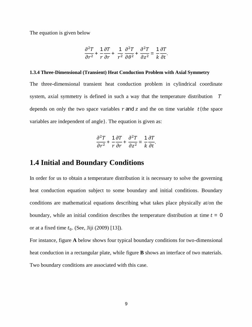
1.3.4 Three-Dimensional (Transient) Heat Conduction Problem with Axial Symmetry
The three-dimensional transient heat conduction problem in cylindrical coordinate
system, axial symmetry is defined in such a way that the temperature distribution 푇
depends on only the two space variables 푟 and 푧 and the on time variable 푡{the space
variables are independent of angle}. The equation is given as:
휕 푇휕푟
+1푟휕푇휕푟
+휕 푇휕푧
=1푘휕푇휕푡
.
1.4 Initial and Boundary Conditions
In order for us to obtain a temperature distribution it is necessary to solve the governing
heat conduction equation subject to some boundary and initial conditions. Boundary
conditions are mathematical equations describing what takes place physically at/on the
boundary, while an initial condition describes the temperature distribution at time 푡 = 0
or at a fixed time 푡 . (See, Jiji (2009) [13]).
For instance, figure A below shows four typical boundary conditions for two-dimensional
heat conduction in a rectangular plate, while figure B shows an interface of two materials.
Two boundary conditions are associated with this case.

10
Figure 1.1: Boundary and Interfacial Conditions
1.4.1 Specified Temperature
The specified temperature along the boundary is (0,푦) in figure A is 푇 . This temperature
can be uniform or can vary along 푦 as well as with time. Mathematically this condition
is expressed as
푇(0,푦, 푡) = 푇 .
1.4.2 Specified Heat Flux
The specified heat flux along boundary (퐿,푦) in figure A is 푞(퐿,푦, 푡). According to
Fourier’s law this condition is expressed as
푞(퐿,푦, 푡) = −푘휕푇(퐿,푦, 푡)
휕푥.
In particular, the boundary at (푥,푊) is thermally insulated in figure A. Thus, the
specified heat flux would now be
휕푇(푥,푊, 푡)휕푥
= 0.
a

11
1.4.3 Interface Condition
Figure B shows a composite wall of two materials with thermal diffusivities 푘 and 푘 .
For a perfect interface contact, the two temperatures must be the same at the interface.
Thus,
푇 (0,푦, 푡) = 푇 (0,푦, 푡).
Conservation of energy at the interface requires that the two fluxes be identical.
Application of Fourier’s law gives
푘휕푇 (0,푦, 푡)
휕푥= 푘
휕푇 (0,푦, 푡)휕푥
.
1.5 Solution of Heat Conduction Problem
To solve the heat conduction problem, that is, the given heat conduction partial
differential equation irrespective of the coordinate system and the boundary conditions
(or initial condition) means that finding the temperature distribution or temperature field
function that depends on various space parameters (such as 푥,푦, 푧 or 푟,휃, 푧 ) and on the
time variable that is consistent with the conditions defined on the boundary. In this
regard, several techniques are available with separation of variable method as the most
widely used method and then the integral transform methods. However, the boundary
conditions also play a very important role in choosing which method to be used. For
instance, while using the Fourier transform method, we put our concern on the nature of
the boundary conditions; on doing that, we determine whether to use Fourier Sine or
Fourier cosine method as sub-classes of Fourier transform method.

12
CHAPTER TWO
INTEGRAL TRANSFORMS AND WIENER-HOPF
TECHNIQUE
2.0 Introduction
In this chapter, we present the methodology to be followed in order to solve our intended
problems in chapters three and four. To solve our mixed boundary value problem, we use
the technique that is based upon the integral transforms. The transforms to be used are the
Laplace transform in the time variable and the Fourier transform in the space variables.
However, many problems of practical interest with our problem inclusive give rise to
singular integral equations defined in (0,∞) range which the above mentioned transforms
and others like Mellin transform do not allow the use of the convolution theorem thereby
rendering these transforms inapplicable. Thus, we present a method due to Wiener and
Hopf called Wiener-Hopf technique or method to solve such integral equations. Besides,
we also present the Modified Wiener-Hopf technique by Jones which simplifies the
difficulties faced in dealing with the integral equations by simply applying the technique
to the governing partial differential equation and its boundary conditions. Some theorems
are also presented.

13
2.1 Laplace Transform
The Laplace transform in the time variable 푡 is defied {whenever it exists} by
ℒ{푇(푡)} = 푇(푡)푒 푑푡 = 푇(푠), and (2.1)
Laplace inverse transform in the Laplace parameter 푠 is defined {whenever it exists} by
ℒ {푇(푠)} =1
2휋푖푇(푠)푒 푑푠 = 푇(푡). (2.2)
2.2 Fourier Transform
The Fourier transform is taken in one of the space variables. The transform and its
corresponding inverse are defined by
ℱ{푇(푥)} = 푇(푥)푒 푑푥 = 푇∗(훼), and (2.3)
ℱ {푇∗(훼)} =1
2휋푇∗(훼)푒 푑훼 = 푇(푥). (2.4)
If these integrals exist.

14
2.3 Fourier Transform of One-Sided Functions
We first introduce the one-sided functions due to their usefulness in the context of mixed
boundary value problems. We define {푇 (푥)} an upper (right) and {푇 (푥)} a lower (left)
half functions called one-sided functions as
푇 (푥) = 푇(푥), 푥 > 0 0, 푥 < 0 and 푇 (푥) = 0, 푥 > 0
푇(푥), 푥 < 0 .
Having defined the Fourier transform which is defined over (−∞,∞) range; we also need
to define the Fourier transform of the so-called one sided functions. That is, a function
defined only on a half-range.
So, the Fourier transform of 푇 (푥) would be:
ℱ{푇 (푥)} = 푇 (푥)푒 푑푥 = 푇 (푥)푒 푑푥 = 푇∗(훼). (2.5)
where, 훼 = 휎 + 푖휏, and 푇 (푥) = Ο(푒 ) as 푥 → ∞, i.e.
|푇 (푥)| ≤ 퐶 |푒 | 푎푠 푥 → ∞.
Then,
푇 (푥)푒 ( ) 푑푥 ≤ 퐶 푒 ( ) 푑푥.
Thus, ℱ{푇 (푥)} is defined as analytic function if 휏 > −푎.

15
Figure 2.1: Upper Half-Plane
In the same way, we define 푇∗(훼) as:
ℱ{푇 (푥)} = 푇 (푥)푒 푑푥 = 푇 (푥)푒 푑푥 = 푇∗(훼). (2.6)
where 훼 = 휎 + 푖휏, and 푇 (푥) = Ο(푒 ) as 푥 → −∞. i.e.
|푇 (푥)| ≤ 퐶 |푒 | 푎푠 푥 → −∞.
Then,
푇 (푥)푒 ( ) 푑푥 ≤ 퐶 푒( ) 푑푥
Thus, ℱ{푇 (푥)} is defined as analytic function if 휏 < 푎.

16
Figure 2.2: Lower Half-Plane
Hence,
푇∗(훼) = 푇(푥)푒 푑푥 = 푇 (푥)푒 푑푥 + 푇 (푥)푒 푑푥.
So that , 푇∗(훼) = 푇∗(훼) + 푇∗(훼). (2.7)
Where, 푇∗(훼) is an analytic function of 훼 if −푎 < 휏 < 푎
for 푇(푥) = Ο 푒 | | as |푥| → ∞. The region given by −푎 < 휏 < 푎 is called the strip
of analyticity, of 푇∗(훼).

17
2.4 Theorems
The theorems to be used in this work are listed and stated as follows
2.4.1 Additive Decomposition Theorem
Let 푓(훼) be an analytic function of 훼 = 휎 + 푖휏, regular in the strip 휏 < 휏 < 휏 , such
that |푓(휎 + 푖휏)| < 퐶|휎| ,푝 > 0, for |휎| → ∞, the inequality holding uniformly for all 휏
in the strip 휏 + 휀 ≤ 휏 ≤ 휏 − 휀, 휀 > 0. Then, for 휏 < 푐 < 휏 < 푑 < 휏 ;
푓(훼) = 푓 (훼) + 푓 (훼)
with
푓 (훼) =1
2휋푖푓(휁)휁 − 훼
푑휁 and 푓 (훼) = −1
2휋푖푓(휁)휁 − 훼
푑휁,

18
where 푓 (훼) is regular for all 휏 > 휏 and 푓 (훼) is regular for all 휏 < 휏 respectively.
[19]
2.4.2 Multiplicative Factorization Theorem
If 퐾(훼) satisfies the conditions of theorem above, which implies in particular that 퐾(훼)
is regular and non-zero in a strip 휏 < 휏 < 휏 , −∞ < 휎 < ∞ and 퐾(훼) → +1 as
휎 → ±∞ in the strip, then we can write
퐾(훼) = 퐾_(훼) 퐾 (훼)
with
퐾 (훼) = 푒푥푝 ∫ ( )푑휁 and 퐾 (훼) = 푒푥푝 − ∫ ( )푑휁 ,
where 퐾_(훼), and 퐾 (훼) are regular, bounded, and non-zero in 휏 > 휏 and 휏 < 휏 ,
respectively. [19]
2.4.3 Extended form of Liouville’s Theorem
If 푓(푧) is an entire function such that |푓(푧)| ≤ 푀|푧| as |푧| → ∞ where 푀, 푝 are
constants, then 푓(푧) is a polynomial pf degree less than or equal to [푝] where [푝] is the
integral part of 푝. [19]

19
2.4.4 Residue Theorem
Suppose 푓(푧) is analytic inside and on a simple closed contour 퐶 except for isolated
singularities at 푧 , 푧 , … , 푧 inside 퐶. Then
푓(푧) = 2휋푖 푅푒푠[푓(푧); 푧 ],
[29].
2.4.5 Infinite Product Theorem
Consider an entire function 퐾(훼) which
a). is an even function of 훼, that is 퐾(훼) = 퐾(−훼),
b). has simple zeros at 훼 = ±푖훼 ,푛 = 1, 2, …, and 훼 → 푎푛 + 푏, 푛 → ∞.
Then 퐾(훼) can be represented by either of the two forms
퐾(훼) =
⎩⎪⎨
⎪⎧ 퐾(0) (1 −
훼푖훼
)(1 + 훼푖훼
)
퐾(0) (1 − 훼푖훼
)푒 (1 + 훼푖훼
)푒
[23].

20
2.4.6 Jordan’s Lemma
Suppose we have a circular arc 퐶 with center 0; If 푚 > 0 and 푓(푧) = ( )( )
such
that degree of 푝 ≥ 1 + 푑푒푔푟푒푒 표푓 푞, then
lim→
푓(푧)푒± 푑푧 = 0
With if 푚 > 0: 퐶 is closed in the upper half plane
And if 푚 < 0: 퐶 is closed in the lower half plane. [23]
2.5 The Wiener-Hopf Equation
We describe the method by considering a singular integral equation that arises in integral
equation formulation of the mixed boundary value problems.
Consider the integral equation
푘(푥 − 휉)푓(휉)푑휉 = 휇푓(푥) + 푔(푥), 0 < 푥 < ∞ (2.8)
where 휇, 푔(푥) and 푓(푥) are given and wish to find 푓(푥), 0 < 푥 < ∞.
The first step is to extend the range of integration to infinite interval −∞ < 푥 < ∞ as
follows
푘(푥 − 휉)푓(휉)푑휉 = 휇푓(푥) + 푔(푥), 0 < 푥 < ∞ℎ(푥), −∞ < 푥 < 0 (2.9)

21
with
ℎ(푥) = 푘(푥 − 휉)푓(휉)푑휉
where
푓(푥) = 0; 0 < 푥 푔(푥) = 0; 0 < 푥ℎ(푥) = 0; 푥 > 0
.
So, we call the above functions 푓 (푥), 푔 (푥) and ℎ (푥) respectively. Thus, functions
푓 (푥) and 푔 (푥) which varnish for negative 푥 are said to be right-sided functions,
whereas, ℎ (푥) is a left-sided function. Therefore equation (2.9) can be rewritten as
푘(푥 − 휉)푓 (휉)푑휉 = 휇푓 (푥) + 푔 (푥) + ℎ (푥), −∞ < 푥 < ∞. (2.10)
We give some list the assumptions under which we will attempt to solve equation (2.11):
I. 푘(푥) = 0(푒 | |) as |푥| → ∞, 푐 > 0.
II. 푔(푥) = 0 푒 as 푥 → +∞,푑 < 푐.
The integral on the left-side exists if 푓(푥) is of exponential order at infinity with
exponential smaller than 푐. Thus we shall look for a solution 푓(푥) satisfying
III. 푓(푥) = 0 푒 as 푥 → +∞,푑 < 푐.
From I and III, it then follows that

22
IV. ℎ(푥) = 0(푒 | |) as 푥 → −∞.
And on taking the Fourier transform of equation (2.10) we get
푘∗(훼)푓∗(훼) = 휇푓∗(훼) + 푔∗ (훼) + ℎ∗ (훼). (2.11)
Hence, equation (2.11) is called the Wiener-Hopf equation, where the transforms are
defined and analytic in the following regions:
푘∗(훼) in the strip −푐 < Im(훼) < 푐;
푓∗(훼) in the upper half-plane Im(훼) > 푑 ;
푔∗ (훼) in the upper half-plane Im(훼) > 푑 ;
ℎ∗ (훼) in the lower half-plane Im(훼) < 푐.
If we let 푑 = max (푑 ,푑 ), then all the functions are valid in the strip 푑 < Im(훼) < 푐 of
analyticity. (see Stakgold [22] for more details).
2.6 Solution of the Wiener-Hopf Equation
We can rewrite equation (2.11) as
푓∗(훼) { 푘∗(훼) − 휇} − 푔∗ (훼) = ℎ∗ (훼). (2.12)
From equation (2.12), the function 푘∗(훼) − 휇 is neither positive nor negative function,
therefore we need to factorize it into two non-zero functions by the use of factorization
theorem 2.4.2. That is, we factorize it as:

23
푘∗(훼) − 휇 = 푘 (훼)푘 (훼)
Therefore, equation (2.12) becomes
푓∗(훼)푘 (훼) − 푔∗ (훼)푘 (훼) =
ℎ∗ (훼)푘 (훼) . (2.13)
In the same way, we notice from equation (2.13) that ∗ ( )
( ) is a mixed function;
therefore it needs to be decomposed by the use of additive decomposition theorem 2.4.1,
thus,
푔∗ (훼)푘 (훼) = 푚 (훼) + 푚_(훼).
Finally, equation (2.13) becomes
푓∗(훼)푘 (훼) − 푚∗ (훼) = ℎ∗ (훼)푘 (훼) + 푚∗ (훼) = 퐽(훼). (2.14 )
As the left hand side of the equation (2.14) is analytic in the upper half-plane while the
right hand side is analytic in the lower half-pane, both sides are equal in the common
strip; we conclude that these define an entire function 퐽(훼) by analytic continuation.
By an extended form of Liouville’s theorem 2.4.3, this analytic function is constant. In
most practical cases this constant can be evaluated to be zero by the asymptotic behavior
of the left or right hand side.

24
Thus, the unknown function in equation (2.14) is
푓∗(훼) =푚∗ (훼)푘 (훼) . (2.15)
Finally, on taking the Fourier inverse transform of equation (2.15), we simply get our
function 푓(푥) as
푓(푥) =1
2휋푚∗ (훼)푘 (훼) 푒 푑훼 . (2.16)
2.7 Modified Jones Method
In the modification due to D. S. Jones [15], the Wiener-Hopf functional equation is
derived directly from the boundary value problem rather than having to first reduce it to
the integral equation. To illustrate the main steps, we demonstrate the method by
considering an incoming acoustic wave incident on a rigid half-plane. We consider the
wave to be time harmonic but that is not a limitation as for the transient waves, we can
first apply the Laplace transform in time and then proceed. We thus consider
푢 + 푢 + 푘 푢 = 0, (2.17)
where 푢 is the diffracted wave given by 푢 = 푢 − 푢 , where 푢 is the velocity potential
and 푢 is the incident wave, and 푘 is the wave number having a positive imaginary part.
The following conditions apply:
25
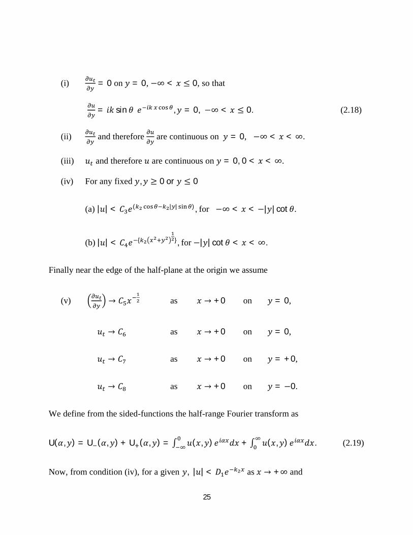
(i) = 0 on 푦 = 0, −∞ < 푥 ≤ 0, so that
= 푖푘 sin 휃 푒 ,푦 = 0, −∞ < 푥 ≤ 0. (2.18)
(ii) and therefore are continuous on 푦 = 0, −∞ < 푥 < ∞.
(iii) 푢 and therefore 푢 are continuous on 푦 = 0, 0 < 푥 < ∞.
(iv) For any fixed 푦,푦 ≥ 0 or 푦 ≤ 0
(a) |푢| < 퐶 푒( | | ), for −∞ < 푥 < −|푦| cot휃.
(b) |푢| < 퐶 푒 { }, for −|푦| cot휃 < 푥 < ∞.
Finally near the edge of the half-plane at the origin we assume
(v) → 퐶 푥 as 푥 → +0 on 푦 = 0,
푢 → 퐶 as 푥 → +0 on 푦 = 0,
푢 → 퐶 as 푥 → +0 on 푦 = +0,
푢 → 퐶 as 푥 → +0 on 푦 = −0.
We define from the sided-functions the half-range Fourier transform as
U(훼,푦) = U (훼,푦) + U (훼,푦) = ∫ 푢(푥,푦) 푒 푑푥 + ∫ 푢(푥,푦) 푒 푑푥. (2.19)
Now, from condition (iv), for a given 푦, |푢| < 퐷 푒 as 푥 → +∞ and

26
|푢| < 퐷 푒 as 푥 → −∞ where 퐷 ,퐷 are constants.
Thus, U is analytic for 휏 > −푘 , U is analytic for 휏 < 푘 cos휃, and U is analytic in the
strip −푘 < 휏 < 푘 cos휃.
Also,
|U| ≤ |U | + |U |.
If we now take the Fourier transform in 푥 to equation (2.17), we get
푑푈(훼,푦)
푑푦− 훾 푈(훼,푦) = 0, 훾 = (훼 − 푘 ) . (2.20)
More details on 훾 = (훼 − 푘 ) are explained in Nobel [19]. Thus, the solution of
equation (2.20) takes the form:
푈(훼,푦) = 퐴 (훼)푒 + 퐵 (훼)푒 , 푦 ≥ 0 퐴 (훼)푒 + 퐵 (훼)푒 , 푦 ≤ 0 ,
(2.21)
where 퐴 ,퐵 퐴 , and 퐵 are functions of 훼 and 푈 is discontinuous at 푦 = 0. Further, from
equation (2.20), the real part of 훾 is always positive in −푘 < 휏 < 푘 and therefore in
equation (2.21) we must take 퐵 = 퐴 = 0. From condition (ii), is continuous
across푦 = 0. Hence is continuous across 푦 = 0 and we can set
퐴 (훼) = −퐵 (훼) = 퐴(훼), say.

27
Hence
푈(훼,푦) = 퐴(훼)푒 , 푦 ≥ 0퐴(훼)푒 , 푦 ≤ 0.
(2.22)
Now, when a transform is discontinuous across 푦 = 0, we extend the notation by writing
for instance 푈(훼, +0) or 푈(훼,−0) to mean that the limit as 푦 tends to zero approached
from positive value of 푦 or approached from the left respectively. Thus, from condition
(ii), 푈 (훼, +0) = 푈 (훼,−0) = 푈 (훼, 0), and similarly for 푈 (훼, 0). Likewise from
condition (iii), 푈 (훼, +0) = 푈 (훼,−0) = 푈(훼, 0).
Thus, applying the definition above to equation (2.22), we get the following
푈 (훼, 0) + 푈 (훼, +0) = 퐴(훼), (2.23푎)
푈 (훼, 0) + 푈 (훼,−0) = −퐴(훼), (2.23푏)
푈 (훼, 0) + 푈 (훼, 0) = −훾퐴(훼). (2.23푐)
Eliminating 퐴(훼) in equation (2.33); adding equations (2.33a) and (2.33b) we get
2푈 (훼, 0) = −푈 (훼, +0) − 푈 (훼,−0). (2.24)
On subtracting equation (2.33b) from (2.33a) and eliminating 퐴(훼) between the resulting
equation and equation (2.33a), we obtain
푈 (훼, 0) + 푈 (훼, 0) = −12훾{푈 (훼, +0) − 푈 (훼,−0)}. (2.25)

28
Thus, from equation (2.25), 푈 (훼, 0) is known from condition (i) after evaluating it as
푈 (훼, 0) = 푖푘 sin 휃 푒 푒 푑푥 =푘 sin 휃
훼 − 푘cos휃. (2.26)
For simplicity, we let
푈 (훼, +0) − 푈 (훼,−0) = 2퐷 (훼) and 푈 (훼, +0) + 푈 (훼,−0) = 2푆 (훼), (2.27)
where 퐷 (훼) and 푆 (훼) represent the difference and sum of two functions respectively
that are both analytic for 휏 < 푘 cos휃.
Equations (2.24) and (2.25) become:
푈 (훼, 0) = −푆 (훼), (2.28)
푈 (훼, 0) +푘 sin휃
훼 − 푘cos휃= −훾퐷 (훼). (2.29)
Thus, equations (2.28) and (2.29) give the Wiener-Hopf functional equation with four
unknowns 푈 (훼, 0),푈 (훼, 0), 푆 (훼) and 퐷 (훼) that hold in the common strip of
analyticity −푘 < 휏 < 푘 cos휃.
Finally, to solve equations (2.28) and (2.29), we apply the same procedure discussed
above in section 2.6.

29
CHAPTER THREE
HEAT CONDUCTION IN A CIRCULAR HOLLOW
CYLINDER AMIDST MIXED BOUNDARY
CONDITIONS
3.0 Introduction
The heat conduction in circular cylinders is of interest in many engineering applications.
In case of a reactor, the circular cylinders containing radioactive source are cooled by
water. In such cases, part of the cylinder may be immersed in water giving rise to mixed
boundary conditions on the outer surface of the cylinder. In this chapter, we determine
the analytical solution of the transient heat conduction in a homogenous isotropic hollow
infinite cylinder that is subjected to different boundary conditions on the outer surface
while the inner surface temperature is kept at zero temperature throughout. Thus, the
dimensions of the hollow cylinder are −∞ < 푧 < ∞ in the axial direction and the
cylinder occupies 푎 < 푟 < 푏 where 푎 and 푏 are positive and 푎 ≠ 푏. We further assume
axial symmetry so that all field variables are independent of angle. The Jones’
modification method of the Wiener-Hopf technique is utilized due to the mixed nature of
the boundary conditions on the outer surface of the hollow cylinder.
30
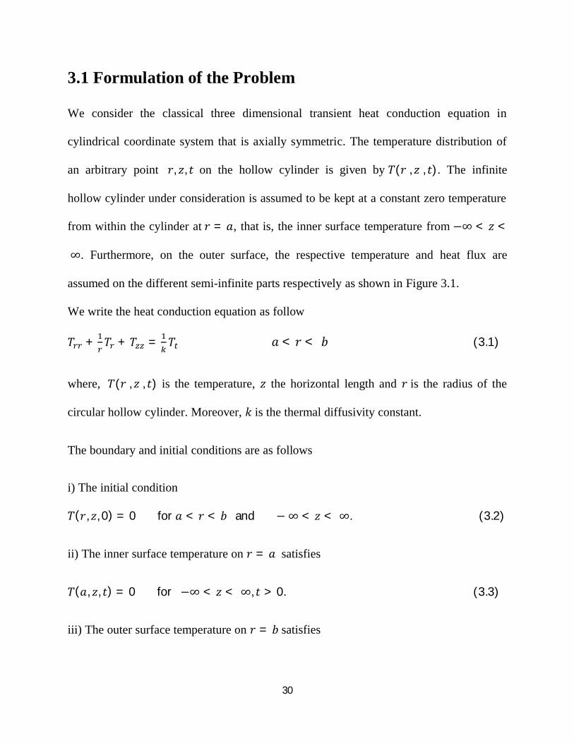
3.1 Formulation of the Problem
We consider the classical three dimensional transient heat conduction equation in
cylindrical coordinate system that is axially symmetric. The temperature distribution of
an arbitrary point 푟, 푧, 푡 on the hollow cylinder is given by 푇(푟 , 푧 , 푡). The infinite
hollow cylinder under consideration is assumed to be kept at a constant zero temperature
from within the cylinder at 푟 = 푎, that is, the inner surface temperature from −∞ < 푧 <
∞. Furthermore, on the outer surface, the respective temperature and heat flux are
assumed on the different semi-infinite parts respectively as shown in Figure 3.1.
We write the heat conduction equation as follow
푇 + 푇 + 푇 = 푇 푎 < 푟 < 푏 (3.1)
where, 푇(푟 , 푧 , 푡) is the temperature, 푧 the horizontal length and 푟 is the radius of the
circular hollow cylinder. Moreover, 푘 is the thermal diffusivity constant.
The boundary and initial conditions are as follows
i) The initial condition
푇(푟, 푧, 0) = 0 for 푎 < 푟 < 푏 and −∞ < 푧 < ∞. (3.2)
ii) The inner surface temperature on 푟 = 푎 satisfies
푇(푎, 푧, 푡) = 0 for −∞ < 푧 < ∞, 푡 > 0. (3.3)
iii) The outer surface temperature on 푟 = 푏 satisfies

31
푇(푏, 푧, 푡) = 푇 푒 , for 0 < 푧 < ∞, 푡 > 0; 푇 and 휆 > 0 are constants. (3.4)
iv) The heat flux on 푟 = 푏 is given by
푇 (푏, 푧, 푡) = 0 for −∞ < 푧 < 0, 푡 > 0. (3.5)
In solving the above system, we put 푇(푟, 푧, 푡) = 푒 푢(푟, 푧), { 푘 is the thermal
diffusivity, and 휇 is constant} in equation (3.1) to get
푢푟푟 + 1
푟푢푟 + 푢푧푧 + 휇 푢 = 0. (3.6)
Figure 3.1: Geometry of the problem

32
3.2 Wiener-Hopf Equation
We define the Fourier transform in 푧 and its corresponding inverse transform in 훼 {if
exist} as:
ℱ{푢(푧)} = ∫ 푢(푧)푒 푑푧 = 푢∗(훼), (3.7)
ℱ {푢∗(훼)} = ∫ 푢(훼)푒 푑훼 = 푢(푧). (3.8)
We also give the half range Fourier transforms as
∫ 푢(푧)푒 푑푥 = 푢∗ (훼), (3.9)
∫ 푢(푧)푒 푑푥 = 푢∗_(훼). (3.10)
We use the Fourier transform and half-range functions of Fourier transform described in
chapter 2, and write
푢∗(훼) = 푢∗ (훼) + 푢∗_(훼), (3.11)
푢(훼) = 0(푒 _ ) as 푧 → ∞ and 푢(훼) = 0(푒 ) as 푧 → −∞. Thus 푢∗ (훼) is an analytic
function of 훼 in the upper half-plane 휏 > 휏_, while 푢∗_(훼) is an analytic function of 훼 in
the lower half-plane 휏 < 휏 respectively. Thus, 푢∗(훼) defines an analytic function in the
common strip 휏_ < 휏 < 휏 with 휏 = 퐼푚(훼) where 훼 = 휎 + 푖휏.

33
Now, taking the Fourier transform in 푧 of equation (3.6), we obtain
푢∗ + 푢∗ + (휇 − 훼 )푢∗ = 0. (3.12)
Similarly taking the Fourier transform of the boundary conditions, we obtain
i) 푢∗(푎,훼) = 0, (3.13)
ii) 푢∗ (푏,훼) = 푖 , (3.14)
iii) 푢∗ (푏,훼) = 0. (3.15)
Solution of equation (14) is given by
푢∗(푟,훼) = 퐴 퐽 (푤푟) + 퐵 푌 (푤푟), (3.16)
where 퐽 (푤푟) and 푌 (푤푟) are Bessel functions of first and second kinds respectively.
Further, 푤(훼) denotes the square-root function
푤(훼) = 휇 − 훼 , (3.17)
which is defined in the complex 훼 −plane, with cuts along 훼 = 휇 to 훼 = 휇 + 푖∞ and
훼 = −휇 to 훼 = −휇 − 푖∞ such as 푤(0) = 휇 (see [12]).
Thus, from the boundary condition given in equation (3.13) we obtain
퐴 퐽 (푤푎) + 퐵 푌 (푤푎) = 0. (3.18)
Similarly from boundary conditions in equations (3.14) and (3.14) we get the following
respective equations
푢∗ (푏,훼) + 푖 = 퐴 퐽 (푤푏) + 퐵 푌 (푤푏), (3.19)
푢∗ (푏,훼) = −푤{퐴 퐽 (푤푏) + 퐵 푌 (푤푏)}. (3.20)

34
Therefore, solving for 퐵 from equation (3.18), as
퐵 = −퐴 ( )( )
,
and substituting it into equations (3.19) and (3.20) we get the following equations
푢∗ (푏,훼) + 푖 =( )
{ 푌 (푤푎)퐽 (푤푏) − 퐽 (푤푎)푌 (푤푏)}, (3.21)
푢∗ (푏,훼) = −푤 ( )
{푌 (푤푎) 퐽 (푤푏) − 퐽 (푤푎)푌 (푤푏)}. (3.22)
Hence, from equations (3.21) and (3.22), we get the Winer-Hopf equation given in
푢∗ (푏,훼) + 푖 = ( , , ) ( , , )
푢 (푏,훼), (3.23)
where,
푇 (푎, 푏,훼) = 푌 (푤푎)퐽 (푤푏) − 퐽 (푤푎)푌 (푤푏), (3.24푎)
푇 (푎, 푏,훼) = 푤{퐽 (푤푎)푌 (푤푏) − 푌 (푤푎) 퐽 (푤푏)}. (3.24푏)
For brevity sake, we write
푀(훼) =푇 (푎, 푏, 훼) 푇 (푎, 푏,훼) ,
that is,
푀(훼) = ( , , ) ( , , ) = ( ) ( ) ( ) ( )
{ ( ) ( ) ( ) ( )}. (3.25)
3.3 Solution of the Wiener-Hopf Equation
To solve the Wiener-Hopf equation (3.23), we use the factorization theorem in chapter 2
over 푀(훼) in equation (3.25) and factorize it into the product of 푀 (훼) and 푀 (훼) in

35
such a way that 푀 (훼) is analytic in the upper half-plane 휏 > 휏 and 푀 (훼) analytic in
the lower half-plane 휏 < 휏 respectively given theoretically as
푀 (훼) = exp ∫ ( )푑휁 , (3.26)
푀 (훼) = exp − ∫ ( )푑휁 . (3.27)
From equations (3.26) and (3.27), 푐 and 푑 are chosen within the analytic region
of 퐼푛 푀(휁). That is, 휏 < 푐 < 휏 < 푑 < 휏 .
Thus, 푀(훼) can be expressed using the infinite product factorization theorem [19] as
푀(훼) = 퐹훼 + 훼훼 + 훽
; 훼 ,훽 > 0,
where,
퐹 = 훽훼
{푌 (휇푎)퐽 (휇푏) − 퐽 (휇푎)푌 (휇푏)}휇{퐽 (휇푎)푌 (휇푏) − 푌 (휇푎) 퐽 (휇푏)}
.
That is,
푀(훼) = 퐹 ∏ = 푀 (훼)푀 (훼), (3.28)
where, ±푖훼 and ± 푖훽 are the simple zeros of 푇 (푎, 푏,훼) and 푇 (푎, 푏, 훼) respectively
for 푛 = 1,2, … Furthermore, the explicit functions of 푀 (훼) and 푀 (훼) are and given in
the Appendix I.

36
Finally, equation (3.23) becomes
푢∗ ( , )( ) + 푖
( ) ( ) = 푀 (훼)푢∗ (푏,훼). (3.29)
In the same way, the mixed term 푖( ) ( )
in equation (3.29) needs to be decomposed
either by the observation or through the use of additive decomposition theorem given in
chapter 2, given by
푖푇
(훼 + 푖휆)푀 (훼) = 푖푇
푀−(훼) − 푖푇
푀−(−푖휆),
where, 푖 푇푏( ) is an analytic function in the lower half-plane, 휏 < 휏 , while 푖 푇푏
( )
is an analytic function in the upper half-plane, 휏 > 휏 , respectively. Thus, equation
(3.29) becomes
( ) ( ) = 푖( ) ( ) − ( ) + 푖
( ) ( ). (3.30)
Thus, from equation (29), we obtain
( , )( ) + 푖
( ) ( ) − ( ) = − 푖 ( ) ( ) + 푀 (훼)푢 (푏,훼). (3.31)
As the left hand side of the equations (3.31) is analytic in the lower half-plane휏 < 휏 ,
while the right hand side is analytic in the upper half-pane, 휏 > 휏_, both sides are equal
in the common strip 휏 < 휏 < 휏 ; we conclude that these define an entire function by
analytic continuation. Thus, by an extended form of Liouville’s theorem 2.4.3, this
37
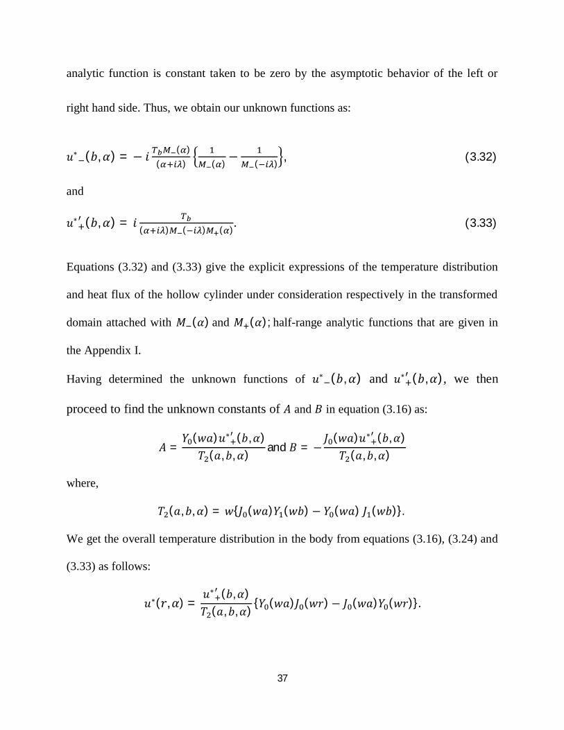
analytic function is constant taken to be zero by the asymptotic behavior of the left or
right hand side. Thus, we obtain our unknown functions as:
푢∗ (푏,훼) = − 푖 ( )( ) ( ) − ( ) , (3.32)
and
푢∗ (푏,훼) = 푖 ( ) ( ) ( ). (3.33)
Equations (3.32) and (3.33) give the explicit expressions of the temperature distribution
and heat flux of the hollow cylinder under consideration respectively in the transformed
domain attached with 푀 (훼) and 푀 (훼); half-range analytic functions that are given in
the Appendix I.
Having determined the unknown functions of 푢∗ (푏,훼) and 푢∗ (푏,훼), we then
proceed to find the unknown constants of 퐴 and 퐵 in equation (3.16) as:
퐴 =푌 (푤푎)푢∗ (푏,훼)
푇 (푎, 푏, 훼) and 퐵 = −퐽 (푤푎)푢∗ (푏,훼)
푇 (푎, 푏,훼)
where,
푇 (푎, 푏, 훼) = 푤{퐽 (푤푎)푌 (푤푏) − 푌 (푤푎) 퐽 (푤푏)}.
We get the overall temperature distribution in the body from equations (3.16), (3.24) and
(3.33) as follows:
푢∗(푟,훼) =푢∗ (푏,훼)푇 (푎, 푏,훼)
{푌 (푤푎)퐽 (푤푟) − 퐽 (푤푎)푌 (푤푟)}.

38
Where, 푢∗ (푏,훼) is already determined in equation (3.33). The Fourier inverse transform
would now be taken to obtain the temperature 푢(푟, 푧) and the flux 푢 (푟, 푧, ) in the whole
body in a space variable respectively. Hence, on taking the Fourier inverse transform, we
get the overall temperature distribution in the body from equations follows:
푢(푟, 푧) =1
2휋푢∗(푟,훼)푒 푑훼.
That is,
푢(푟, 푧) = ( )∫
( ) ( ) ( ) ( )( ) ( ) ( , , ) 푒 푑훼. (3.34)
Substituting the values of 푀 (훼) and 푇 (푎, 푏,훼) in equation (3.34) as expressed in the
Appendix I; we get
푢(푟, 푧) = ( , , ) ( )
∫( ) ( ) ( ) ( )
( )∏ { }∏ { } 푒 푑훼. (3.35)
Evaluating the integral in equation (3.35) using the residue calculus together with
Jordan’s lemma; in which the integrand is having simple poles at 훼 = −푖휆,−푖훼 and
푖훽 for 푛 = 1,2,3, … , we thus obtain;

39
푢(푟, 푧) =푇
퐹 푇 (푎, 푏, 0)푀 (−푖휆)
푌 (푤 푎)퐽 (푤 푟) − 퐽 (푤 푎)푌 (푤 푟)∏ {−푖휆 + 푖훼 }∏ {−푖휆 − 푖훽 }
푒
+푌 (푤 푎)퐽 (푤 푟) − 퐽 (푤 푎)푌 (푤 푟)
−푖훼 + 푖휆 ∏ {−푖훼 + 푖훼 } , ∏ −푖훼 − 푖훽
푒
−푌 (푤 푎)퐽 (푤 푟) − 퐽 (푤 푎)푌 (푤 푟)
푖훽 + 푖휆 ∏ {푖훽 + 푖훼 }∏ 푖훽 − 푖훽 ,푒 ,
(3.36)
where from equation(3.36), 푤 = 휇 + 휆 , 푤 = 휇 + 훼 and 푤 = 휇 + 훽 for
푗 = 1,2,3, . .. .
Thus, the overall temperature distribution of the hollow cylinder under the assumption
made earlier that 푇(푟, 푧, 푡) = 푒 푢(푟, 푧) is
푇(푟, 푧, 푡) =푇
퐹 푇 (푎, 푏, 0)푀 (−푖휆)
푌 (푤 푎)퐽 (푤 푟) − 퐽 (푤 푎)푌 (푤 푟)∏ {−푖휆 + 푖훼 }∏ {−푖휆 − 푖훽 }
푒
+푌 (푤 푎)퐽 (푤 푟) − 퐽 (푤 푎)푌 (푤 푟)
−푖훼 + 푖휆 ∏ {−푖훼 + 푖훼 } , ∏ −푖훼 − 푖훽
푒
−푌 (푤 푎)퐽 (푤 푟) − 퐽 (푤 푎)푌 (푤 푟)
푖훽 + 푖휆 ∏ {푖훽 + 푖훼 }∏ 푖훽 − 푖훽 ,푒 푒 .
(3.37)

40
3.4 Heat Flux on the Surface
In practical problems, we are more concerned about the heat flux rather than the
temperature distribution. Now, we define the heat flux by
푞 (푟, 푧, 푡) = −푘푒휕푢(푟, 푧)휕푟
, (3.38)
given that 푇(푟, 푧, 푡) = 푒 푢(푟, 푧).
Now, on taking the Fourier transform in 푧 of equation (3.38), we get
푞∗(푟,훼, 푡) = −푘푒휕푢∗(푟, 훼)
휕푟. (3.39)
Thus, substituting the heat flux obtained in equation (3.33) at 푟 = 푏 into equation
(3.39), we get
푞∗(푏, 훼, 푡) = −푘푒 푖푇
(훼 + 푖휆)푀 (−푖휆)푀 (훼). (3.40)
Now, taking the Fourier inverse transform ‘훼’, we get
푞 (푏, 푧, 푡) = −푘푒 푖푇2휋푀 (−푖휆)
푒(훼 + 푖휆)푀 (훼) 푑훼. (3.41)
Again, since 푀 (훼) is given in the Appendix I as: 푀 (훼) = 퐹 ∏ , where
±푖훼 and ±푖훽 are simple zeros of 푇 (푎, 푏, 훼) and 푇 (푎, 푏,훼) respectively.

41
Thus, equation (3.41) becomes
푞 (푏, 푧, 푡) = −푘푒 푖푇
2휋퐹 푀 (−푖휆)
∏ (훼 + 푖훽 ) 푒∏ (훼 + 푖훼 ) (훼 + 푖휆) 푑훼. (3.42)
Finally, applying the residue theorem by enclosing the contour in the lower half-plane,
the contributions of the poles as 훼 = −푖휆 and − 푖훼 for 푛 = 1,2,3 … give the overall heat
flux on the surface of the cylinder as
푞 (푏, 푧, 푡) =( )
∑∏ ( )
∏ ,− ( ) 푒 . (3.43)

42
CHAPTER FOUR
HEAT CONDUCTION IN A CIRCULAR CYLINDER
WITH GENERAL BOUNDARY CONDITIONS
4.0 Introduction
In chapter two, we introduced in details the Jones’ modification of the Wiener-Hopf
technique and there after used to solve a wave diffraction problem in two-dimension
subject to known mixed boundary conditions. There again, we determined the solution of
푢 + 푢 + 푘 푢 = 0 in 푦 ≥ 0, −∞ < 푥 < ∞,
such that 푢 represents the outgoing waves at infinity; also 푦 = 0, the mixed conditions
were given on 푢 = 0, 푥 > 0 and 푢 = 푖푘 sin휃 푒 . Furthermore, Nobel [19] stated
that the same problem can have generalized mixed boundary conditions, that is, on 푦 =
0; 푢 = 푓(푥) for 푥 > 0 and 푢 = 푔(푥) for 푥 < 0 respectively, where |푓(푥)| <
퐶 푒 as 푥 → ∞ and |푔(푥)| < 퐶 푒 as 푥 → −∞ with 퐶 and 퐶 are constants.
However, in this chapter, we intend to study and solve the heat conduction problem in an
infinite circular solid cylinder with finite radius when subjected to general mixed
boundary conditions on its outer surface. The generalized mixed boundary conditions
present on both the half-plane surfaces of the cylinder allow the use of the Jones’
modification of the Wiener-Hopf technique based on the application of Fourier

43
transforms. In this regard, the solution of the boundary value problem is aimed at
determining the temperature distribution and that of the heat flux of the problem under
consideration. Lastly, we determine an explicit analytical solution of the problem for
some special boundary conditions of interest.
4.1 Formulation of the Problem
We consider an infinite cylindrical rod of uniform cross section and finite radius 푟. The
cylinder is assumed to have the general mixed boundary conditions on the boundary; that
is, the temperature is given to by 푓(푟, 푧, 푡 ) in −∞ < 푧 < 0 while 푔(푟, 푧, 푡) represents the
heat flux in 0 < 푧 < ∞ as shown in Figure 4.1. The temperature 푇 in the cylinder
satisfies the governing equation
푇 +1푟푇 +
1푟푇 + 푇 =
1푘푇 (4.1)
and further assume that the heat conduction is axially symmetry, so that equation (4.1)
becomes
푇 +1푟푇 + 푇 =
1푘푇 (4.2)
where 푘 is the thermal diffusivity, expressed as 푘 = with 휐 thermal conductivity,
휌 density and 푐 specific heat constant all depending on the material. The initial and
boundary conditions are as follows

44
(i) The initial condition
푇(푟, 푧, 푡) = 0; 푎푡 푡 = 0. (4.3)
(ii) The temperature on 푧 < 0,
푇(푟, 푧, 푡) = 푓(푟, 푧, 푡 ); −∞ < 푧 < 0, 0 ≤ 푟 ≤ 푎. (4.4)
(iii) The heat flux on 푧 > 0,
푇 (푟, 푧, 푡) = 푔(푟, 푧, 푡); 0 < 푧 < ∞, 0 ≤ 푟 ≤ 푎. (4.5)
(iv) The continuity condition at 푧 = 0,
푇 (푟, 푧, 푡) = 푇 (푟, 푧, 푡); 푎푡 푧 = 0. (4.6)
In addition, the functions 푓(푟, 푧, 푡 ) and 푔(푟, 푧, 푡) are assumed to be of exponential order
as |푧| turns ∞.

45
Figure 4.1: Geometry of the problem
4.2 Wiener-Hopf Equation
The Laplace transform in the time variable 푡 and its inverse transform in 푠 are defined {if
exist} by:
ℒ{푇(푡)} = 푇(푡)푒 푑푡 = 푇(푠) (4.7)
and
ℒ {푇(푠)} =1
2휋푖 푇(푠)푒 푑푠 = 푇(푡) (4.8)
In the same way, we define the Fourier transform in 푧 and its corresponding inverse
Fourier transform in 훼 {if exist} by:
ℱ{푇(푧)} = 푇(푧)푒 푑푧 = 푇∗(훼) (4.9)

46
and
ℱ {푇∗(훼)} =1
2휋 푇∗(훼)푒 푑훼 = 푇(푧) (4.10)
with 훼 = 휎 + 푖휏.
Moreover, we also introduce the half range Fourier transforms as
푇(푧)푒 푑푧 = 푇∗(훼) (4.11)
and
푇(푧)푒 푑푧 = 푇∗(훼) (4.12)
So that,
푇∗(훼) = 푇∗(훼) + 푇∗(훼), (4.13)
푇(푧) = 0(푒 _ ) as 푧 → ∞ and 푇(푧) = 0(푒 ) as 푧 → −∞. Thus 푇∗(훼) is an analytic function of
훼 in the upper half-plane 휏 > 휏_, while 푇∗(훼) is an analytic function of 훼 in the lower half-plane
휏 < 휏 respectively. Thus, 푇∗(훼) defined an analytic function in the common strip 휏_ < 휏 < 휏
with 휏 = 퐼푚(훼).
We now take the Laplace transform in 푡 and Fourier transform in 푧 of equation (4.2) to
get
푇∗ +1푟푇∗ − 훼 +
푠푘푇∗ = 0. (4.14)
The transformed boundary conditions are given by
(i) 푇∗(푟,훼, 0) = 0, (4.15) (ii) 푇∗(푎,훼, 푠) = 푓∗(푎,훼, 푠), (4.16)
(iii) 푇∗ (푎,훼, 푠) = 푔∗ (푎,훼, 푠), (4.17)
(iv) 푇∗(푟, 0, 푠) = 푇∗(푟, 0, 푠). (4.18)
47
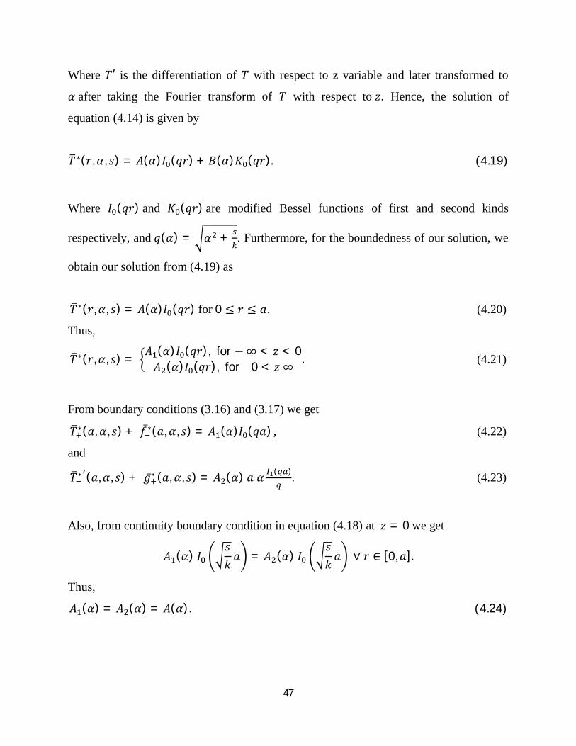
Where 푇′ is the differentiation of 푇 with respect to z variable and later transformed to
훼 after taking the Fourier transform of 푇 with respect to 푧. Hence, the solution of
equation (4.14) is given by
푇∗(푟,훼, 푠) = 퐴(훼)퐼 (푞푟) + 퐵(훼)퐾 (푞푟). (4.19)
Where 퐼 (푞푟) and 퐾 (푞푟) are modified Bessel functions of first and second kinds
respectively, and 푞(훼) = 훼 + . Furthermore, for the boundedness of our solution, we
obtain our solution from (4.19) as
푇∗(푟,훼, 푠) = 퐴(훼)퐼 (푞푟) for 0 ≤ 푟 ≤ 푎. (4.20)
Thus,
푇∗(푟,훼, 푠) = 퐴(훼)퐼 (푞푟), for −∞ < 푧 < 0퐴 (훼)퐼 (푞푟), for 0 < 푧 ∞ . (4.21)
From boundary conditions (3.16) and (3.17) we get
푇∗(푎, 훼, 푠) + 푓∗(푎, 훼, 푠) = 퐴 (훼)퐼 (푞푎) , (4.22)
and
푇∗ (푎,훼, 푠) + 푔∗ (푎, 훼, 푠) = 퐴 (훼) 푎 훼 ( ). (4.23)
Also, from continuity boundary condition in equation (4.18) at 푧 = 0 we get
퐴 (훼) 퐼푠푘푎 = 퐴 (훼) 퐼
푠푘푎 ∀ 푟 ∈ [0,푎].
Thus,
퐴 (훼) = 퐴 (훼) = 퐴(훼). (4.24)

48
Thus, equations (4.22) and (4.23) become
푇∗(푎, 훼, 푠) + 푓∗(푎, 훼, 푠) = 퐴(훼)퐼 (푞푎), (4.25)
and
푇∗ (푎,훼, 푠) + 푔∗ (푎, 훼, 푠) = 퐴(훼)푎 훼 ( ). (4.26)
From equations (4.24) and (4.26), we get the Wiener-Hopf equation given by
푇∗ (푎,훼, 푠) + 푔∗ (푎, 훼, 푠) = ( )( )
푇∗(푎,훼, 푠) + 푓∗(푎,훼, 푠) . (4.27)
4.3 Solution of the Wiener-Hopf Equation
In equation (4.27), the mixed term
푎훼 퐼 (푞푎)푞퐼 (푞푎) =
푎푖훼
퐽 (푖푞푎)푞퐽 (푖푞푎),
is denoted by 퐾(훼). {Note that 퐼 (푧) = 푖 퐽 (푖푧) as stated in chapter 1}.
We then factorize 퐾(훼) being a product of two meromorphic functions using
factorization theorem 2.4.2 as
퐾(훼) =푎 훼 퐼 (푞푎)푖 푞 퐼 (푞푎) = 퐾 (훼)퐾 (훼) (4.28)
(see Mittra and Lee [18] and Nobel [19]). Where 퐾 (훼) and 퐾 (훼) are analytic in the
upper and lower half planes respectively. The expression for 퐾 (훼) and 퐾 (훼) are given
in Appendix II in equations 퐷 and 퐷 respectively. Thus, equation (4.27) becomes
푇∗ (푎,훼, 푠)퐾 (훼) +
푔∗ (푎,훼, 푠)퐾 (훼) = 퐾 (훼)푇∗(푎,훼, 푠) + 퐾 (훼)푓∗(푎,훼, 푠). (4.29)
Again, decomposing the mixed terms in equation (4.29) using additive decomposition
theorem 2.4.1 we get as follows

49
푀(훼) =푔∗ (푎,훼, 푠)퐾 (훼) − 퐾 (훼)푓∗(푎,훼, 푠) = 푀 (훼) + 푀 (훼), (4.30)
where 푀 (훼) and 푀 (훼) are given to be
푀 (훼) =1
2휋푖푔∗ (푎, 휁, 푠)퐾 (휁) − 퐾 (휁)푓∗(푎, 휁, 푠)
1휁 − 훼
푑휁 , (4.31)
and
푀 (훼) = −1
2휋푖푔∗ (푎, 휁, 푠)퐾 (휁) − 퐾 (휁)푓∗(푎, 휁, 푠)
1휁 − 훼
푑휁 , (4.32)
respectively, where 푐 and 푑 are in the analytic region.
That is, 휏− < 푐 < 퐼푚(훼) < 푑 < 휏+. Finally, equation (4.30) becomes
푇∗ (푎,훼, 푠)퐾 (훼) + 푀 (훼) = 퐾 (훼)푇∗(푎,훼, 푠) −푀 (훼). (4.33)
Equation (4.33) defines an entire function in the whole 훼 − 푝푙푎푛푒 by analytic
continuation. In which the left hand side is analytic in the lower half-plane 휏 < 휏+, while
the right hand side is analytic in the upper half plane 휏 > 휏_ respectively. In addition,
both sides can be shown to be zero by the extended form of Liouville’s theorem 2.4.3
as 훼 → ±∞.
Thus, our unknown functions are found to be:
푇∗(푎,훼, 푠) =푀 (훼)퐾 (훼) , (4.34)
and
푇∗ (푎,훼, 푠) = −푀 (훼)퐾 (훼). (4.35)
We note that 퐾 (훼) and 퐾 (훼) are given by
퐾 (훼) =√푎√푖
퐿 (훼)푃 (훼),
퐾 (훼) =√푎√푖
훼퐿 (훼)푃 (훼),
and their explicit details are given in Appendix II in equations 퐷 and 퐷 , while 푀 (훼)
and 푀 (훼) are given by equations (4.31) and (4.32) in terms of known functions

50
respectively. Equations (4.34) and (4.35) can be then used together with (4.25) and (4.26)
to determine the overall temperature distribution in the transformed domain as
푇∗(푟,훼, 푠) =푇∗(푎,훼, 푠) + 푓∗(푎,훼, 푠)
퐼 (푞푎) 퐼 (푞푟).
The inverse Laplace transform and the inversion Fourier transform can then be taken to
obtain the temperature distribution 푇(푟, 푧, 푡) and the heat flux 푇푧(푟, 푧, 푡) respectively.
Hence, on taking these inversions we got the overall temperature distribution of the body
under consideration as follows:
푇(푟, 푧, 푡) =1
4휋 푖푇∗(푎,훼, 푠) + 푓∗(푎,훼, 푠)
퐼 (푞푎)퐼 (푞푟) 푒 푒 푑푠 푑훼 . (4.36)
4.4 Evaluation of the Temperature Distribution & Heat Flux
in Some Special Cases
Here, we intend to consider some boundary conditions specified on the outer surface of
the cylinder under consideration. That is, we consider a special case of transient heat
conduction, that is, the steady periodic heat conduction of the type
푇(푟, 푧, 푡) = 푇(푟, 푧) 푒 ,
where 휔 is the angular frequency. However, to determine the explicit analytical solutions
of the temperature distribution and the heat flux, we use the method of transforming a
transient heat conduction problem to a steady state problem suggested by Nobel [19].
That is, we transform the Laplace transform parameter 푠 to 푖휔 in the above equations
(4.31), (4.32), (4.34) and (4.35) respectively and also in 퐾 (훼) and 퐾 (훼) functions
given in the Appendix II respectively.
51
4.4.1 Case I
In case I, we assume the boundary conditions of the type
푇(푟, 푧, 푡) = 푇 , 푧 < 0 푎푛푑 푇 (푟, 푧, 푡) = 0, 푧 > 0 at 푟 = 푎 (4.37)
Transforming the boundary conditions after taking Laplace transform in t and Fourier
transform in z we get,
푇∗(푎, 훼, 푠) = and 푇∗ (푎, 훼, 푠) = 0, (4.38)
where 푇_ and 푇 ′ are the temperature distribution for 푧 < 0 and is the heat flux for
푧 > 0 at 푟 = 푎 respectively, and the prime stands for the derivative with respect to z.
Here, we use the method by Nobel [19] of transforming 푠 to 푖휔 in the equation (4.38),
that is, 푠 ↔ 푖휔, we get
푇∗(푎, 훼) = − and 푇∗ (푎,훼) = 0 (4.39)
So, on substituting the above transformed boundary conditions into equations (4.31) and
(4.32), we get
푀 (훼) =푇
2휋푖√푎휔√푖
퐿 (휁)휁(휁 − 훼)푃 (휁)푑 휁, (4.40)
and
푀 (훼) = −푇
2휋푖√푎휔√푖
퐿 (휁)휁(휁 − 훼)푃 (휁)푑 휁, (4.41)
where, 푃 (휁) = 퐽 (푖 푎)∏ (1 + ) and 퐿 (휁) = 퐽 (푖 푎)∏ (1 + ).

52
Thus, to evaluate the integrals in equations (4.40) and (4.41); we examine the simple
poles there present and make use of the complex residue calculus considering the
contours of integration closed in the upper half-plane by a semi-circle for both 푀 (훼)
and 푀 (훼) as evaluated below:
For 푀 (훼); we have simple poles at 휁 = 0, 휁 = 훼 and 휁 = −푖훼 = 훽 for 푃 (휁), where
훼 = 푖 , + for 푚 = 1, 2, … and 푗 , are the zeros of Bessel function of first
kind of order zero (see Appendix III).
Hence, equation (4.40) is evaluated below after closing the contour in the upper half-
plane such that all the poles lie inside, {휏 < 푐 < 푑} as:
푀 (훼) =푇 √푎휔√푖
퐴훼 − 훽
+퐿 (훼)훼푃 (훼) −
퐿 (0)훼푃 (0) , (4.42)
where, 퐴 = ( )( )
.
Similarly, for 푀 (훼), we have simple poles at 훽 ,훽 , . . ., 푘 ≪ 푚. Where 훽 ′푠 are
above the line −∞ + 푖푑 to ∞ + 푖푑 as such those 푐 < 푑 < 휏 . Thus, equation (4.41) is
evaluated as:
푀 (훼) =푇 √푎휔√푖
푩풌
훼 − 훽, (4.43)
where 푩풌 = ( )( )
.

53
4.4.1.1 Evaluation of the Temperature Distribution
To determine the temperature distribution on the surface of the cylinder at 푟 = 푎 for
푧 > 0 having determined the explicit function of 푀 (훼) in equation (4.42); we get the
following formula from equation (4.34):
푇∗(훼) =푀 (훼)퐾 (훼),
where
퐾 (훼) =√푎√푖
퐿 (훼)푃 (훼)
Thus, our transformed temperature for 푧 > 0 from equations (4.34) and (4.42) and after
using the expression of 퐾 (훼) we obtain:
푇∗(푎, 훼) =푇휔
퐴푃 (훼)
(훼 − 훽 )퐿 (훼) +1훼−
퐿 (0)푃 (훼)훼푃 (0)퐿 (훼) . (4.44)
Now, to evaluate the temperature distribution for 푧 > 0, in z-variable; we take the Fourier
inverse transform of equation (4.44) with respect to z as
푇 (푎, 푧) =푇휔
12휋
퐴푃 (훼)
(훼 − 훽 )퐿 (훼) +1훼−
퐿 (0)푃 (훼)훼푃 (0)퐿 (훼) 푒 푑훼. (4.45)
Here, evaluation of equation (4.45) follows the same procedure applied to equations
(4.40) and (4.41), that is, via residue calculus.

54
Equation (4.45) has simple poles at 훼 = 0, 훼 = 훽 for 푚 = 1,2, … and
훼 = −푖훼 = 훽 for 퐿 (훼), where 훼 = 푖 , + for 푛 = 1, 2, … and
훽 = , + for 푚 = 1,2, … with 푗 , and 푗 , are the zeros of Bessel function of
first kind of order zero and order one respectively.
So, from equation (4.45), we apply Jordan’s lemma 2.4.6 as follows:
For 푧 > 0; we close the contour in the lower half-plane and since there is no pole in the
closed contour, then
푇 (푎, 푧) = 0 for 푧 > 0. (4.46)
For 푧 < 0; we close the contour in the upper half-plane, but in such a way that 훼 = 0
would lie in the upper half-plane (i.e. would be inside the semi-circle). Thus, we get
푇 (푎, 푧) =
푖 ∑ 퐴 푒 + ∑ 퐴 ( )( )
푒, −∑ ( ) ( )( ) ( )
푒 ,
for, 푧 < 0 (4.47)
where, 퐴 =
( ).
Thus the overall temperature distribution is obtained by adding equations (4.46) and
(4.47) as
푇 (푎, 푧) =
푖 ∑ 퐴 푒 + ∑ 퐴 ( )( )
푒푛=1,푛≠푗 −∑ ( ) ( )( ) ( )
푒
(4.48)

55
Hence, to regain the time parameter in the temperature distribution, we get from our
earlier assumption that
푇 (푎, 푧, 푡) =
푇휔 푖 퐴
푃 훽퐿 훽
푒 + 퐴푃 (훽 )
훽 − 훽 퐿 (훽 )푒
,
−퐿 (0)푃 (훽 )훽 푃 (0)퐿 (훽 ) 푒 푒 .
(4.49)
4.4.1.2 Evaluation of the Heat Flux
The heat flux of the cylinder on 푟 = 푎 for 푧 < 0 is to be determined from equation (4.35)
given that the heat flux on 푧 > 0 is zero from equation (4.37); as
푇∗ (푎,훼) = −푀 (훼)퐾 (훼),
where
퐾 (훼) =√푎√푖
훼퐿_(훼)푃_(훼)
Thus, we get the heat flux function in the transformed domain for 푧 < 0 from equations
(4.37) and (4. 43) and also by the use of 퐾 (훼) function as:
푇∗ (푎,훼) = −푇 푎휔푖
퐵훼 − 훽
훼퐿( )
푃( ). (4.50)
And on taking the Fourier inversion transform in z, we obtain:
푇∗ (푎, 푧) = −푇 푎휔푖
12휋푖
퐵훼퐿( )
(훼 − 훽 )푃( ) 푒 푑훼 . (4.51)
56
So, we apply Jordan’s lemma 2.4.6 as follow to evaluate equation (4.51) as follows:
For 푧 > 0, we close the contour in the lower half-plane with simple poles at 훼 = −훽 ,
푚 = 1,2, … we obtain
푇∗ (푎, 푧) =푇 푎휔
푩풋훽 퐿_(−훽 )
(훽 + 훽 )푃′_(−훽 )푒 , 푧 > 0 (4.52)
Similarly, for 푧 < 0, we close the contour in the upper half-plane with the simple poles at
훼 = 훽 , 푘 = 1,2, … we obtain
푇∗ (푎, 푧) = −푇 푎휔
푩풋훽 퐿 훽푃 훽
푒 , 푧 < 0 (4.53)
Thus, the overall heat flux for 푧 < 0 is the summation of equations (4.52) and (4.53) as
푇∗ (푎, 푧) = −푇 푎휔
푩풋훽 퐿 훽푃 훽
푒 − 푩풋훽 퐿 (−훽 )
훽 + 훽 푃 (−훽 )푒 (4.54)
where 푩 =( )
.
Also to regain the time variable from our assumption, equation (4.54) for heat flux is:
푇∗ (푎, 푧, 푡) = −푇 푎휔
푩풋훽 퐿 훽푃 훽
푒 − 푩풋훽 퐿 (−훽 )
훽 + 훽 푃 (−훽 )푒 푒 .
(4.55)

57
4.4.2 Case II
We consider the boundary conditions of the type:
푇(푟, 푧, 푡) = 푇 푒 , 휆 > 0, 푧 < 0 and 푇 (푟, 푧, 푡) = 0, 푧 > 0 at 푟 = 푎. (4.56)
So, transforming the boundary conditions after taking Laplace transform in t and Fourier
transform in z we get,
푇∗(푎, 훼, 푠) =( )
and 푇∗ (푎,훼, 푠) = 0, (4.57)
where 푇_ and 푇 ′ are the temperature distribution for 푧 < 0 and the heat flux for 푧 > 0
at 푟 = 푎 respectively, whereas the prime {′} stands for the derivative of 푇 with respect
to z.
Here, we use the method by Nobel [19] of transforming 푠 to 푖휔 in the equation (4.56),
that is, 푠 ↔ 푖휔, we get
푇∗(푎, 훼) = −( )
and 푇∗ (푎, 훼) = 0. (4.58)
So, on substituting the above transformed boundary conditions into equations (4.31) and
(4.32), we get
푀 (훼) =푇
2휋푖√푎휔√푖
퐿 (휁)(휁 − 푖휆)(휁 − 훼)푃 (휁)푑 휁 (4.59)
and
푀 (훼) = −푇
2휋푖√푎휔√푖
퐿 (휁)(휁 − 푖휆)(휁 − 훼)푃 (휁) 푑 휁. (4.60)

58
Where 푃 (휁) = 퐽 (푖 푎)∏ (1 + ) and 퐿 (휁) = 퐽 (푖 푎)∏ (1 + ).
Thus, to evaluate the integrals in equations (4.59) and (4.60); we examine the simple
poles there present and make use of the complex residue calculus considering the
contours of integration.
For 푀 (훼); we have simple poles at 휁 = 푖휆, 휁 = 훼 and 휁 = −푖훼 = 훽 for 푃 (휁),
where 훼 = 푖 , + for 푚 = 1, 2, … and 푗 , are the zeros of Bessel function of
first kind of order zero.
Hence, equation (4.59) is evaluated using the method as in above as
푀 (훼) =푇 √푎휔√푖
퐴훼 − 훽
+퐿 (훼)
(훼 − 푖휆)푃 (훼) −퐿 (푖휆)
(훼 − 푖휆)푃 (푖휆) , (4.61)
where 퐴 = ( )( ) ( )
.
Similarly for 푀 (훼); we have simple poles at 훽 ,훽 , . . ., 푘 ≪ 푚. Where 훽 ′푠 are
above the line −∞ + 푖푑 to ∞ + 푖푑 as given in the above. Thus,
푀 (훼) =푇 √푎휔√푖
퐵훼 − 훽
, (4.62)
where 퐵 = ( )( ) ( )
.
59
4.4.2.1 Evaluation of the Temperature Distribution
To determine the temperature distribution on the surface of the cylinder at 푟 = 푎 for
푧 > 0 having determined the explicit function of 푀 (훼) in equation (4.61); we got the
following formula from equation (4.34):
푇∗(훼) =푀 (훼)퐾 (훼),
where
퐾 (훼) =√푎√푖
퐿 (훼)푃 (훼)
Thus, our temperature equation in the transformed domain for 푧 > 0 is derived from
equations (4.34) and (4.61) and indeed after using the expression of 퐾 (훼) as follows
푇∗(푎,훼) =푇휔
퐴푃 (훼)
(훼 − 훽 )퐿 (훼) +1
훼 − 푖휆−
퐿 (푖휆)푃 (훼)(훼 − 푖휆)푃 (푖휆)퐿 (훼) . (4.63)
Now, to evaluate the temperature distribution for 푧 > 0, in z-variable; we take the Fourier
inverse transform of equation (4.63) with respect to z as
푇 (푎, 푧) = ∫ ∑ 퐴 ( )( ) ( ) + − ( ) ( )
( ) ( ) ( ) 푒 푑훼.
(4.64)
Here, evaluation of equation (4.64) follows the same procedure applied to equations
(4.59) and (4.60), that is, via residue calculus.
Equation (4.64) has simple poles at 훼 = 푖휆, 훼 = 훽 for 푚 = 1,2, … and

60
훼 = −푖훼 = 훽 for 퐿 (훼), where 훼 = 푖 , + for 푛 = 1, 2, … and
훽 = , + for 푚 = 1,2, … with 푗 , and 푗 , the zeros of Bessel function of
first kind of order zero and order one respectively.
So, from equation (4.64), we apply Jordan’s lemma as follow: for 푧 > 0; we close the
contour in the lower half-plane and since there is no pole in the closed contour, then
푇 (푎, 푧) = 0 for 푧 > 0. (4.65)
For 푧 < 0; we close the contour in the upper half-plane, but in such a way 훼 = 푖휆 would
lie in the upper half-plane (i.e. would be inside the semi-circle). Thus, we get
푇 (푎, 푧) =
푖 ∑ 퐴 푒 + ∑ 퐴 ( )( ) ( )
푒, − ∑ ( ) ( )( ) ( ) ( )
푒
for, 푧 < 0 (4.66)
where 퐴 =( ) ( )
.
Thus, the overall temperature distribution is obtained by adding equations (4.65) and
(4. 66) as
푇 (푎, 푧) =
푖 ∑ 퐴 푒 + ∑ 퐴 ( )( ) ( )
푒, − ∑ ( ) ( )( ) ( ) ( )
푒
(4.67)
Hence, to regain the time parameter in the temperature distribution, we get from our
earlier assumption that

61
푇 (푎, 푧, 푡) =푇표휔푖 퐴푗
푃+ 훽푗
퐿+ 훽푗푒−푖훽푗푧 + 퐴푗
푃+ 훽푛(훽푛 − 훽푗)퐿+
′ 훽푛푒−푖훽푛푧
∞
푛=1,푛≠푗
∞
푗=1
−퐿+(푖휆)푃+ 훽푛
(훽푛 − 푖휆)푃+(푖휆)퐿+′ 훽푛
∞
푛=1
푒−푖훽푛푧 푒
(4.68)
4.4.2.2 Evaluation of the Heat Flux
The heat flux for 푧 < 0 at 푟 = 푎 as it is given to be zero on the other side by equation
(4.56) is to be determined from equation (4.35) given by
푇∗ (푎,훼) = −푀 (훼)퐾 (훼),
where,
퐾 (훼) =√푎√푖
훼퐿_(훼)푃_(훼)
Thus, we get the heat flux function in the transformed domain for 푧 < 0 from equations
(4.57) and (4.62) and also by the use of 퐾 (훼) function as:
푇∗ (푎, 훼) = −푇 푎휔푖
퐵훼 − 훽
훼퐿_(훼)푃_(훼). (4.69)
And on taking the Fourier inversion transform in z, we obtain:
푇∗ (푎, 푧) = −푇 푎휔푖
12휋푖
퐵훼퐿 (훼)
(훼 − 훽 )푃 (훼) 푒 푑훼 (4.70)
So, we apply Jordan’s lemma to evaluate equation (4.70) as follows: for 푧 > 0, we close
the contour in the lower half-plane with simple poles at 훼 = −훽 ,푚 = 1,2, … we obtain

62
푇∗ (푎, 푧) =푇 푎휔
푩풋훽 퐿_(−훽 )
(훽 + 훽 )푃′_(−훽 )푒 , 푧 > 0 (4.71)
Similarly, for 푧 < 0, we close the contour in the upper half-plane with the simple poles at
훼 = 훽 , 푘 = 1,2, … we obtain
푇∗ (푎, 푧) = −푇 푎휔
푩풋훽 퐿 훽푃 훽
푒 , 푧 < 0 (4.72)
Thus, the overall heat flux for 푧 < 0 is the summation of equations (4.71) and (4.72) as
푇∗ (푎, 푧) = −푇 푎휔
푩푗
훽푗퐿− 훽푗
푃−′ 훽푗푒−푖훽푗푧 − 푩푗
훽푚퐿_(−훽푚) (훽푚 + 훽푗)푃′_(−훽푚)
푒푖훽푚푧∞
푚=1
(4.73)
where 푩풋 =( ) ( )
.
Thus, to regain the time variable from our assumption, equation (4.73) for heat flux is:
푇∗ (푎, 푧, 푡) = −푇 푎휔
푩푗
훽푗퐿− 훽푗
푃−′ 훽푗푒−푖훽푗푧 − 푩푗
훽푚퐿_(−훽푚)
훽푚 + 훽푗 푃′_(−훽푚)푒푖훽푚푧
∞
푚=1
푒 .
(4.74)
4.4.3 Case III
In case III, we consider the boundary conditions of the form:
푇(푟, 푧, 푡) = 푇 푒 ,휇 > 0 , 푧 < 0 and 푇 (푟, 푧, 푡) = 0, 푧 > 0 at 푟 = 푎 (4.75)
So, transforming the boundary conditions after taking Laplace transform in t and Fourier
transform in z we get,
63
푇∗(푎, 훼, 푠) =( )
and 푇∗ (푎,훼, 푠) = 0, (4.76)
where 푇_ and 푇 ′ are the temperature distribution for 푧 < 0 and is the heat flux for
푧 > 0 at 푟 = 푎 respectively, and the prime stands for the derivative with respect to z.
Here, we 푠 to 푖휔 in the equation (4.76), so that:
푇∗(푎, 훼) = −( )
and 푇∗ (푎,훼) = 0. (4.77)
So, on substituting the above transformed boundary conditions into equations (4.31) and
(4.32), we get
푀 (훼) =푇
2휋푖√푎
(휔 − 푖휇)√푖퐿 (휁)
휁(휁 − 훼)푃 (휁)푑 휁 (4.78)
and
푀 (훼) = −푇
2휋푖√푎
(휔 − 푖휇)√푖퐿 (휁)
휁(휁 − 훼)푃 (휁)푑 휁, (4.79)
where 푃 (휁) = 퐽 (푖 푎)∏ (1 + ) and 퐿 (휁) = 퐽 (푖 푎)∏ (1 + ).
Thus, to evaluate the integrals in equations (4.78) and (4.79); we examine the simple
poles as in above to evaluate 푀 (훼) and 푀 (훼) as follows:
For 푀 (훼); we have simple poles at 휁 = 0, 휁 = 훼 and 휁 = −푖훼 = 훽 for 푃 (휁), where
훼 = 푖 , + for 푚 = 1, 2, … and 푗 , are the zeros of Bessel function of first
kind of order zero.
Hence, equation (4.78) is evaluated as:

64
푀 (훼) =푇 √푎
(휔 − 푖휇)√푖퐴
훼 − 훽+퐿 (훼)훼푃 (훼) −
퐿 (0)훼푃 (0) (4.80)
where, 퐴 = ( )( )
.
Similarly for 푀 (훼); we have simple poles at 훽 ,훽 , . . ., 푘 ≪ 푚. Where 훽 ′푠 are
above the line −∞ + 푖푑 to ∞ + 푖푑 as described above. Thus,
푀 (훼) =푇 √푎
(휔 − 푖휇)√푖퐵
훼 − 훽, (4.81)
where 퐵 = ( )( )
.
4.4.3.1 Evaluation of the Temperature Distribution
To determine the temperature distribution on the surface of the cylinder at 푟 = 푎 for
푧 > 0 having determined the explicit function of 푀 (훼) in equation (4.80); we got the
following formula from equation (4.34):
푇∗(훼) =푀 (훼)퐾 (훼),
where
퐾 (훼) =√푎√푖
퐿 (훼)푃 (훼)
Thus, our temperature equation the transformed domain for 푧 > 0 is derived from
equations (4.34) and (4.80) and indeed after using the expression of 퐾 (훼) as follows
푇∗(푎,훼) =푇
(휔 − 푖휇)퐴
푃 (훼)(훼 − 훽 )퐿 (훼) +
1훼−
퐿 (0)푃 (훼)훼푃 (0)퐿 (훼) . (4.82)

65
Now, to evaluate the temperature distribution for 푧 > 0, in z-variable; we take the Fourier
inverse transform of equation (4.82) with respect to z as
푇 (푎, 푧) =( )
∫ ∑ 퐴 ( )( ) ( )
+ − ( ) ( )( ) ( )
푒 푑훼. (4.83)
Here, evaluation of equation (4.83) follows the same procedure applied to equations
(4.78) and (4.79), that is, via residue calculus.
Equation (4.83) has simple poles at 훼 = 0, 훼 = 훽 for 푚 = 1,2, … and
훼 = −푖훼 = 훽 for 퐿 (훼), where 훼 = 푖 , + for 푛 = 1, 2, … and
훽 = , + for 푚 = 1,2, … with 푗 , and 푗 , the zeros of Bessel function of
first kind of order zero and order one respectively.
So, from equation (4.83), we apply Jordan’s lemma as follow: for 푧 > 0; we close the
contour in the lower half-plane and since there is no pole in the closed contour, then
푇 (푎, 푧) = 0 for 푧 > 0. (4.84)
For 푧 < 0; we close the contour in the upper half-plane, but in such a way 훼 = 0 would
lie in the upper half-plane (i.e. would be inside the semi-circle). Thus, we get
푇 (푎, 푧) =
( )푖 ∑ 퐴 푒 + ∑ 퐴 ( )
( )푒, − ∑ ( ) ( )
( ) ( )푒 ,
푧 < 0, (4.85)
where, 퐴 =
( ).

66
Thus the overall temperature distribution is obtained by adding equations (4.84) and
(4.85) as
푇 (푎, 푧) =
( )푖 ∑ 퐴 푒 + ∑ 퐴 ( )
( )푒, − ∑ ( ) ( )
( ) ( )푒 .
(4.86)
Hence, to regain the time parameter in the temperature distribution, we get from our
earlier assumption that
푇 (푎, 푧, 푡) =
푇(휔 − 푖휇)
푖 퐴푃 훽퐿 훽
푒 + 퐴푃 (훽 )
훽 − 훽 퐿 (훽 )푒
푛=1,푛≠푗
−퐿 (0)푃 (훽 )훽 푃 (0)퐿 (훽 ) 푒 푒
(4.87)
4.4.3.2 Evaluation of the Heat Flux
To determine the heat flux for 푧 < 0 and 푟 = 푎, as it is given to be zero on 푧 > 0 by
equation (4.75); is to be determined from equation (4.35) given by
푇∗ (푎,훼) = −푀 (훼)퐾 (훼),
where
퐾 (훼) =√푎√푖
훼퐿_(훼)푃_(훼)
Thus, we get the heat flux equation in the transformed domain for 푧 < 0 from equations
(4.77) and (4.81) and also by the use of 퐾 (훼) function as:

67
푇∗ (푎,훼) = −푇 푎
(휔 − 푖휇)푖퐵
훼 − 훽 훼퐿_(훼)푃_(훼) (4.88)
And on taking the Fourier inversion transform in z, we obtain:
푇∗ (푎, 푧) = −푇 푎
(휔 − 푖휇)푖1
2휋푖퐵
훼퐿( )
(훼 − 훽 )푃( ) 푒 푑훼 . (4.89)
So, we apply Jordan’s lemma as follow to evaluate equation (4.89) as follows: for 푧 > 0,
we close the contour in the lower half-plane with simple poles at 훼 = −훽 ,푚 = 1,2, …
we obtain
푇∗ (푎, 푧) =푇 푎
(휔 − 푖휇)푩풋
훽 퐿_(−훽 ) (훽 + 훽 )푃′_(−훽 )
푒 , 푧 > 0 (4.90)
Similarly, for 푧 < 0, we close the contour in the upper half-plane with the simple poles at
훼 = 훽 , 푘 = 1,2, … we obtain
푇∗ (푎, 푧) = −푇 푎
(휔 − 푖휇)푩풋훽 퐿 훽푃 훽
푒 , 푧 < 0 (4.91)
Thus, the overall heat flux for 푧 < 0 is the summation of equations (4.90) and (4.91) as
푇∗ (푎, 푧) = −푇 푎
(휔 − 푖휇)푩풋훽 퐿 훽푃 훽
푒 − 푩풋훽 퐿 (−훽푚)
훽 + 훽 푃 (−훽푚)푒 (4.92)
where, 푩 =( )
.
Thus, to regain the time variable from our assumption, equation (4.92) for heat flux is:
푇∗ (푎, 푧, 푡) = −(휔−푖휇)
∑ 푩풋 푒 − ∑ 푩풋 (−훽푚)
−훽푚푒 푒
(4.93)

68
CHAPTER FIVE
CONCLUSION AND RECOMMENDATIONS
5.1 CONCLUSION
In conclusion, we have first considered a mixed boundary value problem arising from
heat conduction of an infinite hollow circular cylinder and solved it using the Jone’s
modification of the Wiener-Hopf technique. The closed form solution of the temperature
distribution and that of heat flux on the surface of the cylinder are later used to evaluate
the overall temperature distribution of the body.
Further, in the later part, a mixed boundary value problem arising from heat conduction
in an infinite homogeneous solid cylinder has been considered and solved using the same
method. The boundary of the cylinder has been subjected to two different boundary
conditions (general mixed boundary conditions), that is, one part of the boundary is held
at a prescribed temperature while the heat flux is prescribed on the other part. The
solutions of the respective temperature distribution and that of heat flux in the half-ranges
of the cylinder have finally been obtained under some special cases of interest.

69
5.2 RECOMMENDATIONS
This work can be extended by:
Including the angle dependence in the problem thereby dropping the assumption made
for axial symmetry.
Considering the heat conduction in concentric/coaxial cylinders consisting of two
different materials. The interface conditions can be those of perfect contact with
mixed boundary conditions on the surface or imperfect contact resulting in mixed
conditions at the interface.
Nuruddeen

70
REFERENCES
[1] Abramowitz, M., Stegun, I.A., Handbook of Mathematical Functions with Formulas,
Graphs, and Mathematical Tables. US Government Printing Office, Washington, 1972.
[2] Asghar, S. and Zaman, F.D., Diffraction of love waves by a finite rigid barrier. Bull.
Seism. Soc. Am. 76, 241-257, 1986.
[3] Bera, R.K., and Chakrabarti, A., The sputtering temperature of a cooling cylindrical
rod without and with an insulated core in a two-fluid medium, J. Austral. Math. Soc. Ser.
B 38, 87-100, 1996
[4] Carslaw, H., and Jaeger, J.C., The Conduction of Heat in Solids, 2nd edition,
Clarendon Press, Oxford 1959.
[5] Chakrabarti, A. and Bera R.K., Cooling of an infinite slab in a two-fluid medium, J.
Austral. Math. Soc. Ser. B 33, 474-485, 1992.
[6] Chakrabarti, A., The sputtering temperature of a cooling cylindrical rod with an
insulated core, Applied Scientific Research 43, 107-113, 1986a.
[7] Chakrabarti A, Cooling of a composite slab, Appl. Scientific Research 43: 213-225
1986b.
[8] Chakrabarti, A., A note on Jones's method associated with the Wiener‐Hopf
technique, International Journal of Mathematical Education in Science and Technology,
12:5, 597-602, 1981.
[9] Duffy, D.G., Transform Methods for Solving Partial Differential Equations, Second
Edition, CRC, 2004.

71
[10] Duffy, D.G., Mixed Boundary Value Problems, Chapman & Hall/CRC, Taylor &
Francis Group, LLC, 2008.
[11] Georgiadis, H.G., Barber, J.R. and Ben Ammar, F., An asymptotic solution for short
time transient heat conduction between two dissimilar bodies in contact, Quart. J. Math.
44(2), 303-322, 1991.
[12] Hacivelioglu, F., and B¨uy¨ukaksoy, A., Wiener-Hopf analysis of finite-length
Impedance loading in the outer conductor of a coaxial waveguide, Progress In
Electromagnetics Research B, Vol. 5, 241–251, 2008.
[13] Jiji, L.M., Heat Conduction, Third Edition, Springer-Verlag Berlin Heidelberg, 2009
[14] Jinsheng, S., an analytic research on steady heat Conduction through a circular
cylinder, International Journal of Scientific Engineering and Technology. Volume No.3
Issue No.3, pp: 243 – 246, 2014
[15] Jones, D.S., A simplifying technique in the solution of a class of diffraction
problems, Quart. J. Math. (2) 3, 189-196, 1952.
[16] Kedar, G.D., and Deshmukh, K.C., Inverse heat conduction problem in a semi-
infinite hollow cylinder and its thermal deflection by quasi-static approach, International
journal of applied mathematics and computation. ISSN: 0974 - 4665, 2015.
[17] Lawie, J.B., and Abrahams I.A., A brief historical perspective of the Wiener-Hopf
technique, J Eng Math 59:351–358, 2007.
[18] Mittra, R., and Lee, S.W., Analytical Technique in the Theory of Guided Waves, the
Macmillan Company, New York, 1971.

72
[19] Noble, B., Methods based on the Wiener-Hopf Technique, Second Edition, Chelsea
Publishing Company, New York 1958.
[20] Satapathy, A.K., Wiener–Hopf solution of rewetting of an infinite cylinder with
internal heat generation, Heat Mass Transfer 45:651–658 DOI 10.1007/s00231-008-
0457-6, 2009.
[21] Shafei, A. M. and Nekoo, S.R., Heat conduction of a hollow cylinder via generalized
Hankel transform, International Research Journal of Applied and Basic Sciences. Vol., 3
(4), 758-769, 2012.
[22] Stakgold, I., Boundary Value Problems of Mathematical Physics, Volume II. The
Macmillan Company, New York, 1971.
[23] Titchmarsh, E.C., The Theory of Functions, Oxford University Press, 1939.
[24] Zaman, F.D., Heat conduction across a Semi Infinite Interface in a Layered Plate,
Utilitas Mathematica 43pp. 89-96, 1993.
[25] Zaman, F.D., Asghar S., and Rashid, R., Scalar wave field due to a source in a half-
space in the presence of a crack”. bollettino di geofisica teorica ed applicata Vol. 38, N.
3-4, pp.179-186; SEP.-DEC. 1997.
[26] Zaman, F.D., Al-khairy R., Cooling of a Composite Plate, Far East Math. (FJMS),
2(4), 645-663, 2000a.
[27] Zaman, F.D., and Al-Khairy, R., Cooling of a layered plate under mixed conditions,
J. Appl. And Stochastic Analysis, 13:2, 197-206, 2000b.

73
[28] Zaman, F.D., Diffraction of SH waves across a mixed interface in a plate, Mechanics
Research Communications, vol. 28, No. 2, 171-178, 2001.
[29] Punnusamy, S. and Silverman H., Complex Variables with Applications, Birkhauser
Boston, USA, 2006.

74
APPENDICES
APPENDIX I
푀(훼) =푇 (푎, 푏, 훼) 푇 (푎, 푏,훼) =
푌 (푤푎)퐽 (푤푏) − 퐽 (푤푎)푌 (푤푏) 푤{퐽 (푤푎)푌 (푤푏) − 푌 (푤푎) 퐽 (푤푏)}
.
Where
푇 (푎, 푏,훼) = 푌 (푤푎)퐽 (푤푏) − 퐽 (푤푎)푌 (푤푏), (퐴 )
푇 (푎, 푏,훼) = 푤{퐽 (푤푎)푌 (푤푏) − 푌 (푤푎) 퐽 (푤푏)}. (퐴 )
The infinite product representation [] of the above expressions are given below:
푇 (푎, 푏,훼) = 푇 (푎, 푏, 0)∏ {훼 + 푖훼 }∏ {훼 − 푖훼 }
∏ 훼,
푇 (푎, 푏,훼) = 푇 (푎, 푏, 0)∏ {훼 + 푖훽 }∏ {훼 − 푖훽 }
∏ 훽.
Where ±푖훼 and ±푖훽 are simple zeros of 푇 (푎, 푏,훼) and 푇 (푎, 푏,훼) respectively.
Thus,
푀(훼) =푇 (푎, 푏,훼) 푇 (푎, 푏, 훼) = 퐹
훼 + 푖훼훼 + 푖훽
훼 − 푖훼훼 − 푖훽
,
with

75
푀 (훼) = 퐹훼 + 푖훼훼 + 푖훽
푒 { } ( ), (퐵 )
and
푀 (훼) = 퐹훼 − 푖훼훼 − 푖훽
푒 { } ( ), (퐵 )
where,
퐹 =훽훼
{푌 (휇푎)퐽 (휇푏) − 퐽 (휇푎)푌 (휇푏)}휇{퐽 (휇푎)푌 (휇푏) − 푌 (휇푎) 퐽 (휇푏)}
and
휒(훼) = 푖훼휋
1 − 퐶 + ln2휋푏 − 푎
+ 푖휋2
.
where 퐶 is the Euler’s Constant given by 0.57721 …

76
APPENDIX II
Recall that from equation (4.28),
퐾(훼) =푎훼 퐽 (푖푞푎)푖 푞퐽 (푖푞푎) =
푎푖훼
퐽1(푖푞푎)푞
1퐽0(푖푞푎) =
푎푖훼퐿(훼)푃(훼) =
푎푖훼퐿 (훼)푃 (훼)
퐿 (훼)푃 (훼),
thus,
퐾(훼) = 퐾 (훼) 퐾 (훼).
with
퐿(훼) = (푖푞푎) and 푃(훼) = 퐽 (푖푞푎).
For 퐿(훼) = 퐽1(푖푞푎)
푞 :
퐽1( )
푞 is an even function of 훼 that has no branch points or poles, but does have zeros
when 퐽 (푖푞푎) = 0, 푞 ≠ 0. The small zeros 푗 , of 퐽 (푧) are tabulated in Abramowitz
and Stegun [1]. Now,
퐿(훼) = 퐿 (훼)퐿 (훼), (퐴 )
where 퐿(훼) is given below using infinite product theorem [];
퐿(훼) = ( ) = ∏ {1 − } 푒 ∏ {1 + } 푒 . (퐴 )
Where and 훼 = ±푖 , + 푖 , for 푛 = 1,2,3, …are the simple zeros of ( ) given
that 푞 = 훼 + .

77
Thus,
퐿 (훼) = ∏ {1 + } 푒 ( ) (퐴 )
퐿 (훼) = ∏ {1 − } 푒 ( ) (퐴 )
where
휒(훼) = 푖훼푎휋
1 − 퐶 + ln2휋푘푎
+ 푖휋2
,
with 퐶 is the Euler’s Constant given by 0.57721 …
For 푃(훼) = 퐽 (푖푞푎):
퐽 (푖푞푎) is an even function of 훼 that has no branch points or poles, but does have zeros
when 퐽 (푖푞푎) = 0. The small zeros 푗 , of 퐽 (푧) are tabulated in Abramowitz and
Stegun [1] too.
푃(훼) = 푃 (훼)푃 (훼), (퐵 )
푃(훼) = 퐽 (푖푞푎) = 퐽 푖 푎 ∏ {1 − } 푒 ∏ {1 + } 푒 (퐵 )
where 훼 = ±푖 , + 푖 , for 푚 = 1,2,3, …are the simple zeros of 퐽 (푖푞푎).

78
Thus,
푃 (훼) = 퐽 푖 푎 ∏ {1 + } 푒 , (퐵 )
푃( ) = 퐽 푖 푎 ∏ 1 − 푒 . (퐵 )
Thus, from appendices (퐴) and (퐵) above; we obtain
퐾(훼) = ( ) ( ) = 훼 ( )
( ) ( )( ) = 퐾 (훼) 퐾 (훼), (퐶 )
where,
퐾 (훼) =
∏ { }
∏ { }푒 ( ), (퐷 )
퐾 (훼) =
∏ { }
∏ { }푒 ( ). (퐷 )

79
APPENDIX III
Roots of Bessel functions
The n-th roots of 푱ퟎ(풛) = ퟎ The n-th roots of 푱ퟏ(풛)
n Root 푱ퟎ(풛) n Root 푱ퟏ(풛)
1 2.40482555769577 1 3.8317059702075
2 5.52007811028631 2 7.0155866698156
3 8.65372791291101 3 10.1734681350627
4 11.7915344390142 4 13.3236919363142
5 . . .
14.9309177084877 5 . . .
16.4706300508776
The n-th roots of 풀ퟎ(풛) = ퟎ The n-th roots of 풀ퟏ(풛)
n Root 풀ퟎ(풛) n Root 풀ퟏ(풛)
1 0.8935769662791 1 2.1971413260310
2 3.9576784193148 2 5.4296810407941
3 7.0860510603017 3 8.5960058683311
4 10.2223450434964 4 11.7491548308398
5 . . .
13.3610974738727 5 . . .
14.8974421283367

80
VITAE
Date of Birth 4 August, 1988
Nationality Nigerian
State of Origin Kano State.
Home Address 439A, Karkasara Quarters, behind Aminu Kano Teaching Hospital,
Tarauni Local Government Area of Kano State.
Postal Address P. O. Box 11018, Kano.
Email [email protected]
Educational Qualifications
2013 – 2015 King Fahd University of Petroleum & Minerals,
Dhahran, Saudi Arabia.
M.Sc. Mathematics
2006-2011 Kano University of Science and Technology, Wudil, Nigeria.
B.Sc. Mathematics
Experience
2013-Present Federal University Dutse, Jigawa, Nigeria.
Graduate Assistant
2012-2013 Alyaqeen Academy, Kano.
Mathematics Teacher and Vice Principal
2011-2012 Winners Secondary School, Ihette Uboma, Imo State.
Mathematics Teacher (NYSC).