
· Preface This thesis has been prepared at the Department of Mathematical Modelling (IMM), The...
212
STOCHASTIC MODELLING OF ENERGY SYSTEMS Klaus Kaae Andersen Department of Mathematical Modelling The Technical University of Denmark DK-2800 Kgs. Lyngby Denmark IMM-PHD-2001-79 IMM
Transcript of · Preface This thesis has been prepared at the Department of Mathematical Modelling (IMM), The...

STOCHASTIC MODELLINGOF ENERGY SYSTEMS
Klaus Kaae Andersen
Department of Mathematical ModellingThe Technical University of Denmark
DK-2800 Kgs. LyngbyDenmark
IMM-PHD-2001-79
IMM

ISSN ****-****ISBN **-*****-**-*
c© Copyright 2001 by Klaus Kaae AndersenBound by Hans Meyer, Technical University of Denmark

The work presented in this thesis is also documented in the following papers:
Paper A: Andersen, K.K. and Poulsen, H. (1999). Building integrated heatingsystems.Building Simulation ’99, Kyoto, Japan, 1, 105–112.
Paper B: Andersen, K.K., Palsson, O.P., Madsen, H., and Knudsen, L.H. (2000).Experimental design and setup for heat exchanger modelling.Interna-tional Journal of Heat Exchangers, Accepted for publication.
Paper C: Andersen, K.K., Lundby, M., Madsen, H., and Paulsen, O. (1999). Iden-tification of continuous time smooth threshold models of physical sys-tems.Presented at the Joint Statistical Meetings, Baltimore, 1999.
Paper D: Andersen, K.K., Hansen, L.H., and Madsen, H. (2000). A model for theheat dynamics of a radiator. Submitted.
Paper E: Knop, O., Andersen, K.K., Madsen, H., Gregersen, N.H., and Paulsen,O. (2000). Modeling of a thermostatic valve with hysteresis effects. Sub-mitted.
Paper F: Andersen, K.K., Madsen, H., and Hansen, L.H. (2000). Modelling theheat dynamics of a building using stochastic differential equations.En-ergy and Buildings31 1, 13-24.
Paper G: Andersen, K.K., and Reddy, A. (2000). The error in variable (EIV) re-gression approach as a means of identifying unbiased physical parameterestimates. Submitted.
iii

iv

Preface
This thesis has been prepared at the Department of Mathematical Modelling(IMM), The Technical University of Denmark (DTU), in fulfilment of the re-quirements for the degree of Ph.D. in engineering.
The thesis is concerned with grey box modelling of heating system compo-nents. The main contribution to this field is a discussion on how statisticaltechniques and physical insight can be combined in building models. As aresult, dynamic models of heating system components are presented.
Lyngby, January 3, 2001.
Klaus Kaae Andersen
v

vi

Acknowledgements
I wish to express my gratitude to all who have contributed to this research.First of all, I want to thank my academic advisor, Professor Henrik Madsen,IMM, DTU, for his help and guidance during this work. Professor Madsen’senthusiasm and insight into the discipline of mathematical modelling has beena source of inspiration and invaluable for this research.
I also wish to thank Associate Professor Agami Reddy at Drexel University inPhiladelphia, USA, with whom I have spent 9 month as a Visiting Researcher.During the stay at Drexel I have benefited greatly from Dr. Reddy’s stronginsight in the analysis and modelling of heating systems.
During my research I have had the pleasure to work with very competent peo-ple from the Danish heating industry. I wish to thank the participants in thejoint project IT-Energy, for good advises and interesting discussions. I wouldlike to thank the participants from Grundfos A/S, Danfoss A/S, APV systemsA/S, the Danish Technological Institute and the Energy Engineering Depart-ment at the Technical University of Denmark. Especially, I would like to thankMr. Henrik Poulsen, chief of the Energy section at the Danish TechnologicalInstitute, for pushing me forward at certain times and for giving me the oppor-tunity to participate in various projects.
I am very grateful to Mr. Mads Lundby and Mr. Ole Knop, whom I have beenadvising and working with during their master’s studies. It has been a pleasureto work with Mads and Ole, and their contributions have been of great value tomy research.
vii

viii
I am also grateful to Dr. Lars Henrik Hansen, for guiding me through my mas-ter’s project and later in advising me in my Ph.D. studies, and to AssociateProfessor Olafur Palsson at the University of Iceland for good discussions.
At IMM I wish to thank past and present members of the time series analysisgroup and the statistics group. Especially, I would like to thank Mr. PeterThyregod, who has become a good friend.
Finally, I would like to express my thanks to my family and friends who havesupported me during the past three years. Above all, I would like to thank myfiancée, Zorana, for her strong support during the preparation of this thesis.

Summary
In this thesis dynamic models of typical components in Danish heating systemsare considered. Emphasis is made on describing and evaluating mathematicalmethods for identification of such models, and on presentation of componentmodels for practical applications.
The thesis consists of seven research papers (case studies) together with a sum-mary report. Each case study takes it’s starting point in typical heating systemcomponents and both, the applied mathematical modelling methods and theapplication aspects, are considered. The summary report gives an introductionto the scope of application and the applied modelling method and summarizesthe research papers.
The foundation of the identification process is the grey box modelling method.The grey box modelling method is characterized by using information frommeasurements in conjunction with physical knowledge. The combination ofstatistical methods and physical interpretation is exploited in the modellingprocedure, from the design of experiments to parameter estimation and modelvalidation. The presented models are mainly formulated as state space modelsin continuous time with discrete time observation equations. The state equa-tions are expressed in terms of stochastic differential equations. From a theo-retical viewpoint the techniques for experimental design, parameter estimationand model validation are considered. From the practical viewpoint emphasis isput on how this methods can be used to construct models adequate for heatingsystem simulations.
ix

x
Significant parts of the research work have been done in cooperation with lead-ing companies from the Danish heating industry. The presented models havebeen developed for the purpose of analyzing typical heating system installa-tions. The focal point of the developed models is that the model structure hasto be adequate for practical applications, such as system simulation, fault de-tection and diagnosis, and design of control strategies. This also reflects on themethods used for identification of the component models.
The main result from this research is the identification of component models,such as e.g. heat exchanger and valve models, adequate for system simulations.Furthermore, the thesis demonstrates and discusses the advantages and disad-vantages of using statistical methods in conjunction with physical knowledgein establishing adequate component models of heating systems.

Resumé (in Danish)
Nærværende afhandling omhandler dynamiske modeller for komponenter, dertypisk indgår i danske varmesystemer. Der er lagt vægt på at beskrive ogvurdere matematiske metoder til identifikation af komponent-modeller samtat diskutere anvendeligheden af sådanne modeller ved løsning af praktiskeproblemstillinger.
Afhandlingen består af syv artikler samt et sammendrag og en perspektiveringheraf. Artiklerne tager hver for sig udgangspunkt i en typisk system kom-ponent og herunder er både de anvendte metoder samt anvendelsesområdernebehandlet. Sammendraget omfatter en introduktion til anvendelsesområdet ogde anvendte metoder, samt en sammenfatning og kort diskussion af de præsen-terede artikler.
Udgangspunktet for modelleringsværktøjerne, der er taget i brug, er metoderrelateret til grey box modellering. Grey box modellering er karakteriseret ved,at information fra måledata anvendes og knyttes sammen med kendte fysiskelovmæssigheder, hvilket giver fordele ved identifikation af empiriske modeller,hvor den fysiske indsigt er god, men også vigtig for den videre anvendelse.Kombinationen af statistiske metoder og indsigt i den bagvedliggende fysiskestruktur er udnyttet i modelopbygningen, fra planlægning af forsøg, til esti-mation af ukendte parametre og model validering. De foreslåede modeller erovervejende formulerede som tilstands modeller i kontinuert tid med observa-tioner i diskret tid. Tilstandsligningerne er formuleret som stokastiske differ-ential ligninger. Fra et teoretisk synspunk er teknikker for forsøgsplanlægning,parameter estimation og model validering behandlet. Fra et anvendelses orien-
xi

xii
teret synspunkt er hovedvægten lagt på hvordan disse metoder kan udnyttes tilat opstille anvendelige modeller til simulering af varme installationer.
Betydelige dele af forskningsarbejdet er blevet udført i samarbejde med danskevirksomheder inden for varmesystemer. Det afspejles klart i de præsenteredemodeller, der er udviklet med henblik på analyse af typiske system installa-tioner. Der lægges vægt på, at de udviklede modeller er anvendelige for prak-tiske applikationer, som system simulering, fejl- detektering og -diagnose samtanalyse af regulerings strategier. De praktiske problemstiller afspejler sig end-videre i valget af de anvendte metoder.
Hovedresultatet fra forskningsarbejdet er formulering af komponentmodeller,til brug for simulering af varme installationer. Desuden vises og diskuteresfordele og ulemper ved at anvende grey box modellerings teknikker ved mo-dellering af komponent modeller for varme systemer.

xiii
Outline of the report
The thesis consists of seven research papers (case studies) together with a sum-mary report and is organized into two separate parts.
Part I is the summary report entitled "Dynamical models of HVAC&R sys-tems". The summary report gives an introduction to the scope of applicationand the applied modelling method as well as summarizing the research pa-pers. The summary report is intended as a short introduction to the researchdocumented in the subsequent papers, discussing the practical aspects and theapplied mathematical framework. Finally, an overview of the included papersis given followed by a conclusion.
The main part of the research work is presented inPart II and is entitled ’In-cluded papers’. The part consists of 7 research papers, each discussing dif-ferent aspects of the modelling method and treatment of different componentmodels. The 7 papers, which are denoted A-G, are:
A: Building integrated heating systems.
B: Experimental design and setup for heat exchanger modelling.
C: Identification of continuous time smooth threshold models of physicalsystems.
D: A model for the heat dynamics of a radiator.
E: Modelling of a thermostatic valve with hysteresis effects.
F: Modelling the heat dynamics of a building using stochastic differentialequations.
G: The error in variable (EIV) regression approach as a means of identifyingunbiased physical parameter estimates.
The research papers have been published either as journal papers, conferenceproceeding papers, or have been submitted for publication. The papers can

xiv
be read as a stand-alone or as a part of the project. However, some parts ofthese papers may be similar in nature due to publication in different journalsor proceedings.

Contents
Preface . . . . . . . . . . . . . . . . . . . . . . . . . . . . . . . . . vi
Acknowledgements . . . . . . . . . . . . . . . . . . . . . . . . . . ix
Summary . . . . . . . . . . . . . . . . . . . . . . . . . . . . . . . xi
Resumé in Danish . . . . . . . . . . . . . . . . . . . . . . . . . . . xiii
Outline of the report. . . . . . . . . . . . . . . . . . . . . . . . . . xiv
I DYNAMIC MODELLING OF HVAC&R SYSTEMS 7
1 BACKGROUND 9
1.1 IT tools within the field of energy . . . . . . . . . . . . . . . 9
1.2 The necessity of dynamic HVAC&R models. . . . . . . . . . 11
1.3 Scope of the thesis . . . . . . . . . . . . . . . . . . . . . . . 13
2 METHODOLOGY 15
1

2 CONTENTS
2.1 Grey box modelling of energy systems . .. . . . . . . . . . . 15
2.2 Grey box models in terms of SDE’s . . . . . . . . . . . . . . 18
2.3 Experimental design . . . . . . . . . . . . . . . . . . . . . . 20
2.3.1 Optimal design criteria. . . . . . . . . . . . . . . . . 22
2.3.2 Design of input sequences. . . . . . . . . . . . . . . 23
2.3.3 Practical Issues . . . . . . . . . . . . . . . . . . . . . 25
2.4 Parameter estimation . . . . . . . . . . . . . . . . . . . . . . 27
2.4.1 Maximum Likelihood parameter estimation. . . . . . 27
2.4.2 The Kalman filter . . . . . . . . . . . . . . . . . . . . 30
2.4.3 Practical issues . . . . . . . . . . . . . . . . . . . . . 31
2.5 Model validation . . . . . . . . . . . . . . . . . . . . . . . . 32
2.5.1 Residual analysis . . . . . . . . . . . . . . . . . . . . 32
2.5.2 Tests and physical interpretation of grey box models . 36
2.5.3 Cross validation and model selection . . . . . . . . . 37
2.5.4 Practical issues . . . . . . . . . . . . . . . . . . . . . 38
3 OVERVIEW OF INCLUDED PAPERS 39
4 CONCLUSION 43

CONTENTS 3
II INCLUDED PAPERS 49
A BUILDING INTEGRATED HEATING SYSTEMS 53
1 Introduction . . . . . . . . . . . . . . . . . . . . . . . . . . . 55
2 The modelling objective . . .. . . . . . . . . . . . . . . . . 56
3 The experimental setup . . . . . . . . . . . . . . . . . . . . . 59
4 The modelling method. . . . . . . . . . . . . . . . . . . . . 60
4.1 The grey box modelling method .. . . . . . . . . . . 60
4.2 Identification . . . . . . . . . . . . . . . . . . . . . . 61
4.3 Parameter estimation . . . . . . . . . . . . . . . . . . 62
4.4 Model validation . . . . . . . . . . . . . . . . . . . . 62
5 Modelling examples .. . . . . . . . . . . . . . . . . . . . . . 63
6 Conclusion . . . . . . . . . . . . . . . . . . . . . . . . . . . 63
B DOE FOR HEAT EXCHANGER MODELLING 65
1 Introduction . . . . . . . . . . . . . . . . . . . . . . . . . . . 69
2 The experimental setup . . . . . . . . . . . . . . . . . . . . . 70
3 Design of input variables . . .. . . . . . . . . . . . . . . . . 71
4 The experimental data . . . . . . . . . . . . . . . . . . . . . . 74

4 CONTENTS
5 Conclusion . . . . . . . . . . . . . . . . . . . . . . . . . . . 81
C A SMOOTH THRESHOLD MODEL OF FLOW IN PIPES 83
1 Introduction . . . . . . . . . . . . . . . . . . . . . . . . . . . 85
2 The smooth threshold function . . . . . . . . . . . . . . . . . 87
3 Dynamic modelling of pipes .. . . . . . . . . . . . . . . . . 89
4 Parameter estimation . . . . . . . . . . . . . . . . . . . . . . 91
5 The experimental setup . . . . . . . . . . . . . . . . . . . . . 93
6 The data . . . . . . . . . . . . . . . . . . . . . . . . . . . . . 94
7 Results . . . . . . . . . . . . . . . . . . . . . . . . . . . . . . 96
8 Conclusion . . . . . . . . . . . . . . . . . . . . . . . . . . . 98
D A DYNAMIC MODEL OF A RADIATOR 99
1 Introduction . . . . . . . . . . . . . . . . . . . . . . . . . . . 101
2 The modelling approach . . .. . . . . . . . . . . . . . . . . 103
3 The radiator . . . . . . . . . . . . . . . . . . . . . . . . . . . 105
4 Formulation of a model . . . . . . . . . . . . . . . . . . . . . 106
5 Results . . . . . . . . . . . . . . . . . . . . . . . . . . . . . . 110
6 Conclusion . . . . . . . . . . . . . . . . . . . . . . . . . . . 113
CONTENTS 5
E A MODEL OF A VALVE WITH HYSTERESIS 117
1 Introduction . . . . . . . . . . . . . . . . . . . . . . . . . . . 119
2 The modelling of thermostatic valves . . .. . . . . . . . . . . 120
3 The model formulation . . . . . . . . . . . . . . . . . . . . . 121
3.1 Formulation of the force balance . . . . . . . . . . . . 121
3.2 Models of hysteresis . . . . . . . . . . . . . . . . . . 124
4 The experiment and the data . . . . . . . . . . . . . . . . . . 128
5 Results . . . . . . . . . . . . . . . . . . . . . . . . . . . . . . 131
6 Summary and discussion . . . . . . . . . . . . . . . . . . . . 133
F MODELLING OF BUILDING DYNAMICS USING SDE 135
1 Introduction . . . . . . . . . . . . . . . . . . . . . . . . . . . 137
2 The modelling approach . . .. . . . . . . . . . . . . . . . . 139
2.1 Identifying the model structure . .. . . . . . . . . . . 139
2.2 Applied estimation method . . . . . . . . . . . . . . . 141
2.3 Model validation . . . . . . . . . . . . . . . . . . . . 141
3 The test building . . . . . . . . . . . . . . . . . . . . . . . . 142
4 The data . . . . . . . . . . . . . . . . . . . . . . . . . . . . . 144
5 Formulation of a model . . . . . . . . . . . . . . . . . . . . . 147

6 CONTENTS
6 Results . . . . . . . . . . . . . . . . . . . . . . . . . . . . . . 153
7 Conclusion . . . . . . . . . . . . . . . . . . . . . . . . . . . 157
G EIV REGRESSION APPLIED TO CHILLER COP 161
1 Introduction . . . . . . . . . . . . . . . . . . . . . . . . . . . 163
2 Regression with EIV . . . . . . . . . . . . . . . . . . . . . . 165
3 A physical model for chiller performance. . . . . . . . . . . 167
4 Data . . . . . . . . . . . . . . . . . . . . . . . . . . . . . . . 169
5 Estimation based on moments. . . . . . . . . . . . . . . . . 170
5.1 Computation of and by propagation of errors . . . . . 172
5.2 Computation of and by applying stochastic calculus . . 173
5.3 Computation of and by applying stochastic simulation 175
5.4 Comparison of the correction methods . . .. . . . . . 175
6 Example: the Gordon-Ng model. . . . . . . . . . . . . . . . 177
7 Summary . . . . . . . . . . . . . . . . . . . . . . . . . . . . 181
BIBLIOGRAPHY 183

Part I
DYNAMIC MODELLING OFHVAC&R SYSTEMS
I
7


Chapter 1
Background
This thesis deals with how statistical techniques can be applied to identify dy-namic models of energy systems in conjunction with the physical interpretationof the system. More specifically, the thesis is concerned with grey box mod-elling of Heating Ventilation Air-Conditioning and Refrigerating (HVAC&R)components. The relevance of this research work is to apply and develop meth-ods adequate for model identification, and hereby to establish models adequatefor analysis, simulation, and applications of HVAC&R components and sys-tems. In the following, the application aspects of the study will be presentedfollowed by an introduction to the modelling framework.
1.1 IT tools within the field of energy
The work presented in this thesis is closely related to the project IT-Energy,a forum for developing Information Technology (IT) tools for energy systemsanalysis. IT-Energy was established during the fall 1997 and is a joint projectbetween the Danish Technological Institute, the Technical University of Den-mark, and leading Danish companies within the field of energy. The partici-pants are:
9

10 CHAPTER 1. BACKGROUND
• APV Systems A/S, which is an international supplier of heat exchangersand units for the district heating sector.
• Danfoss A/S, that possesses a substantial product range within energysaving automatics and equipment for protection of improved environ-ment.
• Grundfos A/S, that produces pumps for a wide range of purposes anddominates the market internationally in several fields.
• The Energy division at the Danish Technological Institute, which is oneof Europe’s most comprehensive institute units within the field of energy.
• The Department of Energy Engineering at the Technical University ofDenmark.
• The Department of Mathematical Modelling at the Technical Universityof Denmark.
The objective of IT-Energy is to develop competence within the field of energyusing IT based tools, and hereby make simulation of components and theirinteraction in systems possible.1 The formulation and agreement of this mile-stone has risen from the recognized need among the participating companies,that in the development of the next generation HVAC system it is important toimprove and develop:
(i) The understanding of the mode of operation of each individual compo-nent separately and it’s interaction with the entire energy system. Thisis recognized as an important factor for meeting the future competition.
(ii) The use of IT in the communication between the components. This isa major factor for the future product development. An important mile-stone for IT-Energy is to contribute to this development, testing, anddemonstration.
1Significant parts of this section follows the official declaration made for the project and canbe found at the IT-Energy web site: www.ITEnergy.dk. The contents of this section is writtenin consent with the participants of IT-Energy.

1.2. THE NECESSITY OF DYNAMIC HVAC&R MODELS 11
In this context the field of energy includes industrially produced energy com-ponents, involved in the conversion of energy in energy systems. It is desiredthat the results and experiences from the project will influence a number ofdevelopment areas, such as increasing the possibility of the companies for us-ing simulation models as tools in their product development, design, planningphase, and marketing activities. Ultimately, this will lead to an increase in thefunctionality and effectiveness of Danish energy products by adding a largecontent of knowledge to the products and by using advanced technology as amajor factor in maintaining the competitiveness. In summary, an overall goalis to help make Danish energy products more competitive from a technologi-cal point of view. This includes knowledge-building and developing tools forproduct development, such as implementation of new knowledge into products.
1.2 The necessity of dynamic HVAC&R models
The components relevant to typical Danish heating systems, are:
• Pumps • Pipes and fittings • Radiators• Valves • Plate heat exchangers• Thermal zones and buildings
Following the objectives of IT-Energy there is a need to develop and improvethe understanding of each individual component and to develop control strate-gies for the components interacting in heating systems. Developing new orimproving existing products is traditionally a complex and expensive task in-cluding numerous tests in the lab followed by final tests of a prototype insitu. Today a large part of these tests can be replaced by computer simula-tion studies. The use of mathematical models in computer simulation studieshas proven to be a perceptive and practical method, and the prospects for fur-ther improvement and development are good. Both steady state models andsoftware products of these components exist, and thus the possibility of ana-lyzing the steady state performance of a specific setup. For many applicationslow-level or steady state models are sufficient. In terms of steady state versusdynamic, the current consensus amongst the modelling community still seemsto be that dynamic system operation can be approximated by series of quasi

12 CHAPTER 1. BACKGROUND
steady state operating conditions, provided that the time step of the simula-tion is large compared to the dynamic response time of the HVAC equipment(Hensen (1996)). However, dynamic models are critical when close processcontrol is required and where calculations need to be performed almost on asecond by second time scale in simulations. When the desired time scale issufficiently small, e.g. less than one hour, dynamic models are important forenergy analysis and closed loop control simulation. More specifically, the useof dynamic models is pertinent to applications such as:
• System design
• Energy analysis
• Design of control strategies
• Fault detection and diagnosis
• Product development
There exist a significant amount of literature on dynamic HVAC&R models. Agood overview is given in Bourdouxhe et al. (1998), including a discussion onwhere the development of new models is required. Simulation aspects usingdynamic HVAC&R models are discussed in Hensen (1996).
However, two problems arise concerning the possibility of making dynamicsimulations with product specific components where accurate simulation per-formance is required:
1. The flexibility of the standard software products for dynamic models.
2. The validity of the standard software products for dynamic models whenused for product specific setups.
Although a variety of dynamic models exist for most components, there isa strong need to develop models for product specific components within IT-Energy. It is important that the models are based on physical laws, but also

1.3. SCOPE OF THE THESIS 13
that they are validated using empirical data. For this reason a stochastic frame-work is required. Stochastic modelling of components relevant to water heat-ing systems is treated in (Jonsson (1990); Palsson (1993); Hansen (1997)),but the amount of literature on dynamic HVAC&R models is less than onthe traditional deterministic approach. Since models of the product specificcomponents are absent or poorly represented there is a strong need to developdynamic models that are flexible and can be used for the above mentionedsimulation applications within IT-Energy.
1.3 Scope of the thesis
The main objective of this thesis is to apply techniques related to grey boxmodelling in describing the dynamics of typical HVAC&R components. Morespecifically the objective is to:
(i) Investigate and demonstrate how statistical methods can be used in com-bination with physical interpretation in system analysis and identifica-tion of grey box models for the HVAC&R components. Emphasis willbe put on statistical techniques for experimental design, parameter esti-mation and model validation.
(ii) By (i) to develop accurate dynamic models of HVAC&R componentsthat can be used in system simulations. The models are intended tobe used in a simulation tool within IT-Energy and should be physicallyinterpretable, show good predictive abilities, as well as be suitable forsimulation studies.
The objective is considered pertinent and newsworthy because the grey boxmodelling approach methods are not yet fully recognized as valuable tools forestablishing models of HVAC&R components.

14 CHAPTER 1. BACKGROUND

Chapter 2
Methodology
This chapter gives an introduction to the methods applied to identification ofthe dynamic models of the HVAC&R components. First, the concept of greybox modelling will be introduced. Then, grey box models in terms of stochas-tic differential equations (SDE’s) are discussed briefly. Models in terms ofSDE’s are the foundation of the models presented in this thesis. The three sub-sequent sections, 2.3-2.5, discuss the methods used for the key techniques inthe modelling procedure, namely experimental design, parameter estimation,and model validation. The methods are not necessarily exclusive to grey boxmodelling, although emphasis will be put on how they can be used in the greybox modelling framework.
2.1 Grey box modelling of energy systems
Basically, there exist two types of knowledge or information that can be ap-plied in describing a system in terms of a mathematical model. The first in-formation is the experience that experts have built, including the literature onthe topic, and also the laws of physics. The other type of information is thesystem itself. Observations from the system and experiments on the system
15
16 CHAPTER 2. METHODOLOGY
are the foundation for the description of the system and its properties, (Ljungand Glad (1994)). In principle, there are also two different approaches in con-structing a mathematical model of a system. The first is to use well-knownrelationships, e.g. physical laws, and apply them to the system. The secondapproach is to apply observations from the system, and by doing so, adjust theproperties of the model to the system. The first approach is often referred to asa deterministicapproach orwhite boxapproach while the latter approach oftenis referred to as a stochasticor black boxapproach (Tulleken (1992)). Whenthe two approaches are used in conjunction, the approach is often referred to asagrey boxapproach. According to Jørgensen and Hangos (1995) the followingdistinction can be made for different types of models:
• White box: The identification is performed without the use of experi-mental data, e.g. based only on first principles.
• Grey box: Both, a priori process knowledge and experimental data areused for identification, e.g. only a subset of parameters is estimated fromexperimental data.
• Black box: The identification is performed exclusively from experimen-tal data.
The grey box modelling approach combines the deterministic and stochasticapproach such that the model is based on both, prior knowledge about the sys-tem and information from data. Grey box modelling is thus a combination ofthe deductive and the inductive approach. Typically, the initial model structureand model constraints are determined by physical insight, while statistical pro-cedures are applied for evaluating the model structure, estimating the modelparameters and for model validation.
An advantage of using grey box models of physical systems is that it is possi-ble to incorporate well known physical facts in the model structure, which isessential for many practical applications. It is also a more adequate approachfor modelling of non-linear systems, which is the case for most physical sys-tems, (Brohlin and Graebe (1995)), including HVAC&R systems, because the

2.1. GREY BOX MODELLING OF ENERGY SYSTEMS 17
non-linear description is dictated by the laws of physics. Another key advan-tage is, that the use of statistical methods can reveal physical phenomena thatwere not considered initially.
The characterization of a grey box model is somewhat broad depending on theamount of prior knowledge used. For example, in the case no specific physicalstructural knowledge about the system is available, parameterized grey-boxmodels cannot be used. Identification in black-box models is then the onlyalternative. However, certain non-structural knowledge about the system issometimes available, e.g. that the step response is monotonic etc. This knowl-edge can also be incorporated in ’semi-physical modelling’, cf. (Lindskog andLjung (1995, 2000); Tulleken (1992)) on accounting for the constraints on themodel parameters. On the other hand, if a system is well defined wrt. priorknowledge, only minor subsets may have to be considered as stochastic terms.In other words, there are also a variety of grayness in different kind of models,sketched in Fig. 2.1. In Harremoes and Madsen (1999) the balance betweensimplicity and complexity in model prediction applied to urban drainage struc-tures is discussed. For introduction to and discussion on grey box modelling,see Ljung and Glad (1994); Tulleken (1992); Melgaard (1994).
Traditionally, the deterministic or white box approach has been applied in mod-elling of HVAC&R components and systems. The explanation may be found inthe fact that the physical knowledge, i.e. laws of heat transfer and fluid mechan-ics, is a well-established science. The deductive physical knowledge and in-terpretation is the backbone of developing and analyzing models of HVAC&Rsystems. The physical knowledge is for most systems the foundation of under-
Black Grey White
Empirical Data
Apriori Knowledge
Physical System
Statistical Methods
Figure 2.1: Conceptual sketch.

18 CHAPTER 2. METHODOLOGY
standing the system, and for practitioners of interpreting the model. Whetherthe practitioner has a background in electrical, mechanical or civil engineering,information technology or physics, the interpretation and understanding of theunderlying physical laws is pertinent for almost any application.
Whereas the use of physical laws is recognized as the main approach in build-ing models of HVAC&R components, the advantages of using statistical meth-ods are in the treatment of empirical data from the system or a stochastic de-scription of the system. The need for applying statistical methods is in thetreatment of empirical data and establishment of grey box models of HVAC&Rsystems. This can perhaps best be illustrated by considering the variety of ap-plications where such methods have been proven adequate and useful, e.g. insystem identification, system analysis, design of control strategies, and faultdetection and diagnosis. For these applications, the combination of empiricalmethods and physical interpretation is an important tool at every level of thesystem identification and analysis, from descriptive statistics of empirical datato detailed modelling of complex systems. Thus, the key issue in this thesis isto combine the deductive and inductive approach, and by doing so utilize thebest of the two disciplines.
2.2 Grey box models in terms of SDE’s
Deterministic models of dynamic systems are often formulated in terms of or-dinary differential equations (ODE’s) or partial differential equations (PDE’s).However, continuous time grey box models are best formulated in terms ofSDE’s, cf. (Harremoes and Madsen (1999)). Models in terms of SDE’s areadequate for several applications. First, the continuous time formulation en-sures that a priori knowledge can be described as a set of coupled ODE’s. Formany physical systems a deterministic description in terms of ODE’s may beobtained from physical reasoning. Second, SDE’s provides for a description ofthe stochastic term of the system that is not accounted for elsewhere. Exam-ples of such stochastic terms are noise, model approximations, unrecognizeddynamics etc.

2.2. GREY BOX MODELS IN TERMS OF SDE’S 19
Models in terms of SDE’s can often be formulated as state space models. Thesystem dynamics are formulated in terms of a system of SDE’s and referred toas the system equation (2.1):
dXt = f(Xt,Ut, θ, t)dt + G(Ut, θ, t)dwt, t ≥ 0 (2.1)
wheref is a vector function describing the evolution of the system statesXt intime t. Ut is the input vector and theθ is a vector of known and unknownmodel parameters. This is equivalent to a deterministic system of ODE’s.However, the vector functionG describes how the noise is entering the sys-tem. The noise is modelled as a stochastic process,dwt and it is assumed thatit can be described by a standard Wiener process, cf. Øksendal (1985). Havingdiscrete time measurements from the system it is possible to link the data tothe system using a discrete system equation (2.2):
Yk = h(Xk,Uk, θ, tk) + ek, tk ∈ {t0, t1, . . . , tN}, (2.2)
whereh is a functional relationship between the model outputYk (N datapoints) and the model states, inputs, and parameters.e is assumed to be aGaussian white noise sequence independent ofw and describes the disturbanceor noise of the measurement equation.
The close relationship between ODE’s and SDE’s makes the use of SDE’s ad-equate for grey box modelling where prior information about the physics isavailable, and this is the case for most HVAC&R components. However, theuse of models in terms of SDE’s have been applied in a variety of fields andnot only as grey box models. In some applications, such as modelling the be-havior of stock prices, the deterministic component in the dynamics is only ofsecondary importance, and the volatility or stochastic drift is the phenomenathat is sought for to be modelled (Hurn and Lindsay (1997, 1999); Nielsenet al. (2000)). Another example where the diffusion part is of primary interestis in first-passage problems, where SDE’s have been applied to model and ana-lyze fatigue crack of machinery components, cf. e.g. Ray and Patankar (1999).Thus, a model in terms of SDE’s is not necessarily a grey box model.
20 CHAPTER 2. METHODOLOGY
In the modelling of HVAC&R components, however, the deterministic part ofthe SDE is crucial for the physical interpretation of the model. In such greybox models, the stochastic part often serves as a description of noise, modelapproximations and unrecognized dynamics, cf. Hansen (1997). Furthermore,these applications are often characterized with the fact that the determinis-tic system description is relatively accurate due to solid physical knowledge.Examples of grey box models in terms of SDE’s are extensive. A few exam-ples are stochastic simulation of biotechnical processes (Kinder and Wiechert(1996)), modelling of indoor air quality (Sowa (1998)), stochastic modellingof global atmospheric response to enhanced greenhouse warming with cloudfeedback in Szilder et al. (1998), modelling of wastewater treatment processesin Tenno and Uronen (1995), heat exchanger modelling (Jonsson et al. (1992);Jonsson and Palsson (1992, 1994)), modelling of heat dynamics in buildingsin Madsen and Holst (1995), modelling of water based central heating systemsin Hansen (1997), and heat dynamics in greenhouses in Nielsen and Mad-sen (1998). More miscellaneous applications are the use of SDE’s to estimatethe threshold value for systems with hysteresis (Freidlin and Pfeiffer (1998)),modelling of game problems and controls in (Bally (1998)), and modelling ofmoments in present values in life insurance (Norberg (1995)).
2.3 Experimental design
For grey modelling of a physical system the use of empirical input/output datais involved in the identification of the system. Prior to this identification, theexperimental design is an important aspect for most applications, includingthe modelling of HVAC&R components. A well-planned experiment is theconnection between the experiment and the model that the experimenter candevelop from the results of the experiment, cf. (Montgomery (1991)). Thedesign of experiments is also the foundation for the subsequent parameter esti-mation and model validation. As sketched in Fig. 2.2, the modelling procedureis interpreted as an iterative process where the stages interconnect.
In the following, some techniques that have been proven useful for designingexperiments with the purpose of a subsequent identification of dynamic models

2.3. EXPERIMENTAL DESIGN 21
IDENTIFICATIONof the model structure
NoYes
ESTIMATIONof unknown parameters
Use the model for simulation studies and system analysis
Is the model OK?
MODELVALIDATION
Information from physics
Information from dataInformation fromthe model validation
Figure 2.2: The modelling procedure.
will be described. First, some general aspects for practical situations will bediscussed, followed by a brief discussion on techniques that may be suitablewhen the model structure is known a priori. Then, the generation of optimalinput sequences will be discussed. Such signals are useful even if the modelstructure is not predetermined and the object of the experiment is to collectinformative data for a subsequent analysis. Finally, some practical aspects andlimitations concerning experiments on HVAC&R equipment will be discussed.
When building models to explain observed phenomena, one often uses a prioriknowledge, such as physical, chemical or biological ’laws,’ to propose possiblemodels. In each case, these laws dictate the model structure, and we may wishto know whether one or more of such structures are adequate for the problemat hand. Given the model structures, the real purpose of experiment design isoften to maximize the information content of the data within the limits imposedby the given constraints. Thus, any experimental design must take account ofsuch constraints on the experimental conditions. Following some of the typicalconstraints that might be met in practice are (Goodwin and Payne (1977)):
1) Amplitude constraints on inputs, outputs, or internal variables.
2) Power constraints on inputs, outputs or internal variables.
3) Total time available for the experiment.

22 CHAPTER 2. METHODOLOGY
4) Total number of samples that can be taken or analyzed.
5) Maximum sampling rate.
6) Availability of transducers and filters.
7) Availability of hardware and software for analysis.
Given the constraints, the aim of the experimental design is then to ensure thatthe design variables are chosen in such a way that the experiment is maximallyinformative relative to the intended application. Other important issues to bearin mind are the class of models to be used, the identification method, and thecriteria of best fit, the extent of prior knowledge about the system etc., seeGoodwin (1982) for further details.
2.3.1 Optimal design criteria
There exist several possible ways of defining the optimal experiments whenconstraints and an initial set of models are considered. Examples of such ex-periments are design of input sequences that consists of maximizing the deter-minant of the Fisher information matrix, or D-optimality (Goodwin and Payne(1977); Emery et al. (2000)), constructions based on the sensitivity matrix(Point et al. (1996)), designs based on an overall measure of the divergencebetween the model predictions (Asprey and Macchietto (2000)), or designsbased on maximizing the smallest eigenvalue of the Fisher information matrix(Antoulas and Anderson (1999); Sadegh et al. (1998)).
A drawback with the ’optimal solution’ is, however, that it typically dependson unknown quantities, like the unknown system that we are trying to identify,e.g. when a prior model of the system might not be at hand, cf. (Forssell andLjung (2000)). For practical applications it may be difficult or even impossibleto construct such optimal designs. In these situations the design may be con-structed to be as good as possible with respect to the experimental facilities aswell as to the experimental constraints.

2.3. EXPERIMENTAL DESIGN 23
2.3.2 Design of input sequences
A possible alternative to the problem when the model structure is not known apriori is to apply perturbation signals designed for system identification (God-frey (1993)). The signals may provide information that is optimal for a subse-quent identification of functional relationships between input and output sig-nals. In this context pseudo-random signals are the most popular choice for thepersistently exciting perturbation signals required in system identification. Infact, pseudo-random signals are often close to the signals found by the modelspecific optimal criteria (Johansson (1993)). The pseudo-random signals caneasily be created from any desired implementation and with desirable proper-ties such as having autocorrelation function,ρ(k), and cross-correlation func-tion, ρuv(k) that are not significant within a period,N , of the pseudo-randomsequence. The autocovariance function,γ(k), and cross-covariance function,γuv(k), for the input sequences,u andv, are estimated by:
γ(k) =1
N − 1
N∑i=1
(ui − u)(ui+k − u), (2.3)
γuv(k) =1
N − 1
N∑i=1
(ui − u)(vi+k − v), (2.4)
where the autocorrelation function and cross-correlation function are found byscaling with the variancesV (u) andV (v), respectively:
ρ(k) =γ(k)V (u)
and ρuv(k) =γuv(k)√V (u)V (v)
. (2.5)
When input series are uncorrelated within a period of the pseudo-random se-quence it holds that:

24 CHAPTER 2. METHODOLOGY
ρ(k) ' 0 for |k| = 1, 2, 3, .., N, (2.6)
ρuv(k) ' 0 for |k| = 0, 1, 2, .., N. (2.7)
Here, ui and vi are input sequences with meanu and v respectively. Thesignals may be determined by algorithms for pseudo-random signal generation.Further advantages are the possibility of designing signals, that are particularlysuitable for obtaining the characterization of aspects of non-linear behavior,and also suitable for obtaining uncorrelated input sequences for multi-inputsignals. Methods for generating pseudo-random sequences exist in both, timeand frequency domain, cf. (Goodwin and Payne (1977); Godfrey (1993, 1980);Zarrop (1979); Pazman (1986); Yarmolik and Demidenko (1988)).
For simplicity, only the characteristics of and a method for generating pseudo-random binary signals (PRBS) will be described here. As the name indicates,the PRBS sequence is a sequence of numbers having two possible levels. Othermethods for generation and signals derived from PRBS signals as well as theextension to multi-level signals are treated in detail in (Godfrey (1993); Yarmo-lik and Demidenko (1988)).
Following Godfrey (1993) the PRBS has the following properties:
1. The signal has two levels, and it can switch from one level to the otheronly at certain event points,t = 0,∆t, 2∆t...
2. The signal is predetermined, meaning that the signal is deterministic andthus repeatable.
3. The PRBS is periodic with periodT = N∆t, whereN is an odd integer.
4. In any one period, there are12 (N + 1) intervals when the signal is at onelevel and1
2(N − 1) intervals when it is at the other.
5. The autocorrelation function is only significant in lag 0.
Binary m-sequences exist forN = 2n − 1 where n is an integer (>1). Theycan easily be generated using an n-stage feedback shift register with feedback
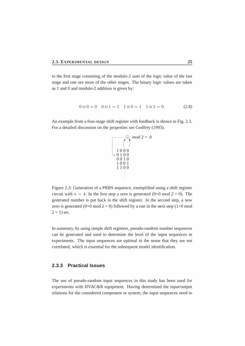
2.3. EXPERIMENTAL DESIGN 25
to the first stage consisting of the modulo-2 sum of the logic value of the laststage and one ore more of the other stages. The binary logic values are takenas 1 and 0 and modulo-2 addition is given by:
0 ] 0 = 0 0 ] 1 = 1 1 ] 0 = 1 1 ] 1 = 0. (2.8)
An example from a four-stage shift register with feedback is shown in Fig. 2.3.For a detailed discussion on the properties see Godfrey (1993).
1 0 0 00 1 0 00 0 1 01 0 0 11 1 0 0
mod 2 = 0
Figure 2.3: Generation of a PRBS sequence, exemplified using a shift registercircuit with n = 4. In the first step a zero is generated (0+0 mod 2 = 0). Thegenerated number is put back in the shift register. In the second step, a newzero is generated (0+0 mod 2 = 0) followed by a one in the next step (1+0 mod2 = 1) etc.
In summary, by using simple shift registers, pseudo-random number sequencescan be generated and used to determine the level of the input sequences inexperiments. The input sequences are optimal in the sense that they are notcorrelated, which is essential for the subsequent model identification.
2.3.3 Practical Issues
The use of pseudo-random input sequences in this study has been used forexperiments with HVAC&R equipment. Having determined the input/outputrelations for the considered component or system, the input sequences need to

26 CHAPTER 2. METHODOLOGY
be scaled to comply with the system constraints, such as the amplitude con-straints, number of controllable levels, sampling rate and time available for theexperiment. An example could be a valve opening and closing determined bythe PRBS values of 1 and 0, or e.g. a supply temperature switching between30, 40, 50 and 60◦C using a multilevel signal. Concerning the availability ofhardware and software for analysis, an empirical base for experiments of thecomponents in consumer installations has been established within IT-Energy .A photo of a test rig built for IT-Energy is shown in Fig. 2.4. In these setupsit is possible to excite the systems with different load characteristics withoutdisturbing any consumers. The use of pseudo-random input sequences is ad-equate for such practical experiments since they are easily controlled from acomputer implementation. Typically, fluid flows may be controlled accordingto the input sequences, while fluid temperatures cannot be controlled as ac-curately. The constraints concerning sampling rate and time available for theexperiments, are usually not critical.
Figure 2.4: Experimental setup at the Danish Technological Institute.The heat-ing system corresponds in capacity to 20 apartments, consisting of three watertanks, heat exchangers, valves, pumps and pipes as well as data acquisitionequipment.

2.4. PARAMETER ESTIMATION 27
2.4 Parameter estimation
This section presents the applied estimation method for models formulated interms of SDE’s. Parts of the mathematical description follows Melgaard (1994)closely.
There exist several parameter estimation methods for SDE’s. An extensivereview is given by Nielsen et al. (2000), where different estimation methods,such as the generalized method of moments, the efficient method of momentsand indirect inference, are discussed. Furthermore, Monte Carlo methods,transfer function models and non-linear filtering methods are reviewed. In(Hurn and Lindsay (1997, 1999)) a non-parametric method based on the max-imum likelihood principle and Monte Carlo techniques is used to estimate pa-rameters of SDE’s for simulated data. In Bianchi and Cleur (1996) an indirectestimation method of SDE’s is given. The problem of solving SDE’s numer-ically is treated in Kloeden et al. (1997) while more theoretical issues con-cerning parameter estimation in linear SDE’s are discussed in (Khasminskiiet al. (1999); Kim (1999)). Finally, parameter estimation in nonlinear SDE’sis discussed in Timmer (2000). For a more general discussion on SDE’s, see(Øksendal (1985); Gard (1988)).
2.4.1 Maximum Likelihood parameter estimation
In this section, the Maximum Likelihood (ML) estimation method, used in thesubsequent analysis, is discussed as applied to models formulated in terms ofSDE’s.
As discussed in section 2.2, dynamic HVAC&R models can often be formu-lated in terms of a system equation: (2.9):
dXt = f(Xt,Ut, θ, t)dt + G(Ut, θ, t)dwt, t ≥ 0 (2.9)
where discrete time measurements from the system are used to link the data to

28 CHAPTER 2. METHODOLOGY
the system using a system equation (2.10):
Yk = h(Xk,Uk, θ, tk) + ek tk ∈ {t0, t1, . . . , tN}. (2.10)
It should be noted that the state space formulation allows for a description thatdistinguishes between the uncertainty of the model formulation of the systemequation as well as the uncertainty in the measurements and the observationequation.
Assuming that the experimental dataY(t) = [Yt,Yt−1, . . . ,Y1,Y0] is a re-alization of stochastic variables and that the model parameters are normallydistributed, it is possible to construct the likelihood function. It is well-knownthat the ML estimates are found as the estimates which maximize the likelihoodfunction, see e.g. Goodwin and Payne (1977). The unconditional likelihoodfunction L(θ;Y(N)) is the joint probability of all the observations assumingthat the parameters are known:
L(θ;Y(N)) = p(Y(N)|θ). (2.11)
Applying Bayes rule to the likelihood function can be written as a product ofconditional densities:
L(θ;Y(N)) = p(Y(N)|θ)= p(YN |Y(N − 1), θ)p(Y(N − 1)|θ)
=( N∏
t=1
p(Yt|Y(t− 1), θ))p(Y0|θ).
(2.12)
The conditional likelihood function (conditioned onY0) becomes:
L(θ;Y(N)) =N∏
t=1
p(Yt|Y(t− 1), θ). (2.13)
2.4. PARAMETER ESTIMATION 29
The normal distribution is characterized by the mean and the covariance. Inorder to parameterize the conditional distributions, the conditional mean andconditional covariance are introduced as:
Yt|t−1 = E[Yt|Y(t− 1), θ] and Rt|t−1 = V[Yt|Y(t− 1), θ], (2.14)
respectively. Eq. (2.14) represents the one-step prediction and the associatedcovariance, which are calculated using a Kalman filter, discussed in Section2.4.2. The one-step prediction errors are calculated by:
εt = Yt − Yt|t−1. (2.15)
Then the conditional likelihood function (2.13) becomes:
L(θ;Y(N)) =N∏
t=1
((2π)−m/2 detR−1/2
t|t−1 exp(−12ε
′tR
−1t|t−1εt)
), (2.16)
wherem is the dimension of theY vector. By taking the logarithm of theconditional likelihood function, we obtain:
logL(θ;Y(N)) = −12
N∑t=1
(log detRt|t−1 + ε′tR
−1t|t−1εt
)+ const, (2.17)
the ML estimate ofθ is found as the value that maximizes the conditionallikelihood functionL(θ;Y(N)):
θ = arg minDM
N∑t=1
(log detRt|t−1 + ε′tR
−1t|t−1εt
). (2.18)

30 CHAPTER 2. METHODOLOGY
HereDM is the set of possible values forθ. It should be noted that the MLestimator is asymptotically normally distributed with meanθ and variance:
D = H−1, (2.19)
whereH is the Hessian given by:
{hlk} = −E[ ∂2
∂θl∂θklogL(θ;Y(N))
]. (2.20)
{hlk} denotes the element in rowl and columnk of H, andθj denotes elementj of θ.
An estimate ofD is obtained by equating the observed value with its expecta-tion and applying:
{hlk} ≈ −( ∂2
∂θl∂θklogL(θ;Y(N))
)∣∣∣θ=θ
. (2.21)
Hereby, Eq. (2.21) is used to estimate the variance of the parameter estimates.
It should also be noted that optimal experimental designs, as discussed in Sec-tion 2.3, may be constructed to minimize certain measures ofD, i.e. the op-timization criteria is to minimize the variance (uncertainty) of the parameterestimates. This requires however, that the model structure is known prior tothe experiment.
2.4.2 The Kalman filter
In the ML estimation method described in section 2.4.1, the one step predic-tions and associated covariances are needed for calculating the likelihood func-tion. In the estimation of the model parameters the Kalman filter is applied toestimate these quantities. It should be noted that the Kalman filter is derivedfor linear systems. For non-linear systems the extended Kalman filter, based onlinearizations of the system equation, is applied. Given that the system equa-tion is described by Eq. (2.9) and the observation equation by Eq. (2.10), theextended Kalman filter for the prediction equations become:

2.4. PARAMETER ESTIMATION 31
dXt|kdt
= f(Xt|k,Ut, θ, t), t ∈ [tk, tk+1[, (2.22)
dPt|kdt
= A(Xt|k,Ut, θ, t)Pt|k
+ Pt|kA′(Xt|k,Ut, θ, t)
+ G(θ, t)G′(θ, t), t ∈ [tk, tk+1[,
(2.23)
whereA is obtained by a linearization of the system equation (2.9):
A(Xt|k,Ut, θ, t) =∂f∂X
∣∣∣X=Xt|k
. (2.24)
Let C be the linearization of the observation equation (2.10):
Ck = C(Xk|k−1,Uk, θ, tk) =∂h∂X
∣∣∣X=Xk|k−1
. (2.25)
Applying the Kalman filter the updates attk are:
Kk = Pk|k−1C′k[CkPk|k−1C
′k + S(θ, tk)]−1, (2.26)
Xk|k = Xk|k−1 + Kk(Yk − h(Xk|k−1,Uk, θ, tk)), (2.27)
Pk|k = Pk|k−1 − KkCkPk|k−1. (2.28)
For a detailed reference on the applied estimation method, see Melgaard (1994).
2.4.3 Practical issues
Given that an initial model is formulated in terms of SDE’s, the model param-etersθ and the model states may be estimated by the ML method using a soft-ware package CTLSM, cf. (Madsen and Melgaard (1993); Melgaard (1994)).The package provides numerical estimates using a quasi-Newton method aswell as relevant test statistics. The software package has been used in a vari-ety of modelling applications for physical models, and also in the case studiespresented in this thesis.

32 CHAPTER 2. METHODOLOGY
2.5 Model validation
As the final step in the modelling procedure, the aspects of model validationare considered. Model validation is an important step in identifying models.It concerns the investigation and testing of the established model, and may beused to decide whether the model obtained from the identification procedurecan be accepted, and if not, how to improve it. If the identification method hasprovided the best possible model in the model set, the problem is to decide ifthe chosen model is a suitable one. This question can be approached in twoways, cf. Ljung (1982). One way is to evaluate the properties of the modeland decide whether it meets reasonable requirements. Another approach is tolook for other models or model types and make the comparison. The latterprocedure can be regarded as an a posteriori choice of model sets.
An appropriate first validation criterion is a preliminary comparison with themodel and the system. This comparison, which often is subjectively, may bedone by performing simulations with the model and verify that certain criteria,e.g. that the steady state performance, is reasonable. A good insight may beachieved by plotting dependent variables against simulated output. Visualiza-tion of the model performance will often give a clear indication if the modelcaptures the important features of the system, such as time constants, powerconstraints, steady state conditions etc. Furthermore, visualization of data candetect obvious model limitations and flaws, or reveal structures in the data thatcannot be absorbed in any other way, cf. Cleveland (1993).
2.5.1 Residual analysis
Many objective methods for validation of grey box models are closely relatedto validation techniques for black box models. For both types of model classesthe residual analysis, where residuals are defined as the deviation between themodel and observations from the system, is an important part of the modelvalidation. The purpose of residual analysis is primarily to check whether anyobtained information contradicts the assumptions upon which the models andmethods are built, cf. (Holst et al. (1992)). Furthermore, the residual analysis

2.5. MODEL VALIDATION 33
may be used to indicate how the model should be extended.
If the measurement uncertainty of the data is known, the amplitude of themodel residuals can be compared with the experimental uncertainty. If theuncertainty of the model output is not known directly, but is some function ofmeasured data, the model uncertainty can be calculated using the method ofpropagation of errors, (Coleman and Steele (1999)). Consider a model suchthat Φ = f(δ, γ, λ) and assume thatδ, γ, andλ are measured with knownuncertaintiesσ2
δ , σ2γ andσ2
λ, respectively. Then the uncertaintyσ2Φ in Φ can
be approximated by the error propagation formula assuming the measurementerrors of different variables to be uncorrelated, i.e., assuming the covarianceterms to be zero:
σ2Φ = σ2
δ (∂f
∂δ)2 + σ2
γ(∂f
∂γ)2 + σ2
λ(∂f
∂λ)2. (2.29)
Usually the sequence of model residuals,εi i = 1..N , is assumed to be nor-mally distributed with mean 0 and varianceσ2
ε , i.e. εi ∈ N(0, σ2ε ). Thus, the
value of the estimated varianceσ2ε can then be compared to Eq. (2.29).
The assumption that the model residuals are normally distributed is realisticfrom a theoretical point of view, cf. (Coleman and Steele (1999)). Importantidentification methods, such as the ML method in section 2.4, are built on thisassumption. Therefore, it is important to analyze whether or not the modelresiduals can be regarded as being normally distributed. In general, an ade-quate model should have residuals that are free of systematic patterns that themodel otherwise is failing to explain. Systematic deviations can be analyzedin multiple ways. A natural first step in the residual analysis is to graph theresiduals and check for outliers and non-constant variance. It is also helpfulto graph the residuals against input and output variables in order to investigatesystematic patterns in the residuals.

34 CHAPTER 2. METHODOLOGY
Time domain tests
There exist several statistical tests, that can be performed as a supplement tothe graphical test. These tests may be performed in both the time domain andin the frequency domain. In the time domain, the residuals may be tested usingnon-parametric methods (Haerdle (1990)), or by applying standard parametrictechniques (Box and Jenkins (1970)). The non-parametric techniques can beused for analyzing the distribution of the residuals. The distribution estimatecan be used in the grey box validation for the residual sequence and for themodel as a whole (Holst et al. (1992)).
Especially for dynamic models, the autocovariance function can be used totest the model residuals in the time domain. The autocovariance function isestimated by:
γε(k) =1N
N∑i=1
(εi − ε)(εi+k − ε), (2.30)
whereε is the estimated mean of the residual sequenceεi. The estimated cor-relation coefficient at lagk is:
ρε(k) =γε(k)γε(0)
. (2.31)
If the residualsεt of a scalar process are normally distributed, the estimatedautocorrelation function is:
ρε(k) =
{1 k = 0
0 |k| = 1, 2, ..,(2.32)
and
2.5. MODEL VALIDATION 35
ρε(k) ∈approx N(0,1N
). (2.33)
Approximative 95% limits for this distribution are±2σ = ±2/√N . Plots of
both, the estimated autocorrelations for the residuals and the confidence limits,provide a graphical way to test the hypotheses about the noise assumption, i.e.if the residuals are normally distributed.
Frequency domain test
In a similar manner, the model residuals may also be analyzed in the frequencydomain. The periodogram for the residuals for the frequenciesνi = i
N , i =0, 1, . . . , N/2, is:
I(νi) =1N
[( N∑t=1
εt cos 2πνit)2
+( N∑
t=1
εt sin 2πνit)2]. (2.34)
The periodogram is a frequency domain description of the variation of theresiduals, asI(νi) indicates how much of the variation of the residuals ispresent at the frequencyνi. The normalized cumulative periodogram becomes:
C(νj) =∑j
i=1 I(νi)∑N/2i=1 I(νi)
, (2.35)
which is a non-decreasing function, defined for the frequenciesνi. For nor-mally distributed residuals the variation is uniformly distributed over the fre-quencies, and is often referred to as white noise, due to the same spectral prop-erties for white light. The total variation forN observations isNσ2
ε , and hencethe theoretical periodogram for white noise is:
I(νi) = 2σ2ε . (2.36)

36 CHAPTER 2. METHODOLOGY
The theoretical cumulative periodogram is thus a straight line from (0,0) to(0.5, 1). If the residuals are white noise, it is expected thatC(νi) is close tothis line. Confidence intervals around the straight line can be calculated usinga Kolmogorov-Smirnov test, see (Box and Jenkins (1970)). The advantageof applying frequency domain test may be that it is possible to determine thefrequencies of dynamic patterns.
Further issues concerning residual analysis
The above-mentioned techniques for residual analysis are not always adequate.Both, the test in the autocorrelation function and frequency domain test, are lin-ear tools and may not be able to detect non-linearities. Non-linear treatmentcould be investigated non-parametricly functionals (Haerdle (1990)), that ac-counts for non-linearities, such as the mutual information coefficient Grangerand Lin (1994), or the lag dependent functions, proposed by Nielsen and Mad-sen (2001). For alternative methods for residual analysis, cf. (Wong (1997); Liand Hui (1994); Li (1998)).
2.5.2 Tests and physical interpretation of grey box models
If the residual analysis supports the model assumptions, the natural next stepis to investigate the physical characteristics of the model in more detail. Typ-ically, this includes the investigation of estimated parameter values, that thetime constants and model states agree with the physical characteristics etc.For an experienced practitioner these tests might be done intuitively based ona solid insight into the system. However, if the model at a first sight seemreasonable, more sophisticated mathematical methods can be applied to inves-tigate the system in more detail. These methods can indicate flaws that are noteasily found otherwise.
The estimated model parameters may be tested for significance using the factthat the ML method provides estimates that are approximately normally dis-tributed, cf. section 2.4. This enables test for the significance of the parameters,

2.5. MODEL VALIDATION 37
i.e. to test whether the parameters are significantly different from zero:
H0 : θj = 0 against H1 : θj 6= 0. (2.37)
The test quantity isθj
σjj, whereθj denotes thej-th parameter estimate andσ2
jj
the associated variance estimate. As the parameter estimates are asymptoti-cally normally distributed, the test value is t distributed, and then a t-test of thehypothesis can be performed. Using this test it is possible to neglect modelparameters in the model which are not significant with the data at hand.
Often initial guesses or a priori information about parameter values are avail-able which allow for a comparison if the parameter values are reasonable.Thus, the above test Eq. (2.37) may be used to test for other parameter val-ues than zero, e.g. test if an estimated physical parameter can be assumed toequal some value that corresponds to physical interpretation.
2.5.3 Cross validation and model selection
Another important test is to perform a cross validation study, i.e. to investigatethe model performance using independent data. In such a study the residualanalysis (quantitative) is not as important as a more qualitative evaluation. Thisincludes the extrapolation abilities of the model, which is usually assumedstronger for a grey box model compared to a black box model.
There exist several methods to compare sets of models. One criteria is to eval-uate if different models fulfill the criteria on residual analysis, the degree ofphysical interpretation, cross validation (Shao (1993)), and extrapolation abil-ities. Other methods are based on model selection criteria, cf. e.g. McQuarrieet al. (1997), or likelihood ratio tests Holst et al. (1992).

38 CHAPTER 2. METHODOLOGY
2.5.4 Practical issues
In general, it is advisable to combine several validation tools, since some meth-ods may be more adequate in certain situations than others. Also, the identifi-cation proceduce is an iterative process, and it is usually necessary to validatethe adequacy of model modifications. In the presented case studies in this the-sis, however, only the final validation results are presented. These validationmethods may easily be done using standard software, and in some softwarepackages, validation results are presented along with the parameter estimationresults.

Chapter 3
Overview of included papers
This section gives an overview of the included papers in the thesis. The focalpoint of each paper is the application aspect, i.e. each paper either discussesgrey box modelling techniques or models for HVAC&R components related topractical applications. Although different models and methods are presented,the main issue of each paper is the same, namely addressing the use of grey boxmodelling methods for HVAC&R components and applications. The grey boxmethods for experimental design, parameter estimation, and model validation,have been applied throughout the papers.
Paper A is an introductory paper, which presents the modelling perspectivesof the joint project IT-Energy. A short introduction to the scope of applica-tion, with emphasis on the design of simulation models for energy analysisof HVAC&R components and systems, is given. Issues concerning the devel-opment of the simulation models are discussed, e.g. on determination of themodel interface, relevant time scale and aspect of simplicity versus complex-ity. This discussion is of more or less general nature and an indirect resultof the research work developed through IT-Energy and inspired from topicsin the literature. The paper also presents more project related issues, such asexperimental setups and model validation issues as well as a discussion on theapplied modelling method. The paper is modified from its original version by
39

40 CHAPTER 3. OVERVIEW OF INCLUDED PAPERS
excluding the modelling examples. These are instead referred to as Paper C andF in the thesis. The paper is intended as a presentation of IT-Energy to otherresearchers within the field of HVAC&R and is therefore somewhat broad. Inthis thesis it serves as an introduction to and background for the subsequentpapers, which deal more specifically with detailed modelling of the HVAC&Rcomponents.
As the first paper on modelling of HVAC&R components, Paper B discussesthe aspects of experimental design related to heat exchanger modelling. Theaim of the experiment is to collect data for a succeeding modelling of the heatdynamics of the heat exchanger. The paper addresses issues relevant to thedesign of input sequences and discusses a method for generating input signals.The experimental setup is presented as well as an analysis of the experimentaldata. Finally, the data is used to validate a dynamic model of the heat dynam-ics of the heat exchanger. The main objectives of the paper are 1) to stress theimportance of and 2) to illustrate techniques for designing appropriate experi-ments for HVAC&R components. The design of input sequences is related todesign of Pseudo Random Number Signals. These signals have proven usefulin system identification and can easily be applied to other components. Also,practical aspects are discussed. These include the choice of experimental setup,sampling time, and investigation of time constants.
The modelling of the fluid dynamics in pipes is presented in Paper C. Empha-sis is put on how statistical methods can be used to build physical thresholdmodels. Threshold models may be useful in the modelling of HVAC&R com-ponents since it is a method to account for model discontinuities, e.g. change inflow characteristics or a valve closing. The method of using a smooth thresh-old function may be useful for parameter identification and for simulation pur-poses. The paper describes the experimental setup and design of input vari-ables as well as the applied threshold function. The estimation procedure isdiscussed and the results are presented. Although applied to the modelling ofthe fluid dynamics in pipes, the method may be used for other applications aswell.
A dynamic model of a radiator is presented in Paper D. The model is obtainedfrom physical reasoning and experimental data. A main issue about the model

41
is that the lumping of the radiator is done with varying section sizes dependingon the flow. The lumping technique of equal section sizes is well known frommany systems and the resulting model is obtained in terms of ODE’s. How-ever, preliminary analysis and physical interpretation suggest that there is anadvantage in using varying section sizes. Especially it is found that the varyingsection sizes are helpful for reducing the model order. The model performanceis illustrated and applications and limitations are discussed.
Paper E presents a model of a thermostatic valve with hysteresis effects. Hys-teresis is a phenomenon that appears in many physical systems and which isnot easily modelled. In this paper an adaptive model for friction compensationaccounts for the hysteresis. Using experimental data the effects from hysteresisare clearly seen and has been analyzed. The valve position is determined by asteady state expression based on physical reasoning. By formulating the modelin terms of SDE’s the unknown quantities, especially the hysteresis force, areestimated. The model performance is illustrated and further extensions of themodel are discussed.
While Papers B-E concern modelling and modelling aspects of single com-ponents, a model of a system, namely a model for the heat dynamics of abuilding, is presented in Paper F. The model is used for a building consistingof three rooms that are affected by inputs from the sun, ambient air, and radi-ators. Simple models are used to describe these external sources. The modelapproximations, and especially the simplified grey box approach, is discussedas compared to more traditional methods. The model is estimated and vali-dated using experimental data from designed experiments and both physicalinterpretation and statistical techniques are used to validate the model. In sum-mary, this model shows how simple models can be connected in order to modelmore complex system and also stresses the importance of empirical methodsin deriving such models.
Finally, Paper G presents a regression approach (Error in Variable) as a meansof identifying unbiased physical parameter estimates. The paper is differentfrom Paper A-F in the fact that the model, which is a grey box model of theCoefficient of Performance for a commercial chiller, is only used for steadystate calculations, and not in terms of SDE’s. The paper investigates the use

42 CHAPTER 3. OVERVIEW OF INCLUDED PAPERS
of the model for fault detection and diagnosis. It is illustrated that sources ofnoise, such as measurement error, may influence the physical parameter esti-mates in terms of bias and thus influence on the quality of the fault detection.The error in variable approach is applied to illustrate how the bias arising frommeasurement errors can be removed. Furthermore, the paper suggest differentmethods for correction for the measurement error bias for steady state grey boxmodels.
Chapter 4
Conclusion
The main issue in this thesis has been the application of the grey box modellingmethod to dynamic models of HVAC&R components. The application aspectsand the applied methodology have been presented in the summary report, whilethe research work consists of 7 case studies. The case studies demonstrate thetechniques and benefits in combining the deductive and inductive approach inthe modelling of typical HVAC&R components. As in the summary report,the papers focus on the grey box modelling process and distinguish betweenthe disciplines of experimental design, parameter estimation, and model esti-mation, as interrelated disciplines in building models. These methods are ofprimary interest, whereas the models are found as the best choice given thedata. In that respect, the thesis does not give a set of ’optimal’ models, butpoints out how statistical methods can be applied to handle modelling prob-lems that cannot be solved easily otherwise.
As the first step in the modelling procedure, Paper B discusses issues relevantto experimental design for subsequent dynamic modelling of HVAC&R equip-ment. The paper discusses the design of input sequences for heat exchangermodelling and the quality of the acquired data. Experimental designs have alsobeen applied in the modelling of the flow in pipes in Paper C, and in Paper Fconcerning the modelling of the heat dynamics of buildings. From the researchwork it is concluded, that there are, in general, obvious benefits in performing
43

44 CHAPTER 4. CONCLUSION
experiments with a system whenever this is possible. By proper experimentaldesign it is possible to acquire data that is informative and representative forthe system. This is helpful in the subsequent model identification comparedto non-intrusive experiments, where the variables are measured but cannot becontrolled. Even if the input variables can be controlled, there is most often aset of constraints to a given experiment that has to be accounted for. However,a well-planned experiment can ensure that data spans the modelling space andthat it is possible to identify the dynamics of interest given these experimen-tal constraints. For the experimental designs applied in this study it has beenfound that the use of Pseudo Random Number Signals (RPNS) are adequateand the signals can be constructed to meet typical experimental constraints. Inthat respect the PRNS provide input sequences that are optimal for the subse-quent parameter estimation and model validation. It can be argued that moresophisticated experimental designs could have been applied in case an a priorimodel structure was assumed. The use of PRNS included a trade off betweenvery detailed experimental plans and simple or non-intrusive measurements.It is concluded that the use of PRNS along with the well-defined experimen-tal conditions available has provided high quality data for subsequent analysis.The PRNS have desirable statistical properties and are easy to generate andcontrol in experiments. However, an interesting aspect would be to investigatethe benefits and difficulties with more sophisticated experimental designs.
The ML method for parameter estimation has been applied in the Papers B-F.The advantage of determining model parameters by statistical methods is thatthese parameter values may not easily be known or calculated otherwise. It isconcluded that the ML method is adequate for modelling of HVAC&R com-ponents because it allows for estimating both, model parameters and modelstates, in models formulated in terms of SDE’s. A key advantage of the MLmethod is that the continuous time formulation ensures that the models arephysically meaningful and that the model parameters can be interpreted di-rectly. Furthermore, the ML parameter estimation technique may provide es-timates of state variables that are non-observable and of interest in simulationstudies, e.g. the hysteresis force of the thermostatic valve in Paper E or thetemperature of the floor in the heat dynamics of buildings in Paper F. From astatistical point of view, the parameter estimates provided by the ML methodare normally distributed and this can be exploited by statistical tests for param-

45
eter significance and model reduction. Hereby, it can be statistical determinedwhich terms that are significant in a physical model. A drawback is, however,that the ML method requires knowledge in statistical modelling. Furthermore,the ML method provides estimates that are optimal to fit the data and doesnot question whether the model is adequate or not, with respect to physicalmeaning. In such cases physical insight can be used to determine whether themodel gives sound results or not. If the model assumptions for the ML methodare not valid there may also be doubts for the subsequent inference made bythe model. In such cases the method could be regarded as a prediction errormethod and the parameter estimates as values that gives the best fit in termsof predictive ability. Another aspect is that the ML method provides estimatesoptimal for one-step prediction while for many applications the real purposeis simulation. It would be possible to modify the optimization criteria to ac-count for the simulation performance of the model instead. The drawback withthis issue is, however, that the properties and assumptions of the model mayfall apart and influence on the tests for model validation. In such case a moresubjective validation criteria must be applied.
The techniques for model validation give some criteria for model verifica-tion. These techniques are well known from system identification and serveas a complement to the physical interpretation of the system. The techniquesdemonstrated in paper B-F are to some extent objective measures and relatedto residual analysis. This makes sense because it can be used to validate theprediction performance as well as the model assumptions. These techniquesdo not, however, reveal whether the model is adequate or detailed enough forother applications, for e.g. extrapolation studies, although a grey box modelshould be more reliable in extrapolation compared to a black box model. Todetermine the extrapolation abilities, the physical interpretation of the modelcan be used for further analysis, such as sensitivity analysis. A conclusionis that the techniques related to residual analysis are adequate to determinewhether the model explains the data. The physical interpretation and tests forparameter significance are also helpful in deciding whether the model is ade-quate. However, when the physical interpretation of the model is crucial, thepresented validation methods should only be used as a supplement to the modelselection process. The presented validation methods primarily reveal featuresin the data, and cannot be used as a substitute for physical insight.
46 CHAPTER 4. CONCLUSION
From a practical viewpoint the presented models have been used in the de-velopment of a simulation tool for heating systems. Although the thesis doesnot directly concern the development of the simulation tool, it is argued thatthe grey box modelling method can be used to establish adequate models forsimulation purposes compared to other modelling approaches. The term ’ade-quate’ is relative to the modelling objective. In simulation studies a low modelorder can reduce the computational effort and hereby increase the speed of thesimulations. In some cases a low model order is necessary in order to makesimulations computationally feasible. Examples of models that are computa-tionally ’fast’ are presented in Paper B, C and D. Paper D presents a dynamicmodel of a radiator where the model order is reduced due to the introductionof variable section sizes in the lumping of the radiator. This makes simulationscomputationally faster compared to a model with a large number of sections.Other modelling aspects are influencing the computational speed as well. PaperC presents a dynamic model of a pipe where the regime between the turbulentand laminar flow is modelled using a smooth threshold. This is an advantagein simulation studies because algebraic loops may be avoided (solvability), i.e.an algebraic routine that determines whether the actual flow is laminar or tur-bulent. As a third example, the heat exchanger model is evaluated in paper B.The statistical expression used for the heat transfer coefficient is both, accu-rate and computationally fast, as compared to deterministic expressions for theheat transfer coefficient. The other main characteristic is that the models are di-rectly physically interpretable. This means that practitioners not familiar withstatistical issues or modelling techniques can interpret the model parametersand model states. For simulation purposes the practitioner may experimentwith different parameter values to investigate the behavior of the componentbecause the parameters have physical meaning. For example, the behavior ofthe thermostatic valve presented in Paper E can be investigated when certaincharacteristic parameters are modified. This is beneficial e.g. in developingnew components or improving the understanding of the existing ones. Anotherexample is the chiller model evaluated in Paper G. Here the COP of the chillermay be investigated as the thermal resistance is varied.
In summary, stochastic models of HVAC&R components have been presentedwith emphasis on dynamic grey box modelling and it’s benefits for practi-cal applications. As with most modelling problems there is always room for

47
improvement. Possible improvements include performing of more sophisti-cated experiments, and investigating different model types and modelling tech-niques, e.g. residual analysis for non-linear effects. However, the overall con-clusion of the research work is, that grey box models, in terms of SDE’s, aresuitable for describing the dynamics of the considered HVAC&R components.This is due to the fact that both, the physical knowledge about the componentsis well established and that data is possible to control and acquire.

48 CHAPTER 4. CONCLUSION

Part II
INCLUDED PAPERS
II
49


51
List of papers
The case studies presented in the following have been published, presented, orsubmitted to the following journals or conferences:
Paper A: Andersen, K.K. and Poulsen, H. (1999). Building integrated heatingsystems.Building Simulation ’99, Kyoto, Japan, 1, 105–112.
Paper B: Andersen, K.K., Palsson, O.P., Madsen, H., and Knudsen, L.H. (2000).Experimental design and setup for heat exchanger modelling.Interna-tional Journal of Heat Exchangers, Accepted for publication.
Paper C: Andersen, K.K., Lundby, M., Madsen, H., and Paulsen, O. (1999). Iden-tification of continuous time smooth threshold models of physical sys-tems.Presented at the Joint Statistical Meetings, Baltimore, 1999.
Paper D: Andersen, K.K., Hansen, L.H., and Madsen, H. (2000). A model for theheat dynamics of a radiator. Submitted.
Paper E: Knop, O., Andersen, K.K., Madsen, H., Gregersen, N.H., and Paulsen,O. (2000). Modeling of a thermostatic valve with hysteresis effects. Sub-mitted.
Paper F: Andersen, K.K., Madsen, H., and Hansen, L.H. (2000). Modelling theheat dynamics of a building using stochastic differential equations.En-ergy and Buildings31 1, 13-24.
Paper G: Andersen, K.K., and Reddy, A. (2000). The error in variable (EIV) re-gression approach as a means of identifying unbiased physical parameterestimates. Submitted.

52

Paper A
BUILDING INTEGRATEDHEATING SYSTEMS
A
53


55
ABSTRACT
This paper presents the preliminary modelling perspectives of an ongoing proj-ect where a flexible simulation tool for component and system analysis of dis-trict heating consumer installations is developed. The simulation tool makesit possible to simulate district heating consumer installations containing wa-ter based central heating systems, domestic hot tap water systems, buildingsas well as load predictions of the systems. The main purpose of the projectis to improve the inter action of the system components, decrease the energyconsumption and analyze the performance of the heating system and the rela-tion between the building and the heating system, Building Integrated HeatingSystem. This is done with emphasis on increasing the system performanceof the district heating system. The paper presents the modelling approachwith main emphasis on lumped parameter modelling using statistical methods.Some prior results are discussed and illustrated through examples, includinganalysis of the heat dynamics of a building and a new approach on handlingdiscontinuities exemplified in the modelling of the transient flows pipes.
Keywords: Building Integrated Heating Systems, District Heating Systems,Lumped Parameter Modelling, Simulation studies.
1 INTRODUCTION
Since the first energy price crisis in the early seventies the energy policy inDenmark has been focused on how to reduce the consumption and the depen-dency of a single fuel. In recent years the energy demand in new buildings inDenmark has been reduced considerably due to new building regulations. Thereduced heat demand and the growing focus on the indoor climate increasesthe requirements of the performance of the heating system and the interactionbetween building and the heating system, Building Integrated Heating System.More than 60 % of the heat consumption is based on district heating (DH) dueto the national energy plans since the second energy crisis in the late seventies.Today the systems are characterized by pooled operation with combined heat
56
and power plants mainly based on incineration, coal and natural gas. The sup-pliers have made a great effort on optimizing the system performance in orderto minimize the costs; during the last fifteen years the optimization processhas focused on the production plants and the distribution systems. Integrationof the consumer installations in the process started around five years ago, asthe natural last step in optimizing the overall efficiency. The design and op-eration of the consumer installations are improved with respect to the systemperformance, i.e. the installations must operate at a low temperature level witha high cooling and few peaks. The manufacturers of the components are veryimportant in this process and the product development has changed from fo-cusing on the component (sub optimization) to focusing on the inter action ofthe components (system optimization). Developing new products or improv-ing existing is traditionally a complex and expensive task including numeroustests in the lab followed by final tests of a prototype in situ. Today a largepart of these tests can be replaced by computer simulation studies. The use ofdynamic models in computer simulation studies has proven to be a perceptiveand practical method to analyze the performance and the control strategies inheating systems. Thence, the dynamics of the heating system can be analyzedsecond by second with varying heat supply from persons, machines and thesun in order to minimize the heat demand in the buildings and optimize thethermal comfort. However, the prospects from applying simulation studies indevelopment of system components depend strongly on the accuracy and flex-ibility of the models used for the simulation. The paper presents the modellingapproach and the idea behind a project concerning the development of a modellibrary for simulation purposes.
2 THE MODELLING OBJECTIVE
The project is a joint project with collaborators from some of the largest man-ufacturers of DH components in Denmark and public research institutes. Themodelling objective of the project is to establish a model library of the com-ponents in typical DH systems, sketched in Fig. 1, as a foundation for systemanalysis, simulation studies and product development. An essential aspect ofthe project, is, that the modelling of system components is continuously val-

57
idated on experimental data to ensure accuracy and reliability in analysis andsimulation studies. For this reasons an experimental setup are used as an em-pirical base for model validation.
In order to analyze the influence from the heating system on the indoor climatethe models are divided into two categories, namely:
(i) Models of system components.
(ii) Models of the total system.
The models of system components are gathered in the model library and maybe used for analyzing purposes and simulation studies. The user of the modellibrary can select components from a graphical user interface (GUI) environ-ment. Specific arrangements or setups are created using a drag-and-drop tech-nique of the components into a worksheet, where the components are con-nected into a desired setup. The model library includes models of:
• Plate heat exchangers.
• Radiators.
• Thermostatic and pressure relief valves.
• Pipes and fittings.
• Pumps.
• Thermal zones and buildings.
By descending order, each class of the components cf. above, contain differ-ent models of each component. The models may vary in complexity, controlstrategies and user interface. Furthermore, each component may be adjusted toa specific product, i.e. physical properties such as heat capacities, resistances,sizes etc. may be controlled by the user.

58
Fig. 1: Sketch of a typical DH system. The combined heat and power plantsupplies the consumer via heat exchangers with hot water (solid line) for heat-ing and domestic water. After consumption, the cooled water (dotted line)returns to the power plant.
The model interface
As sketched in Fig. 1 the total DH system besides the dynamics of the powerplant is considered. The system is affected by climate variables as well as theload from the power plant, interaction between components, human activityetc. In order to achieve a well-defined user interface, only the models of thetotal system and entire rooms and buildings may be affected directly by theclimate variables, such as the outdoor temperature, solar radiation etc. Systemcomponents, such as radiators and valves, are only indirectly affected by theclimate variables, i.e. via the building in which they are placed. The interfaceof the system components are indoor temperatures, supply- and return watertemperatures as well as flow and pressure drop in pipes.
The models of system components used in the simulation tool are mainlylumped parameter models. There are several arguments for preferring and us-ing lumped parameter models for system components compared to black boxmodels and models in terms of partial differential equations. Firstly, lumpedparameter models based on the laws of nature are directly physically inter-pretable, a key issue where the black box models fail. Secondly, lumped pa-rameter models in terms of ordinary differential equations are far simpler toestablish and for simulation purposes compared to distributed parameter mod-

59
els, i.e. models in terms of partial differential equations. The lumped parametermodels may be used for ’stand alone’ simulation studies or together with othermodels of components in simulation studies of component interactions. Themodels of a total system may in principle be a system of lumped parametermodels, corresponding to a setup of lumped parameters models of the com-ponents in the system. However, for large scale simulations, this may not benecessary or even to complex a task. When only the relation between the in-put and the output signals of the system is of interest, the transfer functionrepresentation is regarded as a sufficient description of the system. The userinterface is still physically interpretable, e.g. flow rates, supply temperaturesand pressure drops, whereas the transfer function from input to output is notphysically interpretable.
3 THE EXPERIMENTAL SETUP
In order to get an empirical base for the dynamical models of the componentsin the consumer installation the input-output relationship and dynamical char-acteristics of each component as well as the interaction between the systemcomponents are investigated in an experimental setup. This section presents adesigned test rig for detailed testing of DH system components.
The experimental setup, a 100 kW test rig, corresponding to 20-30 apartments,represents a typically consumer installation in Western European countries.The heating system is separated from the DH system by a heat exchanger. Theradiator system is divided into three individually zones, where hot water tanksemulate the dynamics of each zone. The load in the domestic hot water systemis emulated by predictions, i.e. tap programs from a computer. The domestichot water is produced instantaneous in a heat exchanger. In the main setup ofthe heating system only the load from the radiator system is of importance,not the performance of the individual radiator. Therefore, the empirical dataof the radiator is assembled in a separate set up, where thermo-vision is usedto verify the heat transfer from the radiator. The heat exchangers, radiatorsand hot water tanks are connected through pipes and fittings where pumps andvalves controlled by a computer may generate pre-specified operating condi-

60
tions. Furthermore the setup has the possibility for hardware-in-the-loop sim-ulations, where new products, such as controllers and pumps, can be analyzed.The test rig are used for a variety of experiments and applications, such asmodel analysis and hardware-in-the-loop experiments, diagnosis and failuredetection as well as data acquisition for modelling and simulation purposes.
4 THE MODELLING METHOD
The modelling of system components are based on the physical characteris-tics of the components and empirical data from the experimental setup. Thissection presents briefly the modelling method for establishing physically inter-pretable lumped parameter models of system components using state-of-the-artmodelling techniques. The emphasis is made on the total modelling processand the modelling method is illustrated through examples.
4.1 The grey box modelling method
The lumped parameter models of the system components included in the modellibrary are designed wrt. two main criteria:
∗ Accurate static and dynamic simulation performance.
∗ The model interface.
To comply with the design criteria, (i) and (ii), a novel modelling method, thegrey box modelling method, see Melgaard (1994), is applied. The method hasproven adequate for modelling components in DH systems, see e.g. Palsson(1993); Sejling (1993); Hansen (1997). The total modelling process may bedescribed by a flowchart, consisting of the three stages, sketched in Fig. 2.The modelling process is characterized by that both physically insight, statis-tical methods and experimental data are used to identify the model structure,estimate model parameters, estimate the model uncertainty and validate themodel.
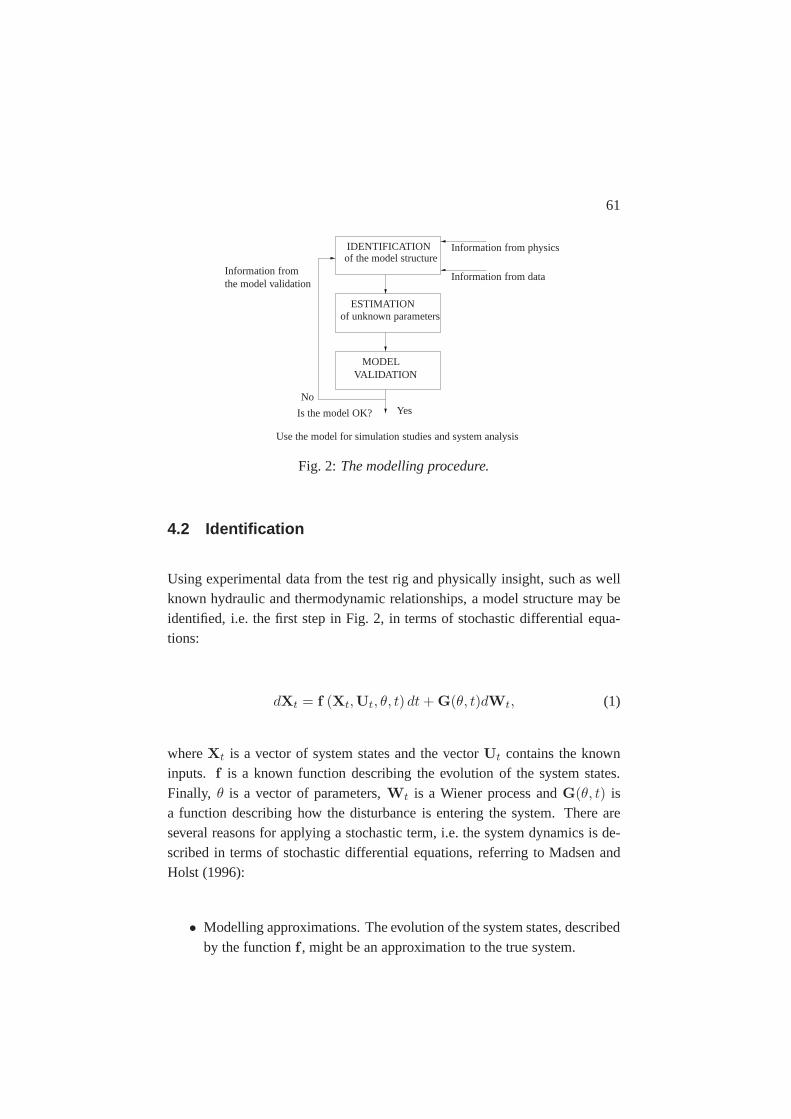
61
IDENTIFICATIONof the model structure
NoYes
ESTIMATIONof unknown parameters
Use the model for simulation studies and system analysis
Is the model OK?
MODELVALIDATION
Information from physics
Information from dataInformation fromthe model validation
Fig. 2: The modelling procedure.
4.2 Identification
Using experimental data from the test rig and physically insight, such as wellknown hydraulic and thermodynamic relationships, a model structure may beidentified, i.e. the first step in Fig. 2, in terms of stochastic differential equa-tions:
dXt = f (Xt,Ut, θ, t) dt+ G(θ, t)dWt, (1)
whereXt is a vector of system states and the vectorUt contains the knowninputs. f is a known function describing the evolution of the system states.Finally, θ is a vector of parameters,Wt is a Wiener process andG(θ, t) isa function describing how the disturbance is entering the system. There areseveral reasons for applying a stochastic term, i.e. the system dynamics is de-scribed in terms of stochastic differential equations, referring to Madsen andHolst (1996):
• Modelling approximations. The evolution of the system states, describedby the functionf , might be an approximation to the true system.

62
• Unrecognized and unmodelled inputs may affect the evolution of thestates.
• Measurements of the input are noise-corrupted.
Thus, a model formulation in terms of stochastic differential equations ac-counts for that the functionf only is an approximation to the true evolutionof the system states. The continuous time model formulation based on laws ofnature ensures that the the model structure is directly physical interpretable.
4.3 Parameter estimation
Having measured some of the state variables, a state space representation canbe formulated
dXt = f (Xt,Ut, θ, t) dt+ G(θ, t)dWt, (2)
Yt = h (Xt,Ut, θ, t) + et, (3)
whereYt is a vector of the actually observed state variables. Eq. (2) is acontinuous-time system equation and Eq. (3) is the discrete time observationequation. The functionh describes the relationship between the state variablesXt and the measurementsYt. et is a vector describing the measurement noisewhich is assumed to be Gaussian distributed. The parameter vectorθ containsthe equivalent thermal and hydraulic components, i.e. capacitances, resistancesetc., and is estimated by a Maximum Likelihood (ML) method. Descriptionsof the ML method can be found in Ref. Melgaard (1994).
4.4 Model validation
The last stage in the modelling process concerns the model validation. Themodels are validated using both experimental data, statistical validation tech-
63
niques and physically interpretation. The latter by comparing the model pa-rameters, such as time constants and the estimated model parameters,θ, withthe equivalent physical characteristics of the system. As a supplement to thephysically interpretation of the model, statistical methods are applied. By us-ing stochastic independent data from the test rig and statistical methods, themodels are cross validated. Hereby, it is possible to determine the goodness-of-fit using statistical criteria such as residual analysis, test for model order,test for parameter significance etc. If the model validation indicates an inade-quate model performance, information from the model validation can indicatehow to improve the model structure, as indicated in Fig. 2.
5 MODELLING EXAMPLES
This section gives two examples of models included in the model library. Thefirst example illustrates the modelling of a total system, namely an approach onthe modelling of the heat dynamics of a building. It is argued how to extend theanalysis by applying dynamic models of system components such as radiatorsand thus achieve a more detailed model. The second example concerns theanalysis and modelling of a single component, namely the transient flow ratesin pipes. Emphasis is made on a method for handling model discontinuities.
∗ The modeling examples are left out and given in:Paper F:Modelling the heat dynamics of a building using stochastic differentialequationsandPaper C:Identification of continuous time smooth threshold models of physicalsystems.
6 CONCLUSION
The paper described the aim and preliminary analysis of an ongoing project.The aim of the project is to develop a simulation tool for simulation purposes

64
of DH systems in order to improve on the interaction between system compo-nents and between the building and the heating system. The modelling methodhas been described with emphasis on the identification process of lumped pa-rameter models where statistical methods are applied in estimation and modelvalidation. The simulation tool may be used for simulation of system compo-nents or for simulation of total systems. The latter may be done by creating aspecific setup using models of system components. The modelling method wasillustrated through two examples. The first example described the modellingof the heat dynamics in buildings. The model parameterization was found ade-quate using statistical methods. It was discussed how a simulation study couldbe more detailed by applying dynamic models of system components. Thesecond example illustrated a new method for handling system discontinuities.The method was illustrated in the modelling of single component, namely amodel of the transient flow in pipes.

Paper B
EXPERIMENTAL DESIGNAND SETUP FOR HEAT
EXCHANGER MODELLING
B
65


67
ABSTRACT
This paper deals with the design of input variables for an experimental setupof a counter-flow heat exchanger arrangement. The aim of the experiment isto collect data for a succeeding modeling of the heat dynamics of the heatexchanger. The paper discuss issues relevant to the design of input sequencesand a method for generating multi-level random signals is introduced. Thesignals are designed to excite the non-linear dynamics of the system properlyand to avoid correlation between input variables. The quality and statisticalproperties of the data from the experiment are discussed and the simulationperformance of a dynamic model is illustrated.
Keywords: Counter-flow heat exchanger; Experimental Design, Pseudo Ran-dom Number Signals, Non-linear system.
Nomenclature
b = slopeC = constantC
′= constant
f = function describing the system dynamicsh = functionh = heat transfer coefficientk = thermal conductivityk
′= time lag
K′
= constantm = constantn = order of the PRBS sequencen∗ = number of compartmentsNu = Nusselt numberPr = Prandtl numberq−1 = back shift operatorRe = Reynolds number

68
T = temperatureU = input vectorX = state vectorY = output vector
Greek symbols
θ = parameter vectorλ = base time interval in the PRBS sequenceµ = dynamic viscosityτ = time constantφ = filter parameter∆t = sampling interval
Subscripts and superscripts
c = cold sideh = hot sidein = inputk = discrete time indexout = outputt = continuous time indexx = exponenty = exponent

69
1 INTRODUCTION
The use of statistical methods is well recognized in identification of modelsfor HVAC components. Less attention has been given to the aspect of exper-imental design, an important step in establishing reliable models. Basically,experimental design deals with the methods and techniques used in the designand analysis of experiments. It is the connection between the experiment andthe model that the experimenter can develop from the results of the experiment(Montgomery (1991)).
In order to identify empirical relationships for models of HVAC componentsthe quality and statistical properties of data used for model identification andfor model validation should be adequate. It is important that significant vari-ables are measured at a suitable sampling rate, that strong correlation betweenvariables is avoided, that the data is accurate and span the modeling space well,that data are persistently exciting etc. A well-planned experimental design canhelp achieving this goal. For identification of dynamics systems optimal inputsequences may be obtained by using Pseudo Random Number Signal (PRNS)sequences. The generation of PRNS sequences is discussed intensively in theliterature for applications in engineering, see e.g. Godfrey (1980); Yarmolikand Demidenko (1988); Nowak and Veen (1993); Godfrey (1993). However,only a few studies report the use of such signals for experiments concerningHVAC equipment. Binary multi-frequency signals have been applied in identi-fication of a large water-heated cross-flow heat exchanger in Franck and Rake(1985). Binary signals have also been applied for linear models of the heat dy-namics of buildings, see Madsen and Holst (1995); Hansen (1997); Andersenet al. (2000).
This paper deals with the analysis of an experimental setup and input designof a heat exchanger arrangement. Important issues concerning the quality andstatistical properties of the experimental data are discussed. In Section 2 the ex-perimental setup is described. The experimental design is discussed in Section3. Emphasis is put on the generation of PRNS sequences that are informativeand not significantly cross-correlated. Since the heat transfer coefficient is anon-linear function of both mass flows and temperatures a method for genera-

70
tion of input sequences for non-linear systems is proposed. The experimentaldata is presented in Section 4. The statistical properties of the data are dis-cussed and the simulation performance of a heat exchanger model is illustratedusing the experimental data. Finally a conclusion with discussion is given.
2 THE EXPERIMENTAL SETUP
The considered counter-flow plate heat exchanger has the nominal power ca-pacity of 105 kW and the convector fluid is water on both sides. The dimen-sions are 1174(h)∗ 368(w)∗ 458(l) mm. In the standard setup it consists of31 plates, 0.6 mm stainless steel. The total active area is 4.93 m2, the volumeis 8.6 l and the total mass of the heat exchanger material is 180 kg. The heatexchanger is characterized as a counter flow type even though a few platespassages actually have parallel flow on each side. Furthermore, adding or re-moving plates can vary the capacity of the heat exchanger. The experimentalsetup is sketched in Fig. 1. The experimental setup is divided into a hot anda cold side, and the inlet and outlet temperatures as well as the mass flow aremeasured on each side. For subsequent modeling purposes the variables arecharacterized as follows:
• Controllable Inputs: The two inlet temperatures and the two mass flows.
• Measured Outputs: The two outlet temperatures.
During experiments it is possible to switch the flow within 4 levels and thetemperature within 2 levels at each side, respectively. On both the hot and thecold side of the setup two tanks of water with the desired supply temperaturesare acting as buffers in order to keep the supply temperatures constant. Byusing a PID-controller and several valves and a by-pass loop (not sketched)the flow can be controlled at 4 different levels at each side. The temperaturesensors,1.0 mm, type K (Ametek), are placed close to the inlet and outletof the heat exchanger. The accuracy of the sensors is estimated to be withinthe±0.5◦C range of the actual temperature. The mass flow on both sides ofthe experimental setup is calculated indirectly by measuring the pressure drop

71
80◦C 70◦C 40◦C 30◦C
Tc,in
Th,out Th,in
Tc,out
mh
mc
Fig. 1: Sketch of the heat experimental setup.T denotes temperature andmdenotes mass flow. The indexh is used for the hot side andc is used for thecold side.
while the water passes through a blender. The sensors, type Endress Hauser,Deltabar PMD 130, are estimated to measure the actual flow within an accu-racy of±0.1% in the considered range. The motivation for using a blenderinstead of a traditional flow sensor is, that time constant of the blender is muchsmaller than a typical flow sensor. However, a traditional flow sensor, Danfoss,is used in the experimental setup, to verify the measurements by the blenders.A converter, 6BP16-2 Backplane (National Instruments) and data acquisitionsystem, Labview, are used to control the input variables and to collect the de-sired measurements during the experiment.
3 DESIGN OF INPUT VARIABLES
This section presents the design of input variables for the heat exchanger setup.Emphasis is put on how to combine physical knowledge and statistical methodsin order to design the input variables.

72
The physical structure and interpretation of HVAC models and systems is im-portant for analysis and applications, e.g. for system design, simulation studies,design of control strategies, fault detection and diagnosis etc., see e.g. (Jons-son et al. (1992); Jonsson and Palsson (1992, 1994); Bourdouxhe et al. (1998);Weyer et al. (2000)) for heat exchanger applications. Furthermore, it is attrac-tive to combine empirical data and physical knowledge in order to identify andvalidate these models (Ljung and Glad (1994)). In the design of experimentsthe physical knowledge of the system can guide the selection of appropriateinput levels, sampling rate and in determining what variables that should bemeasured etc. In the experimental design, statistical methods are useful as asupplement to the physical interpretation of the system. Statistical methodsare useful in constructing input sequences that maximize the information inempirical data and in ensuring that the experiment is randomized properly andthat the measurements are not significantly correlated.
In this study the input variables may be controlled. Hence, the aim of the ex-perimental design is to generate input sequences that both excite the dynamicsof the heat exchanger properly and span the modeling space well. The rangeand level of the input variables are determined from physical interpretation,i.e. corresponding to the maximum range of the typical operating conditions aswell as levels in between. The switching of the signals is determined by PseudoRandom Number Signal (PRNS) sequences. Using PRNS sequences, as inputsignals in experiments with dynamic systems, is attractive because of the nicestatistical properties for system identification. The PRNS have properties simi-lar to white noise, i.e. a PRNS signal may be constructed and controlled so thatit is not significantly correlated to other measured variables. This importantproperty makes it easier to separate the impact from different variables on thesystem and thus establish reliable empirical relationships (Chatterjee (1991)).
The generation and statistical properties of PRNS sequences is investigatedintensively in the literature, see e.g. Godfrey (1980, 1993) or Yarmolik andDemidenko (1988). The PRNS sequences are absolute stable and determinedby the algorithm for pseudo random number generation. The sequences are de-terministic and may be repeated from any desired implementation segment sothere is no need for storage capacity. In this paper we distinguish between twotypes of PRNS signals, the Pseudo Random Binary Signal (PRBS) sequences

73
and the Pseudo Random Multilevel Signal (PRMS) sequences. The PRBS hastwo levels and the PRMS has three or more levels. A possible method to gen-erate a PRBS sequence is to use a shift register, sketched in Fig. 2. The PRBSis constructed by selecting the shortest (λ) and the longest time interval (nλ)where the signal is constant. The signal may switch from one level to the otherat certain intervals of time,t = 0, λ, 2λ, .., nλ. The shift register determinesthe switching of the signal. The signal is periodic with the periodλ(2n − 1).The shift register has feedback to the first stage, and consists of the modulo-2sum of the logic level of the last two of the other stages. See Godfrey (1993) forothern and a detailed discussion on generation of PRBS sequences. However,concerning heat exchanger modeling, the heat transfer coefficient is known tobe a non-linear function dependent upon both mass flows and temperatures.Due to the limitation of the PRBS in only consisting of two levels, PRBS maynot sufficiently excite nonlinear systems, see Nowak and Veen (1993). For non-linear system identification, PRMS sequences may be more adequate, since ahigher number of levels may be selected. We propose a method to construct thePRMS sequence. The method is simple and straightforward and quite similarto the above method for generation of PRBS sequences. Using two differentshift registers, two independent PRBS sequences are generated. The four pos-sible combinations of the two PRBS signals determine the four-stage PRMSsequence, i.e.0 ] 0 = 1, 0 ] 1 = 2, 1 ] 0 = 3 and1 ] 1 = 4.
1 0 0 00 1 0 00 0 1 01 0 0 11 1 0 0
mod 2 = 0
Fig. 2: Generation of a PRBS sequence, exemplified using a shift register cir-cuit with n = 4. In the first step a zero is generated (0+0 mod 2 = 0). Thegenerated number is put back in the shift register. In the second step a newzero is generated (0+0 mod 2 = 0) followed by a one in the next step (1+0 mod2 = 1) etc.

74
Since the mass flows could be controlled within 4 levels and the temperatureseach within 2 levels the temperature signal has been determined by PRBS se-quences and the mass flow by a PRMS sequences. The selected input levels arelisted in Tab. 1. Based on steady state calculations provided by the manufac-turer, the time constants,τ , were assumed to be in the interval 4-25 seconds.These time constants are listed in Tab. 2. The calculated time constants indi-cate that the sampling time should be selected not larger than 2 seconds sinceit would not possible to estimate the fast dynamics using a lower sampling rate(Ljung and Glad (1994)). Due to the uncertainty of the estimate of the timeconstant, a sampling time of 1 second is found appropriate. The time con-stant of the sensors is found to be much smaller[0.15 − 0.25] s and assumednot to influence on the accuracy of the measurements. The shift registers andtime intervals, used for generation of the PRBS sequences controlling the inlettemperatures, are listed in Tab. 3. The PRMS sequences controlling the massflows are listed in Tab. 4. The time intervals,λi, are selected with respect to thecalculated time constants, i.e. the smallest time interval is larger than expectedtime constants.
4 THE EXPRIMENTAL DATA
Several different PRNS sequences were applied as input variables to the exper-imental to make sure that both fast and slow excitations could be identified andsimulated by a dynamic model. Each time series had a sampling frequency of1 Hz and the length of an experimental run was 3500 s.
Table 1: The input level of the mass flows and inlet temperatures.Level Th,in [◦C] mh [kg/s] Tc,in [◦C] mc [kg/s]
1 70 0.31 30 0.322 80 0.37 40 0.393 - 0.50 - 0.524 - 0.71 - 0.77

75
Table 2: Estimated time constants.Step (from→ to) τ (Th,out) τ (Tc,out) Units
mh 0.72→ 0.36 (kg/s) 9.5 13.8 s
mc 0.84→ 0.42 (kg/s) 25.0 9.9 s
Th,in 80→ 70 (◦C) - 4.0 s
Tc,in 40→ 30 (◦C) 5.0 - s
Table 3: PRBS sequence controlling the inlet temperatures.Input Time interval[s] Shift Register
Th λ = 27 [0101001010110]Tc λ = 41 [100110]
A time series from an experimental run is shown in Fig. 3. It should be stressedthat the results presented in the following are representative for the other ex-periments as well. In general, the input variables are fairly close to the deter-ministic PRNS sequences. More precisely, the mass flows are very accuratewhile the inlet temperatures deviate slightly wrt. the input design. For the timeseries in Fig. 3 the estimated correlation coefficients between the flow andtemperature signals are listed in Tab. 5. It is seen that none of the signals arestrongly correlated with each other. The data are not considered noisy and thetime series contain non or only very few outliers. In Fig. 4 a scatter plot ofthe outlet temperature against the inlet temperature and the mass flow on the
Table 4: The two PRMS sequence controlling the mass flows. The four stagePRMS sequence is determined by the four possible combinations of PRBS1and PRBS2 and by PRBS3 and PRBS4, respectively.
Input Time interval[s] Shift Register
mh λ1 = 9 PRBS1:[0101001]λ2 = 17 PRBS2:[11000101011]
mc λ1 = 5 PRBS3:[0101001]λ2 = 12 PRBS4:[011001010]

76
Table 5: Estimated correlation coefficients between input variables.ρ(mh, mc) ρ(mh, Th) ρ(mh, Tc) ρ(mc, Th) ρ(mc, Tc) ρ(Th, Tc)
-0.05 0.08 0.32 -0.23 0.02 -0.06
hot side is shown. It is seen that the data spans well and that the data are notstrongly correlated. The same holds for the cold side (not plotted) and for othercombinations of input and output variables.
The range and variations of the data ensures that the dynamics of the consid-ered heat exchanger may be validated for a wide range of operating condi-tions. A dynamic model, reported in Jonsson et al. (1992); Jonsson and Pals-son (1992, 1994) to perform well for a small counter-flow heat exchanger hasbeen applied. The model is a lumped parameter model where both physical
Supply temperatures (◦C)
time (sec.)300015000
80
60
40
Flow (kg/h)
time (sec.)300015000
3000
1000
Fig. 3: Measured data: cold side (-.-) dotted line, hot side (–) solid line.

77
knowledge and statistical methods have been used in establishing an adequatemodel structure. Referring to Palsson (1993) it is assumed that the heat trans-fer to the surroundings is negligible and that there is no heat conduction in thefluids. The distributed character of the heat transfer can be approximated byintroducing compartments in the system (lumping). As sketched in Fig. 5, theheat exchanger is divided into compartments.mh(t) andmc(t) are the massflows on the hot and cold side, respectively. Similarly,Th,in(t), Th,out(t) andTc,in(t), Tc,out(t) are the inlet and outlet temperatures on each side.Th,i(t),Tc,i(t) are temperatures in each compartment,Tm,i(t) are the temperature ofthe intermediate metal layer compartments.
The differential equations which describes the heat dynamics of the heat ex-changer are formed by considering the energy balance equations Eq. (1-2):
d(Heat stored)dt
=∑
Power in−∑
Power out, (1)
⇒ CidTi
dt=∑
Φin −∑
Φout. (2)
Mass flowInlet temperature
50
40
302500
20001500
8070
60
Input signals vs. outlet temperature
Fig. 4: Distribution of the outlet temperature as a function of the inlet temper-ature and the mass flow (hot side).

78
Th,1(t) Th,n(t)
Tc,1(t) Tc,2(t) Tc,n(t)
Th,2(t)Th,in(t)
Tc,out(t)
Th,out(t)
Tc,in(t)
mh(t)
mc(t)
Tm,1(t) Tm,2(t) Tm,n(t)
Fig. 5: The compartmental counter flow heat exchanger model.
Dividing the heat exchanger inton equal compartments, implies for the com-partment of numberi, the following differential equations:
Mh
nchdTh,i(t)dt
= mh(t)ch[Th,i−1(t) − Th,i(t)] − Ah
nU∆Ti(t), (3)
Mc
nccdTc,i(t)dt
= mc(t)cc[Tc,i−1(t) − Tc,i(t)] +Ac
nU∆Ti(t). (4)
U is the overall coefficient for the heat transfer from one flow to the other.Here it is written as an independent parameter though it is actually a func-tion of mass flows and temperatures.∆Ti(t) is the driving force for the heattransfer representing the temperature difference between each pair of hot andcold compartments. The indexesh andc denotes the hot and cold fluid,Mc
denotes the heat capacity on each side andA the surface area of each com-partment. Dividing the heat exchanger inton compartments yields a2n ordermodel. In Eq. (3-4) the heat capacity of the metal between the liquids are ne-glected. However, the extension of including the heat capacity of the metalis straight forward, see Sejling (1993). The driving force for the heat transferrepresented by∆Ti are modeled as a weighted average of the temperatures oneach side:

79
∆Ti(t) =12[Th,i−1(t) − Th,i(t)] − 1
2[Tc,i−1(t) − Tc,i(t)]. (5)
(6)
It is well known, that the heat transfer between the fluid and the intermediatemetal is a non-linear function of both temperature and mass flow. In Jonssonand Palsson (1992, 1994) the heat transfer coefficient,h(T, m), are modeledby physical interpretation of empirical relations and statistical methods, bysimplifying (applying) the empirical relation:
Nu = CPrxRey, (7)
and inserting expressions for Nu, Pr and Re, it is shown in e.g. Jonsson andPalsson (1994) that the heat transfer can be give by:
h(T, m) = K µ(T )(x−y)k(T )(1−x)︸ ︷︷ ︸i
my︸︷︷︸ii
, (8)
whereµ(T ) is the dynamic viscosity andk(T ) is the thermal conductivityboth with dependency of the temperature, wherem is the mass flow, K is aconstant andy andx are exponents depending on the type of flow. In Eq. (8)(i) is temperature dependent and (ii) mass dependent. In Jonsson and Palsson(1994) the approximations Eq. (9) and (10) are found appropriate:
h(T, m) =K′(1 + bT )my, (9)
h(m) =C′my, (10)
whereC′
andK′
are constants andb is a slope. In Eq. (9) the heat transfer isboth mass flow and temperature dependent, but in Eq. (10) is only mass flowdependent. Finally, neglecting the resistance of the metal between the massflows, the heat transfer coefficientU can be formulated as:

80
1U
=1hh
+1hc. (11)
The heat transfer coefficient (11) may now be included in the models of the heatexchanger. In summary, the lumped model describes the outlet temperaturesas a function of the inlet temperatures and the mass flows.
By lumping the model into 3 sections at each side the model consists of 6differential equations. The model has been applied to the experimental data.Different time series have been used for parameter estimation and others formodel validation in order to validate the simulation performance of the model.A cross validation of the model using an is plotted in Fig. 6. It is seen that themodel is able to simulate the outlet temperatures with a very high accuracy.
Cross validation: return temperatures hot side (◦C)
time (sec.)200010000
60
40
Cross validation: return temperatures cold side (◦C)
time (sec.)200010000
80
60
Fig. 6: Measured data (-.-) dotted line, Simulated data (–) solid line.

81
5 CONCLUSION
An experimental setup and the design of input variables for a counter-flow heatexchanger arrangement has been presented. The aim of the experiment was tocollect data for the succeeding modeling of the dynamics of the heat exchanger.The heat exchanger was described and the construction of the experimentalsetup was discussed. Physical interpretation and statistical methods were usedto plan the experiment and to design the input sequences for the heat exchangersetup.
It was argued that in order to identify empirical relationships for models ofHVAC components the quality and statistical properties of data used for modelidentification and for model validation should be adequate. To achieve this goalPRNS sequences were applied to generate input sequences and a new methodfor generating such sequences was described. These signals were applied andthe experimental data were presented. The quality of the data was analyzedand it was argued that by applying the PRNS sequences
(i) The range and distribution of the data ensures that the model is valid fora wide range of operating conditions.
(ii) The input signals are not strongly correlated it is possible to identifyand estimate the impact from both mass flows and temperatures on thedynamics of the heat exchanger.
The generation of PRNS sequences is straight forward and has proven usefulin experiments of dynamic systems. Furthermore, the generation of PRMS se-quences may be extended to have more levels than applied in this study. Forsuccessful experiments it is required that the signals can be controlled at thedesired levels. As the number of levels increases so do the need for longerand more complex experiments in order to obtain data with adequate statisticalproperties. Thus, the price for good quality data may be a more complex ex-perimental setup. However, even simple experimental design may as discussedis this study can greatly improve the quality of data and make a subsequentmodel identification easier.

82

Paper C
IDENTIFICATION OFCONTINUOUS TIME
SMOOTH THRESHOLDMODELS OF PHYSICAL
SYSTEMS C
83

85
ABSTRACT
This paper presents a technique for identifying accurate and physically inter-pretable threshold models of physical systems by the means of physical knowl-edge and statistical methods. The modeling approach is illustrated by consid-ering typical components in a water based central heating system. The modelformulation is based on the laws of nature and statistical analysis of exper-imental data. It is shown that in many cases the dynamic characteristics ofsuch a physical system depend strongly upon the state of the system, e.g. lami-nar or turbulent flow in a pipe, and it may be difficult to obtain models that arevalid for different excitation of the input variables. A solution to this problemis suggested by introducing smooth threshold models. The models are formu-lated in continuous time by lumping the system and using stochastic differentialequations. The continuous time formulation ensures that the model is directlyphysical interpretable. A Maximum Likelihood method is used to estimate themodel parameters and the model states. Statistical methods are applied toverify that the model provides a reasonable description of the system.
Keywords: Smooth threshold models, Lumped parameter models, Stochasticdifferential equations, Maximum Likelihood method.
1 INTRODUCTION
Many physical systems are distributed systems for which the dynamics in prin-ciple may be described by physical laws and thus by partial differential equa-tions (PDE). In many applications a model formulation in terms of PDE’s isdifficult to obtain since the system is to complex and may not be known com-pletely. Under such conditions a black box model (Box and Jenkins (1970))may be appropriate, even if no prior information about the process is at hand.However, in cases where some prior knowledge about the process is present, itmay be desirable to incorporate this physical knowledge into the model struc-ture. This modeling approach, where physical knowledge is accounted forand used together with the information from data is referred to as the grey

86
box modeling approach, see e.g. Tulleken (1992); Melgaard (1994); Ljung andGlad (1994).
Different modeling approaches may be applied to the same problem or phys-ical system. One example is in the modeling of Heating, Ventilation and AirConditioning (HVAC) components, such as heat exchangers and air condition-ers, where different modeling methods can be applied, see Bourdouxhe et al.(1998). However, when analyzing HVAC components, e.g. in the design ofcontrol strategies or in the developing of new products it is often desirableto incorporate physical knowledge at hand such as the laws of heat and masstransfer, or relevant physical parameters such as heat capacities and resistances.In such situations the grey box approach can be a powerful tool. The dynamicalcharacteristics of a given system may be described approximately by lumpingthe partial differential equations, i.e. obtain a model formulation in terms ofordinary differential equations (ODE). For more complex systems the ODE’smay be obtained by considering mass and heat balances. By using experi-mental data and including stochastic terms, the model can be formulated as asystem of stochastic differential equations. An advantage using this approachis that it is directly physical interpretable. Furthermore, the use of statisticalmethods permits a description of model uncertainties and provides a very use-ful tool in the model validation, i.e. to determine whether or not the modelstructure is reasonable.
However, for some HVAC components the dynamical characteristics of thesystem depend strongly upon the state of the system. Examples of such modeldiscontinuities are valves shutting down, phase transition in heat exchangersand the transition from laminar to turbulent flow in a pipe. Therefore it maybe difficult to obtain a total model which is valid for very different excitationof input variables by lumped parameter models. A commonly used approachis to restrict the model wrt. the input signals, i.e. the model is only valid forcertain ranges of the input variables, e.g. a pipe model which is only valid forturbulent flow.
In this paper an approach towards a total model for the flow in a pipe is pre-sented. The basic idea is to identify two sub-models, one for turbulent and onefor laminar flow, respectively, and then combining these sub-models using a
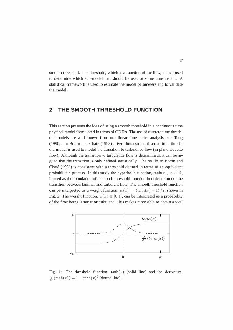
87
smooth threshold. The threshold, which is a function of the flow, is then usedto determine which sub-model that should be used at some time instant. Astatistical framework is used to estimate the model parameters and to validatethe model.
2 THE SMOOTH THRESHOLD FUNCTION
This section presents the idea of using a smooth threshold in a continuous timephysical model formulated in terms of ODE’s. The use of discrete time thresh-old models are well known from non-linear time series analysis, see Tong(1990). In Bottin and Chaté (1998) a two dimensional discrete time thresh-old model is used to model the transition to turbulence flow (in plane Couetteflow). Although the transition to turbulence flow is deterministic it can be ar-gued that the transition is only defined statistically. The results in Bottin andChaté (1998) is consistent with a threshold defined in terms of an equivalentprobabilistic process. In this study the hyperbolic function, tanh(x), x ∈ R,is used as the foundation of a smooth threshold function in order to model thetransition between laminar and turbulent flow. The smooth threshold functioncan be interpreted as a weight function,w(x) = (tanh(x) + 1) /2, shown inFig. 2. The weight function,w(x) ∈ [0 1], can be interpreted as a probabilityof the flow being laminar or turbulent. This makes it possible to obtain a total
tanh(x)
ddx (tanh(x))
x0
2
0
-2
Fig. 1: The threshold function, tanh(x) (solid line) and the derivative,ddt (tanh(x)) = 1 − tanh(x)2 (dotted line).

88
model,f , in terms of ODE’s on the form:
f = (1 −w(x)) f1(x,u,Θ, t) + w(x)f2(x,u,Θ, t),
wheref1 is a sub-model valid for laminar flow andf2 is a sub-model validfor turbulent flow. The vectoru contains the known inputs andΘ is a vec-tor of parameters. Finally, the weight function,w(x) is a function of thesystem states,x. The derivative of the weight function is continuous sinceddt (tanh(x)) = 1 − tanh(x)2, is continuous∀x ∈ R. Hereby, it should be pos-sible to formulate a total model which is continuous∀x ∈ R. The thresholdfunction and its first order derivative is shown in Fig. 1. Noww(x) is modifiedslightly:
w(x) = (tanh(a(x− b)) + 1) /2, (2)
wherea andb are scale and location parameters to be estimated. It is seen, thatthe threshold is now centered on the x-axis to a pointb and the shape is formedby the parametera. In the following section, a total model for the transientflow in a pipe based on the threshold model in Eq. (1), will be proposed.
(tanh(x)+1)2
x0
1
0
Fig. 2: The weight function,w(x) = (tanh(x)+1)2 .

89
3 DYNAMIC MODELLING OF PIPES
This section presents a lumped parameter model of the flow in a pipe, whereEq. (2) discussed in Section 2 is applied as a smooth threshold between twosub-models, one for laminar flow and one for turbulent flow. Using the secondlaw of Newton it easily follows that the flow,q, of an incompressible fluidout a pipe with the pressure drop,∆pp, can be determined by the first ordernon-linear differential equation:
dq
dt=A
l
(∆pp
ρ− (ψ +
λl
d)q2
2A2
), (3)
whereA is the cross-section area of the pipe with diameterd and lengthl, ρis the density of the water,ψ is the minor loss coefficient andλ is the frictionfactor. However, Eq. (3) is not valid for both laminar and turbulent flow, sincethe friction factor depends on the actual flow. For laminar flow the frictionfactor can be calculated using:
λ =64Re, Re=
ud
v, (4)
where Re is the Reynolds number,v is the kinematic viscosity of the fluid anduis the average speed of flow. For fully developed turbulent flow, the Colebrookformula (Fox and McDonald (1985)) holds:
1√λ
= −2log10
(γ
3.7d+
2.51Re
√λ
), (5)
whereγ is the absolute pipe roughness. Eq. (5) is transcendental and has to besolved by iteration. The turbulent region can be divided into smaller regions.For example, when the Reynolds number is less than1 · 105 and the pipe issmooth, the friction factor can be described by the Blasius equation (Fox andMcDonald (1985)):
λ =0.316Re0.25 . (6)

90
Reynolds number, Re
γ > 0
γ = 0
frictionfactorλ
Turbulentflow
2100
known
Laminarflow un-
2500
Fig. 3: Sketch of the friction factor as a function of the Reynolds number.
Reynolds number, Re
flowknownun- Turbulent
Smooththreshold
Laminarflow
Fig. 4: Sketch of the weight function as a function of the Reynolds number.
Depending on the physical properties of the actual pipe, such as the roughnessof the pipe, the flow in a pipe is known to be laminar for approximately Re≤2100 and turbulent for Re≥ 2500. In the region between,2100 ≤ Re≤ 2500,the flow is neither purely laminar nor purely turbulent, but a combination. Inthis interval, no expression for the friction factor,λ, exist. The friction factoras a function of the Reynolds number is sketched in Fig. 3. In the following thefriction factor at laminar and turbulent flow are denotedλl andλt, respectively.The sub-models describing the flow are written on the form Eq. (3) and denotedf1 for laminar flow andf2 for turbulent flow. Furthermore, the weight function,w(x) is a function of the Reynolds number, i.e.w(x) = w(Re), where:

91
w(Re) = (tanh(a(Re− b)) + 1) /2, (7)
wherea andb are parameters to be estimated. It should be noted, that the loca-tion parameterb is expected to be in the interval[2100; 2500]. To summarize,the model can be written:
dq
dt= (1 − w(Re)) f1(q,∆P ,Θ, t) + (w(Re)) f2(q,∆P ,Θ, t),
where the vectorΘ contains the model parameters:
Θ = [A, l, ρ, ... a, b]. (9)
4 PARAMETER ESTIMATION
In this section the parameter estimation method is discussed briefly. The sec-tion follows Melgaard (1994) closely. The total model is written:
dxt = f (xt,ut,Θ, t) dt, (10)
wherext is a vector of the system states and the vectorut contains the knowninputs. Finally,Θ is the vector of the parameters to be estimated. The model,Eq. (10), provides a deterministic description of the evolution in time of thestates of the system. It is obvious that any description of the form (10) givesonly an approximation of the evolution of the true system. In order to useEq. (10) as a description of the true variation of the states a stochastic term isincluded in Eq. (10) leading to the following stochastic differential equation:
dxt = f (xt,ut,Θ, t) dt+ g(Θ, t)dwt, (11)

92
wherewt is a Wiener process andg(Θ, t) is a function describing how thedisturbance is entering the system. Having measured some function of thestate variables, a state space representation can be formulated:
dxt = f (xt,ut,Θ, t) dt+ g(Θ, t)dwt, (12)
yt = h (xt,ut,Θ, t) + et, (13)
whereyt is a vector of the actually observed variables. Eq. (12) is a continuous-time system equation and Eq. (13) is the discrete time observation equation.The functionh describes the relationship between the state variablesxt andthe measurementsyt. Finally et is a vector describing the measurement noisewhich is assumed to be Gaussian distributed. The model parameters are foundusing discrete time observations of the pressure drop and flow, respectively.Let y = yk andu = uk denote the output/input sets of observations:
yk = [yk, yk−1, yk−1, ..., y1, y0], (14)
uk = [uk, uk−1, uk−1, ..., u1, u0], (15)
and letΘ be a vector of theN parameters to be estimated. The problem ofestimation is a matter of how to use the information contained in the data Eqs.(14-15) to select a proper valueΘ. In this study a Maximum Likelihood (ML)method is used to estimate the parameter vectorΘ. The conditioned likelihoodfunction is the joint probability density of all the observations assuming thatthe parameters are known (uk omitted for convenience):
L(Θ, yk) = p(yk|Θ) = p(yk|yk−1,Θ)p(yk−1,Θ)
=
(k∏
i=1
p(yi|yi−1,Θ)
), (16)
93
where Bayes rulep(A,B) = p(A|B)p(B) is applied. It is now assumed thatthe sequence of innovations,εk, are zero-mean, independent stochastic vari-ables with the probability density functionp(ε(Θ)). Then, Eq. (16) can beformulated:
L(Θ, yk) =
(k∏
i=1
p(εi(Θ))
). (17)
The ML estimates,ΘML, is found by minimizing the function−logL(Θ, yk):
ΘML = arg minΘ
(−
k∑i=1
log p(εi(Θ))
). (18)
When the prediction errors are assumed to be Gaussian with zero mean, andcovariance matrixRk(Θ), then
−logL(Θ, yk) =12
k∑i=1
(ε>i R−1k εi + log detRi + s log2π). (19)
wheres is the dimension ofy. It should be noted that if the assumption thatthe prediction errors are Gaussian distributed, the method can be consideredas a prediction error method. The estimated model is validated using phys-ical interpretation and statistical methods, such as prediction errors analysis,simulation studies and cross validation.
5 THE EXPERIMENTAL SETUP
In order to collect data for the modeling and validation process of the transientflow an experimental setup was built at the Danish Technological Institute. Theexperimental setup is sketched in Fig. 5. During the experiment the pressuredrop ∆P [Pa], the flowq [m3/s] as well as the inlet and the outlet temper-atures[◦C] were measured. Using a Moody’s diagram the dimensions of the

94
pipe were selected to be 12.0/0.01 (length/diameter[m]) in order to be able togenerate both laminar and turbulent flow. The pipe material was made of softcopper and winded up to avoid sharp edges. Finally, a computer was used tocontrol the flow as well as the inlet temperature.
Pressure DropTemperature censorsValves
Fig. 5: Sketch of the experimental setup.
6 THE DATA
The preliminary analysis of the experimental setup yield that the transient flowwill appear for Reynolds numbers in the interval[2100 ; 2500]. This corre-sponds to a flow in the interval[65 ; 75] [kg/h] when the supply temperature
Pressure drop∆P [kPa]
Flow q [kg/h]806050
2
0
Fig. 6: Phase diagram of the pressure drop∆P vs. the flowq.

95
Pressure drop∆P [kPa]
time [sec.]10005000
4
2
0
Flow q [kg/h]
time [sec.]10005000
120
80
40
0
Fig. 7: The measured pressure drop and corresponding flow in a type (iii)experiment.
of the water,Ts is 30[◦C]. This assumption is supported by the phase diagramin Fig. 6, obtained from a preliminary steady state experiment. Furthermore,a hysteresis effect is seen in this interval, corresponding to that the transitionfrom laminar to turbulent flow occurs at a higher flow rate than the transitionfrom turbulent to laminar flow, respectively.
Several controlled dynamical experiments were performed using different lev-els of flow and constant supply temperature. The experiments can be catego-rized into the following three groups:
(i) q : 10 20 30 40 [kg/h] andTs : 30 [◦C].
(ii) q : 90 110 130 150 [kg/h] andTs : 30 [◦C].
(iii) q : 20 60 100 140 [kg/h] andTs : 30 [◦C].

96
where (i) is a dynamical experiment in the laminar region, (ii) is a dynamicalexperiment in the turbulent region and finally the dynamical experiment (iii)is covering both regions, including the transient region. The sample frequencyof the experiments, cf. above, was 1 Hz. In Fig. 7 a sample time series ofthe pressure drop and the flow is shown for the type (iii) experiment, i.e. bothlaminar, transient and turbulent flow occurs.
7 RESULTS
The sub-models for laminar and turbulent flow were estimated using type (i)and (ii) experimental data. Eq. (4) and Eq. (6) were applied forλl andλt,respectively, and the first order non-linear model Eq. (3) was found adequatein both regions. Finally, the total model was written on the form Eq. (1) andtype (iii) experimental data was used for parameter estimation. Since most ofthe model parameters, such as the pipe diameter, the length and the minor lossconstant were either known or estimates directly in the sub-models, only the(most interesting) parametersa, b, the initial stateq0 and the noise terms hadto be estimated. To ensure that the parameter estimates converges towards theglobal supremum for the likelihood function, several estimations using differ-ent initial values of the parameters were performed. In Fig. 8 the estimatedautocorrelation function for the model residuals are shown. It is concludedthat the residuals can be considered as being Gaussian white noise and thus
Lagk20101
0.04
-0.04
0
Fig. 8: The estimated autocorrelation function for the residuals.

97
Measured flow vs. Simulated Flow[kg/h]
time [sec.]5000
120
80
40
0
Fig. 9: Cross validation. The model is used to simulate the system using astochastic independent time series. Simulated (solid line) and measured (dottedline).
105
Value ofb7570656055504540
-2.10
-2.15
-2.20
Fig. 10: The profile likelihood for the parameterb. The optimal value is foundfor b = 48 [kg/h].
that the model describes the dynamics of the system. Hence, statistically itis concluded that a reasonable model is found. The reasonable performanceof the model is supported by the cross validation study, shown in Fig. 9. Theoptimum value of the parameterb, which is the value wherew(x) = 0.5, isfound to beb = 48 [kg/h]. The profile likelihood is shown in Fig. 10. Theestimated value ofb is smaller than first expected compared with the phasediagram in Fig. 6, which was obtained for steady state experiments. It can beargued, as in Bottin and Chaté (1998), that all turbulence has to vanish beforethe flow is purely laminar. Thus, during the dynamical experiment the flow has
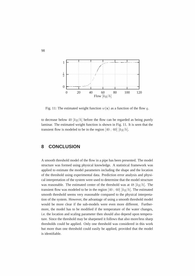
98
Flow [kg/h]120100806040200
1
12
0
Fig. 11: The estimated weight functionw(x) as a function of the flowq.
to decrease below40 [kg/h] before the flow can be regarded as being purelylaminar. The estimated weight function is shown in Fig. 11. It is seen that thetransient flow is modeled to be in the region[40 ; 60] [kg/h].
8 CONCLUSION
A smooth threshold model of the flow in a pipe has been presented. The modelstructure was formed using physical knowledge. A statistical framework wasapplied to estimate the model parameters including the shape and the locationof the threshold using experimental data. Prediction error analysis and physi-cal interpretation of the system were used to determine that the model structurewas reasonable. The estimated center of the threshold was at48 [kg/h]. Thetransient flow was modeled to be in the region[40 ; 60] [kg/h]. The estimatedsmooth threshold seems very reasonable compared to the physical interpreta-tion of the system. However, the advantage of using a smooth threshold modelwould be more clear if the sub-models were even more different. Further-more, the model has to be modified if the temperature of the water changes,i.e. the location and scaling parameter then should also depend upon tempera-ture. Since the threshold may be sharpened it follows that also more/less sharpthresholds could be applied. Only one threshold was considered in this workbut more than one threshold could easily be applied, provided that the modelis identifiable.

Paper D
A MODEL FOR THE HEATDYNAMICS OF A RADIATOR
D
99


101
ABSTRACT
A model of the heat dynamics of a panel radiator is presented. The model isobtained from physical reasoning and experimental data. The model is lumpedinto two compartments and the size of these compartments depends on theactual flow. By introduction of variable compartment sizes, it is shown that itis possible to keep the model order low and obtain a very accurate model whencompared to empirical data. The model is formulated in continuous time, usingstochastic differential equations which make it directly physical interpretable.Statistical methods are used for parameter estimation and model validation.The simulation performance of the model is illustrated.
Keywords:Radiators, heat dynamics, lumped parameter modelling, grey boxmodelling method.
1 INTRODUCTION
There is a need for development of dynamic models of water based centralheating systems in order to analyze and interpret the physical interaction be-tween system components, such as radiators, valves, heat exchangers etc. Suchmodels can be useful e.g. in the design of control systems containing feedbackloops. A radiator is a typical component in a water based central heating sys-tem. It is a distributed system for which the dynamics in principle may bedescribed by physical laws concerning mass, energy and momentum. In thispaper a model describing the heat dynamics of a radiator is proposed combin-ing physical knowledge and statistical methods.
Different modeling techniques have been applied to model the dynamics ofcomponents in water based central heating systems, see e.g. Jonsson (1990);Sejling (1993); Hansen (1997); Bourdouxhe et al. (1998). The dynamics ofthe components and the interactions between these can be described by con-sidering the thermal and hydraulic characteristics of the system. However, theamount of literature on dynamic modelling of radiators is sparse.
102
Various steady state models of radiators can be found in the literature, seee.g. Benonysson (1991). Such steady state models are in Madsen and Holst(1995) and in Andersen et al. (2000) found adequate in deriving a total modelof the heat dynamics in a building. A possible approach towards obtaininga dynamic model is to lump the radiator into compartments, and formulate adynamic model based upon laws of heat transfer. The energy balance of eachcompartment is then expressed in terms of ordinary differential equations. Thisapproach is used in Paulsen and Grundtoft (1985), where the radiator is dividedintoN equally sized compartments. The energy balance of each compartmentis calculated using ’handbook’ parameters. Based on experiments and simula-tions it is found, that the best performance is obtained when selectingN in therange 10-20 compartments. A drawback using this approach is that the modelorder becomes rather high. The large number of compartments is found nec-essary to avoid numeric diffusion, i.e., the temperature ’moves’ faster than theflow, which is a non-physical property. In Hansen (1997), a stochastic mod-elling approach, the grey box modelling method, is applied to model the heatdynamics of a radiator. The grey box modeling method is characterized byusing both physical knowledge and information from data in determining anadequate model structure. The proposed model is lumped into a number ofequally sized compartments. The model structure is identified using physicallaws as well as measurements from an experimental setup. Statistical methodsare used to determine the model parameterization and the optimal number ofcompartments is found to be two for the particular experimental setup. How-ever, applying statistical test indicates that the model parameterization is in-adequate. It is concluded in Hansen (1997) that the model structure has to beimproved.
In this paper a new model parameterization is proposed using the grey boxmodeling approach. The grey box modelling approach has earlier been appliedfor various other components in water based central heating systems, see e.g.Jonsson et al. (1992); Jonsson and Palsson (1992, 1994); Hansen (1997); An-dersen et al. (2000). For detailed discussion on the grey box modeling method,see Tulleken (1992, 1993); Melgaard (1994); Ljung and Glad (1994). Themodel presented in this paper is also a lumped parameter model, but the basicidea is that the compartmental sizes may vary, depending on the flow. Thiscorresponds better to the distribution of the temperature of the water and ra-

103
diator material, which can be observed using thermo-vision (Adunka (1992)).The heat dynamics of the compartments are modelled by considering the en-ergy balances. The heat transfer to the air surrounding the radiator surface ismodelled using a similar dependency. Finally, the variation of the section sizesis modelled. The suggested model describes the heat dynamics when excitedby different input signals, such as changes in the flow controlled by a thermo-static valve and variations in the ambient air temperature. Statistical methodsare used to determine estimate the significant model parameters and to validatethe model structure.
2 THE MODELLING APPROACH
In this section the applied modelling approach is briefly described. The greybox modelling method is selected since it is a suitable approach in combiningphysical knowledge and experimental data in the modelling process, see e.g.Tulleken (1992, 1993); Melgaard (1994); Ljung and Glad (1994). Physicalknowledge is used in forming the model structure, but the modelling is keptin a stochastic framework and statistical methods are applied in determiningthe parameters of the model. The model is formulated in continuous time andexpressed in terms of stochastic differential equations. Both the states andthe parameters of the model are estimated using a Maximum Likelihood (ML)method. Finally, the model is validated using both statistical methods andphysical knowledge. This modelling approach may be preferable compared toa deterministic modelling approach because the physical system to be modelledis only known partly and model approximations are inevitable. The grey boxmodelling method complies with these difficulties, using statistical methods todetermine whether or not the model parameterization is adequate, and if not,how to improve the model.
To model the impact from the assumingly most important variables on the heatdynamics of the radiator, well known thermo dynamic relationships are used,and formulated in terms of a system of ordinary differential equations:

104
dXdt
= f (X,U, θ, t) , (1)
whereX is a vector of system states and the vectorU contains the known in-puts. Finally,θ is a vector of parameters. The lumped model, Eq. (1), providesa deterministic description of the evolution in time of the states of the system.It is obvious that any description of the form (1) only yields an approximationof the evolution of the true system. In order to use Eq. (1) as the foundationfor a description of the true variation of the states a stochastic term is includedin Eq. (1) leading to the following system of stochastic differential equations:
dXdt
= f (X,U, θ, t) + G(θ, t)dW, (2)
whereW is a Wiener process withE[dW]2 = dt and G(θ, t) is a func-tion describing how the disturbance is entering the system. For a discussionon stochastic differential equations, see e.g. Kloeden et al. (1997); Øksendal(1985); Risken (1996). There are several reasons for introducing a noise termin Eq. (1), referring to Melgaard (1994):
• Modeling approximations. The system described by Eq. (1) might be anapproximation to the true system.
• Unrecognized and unmodelled inputs may affect the evolution of thestates.
• Measurements of the input are noise-corrupted.
Having measured some function of the state variables, a state space represen-tation can be formulated:
dXdt
= f (X,U, θ, t) + G(θ, t)dW, (3)
Y = h (X,U, θ, t) + et, (4)
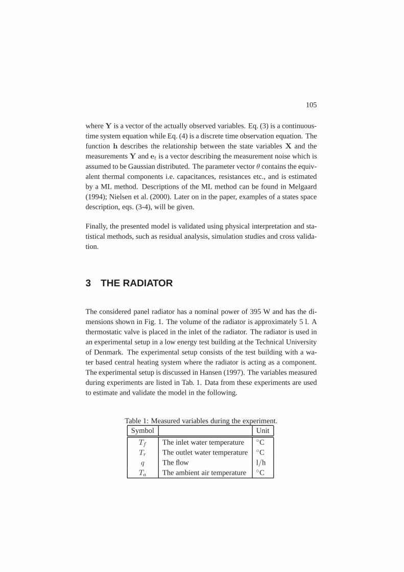
105
whereY is a vector of the actually observed variables. Eq. (3) is a continuous-time system equation while Eq. (4) is a discrete time observation equation. Thefunction h describes the relationship between the state variablesX and themeasurementsY andet is a vector describing the measurement noise which isassumed to be Gaussian distributed. The parameter vectorθ contains the equiv-alent thermal components i.e. capacitances, resistances etc., and is estimatedby a ML method. Descriptions of the ML method can be found in Melgaard(1994); Nielsen et al. (2000). Later on in the paper, examples of a states spacedescription, eqs. (3-4), will be given.
Finally, the presented model is validated using physical interpretation and sta-tistical methods, such as residual analysis, simulation studies and cross valida-tion.
3 THE RADIATOR
The considered panel radiator has a nominal power of 395 W and has the di-mensions shown in Fig. 1. The volume of the radiator is approximately 5 l. Athermostatic valve is placed in the inlet of the radiator. The radiator is used inan experimental setup in a low energy test building at the Technical Universityof Denmark. The experimental setup consists of the test building with a wa-ter based central heating system where the radiator is acting as a component.The experimental setup is discussed in Hansen (1997). The variables measuredduring experiments are listed in Tab. 1. Data from these experiments are usedto estimate and validate the model in the following.
Table 1: Measured variables during the experiment.Symbol Unit
Tf The inlet water temperature ◦CTr The outlet water temperature◦Cq The flow l/hTa The ambient air temperature ◦C
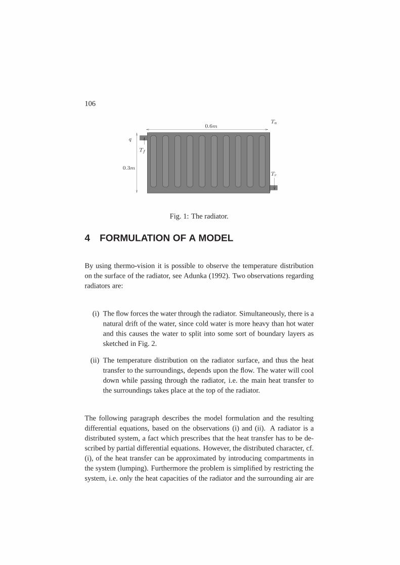
106
Tr
Ta
Tf
q
0.3m
0.6m
Fig. 1: The radiator.
4 FORMULATION OF A MODEL
By using thermo-vision it is possible to observe the temperature distributionon the surface of the radiator, see Adunka (1992). Two observations regardingradiators are:
(i) The flow forces the water through the radiator. Simultaneously, there is anatural drift of the water, since cold water is more heavy than hot waterand this causes the water to split into some sort of boundary layers assketched in Fig. 2.
(ii) The temperature distribution on the radiator surface, and thus the heattransfer to the surroundings, depends upon the flow. The water will cooldown while passing through the radiator, i.e. the main heat transfer tothe surroundings takes place at the top of the radiator.
The following paragraph describes the model formulation and the resultingdifferential equations, based on the observations (i) and (ii). A radiator is adistributed system, a fact which prescribes that the heat transfer has to be de-scribed by partial differential equations. However, the distributed character, cf.(i), of the heat transfer can be approximated by introducing compartments inthe system (lumping). Furthermore the problem is simplified by restricting thesystem, i.e. only the heat capacities of the radiator and the surrounding air are

107
Tf
T1
T2
Tr
q
Fig. 2: A sketch of the assumed drift of water in the radiator.
modelled. An interpretation of the modelling approach is sketched in Fig. 3.The radiator is lumped into 2 compartments where the temperature is assumedconstant. The energy balance of each element is considered and this includesa description of the surrounding air. Finally, the size of each compartmentdepends on the flow.
Referring to Fig. 3 it is assumed that the water in each compartment is perfectlymixed and that the fluid properties are constant. The assumption that the radia-tor can be lumped into perfectly mixed compartments can be be validated usingsteady state measurements Paulsen and Grundtoft (1985). The assumption thatthe fluid properties are constant is reasonable since the variations in the inlet
A
T`
T2
T1 (1 −A)
Fig. 3: The lumped model. The radiator is divided into two compartments.The size of the compartments depend on the flow.

108
temperature of such a radiator is typically in the interval 40-60◦C. Thus thedensity and the specific heat of the water are estimated to vary relatively lessthan 1 and 0.1 %, respectively. Finally, it is assumed that the water and the ra-diator material are incompressible. The temperatures of the two compartmentsare denotedT1 andT2, respectively. The temperature of the surrounding air isdenotedT`. The functional area of the upper compartment is denotedA andthe lower compartment(1 − A), whereA ∈]0 1[. Furthermore it is assumed,that the temperature of the metal in each compartment equals the temperatureof the water, i.e.T1 andT2, respectively. The energy balance is written in termsof ordinary differential equations. In general as:
dQstored
dt=∑
Φin −∑
Φout, (5)
whereΦin/out denotes the input/output power, anddQ/dt denotes the timederivative of the energyQ(t).
The heat capacity of each section is denotedC1 andC2, respectively. By in-troducing the heat capacity of the entire radiator,Cr, implies that:
C1 = CrA and C2 = Cr(1 −A). (6)
The heat balance Eq. (5) of the upper compartment becomes:
CrAdT1
dt= kq(Tf − T1) − kq(T1 − T2) −HrA(T1 − T`)n, (7)
wherek is the product of the specific heat capacity, the density of the waterand the radiator material.Hr is the heat transfer coefficient from the radiatorto the surrounding air with temperatureT` andn denotes the radiator exponent.Similar, the heat balance of the lower section becomes:
Cr(1 −A)dT2
dt= kq(T1 − T2) −Hr(1 −A)(T2 − T`)n, (8)
where the temperatureT2 is taken to be equal to the return temperature. Con-sidering the heat transfer from the radiator to the room air, an approximationto the energy balance of the surrounding air becomes:

109
C`dT`
dt= HrA(T1 − T`)n +Hr(1 −A)(T2 − T`)n −B`(T` − Ta), (9)
whereB` is the heat transmission coefficient to the ambient air with tempera-tureTa. Finally the variation in time of the section areas need to be modelled.The upper section areaA, and thus the lower section area(1 − A), will bemodelled as:
dA
dt= aq − bA, (10)
wherea andb are parameters to be estimated, andq is the flow. Equation (10)states that when the flow increases the area of the upper compartment increaseas well. The latter term on the right hand side of (10) leads to an exponen-tial decrease of the upper area if the flow at some time instant becomes small.This corresponds to the physical interpretation of the drift of the hot water inthe radiator. Furthermore it should be noted, that since the flow is restricted,constraints are put on the parametersa andb so that the areaA is restricted tobe in the intervalA ∈]0 1[. Equation 10 is a very simple expression for howthe compartment sizes may vary. If the statistical analysis indicates that thisdescription is not sufficient, Eq. 10 can be extended to include the fluid prop-erties and the structure of the radiator as well as the flow. The appropriatenessof Eq. 10 will be examined in the subsequent section.
In summary, the heat dynamics of the radiator is modelled by the four cou-pled non-linear ordinary differential equations, Eq. (7-10). The temperature ineach compartment, the surrounding air temperature and the compartment sizesare taken as state variables. The flow, the inlet temperature and the ambientair temperature are input variables. By introducing additive noise, and regard-ing the states and parameters as stochastic variables, the set of equations, Eq.(7-10), forms the system equation, Eq. (3). Having measured the outlet tem-perature,Tr, the observation equation, Eq. (4) becomes:
Tr = T2 + e1. (11)

110
The total model is given in the appendix, eqs. (12-16).
The system equationdXt = f(X(t),U(t), θ, t)dt + G(θ, t)dWt:
dT1
dt=
kq
CrA(Tf − 2T1 + T2) − Hr
Cr(T1 − T`)n + dω1 (12)
dT2
dt=
kq
Cr(1 −A)(T1 − T2) − Hr
Cr(T2 − T`)n + dω2 (13)
dT`
dt=Hr
C`A(T1 − T`)n +
Hr
C`(1 −A)(T2 − T`)n − B`
C`(T` − Ta) + dω3
(14)
dA
dt= aq − bA+ dω4. (15)
The observation equationYk = h(X(t),U(t), θ, t) + e(t):
Tr = T2 + et. (16)
5 RESULTS
In this section the results from the modelling procedure are given. The re-sults are based on 1000 observations with sampling time of 1 min. from theexperiment described in section 3. The state variables and the parameters havebeen estimated using the ML method. The model is validated using statisticalmethods to support the physical interpretation of the model states. Finally, thesimulation performance of the system is illustrated and the model is validatedon a stochastic independent time series.
In Tab. 2 the estimated model parameters and their standard deviation are pre-sented. The parameter estimates, which are directly physically interpretable,seems reasonable validated to handbook parameters. Since the model parame-ters are directly physical interpretable they can be used in simulation studies,e.g. as design parameters for control strategies. Furthermore, the model statesmay also be given a physical interpretation. The water and the air temperaturesare shown in Fig. 4. The estimated values of the states agree with the physical

111
Table 2: Estimates of model parameters.Symbol Estimate Std. deviation Unit
Cr 3.01 0.05 kJ/K
Hr 49.06 4.36 kJ/(Kh)C` 0.90 0.08 kJ/K
B` 9.73 0.42 kJ/(Kh)a 6.410−2 6.4410−3 m2/(l/h)b 1.410−2 6.2410−3 1/h
interpretation, namely that the water is cooling down and the surrounding airis heated. Thus, the model may be used to simulate the unobserved states ofthe radiator.
The estimated compartment sizes and the measured flow are shown in Fig. 5.The variations in the flow are inducted by a thermostatic valve (slow variation)as well as a pump switching between two operating points. It is seen that the
0 100 200 300 400 500 600 700 800 900 100046
48
50
52
54
56
58
0 100 200 300 400 500 600 700 800 900 100020
22
24
26
28
30
32
◦C
◦C T1
Tf
T2
T`
Ta
time (minutes)
Fig. 4: Top: Water temperatures. Bottom: Air temperatures.

112
compartment sizes as expected depend on the variations in the flow.
0 100 200 300 400 500 600 700 800 900 100074
76
78
80
82
84
0 100 200 300 400 500 600 700 800 900 100010
15
20
25
lh
% A
q
A
1 −A
time (minutes)
Fig. 5: Top: Estimated sizes of the compartments. Bottom: Measured flow.
It is found that the model is able to predict the return temperature with a highaccuracy, i.e. the prediction errors, or the model residuals, are very small. Thepredicted return temperature are not shown, since it is not possible to distin-guish the predicted temperature from the true observations in a plot. In Fig. 6the cumulated periodogram of the residuals is shown. It is concluded, that themodel residuals can be accepted as being white noise, i.e. the model describesall the observed dynamics of the system. The simulation performance of themodel is presented in Fig. 7. It is seen that the model is able to simulate thesystem very accurately and the simulation performance is therefore consideredsatisfactory. Finally, a cross validation on an independent time series has beenperformed and is presented in Fig. 8. It is seen that the model agrees nicelywith the measured time series. From this statistical analysis it is concludedthat it is not necessary to extend the model further in order to model the heatdynamics of the radiator.

113
0 0.05 0.1 0.15 0.2 0.25 0.3 0.35 0.4 0.45 0.50
0.1
0.2
0.3
0.4
0.5
0.6
0.7
0.8
0.9
1
Fig. 6: Normalized accumulated periodogram
0 100 200 300 400 500 600 700 800 900 100046
47
48
49
50
51
52
53
54
◦CT2
Tr
time (minutes)
Fig. 7: Simulation of the return temperatureTr.
6 CONCLUSION
A lumped parameter model for the heat dynamics of a radiator has been pro-posed. Both physical knowledge and experimental data have been used informulating the model structure. It was argued, that the compartment sizes in alumped parameter model should be a function of the actual flow. The variationin the size of the compartments could be interpreted as how the flow influ-ences the temperature distribution and the drift of the water in the radiator, afact which can be observed using thermo-vision. Introducing the compartmentsize as a state variable, it was possible to model the variation of the compart-ment sizes. This further implied, that since the lumping of the radiator wasdependent upon the flow, it was possible to reduce the model order signifi-
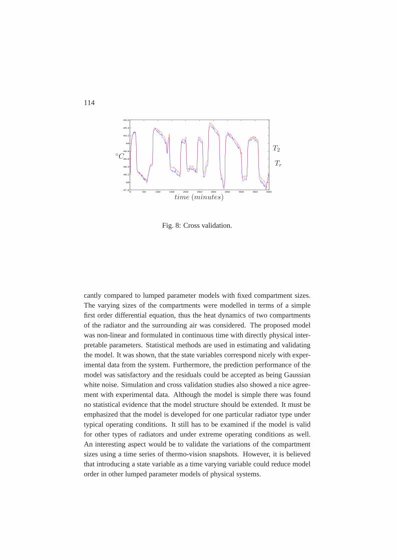
114
0 50 100 150 200 250 300 350 400 450 50047.8
48
48.2
48.4
48.6
48.8
49
49.2
49.4
49.6
◦CT2
Tr
time (minutes)
Fig. 8: Cross validation.
cantly compared to lumped parameter models with fixed compartment sizes.The varying sizes of the compartments were modelled in terms of a simplefirst order differential equation, thus the heat dynamics of two compartmentsof the radiator and the surrounding air was considered. The proposed modelwas non-linear and formulated in continuous time with directly physical inter-pretable parameters. Statistical methods are used in estimating and validatingthe model. It was shown, that the state variables correspond nicely with exper-imental data from the system. Furthermore, the prediction performance of themodel was satisfactory and the residuals could be accepted as being Gaussianwhite noise. Simulation and cross validation studies also showed a nice agree-ment with experimental data. Although the model is simple there was foundno statistical evidence that the model structure should be extended. It must beemphasized that the model is developed for one particular radiator type undertypical operating conditions. It still has to be examined if the model is validfor other types of radiators and under extreme operating conditions as well.An interesting aspect would be to validate the variations of the compartmentsizes using a time series of thermo-vision snapshots. However, it is believedthat introducing a state variable as a time varying variable could reduce modelorder in other lumped parameter models of physical systems.

115
NOMENCLATURE
Symbol Unit
A Area of upper compartment %m2
B` Conductivity coeff. kJ/(Kh)C` Heat capacity of ambient air kJ/K
Cr Heat capacity of radiator kJ/K
Hr Conductivity coeff. kJ/(Kh)Ta Ambient air temperature ◦CTf Supply water temperature ◦CT1 Temperature of upper compartment◦CT2 Temperature of lower compartment◦CT` Ambient air temperatur ◦CTr Return temperature ◦Ca Radiator parameter m2/(l/h)b Radiator parameter l/h
dw(·) System error ◦Ce(·) Measurement error ◦Ck Constantn Radiator exponent −q Flow l/h

116

Paper E
MODELLING OF ATHERMOSTATIC VALVE
WITH HYSTERESISEFFECTS
E
117


119
ABSTRACT
This paper presents a model of a thermostatic valve based on first principlesand where the hysteresis effect is modeled using an adaptive model for frictioncompensation. The grey box modeling approach is applied, i.e. both physicalinterpretation and statistical methods are used to build and validate the sug-gested model. The model performance is illustrated using empirical data andissues concerning the modeling of hysteresis in valves are discussed.
Keywords: Thermostatic Valve, Hysteresis effects, Friction, Grey box model-ing, Statistical methods.
1 INTRODUCTION
The use of mathematical models as a means for simulation of heating systemshas improved both the understanding and the capability of controlling suchsystems. The importance of developing and applying adequate mathematicalmodels has increased since the focal point in product development has changedfrom focusing on the component (sub optimization) to focusing on the interac-tions of the components (system optimization). Today, a large part of productdevelopment can be done by computer simulation as a replacement for the tra-ditional in situ testing, which for complex systems is both expensive and timeconsuming.
The introduction of thermostatic valves in residential buildings during the lastdecades has significantly reduced the energy consumption and improved thethermal comfort. Today the thermostatic valve is a standard component in mostwater based heating systems. In this study a model for a thermostatic valve ispresented. A major difficulty in the modeling thermostatic valves is the highlynon-linear effect from hysteresis. We propose to use a dynamic model basedon physical interpretation and first principles (force balances) in combinationwith an adaptive friction model to deal with this problem. The resulting modelis characterized as a grey box model due to the combination of using first prin-

120
ciples and empirical methods. The unknown terms of the model are estimatedusing statistical methods and experimental data, whereas the model is validatedusing both physical interpretation and statistical methods.
2 THE MODELLING OF THERMOSTATIC VALVES
The thermostatic valve considered in this study is typically used for tempera-ture control of small hot water cylinders (e.g. storage tanks) or heat exchang-ers in radiator heating systems. It is a self-acting thermostatic valve, where agas ampoule in the thermostat will increase/decrease the pressure on the valvecone as the surrounding temperature increases/decreases and force the valve toclose/open.
Since the thermostatic valve is common in heating system installations it isimportant to develop adequate models, e.g. for design of control strategies andproduct development. There exist extensive literature on mathematical modelsof both thermostats and valves separately as well as models of thermostaticvalves, see e.g. Hansen (1997); Bourdouxhe et al. (1998); Zou et al. (1999);Kayihan (2000). The purpose of these models is primarily to optimize thecontrol of heating and cooling systems. The mathematical modeling, however,is not straight-forward due to strong non-linear factors such as hysteresis. Thepurpose of this study is to develop a model that is directly physical interpretableand able to handle the non-linearities.
To obtain an adequate physical model we propose to use the grey box modelingapproach in modeling the thermostatic valve. The grey box modeling approachis characterized by using both prior knowledge, such as physical laws, as wellas information from empirical data in the identification procedure. The advan-tage of this approach is that the model may be given a physical interpretationas well as non-linear effects may be more effectively described compared toa black box model. On the other hand, the use of empirical data provides formore adequate models compared to a pure deterministic or white-box model.The grey box method will not be discussed in detail in this paper. For a dis-cussion on grey box modeling approaches, see Tulleken (1992); Ljung and

121
Glad (1994); Melgaard (1994). For grey box applications of components inheating systems, see e.g. Jonsson and Palsson (1994); Weyer et al. (2000) forheat exchanger modeling, Madsen and Holst (1995) for modeling building heatdynamics, and Gordon et al. (2000) for modeling of air conditioners.
3 THE MODEL FORMULATION
In this section a model of the valve will be proposed. The model is basedon physical interpretation and first principles. A simplified sketch of the ther-mostatic valve is shown in Fig. 1, emphasizing the mechanical parts. Arrowsindicate the direction of the forces, which influences on the mechanical parts.Note that only forces that are considered significant are sketched. These are inparticular the force from the thermostat (via the spring), friction in the valveand the forces due to the differential pressure as well as the velocity of theliquid through the valve opening.
3.1 Formulation of the force balance
In the following each of the considered forces that is assumed to affect thevalve will be formulated in mathematical terms. Based on this a force balancewill be proposed. It should be emphasized that the sign of the various forcesare indicated by the arrows in Fig. 1, assuming that the forces are positivewhen considered from the right. The force balance is given as the sum of theconsidered forces:
−Ff + Fp + Fs − Fg + Fv + Fi − Fb ± Fh = 0, (1)
where the terms are explained in Fig. 1. In the following each term will beconsidered more closely. The flow forces,Ff can be interpreted as a springforceKf∆pk that are trying to close the valve:

122
p0 Atmospheric pressure
p1 Pressure at inlet
p2 Pressure at outlet
SP Fix point
x Valve opening
Ff Flow forces
Fp Differential pressure at valve cone
Fs Differential pressure at stem/spindle
Fh Friction
Fv Valve spring
Fi Setting spring
Fg Differential pressure at bellows
Fb Bellows spring
Fig. 1: Sketch of the thermostatic valve. The shaded area surroundingpq indi-cates the gas chamber, while the arrows atp1 andp2 indicates the upstream anddownstream pressure. The nomenclature for the various parameters are givenin the table below the sketch.
Ff = Kf · x · ∆pk, (2)
where∆pk is the differential pressure at the cone,Kf is a constant andx is the

123
valve opening. The forces due to the differential pressure are defined from thearea on which they are affecting:
Fp = Ak(p1 − p2) = Ak · ∆pk. (3)
Fs = As(p1 − p0) = As · ∆ps. (4)
Fg = Ab(pg − p0) = Ab · ∆pb(Tg). (5)
Ak, As andAb are the area of the cone, the spindle and the bellows, respec-tively. The differential pressure is dependent of the temperature of the gasinside the thermostat,Tg, which determines the pressure of the gaspb. Thespring forces, i.e. the forces from the valve spring, the setting spring and thebellows spring, are defined from Hooks law, which is a linear function of thevalve position:
Fv = Fv0 − Cv · x. (6)
Fi = Fi0 − Ci · x. (7)
Fb = Fb0 + Cb · x. (8)
Fv0,i0,b0 andCv,i,b are constants. The force due to friction,±Fh, is workingagainst the velocity of the valve and hereby a cause to hysteresis. Since itis not straight-forward to define this friction force, an adaptive model will beintroduced in Section 3.2 to model for the friction force. If the valve openingis set equal tox = 0 in (10), four fix-point values(SP ) are given as:
Ak ·∆pk,SP +As ·∆ps,SP +Fv0 +Fi,SP −Ab ·∆pb(Tg,SP )−Fb0 = 0. (9)
In this expression the force from fiction is neglected. The fix-point values areconstant and depend only on the actual calibration (set-points) of the thermo-static valve. Now, the force balance can be written as Eq. (10):

124
−Kf · x · ∆pk +Ak · ∆pk +As · ∆ps −Ab · ∆pb(Tg)
+(Fv0 −Cv · x
)+(Fi0 − Ci · x
)− (Fb0 + Cb · x)± Fh = 0.
(10)
By isolating the valve positionx we obtain:
x =Ak
(∆pk−∆pk,SP
)+As
(∆ps−∆ps,SP
)−Ab
(∆pb(Tg)−∆pb(Tg,SP )
)±Fh
Cv+Ci+Cb+Kf∆pk. (11)
In the following the modeling of the hysteresis force±Fh will be discussed.
3.2 Models of hysteresis
This section discusses the modeling of the hysteresis force,±Fh. Hysteresisis a phenomenon that appears in many mechanical and electrical systems, in-cluding thermostatic valves. The hysteresis force is characterized by the factthat the valve position is a function of local phenomena such as the gradient ofthe velocity of the stem. The hysteresis effect is a significant factor in the mod-eling of thermostatic valves and it is considered important to account for thisin the model which objective is for prediction and control purposes. In section4 the effects of hysteresis on the thermostatic valve will be visualized usingempirical data. In the following some modeling approaches for hysteresis willbe discussed. Emphasis will be put on a model proposed in Dahl (1968) thatwill be included in the total model of the thermostatic valve.
The play model
A very simple model of hysteresis is the‘play model’, see e.g. (Visintin (1994);Cahlon et al. (1997)). It is defined as two functions that separates the hystere-sis region, which typically looks like the phase diagram shown in Fig. 2. If thetemperature of the valve is decreasing the valve position will be described by

125
the slope of the left side of the region. If the temperature is increasing the posi-tion is determined by the slope on the right side of the region. If the gradient ofthe temperature is changing the model will switch to the appropriate slope. Insuch a situation the valve position will not change and the movement betweenthe two slopes will be horizontal.
Temperature
Val
ve O
peni
ng
Fig. 2: Sketch of the‘play model’.
It is obvious that the play model is a rough approximation and a pure black boxmodel of the hysteresis, i.e. no physical interpretation is accounted for.
Dahl’s model
A more detailed model is the Dahl model. It is a commonly used model fordescribing forces arising from frictionFh and described in Dahl (1968). Themodel states the relationship between the stretch and strain of a given material.The Dahl model was originally developed for simulation of control systemswith friction. The model may however be used for other applications, e.g.in adaptive friction compensation, see Olsson et al. (1997). This is also thepurpose of the Dahl model in this study. Let the friction force be defined asF ,the Coulomb’s friction force asFc and the displacement asx. Dahl’s modelhas then the form:
dF
dx= σ
(1 − F
Fcsgn(v)
)α, (12)

126
F
F
- F
c
c
x
x > 0.
x < 0.
σ0
Fig. 3: Sketch of the friction forceF as a function of the dissaplacementx.
whereσ denotes the elasticity, andα is the slope of the movement. A sketchof the model is shown in Fig. 3. It is seen that the friction force is solelydefined from the length of the displacement and its direction,sgn(v). Herebythe possibility of static friction nor the Stribeck effect is not considered in themodel (Olsson et al. (1997)). In Fig. 3 it is shown that as the displacementincrease the friction force will equal the Coulomb’s friction forceFc, and thusthe maximal friction force for both negative and positive displacement, i.e.|F | ≤ Fc. By changing the direction of the movement the curve is flipped overand the maximal friction force is then−Fc. The slope forF = 0 is indicatedasσ0.
The Dahl model can be reformulated for the time domain, see Olsson et al.(1997):
dF
dt=dF
dx
dx
dt=dF
dxv = σ
(1 − F
Fcsgn(v)
)αv, (13)
which results in a first order non-linear differential equation.

127
Using the Dahl model for the valve hysteresis
This section describes how the Dahl model will be used to model the frictionforce,Fh, in the model of the valve Eq. (11). Since Dahl’s model directly givesthe friction force as a function of the displacement it seems obvious to use thethe valve position asx. This gives some difficulties, however, since the purposeof the model is to predict the valve position, but then one would not know thefriction force before the valve position is known. There is a clear contradictionin usingFh to determine the valve positionx and at the same time know thevalue ofFh. To overcome this problem we have modified Dahl’s model tothe valve problem by letting the gas temperatureTg be the parameter whichdetermines the friction force. It is seen from empirical data in Section 4 thatit is mainly the gas temperature of the valve,Tg, that can be correlated to theeffects of hysteresis. By determining a friction force using Dahl’s model andTg it is possible to model the hysteresis of the valve. Hereby the adaptivemodel of the friction force becomes:
dFh
dt= vσ
(1 − Fh
Fh,maxsgn(v)
)α, (14)
whereFh,max is the maximum of the friction force andv = dTg
dt is the gradientof the gas temperature. In Olsson et al. (1997) it is argued that the slopeα maybe set equal to 1 and this will be assumed in the following.
In summary the steady-state model for the valve position can be formulated asa continuous time state space model, combining the dynamic friction modelEq. (14) with the force balance for the valve position Eq. (11). By introducingnoise terms, the state space formulation becomes:
dFh
dt= vσ
(1 − Fh
Fh,maxsgn(v)
)+ dwt. (15)
xk =Ak
(∆pk−∆pk,SP
)+As
(∆ps−∆ps,SP
)−Ab
(∆pb(Tg)−∆pb(Tg,SP )
)+Fh
Cv+Ci+Cb+Kf∆pk+ ek.
(16)

128
Heredwt is assumed to be a standard Wiener process andek is assumed tobe a sequence of independent normally distributed variables. The introductionof the noise terms indicates that the model is an approximation to the systemand that noise and unmodelled input may affect the system. Furthermore, theassumption about the noise process makes it possible to estimate unknown pa-rameters in the model using a Maximum Likelihood method Melgaard (1994).The results of applying the model Eq. (15-16) and estimating the unknownparameters will be presented in Section 5.
4 THE EXPERIMENT AND THE DATA
This section presents empirical data that will be used for the subsequent pa-rameter estimation and model validation. An experimental setup has been es-tablished in order to obtain a steady state characteristic of the valve positionand to investigate the influence from the assumingly significant factors. Basi-cally, the valve is put down in a small tank filled with water, mimicking thesurrounding temperature, and the following variables are measured:
• The flow,q through the valve[kg/h].
• The temperature of the surroundings,Ttank (water tank)[oC].
• Temperature of the water,Tmed, through the valve[oC].
• The static pressure,ps [bar].
• The differential pressure,pdif [mbar].
The surrounding temperature (temperature of the water tank) may only be var-ied slowly so that the temperature in the valve can be assumed to be in steadystate. Due to the slow variations it is assumed that the temperature of the gasin the thermostatic valve equals the temperature of the surroundings, i.e. thetemperature of the water tank:
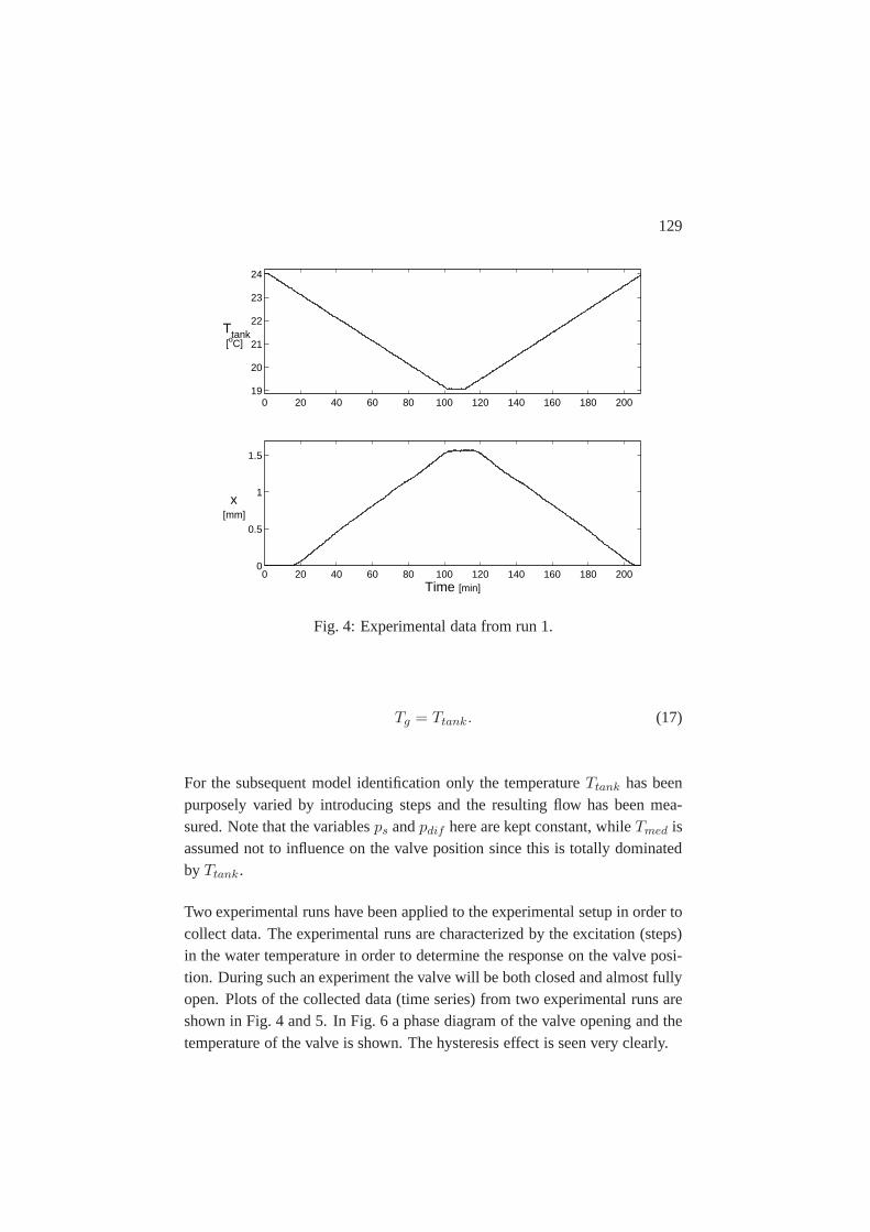
129
0 20 40 60 80 100 120 140 160 180 2000
0.5
1
1.5
x[mm]
Time [min]
0 20 40 60 80 100 120 140 160 180 20019
20
21
22
23
24
Ttank [oC]
Fig. 4: Experimental data from run 1.
Tg = Ttank. (17)
For the subsequent model identification only the temperatureTtank has beenpurposely varied by introducing steps and the resulting flow has been mea-sured. Note that the variablesps andpdif here are kept constant, whileTmed isassumed not to influence on the valve position since this is totally dominatedby Ttank.
Two experimental runs have been applied to the experimental setup in order tocollect data. The experimental runs are characterized by the excitation (steps)in the water temperature in order to determine the response on the valve posi-tion. During such an experiment the valve will be both closed and almost fullyopen. Plots of the collected data (time series) from two experimental runs areshown in Fig. 4 and 5. In Fig. 6 a phase diagram of the valve opening and thetemperature of the valve is shown. The hysteresis effect is seen very clearly.

130
0 20 40 60 80 100 1200
0.1
0.2
0.3
0.4
0.5
0.6
x[mm]
Time [min]
0 20 40 60 80 100 120
22
22.5
23
23.5
24
Ttank [oC]
Fig. 5: Experimental data from run 2.
22 22.5 23 23.5 240
0.1
0.2
0.3
0.4
0.5
0.6
0.7
x[mm]
Ttank [oC]
Fig. 6: Phase diagram of valve opening vs. valve temperature (run 2).

131
The uncertainties of the measured data used for model identification are listedin Tab. 1. The uncertainty in the flow and the various pressures are givenrelatively and the uncertainty of the temperatures are in absolute units.
Table 1: Measurement uncertaintiesVariable Symbol Uncertaintyσ Unit
flow q 0.015 · q kg/h
surrounding temperature Ttank 0.05 oC
differential pressure pdif 0.015 · pdif mbar
static pressure ps 0.015 · ps bar
5 RESULTS
The measured variables listed in Tab. 1 toghether with the model Eq. (15-16)has been applied and the unknown parameters have been estimated. Note thatthe pressure of the thermostat gas,∆pb(Tg), has been calculated using a higherorder polynomia for the relation between∆pb(Tg) andTg. Also, it should benoted that the valve positionx is calculated by a formula (table values) for therelation between the flow, differential pressure and the corresponding valveposition.
The parameters of the model that are known a priori, listed in Tab. 2. Theremaining parameters are unknown and have been estimated. First, the param-eters listed in Tab. 3 are found using data from a preliminary experiment wherethe temperature is constant, i.e. the hysteresis term±Fh is set to zero. Theseparameters are determined using the least squares criterion. Finally, the esti-mated parameters of the parameters for the hysteresis function are found usingthe ML method, keeping the remaining parameters of Tab. 2 and 3 constant.These estimated parameters of the hysteresis function are listed in Tab. 4.
As a first check the estimated model parameters are considered. Comparedto physical interpretation the estimates seem very reasonable indicating thatthe model formulation is realistic from a physical point of view. From an

132
Table 2: Known parameter valuesParameter Value Unit Description
Ab 1032 mm2 Area of BellowsCv 1.8 N/mm Valve springCi 13.7 N/mm Setting springCv 3.2 N/mm Bellows spring
Table 3: Estimated parameter values found by least squaresParameter Value Unit Description
As 2.45 mm2 Area of spindleAk 52.0 mm2 Area of coneKf 99.7 mm Flow spring
empirical point of view, a comparison between the measured and modelledoutput is shown in Fig. 7. It is seen that the model is able to predict the systemquite accurately.
The model residuals shows no systematic patterns, and this is supported bythe estimated autocorrelation function for the model residuals. The test inthe estimated autocorrelation function indicates a satisfactory model fit sinceno information is left in the model residuals, see e.g. (Holst et al. (1992)).As another comparision the estimated standard deviation of the residuals isσε = 2.4 · 10−3mm which corresponds to a relative uncertainty of 1%. Thisis less than the measurement uncertainty, listed in Tab. 1. As a comparison tothe play model the estimated variance on the prediction errors using the playmodel is larger by a factor 3, and also larger than the measurement uncertainty.
Table 4: Estimated parameters found by MLvariable estimate std.dev.
σ 6.41 0.589Fh,max 1.31 0.067pb,set 0.0776 0.892 · 10−3

133
20 40 60 80 100 1200
0.2
0.4
0.6
Tid [min]
x[mm]
measpredsim
20 40 60 80 100 120−0.01
0
0.01
εt[mm]
Tid [min]
0 2 4 6 8 10 12 14 16 18 20
0
0.5
1
lag
ρε
Fig. 7: Estimated model performance. Top: Measured, predicted and simulatedmodel output. Middle: Model residuals. Bottom: Estimated autocorrelationfunction for the residuals.
Thus, the proposed model is significantly better than the simple play model.Furthermore the model may be interpreted physically. Finally, a cross valida-tion study using the model estimated model on the independent experimentaldata from run 1 is shown in Fig. 8. It is seen that the model is still able topredict the system with high accuracy.
6 SUMMARY AND DISCUSSION
A grey box model of a thermostatic valve has been presented. The model isbased on physical interpretation and statistical methods has been used to es-timate and validate the model. The combination of physical knowledge andstatistical methods implies that the model can be interpreted physically andthat non-linear effects, such as hysteresis, can be handled effectively. Hystere-sis is a phenomena that makes the modeling of thermostatic valves difficult at

134
20 40 60 80 100 120 140 160 180 2000
0.5
1
1.5
Tid [min]
x[mm]
measpredsim
20 40 60 80 100 120 140 160 180 200
−0.01
0
0.01
εt[mm]
Tid [min]
0 2 4 6 8 10 12 14 16 18 20
0
0.5
1
lag
ρε
Fig. 8: Cross validation of the model. Top: Measured, predicted and simulatedmodel output. Middle: Model residuals. Bottom: Estimated autocorrelationfunction for the residuals
least if the approach is solely based on empirical data. To overcome this prob-lem an adaptive model for friction was applied to overcome for the hysteresiseffect. Using statistical methods it was shown that the model is able to describeempirical data with high accuracy. If the model should be applied for systemanalysis it might be necessary to model the heat dynamics of the thermostat aswell. However, the model for the valve position would probably still be valid.Since the Dahl model does not account for the static friction, a possibility isto use Bliman-Sorine models, in order to compensate for the lacking term Ols-son et al. (1997). The Bliman-Sorine models can be interpreted as two parallelDahl models, one fast and one slow. The fast has a larger (maximal frictionforce - steady state friction) than the slow one. Another aspect is to apply themodel for dynamic simulations, e.g. in simulaiton of building dynamics. Thiswould imply that the dynamics of the thermostat has to be considered as well.Preliminary results show that the model presented in this study is still usefuland adequate. The results of the dynamic model will be given in a subsequentpaper.

Paper F
MODELLING THE HEATDYNAMICS OF A BUILDING
USING STOCHASTICDIFFERENTIAL EQUATIONS
F135


137
ABSTRACT
This paper describes the continuous time modelling of the heat dynamics of abuilding. The considered building is a residential like test house divided intotwo test rooms with a water based central heating. Each test room is dividedinto thermal zones in order to describe both short and long term variations.Besides modelling the heat transfer between thermal zones, attention is puton modelling the heat input from radiators and solar radiation. The appliedmodelling procedure is based on collected building performance data and sta-tistical methods. The statistical methods are used in parameter estimation andmodel validation, while physical knowledge is used in forming the model struc-ture. The suggested lumped parameter model is thus based on thermodynam-ics and formulated as a system of stochastic differential equations. Due to thecontinuous time formulation the parameters of the model are directly physicalinterpretable. Finally, the prediction and simulation performance of the modelis illustrated.
Keywords: Stochastic differential equations, heat dynamics, parameter esti-mation, ML method.
1 INTRODUCTION
The use of models for the heat dynamics in a building is a perceptive and prac-ticable method to reduce the energy consumption and to improve the thermalcomfort. A model can serve as a useful tool in e.g. selecting insulation mate-rials, analyzing control strategies or in the design of a suitable heating system.Along with the varieties of applications, two different modelling proceduresmay be used. The traditional approach is to use knowledge of the physi-cal building characteristics and models of subprocesses and by those meansachieve a deterministic model. An alternative method is to use building perfor-mance data and statistical methods.
Various deterministic approaches are described in the literature, see e.g. Mitchell

138
and Beckman (1995), while the literature on statistical approaches is less. Astatistical approach,the grey box modelling method, is applied by Madsen andHolst (1995) in order to derive a total model for the heat dynamics of a build-ing with a single test room. The proposed model is formulated as a systemof stochastic differential equations and a Maximum Likelihood (ML) methodis used for estimation of the parameters in the continuous-time model, basedon discrete-time building performance data. As argued in Madsen and Holst(1995) there are in particular two main differences between the grey box mod-elling approach and the traditional deterministic approach. Firstly, while thetraditional approach uses knowledge about the physical characteristics only,the grey box model structure can be identified using both knowledge about thephysical characteristics of the building and information from building perfor-mance data. Secondly, while the traditional approach is kept in a deterministicframework, the grey box approach is kept in a stochastic framework. Herebystatistical methods can be applied in identifying a suitable parameterization.This is often a very difficult task using the traditional approach.
In this paper the grey box modelling method is applied. The attention is fo-cused on modelling the heat dynamics of the indoor air temperature in a res-idential like building when excited by various heat inputs, such as solar radi-ation and heat from radiators. The building considered is a low energy testbuilding from where building performance data from a planed experiment isused. The modelling task is extended compared to the model presented inMadsen and Holst (1995). It consists of modelling the heat dynamics in var-ious rooms of the test building, each differently affected by solar radiation.Furthermore, the power from the radiators is not known completely and hasto be modelled as well. As in Madsen and Holst (1995), the test house is notinhabited. The grey box modelling method, introduced in Section 2, is usedsince both information from the physics as well as information from the datacan be used in determining a reasonable parameterization. The test building isdescribed in Section 3 followed by a description of the building performancedata in Section 4. Using this information, a total model is presented in Section5. The model is formulated in continuous time, in terms of stochastic differen-tial equations. The continuous-time formulation ensures that the parameters ofthe model are directly physical interpretable, while the stochastic frame workpermits a description of the accuracy of the model. Statistical methods are

139
used to identify, estimate and validate the suggested model. The results arepresented in Section 6, and finally, a conclusion with discussion is given.
2 THE MODELLING APPROACH
In this section the applied modelling approach is introduced. The modellingprocedure may be described by a flowchart, sketched in Fig. 1. It consists ofthree stages: identification, estimation and validation. The loop continues untilan adequate parameterization of the model is found. In the following eachstage will be further discussed.
2.1 Identifying the model structure
The first step in the modelling procedure is to select a model structure. Both in-formation from physics and information from measurements are used to iden-tify a suitable model parameterization. The most important variables can berecognized, and insight of the most important dynamics can be achieved byexamination of measurements from the system. To model the impact from
IDENTIFICATIONof the model structure
NoYes
ESTIMATIONof unknown parameters
Use the model for simulation studies and system analysis
Is the model OK?
MODELVALIDATION
Information from physics
Information from dataInformation fromthe model validation
Fig. 1: The modelling procedure.

140
the assumingly most important variables, well known thermodynamic rela-tionships are used, and formulated in terms of a system of ordinary differentialequations:
dXt = f (Xt,Ut, θ, t) dt, (1)
whereXt ∈ Rnx is a vector of system states and the vectorUt ∈ R
nu containsthe known inputs. Finally,θ ∈ R
np is a vector of parameters. The lumpedmodel Eq. (1) provides a deterministic description of the evolution in time ofthe states of the system. It is obvious that any description of the form Eq.(1) gives only an approximation of the evolution of the true system. In orderto use Eq. (1) as the foundation for a description of the true variation of thestates a stochastic term is included in Eq. (1) leading to the following systemof stochastic differential equation:
dXt = f (Xt,Ut, θ, t) dt+ G(θ, t)dWt, (2)
whereWt is a standard Wiener process andG(θ, t) is a function describinghow the disturbance is entering the system. There are several reasons for in-troducing a noise term in Eq. (1), referring to Madsen and Holst (1996):
• Modelling approximations. The system described by Eq. (1) might bean approximation to the true system.
• Unrecognized and unmodelled inputs may affect the evolution of thestates.
• Measurements of the input are noise-corrupted.
For a discussion on the application of stochastic differential equations in physics,see e.g. Øksendal (1985).
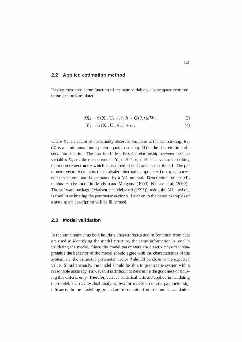
141
2.2 Applied estimation method
Having measured some function of the state variables, a state space represen-tation can be formulated:
dXt = f (Xt,Ut, θ, t) dt+ G(θ, t)dWt, (3)
Yt = h (Xt,Ut, θ, t) + et, (4)
whereYt is a vector of the actually observed variables at the test building. Eq.(3) is a continuous-time system equation and Eq. (4) is the discrete time ob-servation equation. The functionh describes the relationship between the statevariablesXt and the measurementsYt ∈ R
ny. et ∈ Rny is a vector describing
the measurement noise which is assumed to be Gaussian distributed. The pa-rameter vectorθ contains the equivalent thermal components i.e. capacitances,resistances etc., and is estimated by a ML method. Descriptions of the MLmethod can be found in (Madsen and Melgaard (1993); Nielsen et al. (2000)).The software package (Madsen and Melgaard (1993)), using the ML method,is used in estimating the parameter vectorθ. Later on in the paper examples ofa state space description will be illustrated.
2.3 Model validation
In the same manner as both building characteristics and information from dataare used in identifying the model structure, the same information is used invalidating the model. Since the model parameters are directly physical inter-pretable the behavior of the model should agree with the characteristics of thesystem, i.e. the estimated parameter vectorθ should be close to the expectedvalue. Simultaneously, the model should be able to predict the system with areasonable accuracy. However, it is difficult to determine the goodness of fit us-ing this criteria only. Therefor, various statistical tests are applied in validatingthe model, such as residual analysis, test for model order and parameter sig-nificance. In the modelling procedure information from the model validation

142
is a useful tool in improving the model performance. If the model validationindicates an inadequate model performance, information from the model vali-dation can indicate how to improve the model structure, as shown in Fig. 1, etcetera.
3 THE TEST BUILDING
This section yields a description of the test building and its heating system. Thepurpose is to emphasize on the most important building characteristics andthe influence from the heating system. This information is used in selectinga model structure for the heat dynamics in the test house. A more detaileddescription of the test building, the experimental design and the experimentcan be found in Hansen (1997).
The test building is located at the Technical University of Denmark (DTU),near Copenhagen, and was built around 1980. The termlow energy refers tothe nominal heat consumption, which is about 2.5 KW at−12 ◦C outside and20 ◦C inside, i.e. a nominal heat loss of∼ 78 W/◦C, Hansen (1996). The testbuilding is a single-storeyed building with a non-ventilated crawl space and a
NHU
EC
Control roomB Test roomAn
Test roomAs
12
Rad
iato
r
pc
Rad
iato
r
Fig. 2: A sketch of the test building and its interior.

143
roof space used as an office. The ground floor conforms a test area of 120 m2
and is divided into three rooms, as sketched in Fig. 2. The test rooms,As andAn, are used as test zones. The rooms are almost symmetrical and conformseach an area of 30 m2. Test roomAs has 3.6 m2 window area facing southwhile test roomAn has 1.9 m2 window area facing north. RoomB is 60 m2
and is used as a control zone. It contains some of the equipment for the exper-iment. All the windows in the control room are sheiled from solar radiation.The ceiling and the outer walls of the test building are light sandwich construc-tions based on a masonite beam insulated with 300 mm mineral wool, while thewalls separating the rooms are insulated with 95 mm mineral wool. The floorin each room are layer constructions which makes the building thermal heavyand the use of insulation makes the building extremely tight. A water basedcentral heating system is used for the heat supply. It consists of a heating unit,HU, placed in room B, and a radiator in each of the test rooms. The two radia-
Tn
Ts
Tb
Indoor Temperatures[◦C]
hours4003002001000
24
16
8
Tn
Ts
Outdoor temperatures[◦C]
hours4003002001000
14
7
0
Fig. 3: Measured temperatures from an experiment at the test building. Theindexes are as follows: s denotes south, n north and b the control room.

144
tors are identical with a nominal power of 395 W. The flow in each radiator iscontrolled by a thermostatic valve. An additional heat input is placed in roomAn, denoted EC. The EC-unit is remote controlled, i.e. a 0-5 V on/off signalcontrols an electrical on/off heat input of 0 or 150 W governed by a PRBS(Godfrey (1980)). The idea of the EC is to compensate for the sparse solarradiation on the northern side of the test building, Hansen (1996). Finally, thedata acquisition system (PC) performs measurements of pressure, flow, tem-perature, light sensors, and consists of converter equipment and a computer,which is used to store the measured data obtained from experiments.
4 THE DATA
In this section the dynamics of the most important variables will be discussed.The aim is to use this information in identifying the model structure. Theexperiment was carried out in the period 22/11-19/12 1996, and discussed inHansen (1997). Measurements from this experiment are used in the modellingprocedure. The following variables were measured at a frequency of 0.1 Hz:
Ti [◦C] indoor air temperatureTu [◦C] outdoor air temperatureI [W/m2] solar radiationTs [◦C] supply temperature to radiatorTr [◦C] return temperature from radiatorq [l/h] flow in radiator
The air temperatures were measured at several points in each of the threerooms, while the outdoor temperature and the solar radiation were measuredon the southern and northern side of the test building. Finally, the supply andreturn temperatures as well as the flow were measured at the radiator in eachtest room. Measurements of the air temperatures are plotted in Fig. 3. Consid-ering these time series, the dynamics of the air temperatures in the three rooms

145
In
Solar radiation, northern side[W/m2]
hours4003002001000
80
40
0
Is
Solar radiation, southern side[W/m2]
hours4003002001000
500
250
0
Fig. 4: Measurements of solar radiation.
are excited quite differently. This is as planed due to the experimental design,which has been performed to obtain the most informative data, see Hansen(1997). In order to excite the system, the experiment is started while the tem-perature in the building is low, i.e., the heating system has been shut down fora while in advance. The temperatures move towards a stationary temperaturein the test rooms, due to the different heat inputs. The stationary temperatureis determined by the set points of thermostatic valves, controlling the flow inthe radiators. In the control room,B, the temperatureTb is increasing slowly.The main heat input to the control room is probably the heat loss from theheating unit and the conductive heat transfer from the test rooms. Since thetest building is extremely tight, this explains the slow increment of the tem-perature. The solar radiation and the radiator flows, depicted in Fig. 4 and 5,respectively, affect the dynamics of the test room temperatures very differently.In the southern test room,As, the air temperatureTs is increasing rapidly whenthe solar radiation is high. Due to the thermostatic valve, the flow of water inthe radiatorqs is reduced each time the solar radiation is high. Hence, the radi-

146
qn
Flow in radiator, test roomAn [l/h]
hours4003002001000
70
35
0
qs
Flow in radiator, test roomAs [l/h]
hours4003002001000
70
35
0
Fig. 5: Measurements of radiator flow.
ator flow and the solar radiation are strongly correlated. On the northern side ofthe test building the measured solar radiationIn is severely limited comparedto the radiation on the southern side of the test building. Only a part of thediffuse solar radiation is measured on the northern side. The power from theEC-unit (150 W) is the main heat input for the northern test roomAn, and onlya very little flow, qn, is required to maintain a stationary temperature. Thus,the main heat inputs and hereby the excitation of the test rooms temperaturesare different. The main heat source in the northern test room is the EC-unitwhile the main heat source in the southern test room is the solar radiation andthe power from the radiator.

147
5 FORMULATION OF A MODEL
In this section the formulation of a linear model for the variations of the testroom air temperatures is proposed. The following items are considered impor-tant:
• The model should be able to describe all the dynamics of interest in theroom air temperatures, including the impact from the solar radiation andthe radiator power.
• The model should be formulated in continuous time in order to haveparameters which are physical interpretable.
• The model order should be as low as possible.
Besides the information from the measurements in Fig. 3-5, additionally in-formation from the measurements is obtained. In Fig. 6 the output from theEC-unit and the temperatureTn in the northern test room,An, is shown. Con-sidering the variations in the room air temperature, both a quick response afterthe input is shifted and a more persistent response are recognized. This indi-cates that at least two time constants are required for describing the short-termand the long-term variations of the room air temperatures in each test room, i.e.a second order model. In order to model both the short-term and the long-termvariations, the heat dynamics of the room air and of the thermal heavy con-structions are considered. This approached is described in Madsen and Holst(1995) and it is found useful if the short-term variations of the room air tem-perature are important, as for instance when controllers containing a feedbackfrom the room air temperature are considered. While the information from thedata indicates that at least a second order model is required, the attention isturned towards the test building. The goal is to obtain some equations describ-ing the heat dynamics of the room air and the thermal heavy constructions,which in this particular case is the floor. Hereby, each test room are regardedas two different thermal zones, the air and the floor. The heat equations foreach zone are formed by considering the heat transfer, i.e. conduction, con-vection and radiation, that is assumed to have greatest influence on the heat

148
ΦEC
Tn
Output from EC - temperature in northern test room
hours4003002001000
Fig. 6: The heat output from the EC-unit and the temperature in the northerntest room.
dynamics in the test building. As argued in Section 4, it is assumed that themost important heat transfer that influences on the room air temperature areheat input from solar radiation, the EC-unit, the radiators and conductive heattransfer through the walls and floor in each room, as sketched in Fig. 7. Sim-ilarly, the most important heat transfer that directly affects the temperature ofthe floor are assumed to be heat input from solar radiation and conductive heattransfer from the room air. Taking the model approximations into account,i.e. neglecting further heat transfer, the heat dynamics can be expressed as asystem of ordinary differential equations, see e.g. Ljung and Glad (1994):
d(Heat stored)dt
=∑
Power in−∑
Power out, (5)
⇒ CidTi
dt=∑
Φin −∑
Φout, (6)
whereC (J/K◦C) denotes heat capacity,T denotes temperature (◦C) andΦ (W)the heat transfer that is appraised to influence on the heat dynamics. To derivea parameterization forΦ, well known deterministic expressions for convective,conductive and radiate heat transfer are applied. The conductive heat transferthrough the walls and floor are modelled by a simple first order differential
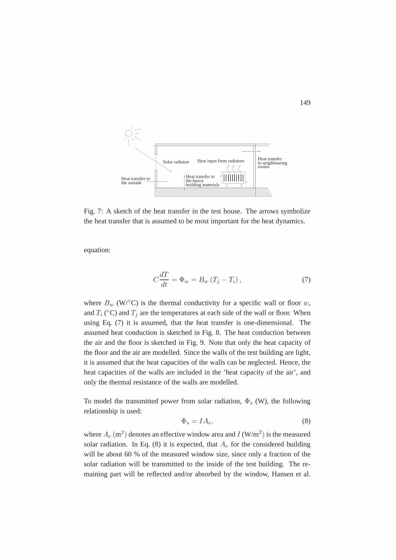
149
Heat transfer tothe heavybuilding materials
rooms
Heat transfer tothe outside
Solar radiaton Heat input from radiators Heat transferto neighbouring
Fig. 7: A sketch of the heat transfer in the test house. The arrows symbolizethe heat transfer that is assumed to be most important for the heat dynamics.
equation:
CdT
dt= Φw = Bw (Tj − Ti) , (7)
whereBw (W/◦C) is the thermal conductivity for a specific wall or floorw,andTi (◦C) andTj are the temperatures at each side of the wall or floor. Whenusing Eq. (7) it is assumed, that the heat transfer is one-dimensional. Theassumed heat conduction is sketched in Fig. 8. The heat conduction betweenthe air and the floor is sketched in Fig. 9. Note that only the heat capacity ofthe floor and the air are modelled. Since the walls of the test building are light,it is assumed that the heat capacities of the walls can be neglected. Hence, theheat capacities of the walls are included in the ’heat capacity of the air’, andonly the thermal resistance of the walls are modelled.
To model the transmitted power from solar radiation,Φs (W), the followingrelationship is used:
Φs = IAe, (8)
whereAe (m2) denotes an effective window area andI (W/m2) is the measuredsolar radiation. In Eq. (8) it is expected, thatAe for the considered buildingwill be about 60 % of the measured window size, since only a fraction of thesolar radiation will be transmitted to the inside of the test building. The re-maining part will be reflected and/or absorbed by the window, Hansen et al.

150
Bw = AwRw
TiTj
Ci
Fig. 8: Model approximations for the conductive heat transfer through a wall.
Ci
Ca
(air)
Ba = ARa
(floor)
Ta
Ti
Fig. 9: The conductive heat transfer between the air and the floor.
(1990). Furthermore, it is assumed, that both the air temperature and the floortemperature are affected by the solar radiator, i.e. a fractionp of the solar radi-ationΦs is transmitted directly to the floor while the remaining part,(1 − p),will directly heat the air. Hereby, the input from solar radiation is modelled as:
Φs,air = (1 − p)IAe Φs,floor = pIAe. (9)
Now, Eq. (5) can be used to describe the heat dynamics for the temperature ofthe air and floor in a single test room, respectively:
CidTi
dt=∑walls
Bw (Tj − Ti) +Ba (Ta − Ti) + (1 − p)Φs + Φr + ΦEC .
(10)
CadTa
dt=Ba (Ti − Ta) + pΦs. (11)

151
In Eq. (10) the power from the radiators is denotedΦr. The heat output fromthe EC-unit is known quite well, and is not modelled. In the following differentmodels forΦr will be suggested. A simple model, see e.g. Albrechtsen (1992),is given by:
Φr = cpρq(Tf − Tr), (12)
wherecp (W/K) is the specific heat capacity of the water in the radiator,ρ
(kg/m3) is the mass density of the water,q (m3/s) is the flow andTf andTr
(◦C) is the supply and return water temperature. Eq. (12) simply states, that thepower from the radiators is equal to the change in energy of the water, when itruns through the radiator. Another simple model is given by:
dQ
dt= cTd where Td =
Tf + Tr
2− Ti, (13)
wherec is a constant. Eq. (13) is reported to be useful in situations where theflow is not too varying, Benonysson (1991).If it is important to model the dynamics of the radiator as well, the followingfirst order equation can be used:
CrdTrad
dt= cpρq (Tf − Tr) −Br (Trad − T`)
n , (14)
whereTrad is the mean temperature of radiator surface andn is the radiatorexponent, Hansen (1997). When using Eq. (12) or (13) to model the radia-tor power each test room is modelled by two differential equations, as in Eq.(10-11). Using Eq. (14) implies three equations for each room. Thus, usingthe radiator model Eq. (12) or (13) a model for the heat dynamics of the testbuilding can be formulated:

152
Ci,sdTi,s
dt=Bu,s (Tu,s − Ti,s) +Bb (Tb − Ti,s) +Bn (Ti,n − Ti,s)
+Ba,s (Ta,s − Ti,s) + Φr,s +Ae,s (1 − ps) Is (15)
Ca,sdTa,s
dt=Ba,s (Ti,s − Ta,s) + psAe,sIs (16)
Ci,ndTi,n
dt=Bu,n (Tu,n − Ti,n) +Bb (Tb − Ti,n) +Bn (Ti,s − Ti,n) (17)
+Ba,n (Ta,n − Ti,n) + Φr,n + ΦEC +Ae,n (1 − pn) In (18)
Ca,ndTa,n
dt=Ba,n (Ti,n − Ta,n) + pnAe,nIn (19)
The parameters in Eq. (15-19) are specifized in the nomenclature. The systemof differential equations, Eq. (15-19), is obvious an approximation to the truesystem. According to the discussion in Section 2, the system is formulatedin terms of stochastic differential equations, yielding the linear state space de-scription:
dX = AXdt+ BUdt+ dW, (20)
Y = CX + DU + e. (21)
Eq. (15-19) written matrix form implies:
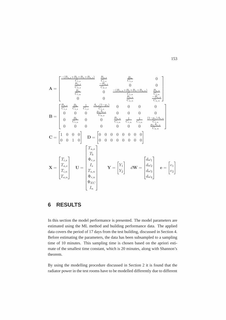
153
A =
−(Bu,s+Bb+Bn+Ba,s)Ci,s
Ba,s
Ci,s
BnCi,s
0Ba,s
Ca,s
−Ba,s
Ca,s0 0
BnCi,n
0 −(Bu,n+Bb+Bn+Ba,n)Ci,n
Ba,n
Ci,n
0 0 Ba,n
Ca,n
−Ba,n
Ca,n
B =
Bu,s
Ci,s
BbCi,s
1Ci,s
Ae,s(1−ps)Ci,s
0 0 0 0
0 0 0 psAe,s
Ca,s0 0 0 0
0 BbCi,n
0 0 Bu,n
Ci,n
1Ci,n
1Ci,n
(1−pn)Ae,n
Ci,n
0 0 0 0 0 0 0 pnAe,n
Ca,n
C =
[1 0 0 00 0 1 0
]D =
[0 0 0 0 0 0 0 00 0 0 0 0 0 0 0
]
X =
Ti,s
Ta,s
Ti,n
Ta,n
U =
Tu,s
Tb
Φr,s
IsTu,n
Φr,n
ΦEC
In
Y =
[Y1
Y2
]dW =
dω1
dω2
dω3
dω4
e =
[e1e2
]
6 RESULTS
In this section the model performance is presented. The model parameters areestimated using the ML method and building performance data. The applieddata covers the period of 17 days from the test building, discussed in Section 4.Before estimating the parameters, the data has been subsampled to a samplingtime of 10 minutes. This sampling time is chosen based on the apriori esti-mate of the smallest time constant, which is 20 minutes, along with Shannon’stheorem.
By using the modelling procedure discussed in Section 2 it is found that theradiator power in the test rooms have to be modelled differently due to different

154
excitation of the input variables. It is found that the diffuse solar radiation onthe northern side of the test building doesn’t influence the heat dynamics in thenorthern test room significantly. Contrary, the solar radiation on the southernside of the test building has a major impact on the heat dynamics in the southerntest room. It is found that only the air temperature is directly affected by solarradiation, i.e. the estimate of the fractionp is zero. Due to the fact that theradiators in the test rooms are controlled by thermostatic valves, the radiatorpower and the solar radiation are strongly correlated. This implies that Eq. (13)are suitable in modelling the radiator power in the northern test room while Eq.(12) and (14) are found adequate in the southern test room. The estimates andstandard deviations of the remaining model parameters of the model are shownin Tab. 1.
It should be noted that only the the thermal equivalent parameters of the modelEq. (15-19), which are found significant, are tabulated. The parameters valuesseems reasonable compared to their expected values. However, the estimatedvalues of the capacity of the indoor air are quite large. This can be explainedby the fact, that not only the capacity of the air is modelled, but also the heatcapacity of the interior in the test rooms and probably the inner part of thewalls, as also reported in Madsen and Holst (1996). From that point of view,
Symbol Estimate Unit Std. deviation
Bu, s 12.65 kJ/(Kh) 0.60
Bb 32.39 kJ/(Kh) 0.93
Bn 38.95 kJ/(Kh) 0.91
Ba, s 542.18 kJ/(Kh) 11.65
Bu, n 28.35 kJ/(Kh) 0.25
Ba, n 624.34 kJ/(Kh) 1.91
Ci, s 421.28 kJ/K 7.76
Ca, s 1531.85 kJ/K 67.46
Ci, n 810.19 kJ/K 15.75
Ca, n 3314.74 kJ/K 180.02
Ae,s 1.67 m2 0.02
Table 1: Parameter estimates of the model Eq. (15-19).

155
Northern room Southern room Unit
τair 25 42 min.
τfloor 23 26 hours
Table 2: Estimated time constants.
the estimates seem very reasonable and indicates in that the model parame-terization is suitable. Furthermore, the estimates of the time constants,τi arecalculated by the eigen-values,λi of the system matrixA, i.e. τi = −1/λi.The estimated time constants,τi, are listed in Tab. 2. These estimates are closeto their expected values. The heat dynamics of the air is fast compared to theslow heat dynamics of the floor, which was expected.
The model residuals have been analyzed to test if the residuals from the modelcan be accepted as being white noise. If this is the case, the model describesall the information given in the measurements. Test for white noise is appliedthrough estimation of the cumulated periodogram Eq. (22) and the autocorre-lation function Eq. (23):
C(vj) =∑j
i=1 I(vi)∑N/2i=1 I(vi)
whereI equals: (22)
I(vi) =1N
(N∑
t=1
ε(t)cos(2πvit)
)2
+1N
(N∑
t=1
(ε(t)sin(2πvit)
)2
,
ρ(k) =1
Nσ2ε
N−|k|∑t=1
(ε(t) − εµ)(ε(t + |k|) − εµ), (23)
whereεt denotes the prediction error or residual at timet. Hence, the residu-als are analyzed in both the frequency and time domain. The predicted statesand the equivalent measurements can not be distinguished in a graph, and istherefor not plotted. However, the statistical tests, Eq. (22) and Eq. (23) maybe shown visually. In Fig. 10 the residuals from each test room are compared

156
95 %
vj frequency0.50.40.30.20.10
1.0
0.75
0.5
0.25
0
95 %
lag20151051
0.15
-0.15-0.10-0.05
0.100.05
0
Fig. 10: Residual analysis of the prediction error. Top: Cumulated Peri-odogram for the residuals of the southern air temperature. Bottom: Autocorre-lation function for the residuals of the northern air temperature. In both cases,the residuals can be assumed to be white noise.
with the approximated 95% interval of significance. The statistical tests show,that the residuals of each test room can be regarded as white noise. This im-plies, that the model order is sufficient. Finally, a simulation performance ofthe model using the estimated parameters is shown in Fig. 11. Consideringthat the temperatures were measured with an accuracy of 0.25◦C and that themaximum difference between the simulated and measured temperatures, i.e.the simulation error, is 0.40◦C during the period of 17 days, the simulationperformance is considered excellent.

157
Ts[◦C]
hours4003002001000
24
16
8
Tn[◦C]
hours4003002001000
24
16
8
Fig. 11: Simulation performance during 17 days. Top: Simulation perfor-mance of the air temperature in the southern test room. Bottom: Simulationperformance of the air temperature in the northern test room.
7 CONCLUSION
In this paper a lumped parameter model describing the heat dynamics of aresidential like building has been proposed. The selected modelling methodwas the grey box modelling approach, i.e. the model was kept in a stochasticframework and the model structure was identified using both information frombuilding performance data as well as known thermal properties. The modelwas formulated as a system of stochastic differential equations and statisticmethods were applied for identifying, estimating and validating the model.
The heat dynamics in two test rooms were modelled. The two test rooms werefacing opposite directions, north and south, respectively, and were hereby verydifferently affected by the solar radiation. Each test room was divided into two

158
thermal zones in order to model both the short term and the long term varia-tions. Furthermore, submodels for the radiator power and the solar radiationwere presented. Finally, a linear state space model was formulated, in terms ofstochastic differential equations.
The model parameters were estimated using a ML method. Through statisticaltests and physical interpretation of the system, it was argued, that the modelgives a good description of the heat dynamics of the considered building. Dif-ferent models for the radiator power were found suitable in each test roomdue to the very different influence from the solar radiation on the northern andsouthern side of the building, respectively. Furthermore the radiator power,which was controlled by thermostatic valves, were strongly correlated with thesolar radiation and affected the choise of radiator models. The estimated pa-rameters seemed reasonable compared to the expected values of the equivalentthermal components. Furthermore, the residuals from the model could be ac-cepted as being white noise, which indicated that the model describes all thevariation in the data. Finally, it was shown that the model was able to simulatethe system with a very high accuracy.
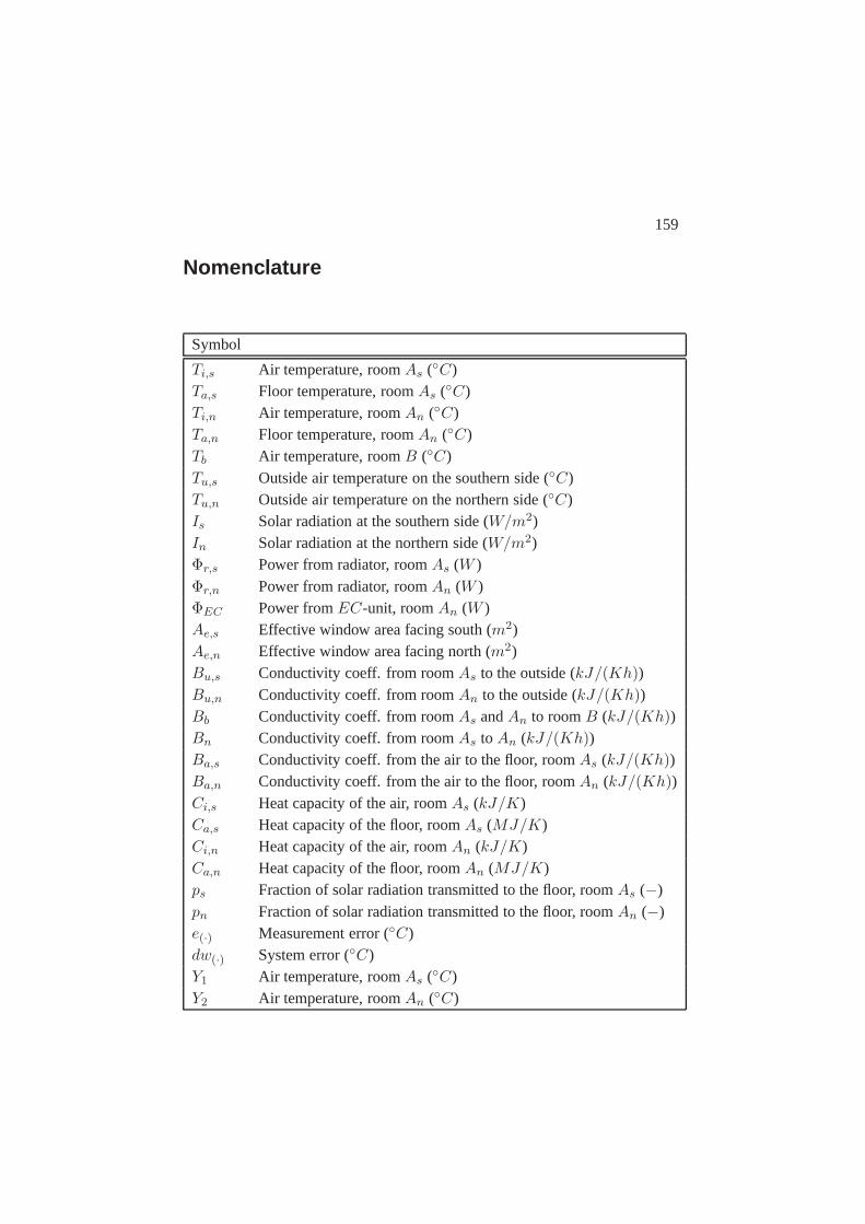
159
Nomenclature
Symbol
Ti,s Air temperature, roomAs (◦C)Ta,s Floor temperature, roomAs (◦C)Ti,n Air temperature, roomAn (◦C)Ta,n Floor temperature, roomAn (◦C)Tb Air temperature, roomB (◦C)Tu,s Outside air temperature on the southern side (◦C)Tu,n Outside air temperature on the northern side (◦C)Is Solar radiation at the southern side (W/m2)In Solar radiation at the northern side (W/m2)Φr,s Power from radiator, roomAs (W )Φr,n Power from radiator, roomAn (W )ΦEC Power fromEC-unit, roomAn (W )Ae,s Effective window area facing south (m2)Ae,n Effective window area facing north (m2)Bu,s Conductivity coeff. from roomAs to the outside (kJ/(Kh))Bu,n Conductivity coeff. from roomAn to the outside (kJ/(Kh))Bb Conductivity coeff. from roomAs andAn to roomB (kJ/(Kh))Bn Conductivity coeff. from roomAs toAn (kJ/(Kh))Ba,s Conductivity coeff. from the air to the floor, roomAs (kJ/(Kh))Ba,n Conductivity coeff. from the air to the floor, roomAn (kJ/(Kh))Ci,s Heat capacity of the air, roomAs (kJ/K)Ca,s Heat capacity of the floor, roomAs (MJ/K)Ci,n Heat capacity of the air, roomAn (kJ/K)Ca,n Heat capacity of the floor, roomAn (MJ/K)ps Fraction of solar radiation transmitted to the floor, roomAs (−)pn Fraction of solar radiation transmitted to the floor, roomAn (−)e(·) Measurement error (◦C)dw(·) System error (◦C)Y1 Air temperature, roomAs (◦C)Y2 Air temperature, roomAn (◦C)

160
Paper G
THE ERROR IN VARIABLES(EIV) REGRESSION
APPROACH AS A MEANSOF IDENTIFYING UNBIASED
PHYSICAL PARAMETERESTIMATES: APPLICATION
TO CHILLERPERFORMANCE
G
161


163
ABSTRACT
Classical regression analysis by the method of Ordinary Least Squares (OLS)considers errors to impact the dependent variable only, while it is implicitlyassumed that the independent or regressor variables are free of error. This as-sumption is frequently unrealistic, since measurement inaccuracies in the inde-pendent variables are sometimes very large. In such cases, model coefficientsidentified will be biased. While this may be an issue of secondary concernif the model is used for predictive purposes only, this would be problematicif the model coefficients are to be used for diagnostic purposes. A modelingapproach that can overcome this deficiency is the Error-In-Variable (EIV) re-gression approach that can provide unbiased parameter estimates even in thepresence of errors in the regressor variables (under the assumption that the er-rors are unbiased and normally distributed). This paper describes this method,and based on very precise chiller performance data measured in a laboratory,illustrates the benefit and advantage of the EIV method over the OLS method.An important finding of this study is that biased parameter estimates are verylikely to occur when OLS is used for identification even when well-maintainedfield instrumentation is used.
Keywords: Physical parameter estimation, Error In Variables Models, Ordi-nary Least Squares, Chiller Performance Modeling, Fault Detection and Diag-nosis.
1 INTRODUCTION
Regression analysis is widely used in the engineering science to describe em-pirical relationships between measured data. The most widely used methodof regression analysis is the Ordinary Least Squares (OLS) method that mini-mizes the sum of the squared residuals (see any statistical textbook, e.g. Draperand Smith (1981)). However, one of the basic assumptions in OLS, or in anyclassical regression analysis, is that the errors are present only in the depen-dent variables while the independent or regressor variables are free of error.

164
This assumption is frequently unrealistic, since sampling errors, measurementerrors, modeling errors etc. may imply random inaccuracies in the indepen-dent variables as well, (van Huffel and Vandewalle (1991)). A consequenceof neglecting the errors in the independent variables is that model parameterestimates obtained by OLS are biased; see e.g. Draper and Smith (1981). Apossible remedy that could remove this bias may be the use of Error in Vari-able (EIV) models, discussed in Draper and Smith (1981); J. and Fuller (1989);Fuller (1987); Casella and Berger (1990).
If the purpose of the model is purely predictive, then a model determined byOLS is probably as good as the EIV model for the mean predictive value, (vanHuffel and Vandewalle (1991)). However, the estimation of the associated un-certainty or confidence intervals or bands is an equally important issue. Sincethe prediction errors are calculated as the sum of the squared distances betweenthe dependent variable and the model predictions, the sum of squared residualswill be unrealistically small when using OLS. This will also imply that pre-diction intervals estimated by the OLS method will be misleadingly tighter,an issue of concern in certain types of applications, for example in fault de-tection using control chart techniques, (Box and Lucenco (1997)). How toestimate prediction confidence levels in such cases is treated in advanced sta-tistical textbooks, see e.g. Fuller (1987).
In many applications the accuracy of model parameters is important, especiallywhen the model parameters have be interpreted physically. An obvious exam-ple is the use of physical models for Fault Detection and Diagnosis (FDD) ofengineering systems. This type of model-based diagnosis has reached a cer-tain maturity in the engineering field, see e.g. Gertler (1998); Chen and Patton(1999) and is also being increasingly adopted to the FDD of HVAC&R com-ponents and systems, (Grimmelius et al. (1995); Han et al. (1999); Haves et al.(1996); Karki and Karjalainen (1999); Lee et al. (1996); Ng et al. (1997); Rossiand Braun (1997); Stylianou and Nikanpour (1996)).
The objective of this study is to evaluate the benefit in using the EIV modelapproach as compared to the OLS method. Specifically, we propose to performthe evaluation in the framework of a steady state chiller performance modelproposed by Gordon and Ng (1994, 1995) and later refined by Ng et al. (1997).

165
The Gordon-Ng model is derived from the laws of thermodynamics to whichrealistic approximations have been made in modeling the various heat transferphenomena occurring in actual chillers. The great benefit of the model is thatit is not only linear, but its formulation is such that the model parameters havea direct physical interpretation.
Comparison of both parameter identification approaches requires that we havethe "correct" physical parameters values to start with. We propose to over-come this difficulty by using published data by Ng et al. (1997) who madevery careful and meticulous performance measurements on a chiller in the lab,and also determined the physical parameters of the same chiller by direct mea-surement. Subsequently, we propose to add different noise levels to the chillerperformance data to mimic the larger uncertainties present in field measure-ments. Such data would allow us to investigate the extent to which OLS andEIV parameter estimates differ from the "correct" values as the noise level isincreased. Since the physical parameters are measured explicitly we can di-rectly evaluate whether or not the parameter estimates are biased. Aside fromcomparing the parameter estimates themselves, tests with different noise levelscan provide guidelines of how accurate the instrumentation for field monitoringshould be in order to obtain reasonable accurate physical parameter estimates.Furthermore, simulation studies with both the OLS and the EIV methods canprovide an indication of the extent to which sensor uncertainty influences thevariance of the parameter estimates.
The paper is organized as follows: The EIV method is described in section 2,followed by that of the Gordon-Ng model in section 3. In section 4 we describethe lab chiller data used for the comparison. Different methods to obtain theEIV estimates are discussed in section 5, and estimation and simulation resultsare presented in section 6. The final section provides a summary of the paper.
2 REGRESSION WITH EIV
Regression with errors in variables (EIV) is also known as the measurementerror model, see for example Draper and Smith (1981); Fuller (1987). The
166
model is a generalization of the simple linear regression of the form:
Yi = α+ βXi + εi, (1)
whereYi is the dependent variable(s),Xi is the regressor(s) or independentvariable(s),α andβ are the model parameters, andεi is the error term, hereassumed to be normally distributed with mean zero and varianceσ2
ε .
The main difference between OLS and EIV is that in the EIV model does notassume theXi to be known with full certainty. Instead the regressor variable istaken to be a random variable whose mean isXi. The general EIV model as-sumes that observed pairs(xi, yi) sampled are discrete realizations of randomvariables(Xi, Yi) whose means satisfy the linear relationship:
E[Yi] = α+ βE[Xi]. (2)
PosingE[Yi] = ηi andE[Xi] = ξi, the relationship given by Eq. (2) becomes:
ηi = α+ βξi, (3)
which is a linear relationship between the means of the random variables. Thevariablesηi andξi are sometimes called latent variables, a term that refers toquantities that cannot be directly measured. Latent variables may be not onlyimpossible to measure directly, but impossible to measure at all. If we areregressing onY onX, i.e. modeling as the response and as the regressor, wecan define the EIV model as:
Yi =α+ βxi + εi εi ∈ N(0, σ2ε ), (4)
Xi =ξi + δi δi ∈ N(0, σ2δ ), (5)

167
whereN(0, σ2) implies a normally distributed random number with mean 0and varianceσ2.
There are two different types of relationships that can be specified in the EIVmodel, one that specifies a linear functional relationship, and one describingthe structural linear relationship, following Casella and Berger (1990). Thelinear functional relationship is as described in Eq. (4). The parameters ofinterest areα andβ, and inference on these parameters is made using the jointdistribution of(Xi, Yi) conditional onξi.
For the structural model, the dependent variables are modeled asξi ∈ N(ξ, σ2ξ ).
As in the functional model, the parameters of interest areα andβ but infer-ence on these parameters is now made using the joint distribution of(Xi, Yi)unconditional onξi. For physical systems a functional relationship will oftenseem most appealing, and in this paper we will only consider models of thistype.
3 A PHYSICAL MODEL FOR CHILLER PERFOR-MANCE
In this section we will briefly describe the second-generation complete chillermodel proposed by Gordon and Ng (1994, 1995) and later extended Ng et al.(1997), which will henceforth be referred to as GN model. We shall applyboth the OLS and EIV method to obtain estimates of the physical parameters.The GN model is a simple, analytical, universal model for chiller performancebased on first principles of thermodynamics and linearized heat losses. Themodel predicts the dependent chillerCOP (defined as the ratio of chiller (orevaporator) thermal cooling capacityQch by the electrical powerE consumedby the chiller (or compressor) with specially chosen independent (and easilymeasurable) parameters such as the fluid (water or air) inlet temperature fromthe condenserTcdi, fluid temperature entering the evaporator (or the chilledwater return temperature from the building)Tchi, and the thermal cooling ca-pacity of the evaporator. The GN model is a three-parameter model which, forparameter identification, takes the following form:

168
(1
COP+ 1)Tchi
Tcdi− 1 = a1
Tchi
Qch+a2
(Tcdi − Tchi)TcdiQch
+a3(1/COP + 1)Qch
Tcdi,
(6)
where the temperatures are in absolute units, andQch andE are in consistentunits.
The parameters of the model given by Eq. (6), have physical meaning:
a1 = ∆S, the total internal entropy production in the chiller,a2 = Qleak, the heat losses (or gains) from (or in to) the chiller,a3 = R, the total heat exchanger thermal resistance(= 1
Ccd+ 1
Cch), whereC is
the effective thermal conductance of either the condensercd or the evaporatorch.
The authors point out thatQleak is typically an order of magnitude smallerthan the other terms. Though small, it is not negligible for accurate modeling.The authors suggest that it should be retained in the model if the other twoparameters being identified are to be used for chiller diagnostics.
Let us introduce:
x1 =Tchi
Qch, x2 =
(Tcdi − Tchi)TcdiQch
, x3 =(1/COP + 1)Qch
Tcdi, and (7)
y =(
1COP
+ 1)Tchi
Tcdi− 1. (8)
It is easily seen that the model given by Eq. (6) becomes:
y = a1x1 + a2x2 + a3x3. (9)
The model has been extended to apply to the case of variable condenser flowrate in Gordon et al. (2000). Though the final functional form is non-linear, theparameter estimation can be done using methods such as OLS and EIV.

169
4 DATA
The data in this study, taken from Ng et al. (1997), are from a semi-hermaticreciprocating chiller with a nominal cooling capacity of 10.5 kW. It consistsof 30 measurements of(Tchi, Tcdi, Qch, E) taken with high accuracy in a lab-oratory test loop. The units of these variables and their measurement accuracyare shown in Tab. 1. It is realistic to assume that the measurement errors of thedifferent variables share no common elemental source, i.e. that the errors areuncorrelated.
The data are plotted in Fig. 1 to provide the reader with a sense of the rangeof variation in the performance variables. Besides measuring the four perfor-mance variables, Ng et al. (1997) have also been able to separately measurethe individual physical parameters of the chiller, namely∆S,Qleak andR bymeans of intrusive component-level high-grade instrumentation. Based on the30 measurements, the mean and standard deviation of these measurements areshown in Tab. 2. The corresponding values obtained by OLS to the origi-
0 10 20 30280
282
284
286
288
290
292
K
Tchi
0 10 20 30296
298
300
302
304
306
308
310
K
Tcdi
0 10 20 309
10
11
12
13
14
15
kW
Qch
0 10 20 303.6
3.8
4
4.2
4.4
4.6
kW
E
Fig. 1: The data.

170
nal performance data are:R = 2.505KkW−1, ∆S = 5.55 10−3kWK−1,Qleak = 4.38kW . Note that these values are within the one standard deviation(except forQleak).
Table 1: Experimental uncertainty of the various performance variables for thechiller tested in a laboratory (taken from Ng et al., 1997).
Variable Tcdi Tchi Qch E
Uncertainty ±0.05 K ±0.05 K ±0.2 kW ±0.01 kW
Table 2: Mean value (E) and standard deviation (S) of the measurements of thephysical parameters in the Gordon-Ng model.
E[R] S[R] E[∆S] S[∆S] E[Qleak] S[Qleak]2.689 0.177 5.518 10−3 2.16 10−4 2.723 1.016
5 ESTIMATION BASED ON MOMENTS
In Section 2, the difference between the OLS and EIV methods was described.In this section we shall discuss how the model parameters can be estimated,suggest different ways of determining the influence of the measurement erroron the independent variables, and how to account for it.
In OLS estimation, the regression parameters are determined by:
βOLS = (XTX)−1XTY, (10)
whereX is a matrix of sizen × p, i.e. p independent variables each contain-ing n observations andY is a matrix of sizen × q, whereq is the numberof dependent variables. Again, it must be emphasized that using OLS (10),the independent variables,X, are assumed to be free of error. If the vari-ances of the measurement errors are known, the bias of the OLS estimator canbe removed and a consistent estimator, called Corrected Least Squares (CLS)can be derived, see e.g. van Huffel and Vandewalle (1991). The CLS correctsfor the extra source of error in an EIV model and can be considered to be a

171
method-of-moments. Assuming that the correlation between errors in the de-pendent variables and the errors in the independent variables are uncorrelated,the estimator becomes:
βCLS = (XTX − S2xx)−1(XTY − S2
xy), (11)
whereS2xx is ap× pmatrix with the covariance of the measurement errors and
S2xy is ap × 1 vector with the covariance between the regressor variables and
the dependent variable.
A simple conceptual explanation is that Eq. (11) performs on the estimatormatrix an effect essentially the opposite of what ridge regression, see any sta-tistical textbook, for example, Chatterjee (1991) does. While ridge regression’jiggles’ or randomly enhances the dispersion in the numerical values of thedependent variables in order to reduce the adverse effect of multi-collinearityon the estimated parameter bias, CLS tightens the variation in an attempt toreduce the effect of random error on the dependent variables.
We will compare the estimates obtained byβOLS andβCLS , respectively forthe GN model. The computation ofβOLS is straightforward, i.e. we can useEq. (10) directly. In order to determineβCLSwe will have to calculateS2
xx andS2
xy. This requires knowledge of the measurement errors, and assuming thatwe have this insight, one of three methods can be adopted:
1. Computation ofS2xx andS2
xy by propagation of errors.
2. Computation ofS2xx andS2
xy by applying stochastic calculus.
3. Computation ofS2xx andS2
xy by stochastic simulation.
The three methods will be discussed and compared with each other below.

172
5.1 Computation of and by propagation of errors
Consider a model (or a functionf ) such thatΦ = f(δ, γ, λ) and assume thatδ, γ andλ are measured with known uncertaintiesσ2
δ , σ2γ andσ2
λ respectively.Then the uncertaintyσ2
Φ in Φ can be approximated by the error propagationformula assuming the measurement errors of different variables to be uncorre-lated, i.e., assuming the covariance terms to be zero, see for example, Colemanand Steele (1999):
σ2Φ = σ2
δ (∂f
∂δ)2 + σ2
γ(∂f
∂γ)2 + σ2
λ(∂f
∂λ)2. (12)
Equation (12) can be used to compute the correction factors for the model.Since there are 3 independent variables and one dependent variable in the GNmodel, we have to compute a total of 9 correction factors, namely the elementsin the following:
S2xx =
S
2x1,x1 S2
x1,x2 S2x1,x3
S2x2,x1 S2
x2,x2 S2x2,x3
S2x3,x1 S2
x3,x2 S2x3,x3
, S2
xy =
S
2x1,y
S2x2,y
S2x2,y
, (13)
whereS2x1,x1 = σ2
x1 etc. To illustrate how the elements of the matrix in Eq.(13) are determined, we consider the GN model and the calculation ofS2
x1,x1,element (1,1) ofS2
xx which is the correction factor for the termx1x1. Recallfrom the GN model given by Eq. (6) that the regressor variablex1, was definedas:
x1 =Tchi
Qch.
Applying Eq. (12), the following correction factor is obtained:

173
S2x1,x1 = σ2
x1 = σ2T (
1Qch
)2 + σ2Q(Tchi
Q2ch
)2, (15)
whereσ2T andσ2
Q are the variance of the measurement error for the temperatureand the thermal load, respectively.
5.2 Computation of and by applying stochastic calculus
The calculation ofS2xx andS2
xy can also be done by comparing the expressionsof XTX andXTY for both noisy and noise-free variables and then applyingstochastic calculus. To illustrate how this is done, let us again consider the GNmodel and the calculation ofS2
x1,x1, the correction factor for the termx1x1.Since the variables in this expression are measured and thus contain error, itis to be realized that we are measuringTcdi = Tcdi + ε1, Tchi = Tchi + ε2,Qcd = Qcd + ε3 andE = E + ε4, whereεi denotes the measurement error forthe different variables, assumed normally distributed with mean 0 and varianceσ2
i . Thus, in the model the expression for thex1 variable can be written as:
x1 =(Tchi + ε2)(Qcd + ε3)
. (16)
For parameter estimation, the elementx1x1 (element 1,1 in ) becomes:
x1x1 =(
(Tchi + ε2)(Qcd + ε3)
)2
. (17)
The noise-free counterpart to Eq. (17) becomes:
x1x1 =(Tchi
Qcd
)2
. (18)
174
By comparing Eq. (17) where noise is included with the noise-free expressiongiven by Eq. (18) we can find the correction factorS2
x1,x1. We have:
x1x1 = x1x1 − S2x1,x1. (19)
The calculation ofS2x1,x1 can be done by applying stochastic calculus, namely
that in the computation we have assumed that the errors are independent withmean zero and variance equal to the square of the measurement error. In otherwords, for two sources of error, e.g.ε1 andε2 we have:
E[ε1] = 0, E[ε2] = 0, E[ε1ε2] = 0, E[ε1ε1] = σ21, E[ε2ε2] = σ2
2 , (20)
and all higher order terms (equal or higher than 3) are equal to zero. By doingso we find:
S2x1,x1 =
σ2QT
2chi + σ2
TQ2ch
Q2ch(Q2
ch + σ2Q)
, (21)
whereσ2T andσ2
Q are the variance of the measurement error for the temperatureand the thermal load, respectively. Although Eq. (21) may seem complicatedit can easily be computed with standard computer software such as MapleVor Mathematica. Furthermore, the method can provide answers to which mea-surement errors that will contribute the most to the correction factor and thusare most important to reduce. Finally, it should be noted that the expressiongiven by Eq. (21) is slightly different from the approximation found be themethod of propagation of errors, i.e. Eq. (15). However, the numerical valuesare almost identical, and in this study the influence of the approximation madeby propagation of errors has been found to be negligible.

175
5.3 Computation of and by applying stochastic simulation
Finally, an estimate of the correction factors may be found by stochastic (orMonte Carlo) simulation, also known as bootstrapping, see Davidson and Hink-ley (1997). The method may be useful if the data at hand is assumed noise-freeand one needs to investigate how increasing sensor error will affect the param-eter estimates. The following equation holds:
x1 = x1 − Sx1, (22)
wherex1 andx1 are noise-free and noisy values of the variablex1 respectively,andSx1is the measurement error.
The correction factor can be estimated by adding noise to the noise-free dataand then repeating this simulation to obtain a large data set (say, 1000 values)of noisy datax1 . The correction factor for each series is then found by:
S2x1,x1 = (x1 − x1)2. (23)
Finally, a consistent estimate of the correction factor may be obtained by aver-aging over the total number of simulation runs.
5.4 Comparison of the correction methods
The three different methods have both advantages and disadvantages, whichwill be discussed below.
The method of stochastic simulation is probably best if the data at hand is closeto being noise free and the purpose of the study is to investigate the affect ofneglecting measurement errors in the parameter estimation. The method is lessuseful if the data at hand is considered noisy and the purpose of the study isto obtain corrected and less biased parameter estimates. This is not an issue

176
for the two other methods, namely the propagation of errors and stochasticcalculus methods. These may be used to investigate the affect of neglectingmeasurement errors in the parameter estimation and to correct for parameterbias in noisy data.
The method of propagation may seem the most attractive from a practical view-point. Many standard programs exist which can provide estimates of the un-certainty due to errors in the variables and thus an estimate of the correctionfactors. However, a drawback is, as in this case, that if the same variables enterin the expression for the different regressors, the errors in the regressors arecorrelated and one has to be cautious in calculating the sign for the correctionfactor by propagation of errors. Say, we want to calculate the correction factor§2x1,x2 = Sx1Sx2 = σx1σx2. BothSx1 andSx2 can be calculated easily by thepropagation of errors, but will always be positive. Thus if the correction factorwere to be negative, special attention has to be given when using the method ofpropagation of errors. However, for many applications, the errors in the regres-sors are uncorrelated which reduces the problem to the calculation of only thediagonal elements inS2
xx, and, in such instances, the method by propagationof errors may be most suitable.
The problem with negative correction factors from using the method of prop-agation of errors is avoided when applying stochastic calculus. The methodgives the correct results but is not as well known, more tedious, and not asstraightforward as the propagation of errors method.
In general, we suggest applying the method using stochastic calculus when themeasurement errors in the regressors are correlated. If this is not the case, itmay be more attractive to use the method of propagation of errors. Finally,if the purpose is to get a rough estimate of the effect of measurement error onthe parameter estimates, the method of stochastic simulation may be the fastestand most attractive method.

177
6 EXAMPLE: THE GN MODEL
In this example, we will assume that the data presented in Section 4 are noisefree and illustrate the effect of neglecting measurement errors in the parameterestimation. The data has been measured with high accuracy in the lab andalthough there may be some measurement error we will neglect this in order toshow the principles of the EIV method.
Table 1 assembled the uncertainty in the four performance variables as dictatedby the instrumentation used. These accuracies are representative of the best,i.e. lowest uncertainties, one could hope to achieve in the laboratory. In thefield, the associated uncertainties are bound to be higher, and consequently,different levels of errors need to be introduced to this basic data set. We havedone so by generating normally distributed random numbers with different lev-els of standard deviation (to mimic precision error). Note that we have not in-troduced bias to the measurements themselves. Following Coleman and Steele(1999), one can assume the error which we propose to introduce effectivelyinclude both bias and precision measurement errors.
In an effort to be realistic in how we corrupt the data, we have chosen to main-tain the same magnitude of relative uncertainties of the four variables shown inTab. 1, and to use the same multiplier for all four variables. Hence a value of1.2 would imply that the uncertainties of all four variables have been increasedby 20% from those given in Tab. 1. For the purposes of the evaluation per-formed, we have taken the basic measured data and added normally distributednoise ranging from a magnitude from 0 to 2 (with step of 0.1). The selectionof the upper value of 2 is based on what we consider to be realistic uncertaintylevels to be found in well-maintained field instrumentation relating to chillers.
We have estimated the parameters for the data at different noise levels usingboth the OLS method and the EIV method. For the EIV parameter estimateswe have calculated the correction factors using all the three suggested methodsto ensure that all three methods yield equivalent results. In Fig. 2-4 the param-eter estimates in the GN model,∆S, Qleak andR, are shown when both theOLS and the EIV method are used for different magnitudes of noise added to

178
the data. The estimation for each parameter and noise level has been repeated1000 times using different noise sequences. The mean and corresponding 95%confidence intervals are shown in the plots. It is seen that as the noise levelincreases, the OLS estimates drift away from their true values. When the mag-nitude of the errors are greater than about 1.4 the true parameter values falloutside the 95% confidence level and may be regarded as being statisticallydifferent. Since a multiplier of 2.0 is representative of the uncertainty level tobe found even in well-maintained field instrumentation, it is clear that unbiasedparameter estimates are very likely to occur if OLS is used for identification.This is not the case for the EIV method. It is seen that the mean value of theparameter estimates are very close to the true values even when the magnitudeof error is as large as 2.0. Thus this example illustrates, that when magnitudeof the measurement error is known, consistent estimates can be obtained by theEIV method which avoids the biased estimates problem that plagues the OLSmethod.
The practical implication towards, say, chiller FDD work, is wthat physicalparameters estimated by the OLS method and used in a control chart, see e.g.Box and Lucenco (1997), setting to detect the onset of deviations or faultsin chiller performance, are likely to be biased and lead to mis-interpretationand false alarms. Parameters estimated by the EIV method are likely to yieldphysical parameters much more consistent with those determined by the chillermanufactures under careful in-house lab tests using high-grade sensors.
We have also investigated how the width of the uncertainty bands on the pa-rameter estimates (not to be confused with those of model prediction) of theOLS and EIV models in the figures above are affected by larger sample size,and whether the widths differ between both methods. We found that, as ex-pected, a larger sample size will lead to more accurate estimates and tighterparameter confidence bands, but that the width of the bands by both methodswere essentially similar.

179
0 0.2 0.4 0.6 0.8 1 1.2 1.4 1.6 1.8 25
6
7
8
9
10x 10
−3
∆ S
OLS − Magnitude of error
Mean95% limitsNoise free
0 0.2 0.4 0.6 0.8 1 1.2 1.4 1.6 1.8 21
2
3
4
5
6
7
8x 10
−3
∆ S
EIV − Magnitude of error
Mean95% limitsNoise free
Fig. 2: Comparison of OLS (top) and EIV (bottom) estimates of the entropy.
0 0.2 0.4 0.6 0.8 1 1.2 1.4 1.6 1.8 2−4
−2
0
2
4
6
Qle
ak
OLS − Magnitude of error
Mean95% limitsNoise free
0 0.2 0.4 0.6 0.8 1 1.2 1.4 1.6 1.8 20
2
4
6
8
10
12
14
Qle
ak
EIV − Magnitude of error
Mean95% limitsNoise free
Fig. 3: Comparison of OLS (top) and EIV (bottom) estimates of the heat losses.

180
0 0.2 0.4 0.6 0.8 1 1.2 1.4 1.6 1.8 21
1.5
2
2.5
3
R
OLS − Magnitude of error
Mean95% limitsNoise Free
0 0.2 0.4 0.6 0.8 1 1.2 1.4 1.6 1.8 21.5
2
2.5
3
3.5
4
R
EIV − Magnitude of error
Mean95% limitsNoise Free
Fig. 4: Comparison of OLS (top) and EIV (bottom) estimates of the heat ex-changer thermal resistance.

181
7 SUMMARY
The objective of this paper was to demonstrate that unbiased parameter esti-mates can be identified by the EIV regression approach when errors are presentin the regressor variables, while OLS estimation can lead to biased estimates.However, in order for the EIV method to yield fully unbiased estimates, thelevels or magnitude of the measurement errors, assumed to be random andnormally distributed only, should be fairy well known in advance. Otherwisethe method may suffer from the same type of problem which the OLS methoddoes, namely biased estimates. It is obvious that practically even if one maynot know the exact magnitude of such errors, even a realistic guess-estimatewould be better than using OLS, the degree of lack of bias being in propor-tion to how accurately one is able to estimate the measurement errors in theregressors.
The paper also discussed the need for such a procedure in the framework ofchiller FDD. If the purpose of the chiller model identified from actual perfor-mance data is to predict future chiller performance, model parameter bias isnot a critical issue. A model identified by OLS will probably predict the meanvalue of the response as well as that of an EIV model, though, the predictionuncertainty bands will be under-estimated leading to the occurrence of highfalse alarms during fault detection. However, when one wishes to interpret themodel parameters in terms of physical equipment health or performance, asprovided by say the Gordon-Ng chiller model, then model parameter bias as-sumes a new importance, and the EIV regression approach is clearly superiorto the OLS method. The evaluation of both identification methods is based onvery precise chiller performance data measured in a laboratory to which dif-ferent magnitudes of noise has been added to mimic field conditions. An im-portant finding of this study is that biased parameter estimates are very likelyto occur when OLS is used for identification even when well-maintained fieldinstrumentation is used.

182
NOMENCLATURE
C = thermal conductance of the heat exchangers of the chillerE = electric power consumed by the chillerQch = thermal cooling capacity of the chillerQleak = heat losses or gains from or into the chillerR = total heat exchanger thermal resistance∆S = total internal entropy production in the chillerS = standard deviationTcdi = fluid inlet temperature to the condenserTchi = fluid inlet temperature to the chiller or evaporatorX, x = regressor variable(s)Y, y = dependent variable(s)a1, a2, ..= model parametersn = number of observationsp = number of regressor variablesα, β = model parametersε, δ,Φ = errorσ2 = varianceξ = latent variable, or unobservable state variableη = latent variable, or unobservable state variableCOP = coefficient of performanceCLS = corrected least squaresEIV = error in variablesFDD = fault detection and diagnosisOLS = ordinary least squares

BIBLIOGRAPHY
Adunka, F. (1992). Heizkostenverteilung bei heikorpern mit start gedrosseltendurchflussen.HLH.
Albrechtsen, O. (1992). Central heating systems with water (in danish).
Andersen, K. K., Madsen, H., and Hansen, L. H. (2000). Modeling the heatdynamics of a building using stochastic differential equations.Energy andBuildings, 1(31), 13–24.
Antoulas, A. C. and Anderson, B. D. O. (1999). On the choise of inputs inidentification for robust control.Automatica, 35, 1009–1031.
Asprey, S. P. and Macchietto, S. (2000). Statistical tools for optimal dynamicmodel building.Computers and Chemical Engineering, 24, 1261–1267.
Bally, V. (1998). Construction of asymptotically optimal controls for controland game problems.Probability Theory Related Fields, 111, 453–467.
Benonysson, A. (1991). Dynamic modelling and operational optimization ofdistrict heating systems. ET, DTU.
Bianchi, C. and Cleur, E. M. (1996). Indirect estimation of stochastic differ-ential equation models: some computational experiments.ComputationalEconomics, 9, 257–274.
Bottin, S. and Chaté, H. (1998). Statistical analysis of the transition to turbu-lence in plane couette flow.The European Physical Journal B, 6, 143–155.
183

184
Bourdouxhe, J.-P., Grodent, M., and Lebrun, J. (1998). Reference guide for dy-namic models of hvac equipment. ASHRAE Research Project, Laboratoryof Thermodynamics, University of Liége.
Box, G. E. P. and Jenkins, G. M. (1970).Time Series Analysis, Forecastingand Control. Holden-Day, San Francisco.
Box, G. E. P. and Lucenco, A. (1997).Statistical Control by Monitoring andFeedback Adjustment. John Wiley & Sons, New York.
Brohlin, T. and Graebe, S. F. (1995). Issues in nonlinear stochastic grey-boxidentification. In Blanke and Söderström, editors,SYSID ’94, volume 3, pp.213–218. IFAC.
Cahlon, B., Schmidt, D., Shillor, M., and Zou, X. (1997). Analysis of thermo-stat models.Euro. Jnl of Applied Mathematics, 8, 437–457.
Casella, G. and Berger, R. L. (1990).Statistical Inference. Duxbury Press.
Chatterjee, S. (1991).Regression Analysis By Example Regression. John Wiley& Sons Ltd.
Chen, J. and Patton, R. J. (1999).Robust Model-Based Fault Detection forDynamic Systems. Kluwer Academic Publishers, Boston.
Cleveland, W. S. (1993).Visualizing data. Hobart Press.
Coleman, H. W. and Steele, W. G. (1999).Experimentation and UncertaintyAnalysis for Engineers. John Wiley & Sons.
Dahl, P. (1968). A solid friction model. Technical report, Aerospace Corp., ElSegundo, CA, USA.
Davidson, A. C. and Hinkley, D. V. (1997).Bootstrap Methods and their Ap-plications. Cambridge University Press.
Draper, N. and Smith, H. (1981).Applied Regression Analysis. John Wiley &Sons, New York, 2 edition.
Emery, A. F., Nenarokomov, A. V., and Fadale, T. D. (2000). Uncertainties inparameter estimation: the optimal experiment design.International Journalof Heat and Mass Transfer, 43, 3331–3339.

185
Forssell, U. and Ljung, L. (2000). Some results on optimal design.Automatica,36, 749–756.
Fox, R. W. and McDonald, A. T. (1985).Introduction to Fluid Mechanics.John Wiley & Sons.
Franck, G. and Rake, H. (1985). Identification of a large water-heated cross-flow heat exchanger with binary multifrequency signals.IFAC Identificationand System Parameter Estimation, pp. 1859–1864.
Freidlin, M. and Pfeiffer, R. (1998). A threshold estimation problem for pro-cesses with hysteresis.Statistics & Probability Letters, 36, 337–347.
Fuller, W. A. (1987). Measurement Error Models. John Wiley & Sons, NewYork.
Gard, T. C. (1988).Introduction to stochastic differential equations. MarcelDekker.
Gertler, J. J. (1998).Fault Detection and Diagnosis in Engineering Systems.Marcel Dekker Inc., New York.
Godfrey, K., editor (1993). Perturbation signals for system identification.Prentice Hall.
Godfrey, K. R. (1980). Correlation methods.Automatica, 16, 527–534.
Goodwin, G. C. (1982). Experiment design. InIFAC Identification and SystemParameter Estimation.
Goodwin, G. C. and Payne, R. L. (1977).Dynamic system identification: Ex-periment design and data analysis. Academic Press.
Gordon, J. M. and Ng, K. C. (1994). Thermodynamic modeling of reciprocat-ing chillers.Journal of Applied Physics, 75(6), 2769.
Gordon, J. M. and Ng, K. C. (1995). Predictive and diagnostic aspects of auniversal thermodynamic model for chillers.International Journal of HeatMass Transfer, 38(5), 807.

186
Gordon, J. M., Ng, K. C., Chua, H. T., and Lim, C. K. (2000). How varyingcondenser flow rate affects chiller performance: Thermodynamic modelingand experimental confirmation.Applied Thermal Eng., 20, 1149–1159.
Granger, C. and Lin, J. L. (1994). Using the mutual information coefficientto identify lags in nonlinear models.Journal of time series analysis, 15(4),371–384.
Grimmelius, H. T., Woud, J. K., and Been, G. (1995). On-line failure diagnosisfor compression refrigeration plants.International Journal of Refrigeration,18(1), 31–41.
Haerdle, W. (1990).Applied nonparametric regression. Cambridge UniversityPress.
Han, C. Y., Xiao, Y., and Ruther, C. J. (1999). Fault detection and diagnosis ofhvac systems.ASHRAE Transactions, 105.
Hansen, Kjerulf-Jensen, and Stampe, editors (1990).Varme- og klimateknik,Grundbog. DANVAK ApS.
Hansen, L. H. (1996). Dynamic analysis of a low energy test house and acentral heating system. technical report 20, IMM, DTU.
Hansen, L. H. (1997).Stochastic Modelling of Central Heating Systems. Ph.D.thesis, IMM, DTU.
Harremoes, P. and Madsen, H. (1999). Fiction and reality in the modellingworld-balance between simplicity and complexity, calibration and identifia-bility, verification and falsification.Wat. Sci. Tech., 39(9), 1–8.
Haves, P., Salsbury, T., and Wright, J. A. (1996). Condition monitoring inhvac subsystems using first principle models.ASHRAE Transactions, 102,519–527.
Hensen, J. (1996). Application of modelling and simulation to hvac systems.In 30th International Conference MOSIS.
Holst, J., Holst, U., Madsen, H., and Melgaard, H. (1992). Validation of greybox models. InIFAC Adaptive Systems in Control and Signal Processing,pp. 53–60, Grenoble, France.

187
Hurn, A. S. and Lindsay, K. A. (1997). Estimating the parameters of stochasticdifferential equations by monte carlo methods.Mathematics and computersin simulation, 43, 495–501.
Hurn, A. S. and Lindsay, K. A. (1999). Estimating the parameters of stochasticdifferential equations.Mathematics and computers in simulation, 48, 373–384.
J., B. P. and Fuller, W. A., editors (1989).Statistical Analysis of MeasurementError Models and Applications. AMS-IMS-SIAM. Proceedings of the JointSummer Research Conference.
Johansson, R. (1993).System modeling identification. Prentice Hall.
Jonsson, G. (1990).Parameter estimation in models of heat exchangers andgeothermal reservoirs. Ph.D. thesis, Department of Matematical Statistics,Lund Institute of Technology.
Jonsson, G. and Palsson, O. (1992). Use of empirical relations in the papame-ters of heat-exchanger models.The AMSE transaction, Journal of DynamicSystems, Measurements and Control, 30, 1193–1199.
Jonsson, G. and Palsson, O. (1994). An application of extended kalman filter-ing to heat exchanger models.The AMSE transaction, Journal of DynamicSystems, Measurements and Control, 116, 257–264.
Jonsson, G., Palsson, O., and Sejling, K. (1992). Modeling and parameter es-timation of heat exchangers - a statistical approach.The AMSE transaction,Journal of Dynamic Systems, Measurements and Control, 114, 673–679.
Jørgensen, S. B. and Hangos, K. M. (1995). Grey-box modeling for identifica-tion and control: An emerging discipline or an established technology? InBlanke and Söderström, editors,SYSID ’94, volume 3, pp. 231–236. IFAC.
Karki, S. H. and Karjalainen, S. (1999). Performance factors as a basis of prac-tical fault detection and diagnostic methods for air-handling units.ASHRAETransactions, 105.
Kayihan, A. (2000). Friction compensation for a process control valve.ControlEngineering Practice, 8, 799–812.

188
Khasminskii, R., Krylov, N., and Moshchuk, N. (1999). On the estimation ofparameters for linear stochastic differential equations.Probability TheoryRelated Fields, 113.
Kim, Y. T. (1999). Parameter estimation in infinite-dimensional stochasticdifferential equations.Statistics & Probability Letters, 45, 195–204.
Kinder, M. and Wiechert, W. (1996). Stochastic simulation of biotechnicalprocesses.Mathematics and Computers in Simulation, 42, 171–178.
Kloeden, P. E., Platen, E., and Schurz, H. (1997).Numerical Solution of SDEThrough Computer Experiments. Springer-Verlag. Berlin, 2 edition.
Lee, W. Y., Park, C., and Kelly, G. E. (1996). Fault detection in an air-handlingunit using residual and recursive parameter identification methods.ASHRAETransactions, 102, 528–539.
Li, T. H. (1998). Time-correlation analysis of nonstationary time series.Jour-nal of time series analysis, 19(1), 47–67.
Li, W. K. and Hui, Y. V. (1994). Robust residual cross correlation tests forlagged relations in time series.Journal of Statist. Comput. Simul., 49, 103–109.
Lindskog, P. and Ljung, L. (1995). Tools for semi-physical modeling. InBlanke and Söderström, editors,SYSID ’94, volume 3, pp. 237–242. IFAC.
Lindskog, P. and Ljung, L. (2000). Ensuring monotonic gain characteristics inestimated models by fuzzy model structures.Automatica, 36, 311–317.
Ljung, L. (1982). Model validation. InIFAC Identification and System Param-eter Estimation, pp. 73–75, Wahsington D.C., USA.
Ljung, L. and Glad, T. (1994).Modeling of dynamic systems. Prentice Hall.
Madsen, H. and Holst, J. (1995). Estimation of continuous-time models for theheat dynamics of a building.Energy and Buildings, 1(22), 67–79.
Madsen, H. and Holst, J. (1996). Modelling non-linear and non-stationary timeseries. IMM, DTU.
Madsen, H. and Melgaard, H. (1993).CTLSM - version 2.6. IMSOR, DTU.

189
McQuarrie, A., Shumway, R., and Tsai, C. L. (1997). The model selectioncriterion aicu.Statistics and Probability Letters, 34, 285–292.
Melgaard, H. (1994).Identification of physical models. Ph.D. thesis, IMM,DTU.
Mitchell, J. W. and Beckman, W. A., editors (1995).Building Simulation ’95,volume Fourth International Conference Proceedings, Madison, WisconsinU.S.A. International Building Performance Simulation Association.
Montgomery, D. C. (1991).Design and Analysis of Experiments. John Wiley& Sons Ltd., third edition.
Ng, K. C., Hua, H. T., Ong, W., Lee, S. S., and Gordon, J. M. (1997). Diag-nostics and optimisation of reciprocating chillers: Theory and experiment.Applied Thermal Engineering, 17(3), 263–276.
Nielsen, B. and Madsen, H. (1998). Identification of a linear continuous timestochastic model for the heat dynamics of a greenhouse.Journal of agric.Engng. Res., 71, 249–256.
Nielsen, H. and Madsen, H. (2001). A generalization of some classical timeseries tools.Computational Statistics & Data Analysis. accepted for publi-cation.
Nielsen, J. N., Madsen, H., and Young, P. C. (2000). Parameter estimation instochastic differential equations: an overview.Annual Reviews in Control,24, 83–94.
Norberg, R. (1995). Differential equations for moments of present values inlife insurance.Insurance: Mathematics and Economics, 17, 171–180.
Nowak, R. and Veen, B. V. (1993). Nonlinear system identification with pseu-dorandom multilevel excitation.IEEE International Conference on Acous-tics, Speech and Signal Processing, 4, 456–459.
Øksendal, B. (1985).Stochastic Differential Equations. Springer-Verlag.
Olsson, H., Aastrom, K. J., de Wit, C. C., Gafvert, M., and Lischinsky, P.(1997). Friction models and friction compensation. Technical report, LTH.

190
Palsson, O. P. (1993).Stochastic modeling, control and optimization of districtheating systems. Ph.D. thesis, IMSOR, DTU.
Paulsen, O. and Grundtoft, S. (1985). Dynamic testing of heating systems (indanish). Danish Institute of Technology.
Pazman, A. (1986).Foundations of optimal experimental design. KluwerAcademic Publishers.
Point, N., Wouwer, V., and Remy, M. (1996). Practical issues in distributedparameter estimation: gradient computation and optimal experiment design.Control Eng. Practice, 4(11), 1553–1562.
Ray, A. and Patankar, R. (1999). A stochastic model of fatigue crack propa-gation under variable-amplitude loading.Engineering Fracture Mechanics,62, 477–493.
Risken, H. (1996).The Fokker-Planck Equation. Springer, 2 edition.
Rossi, T. M. and Braun, J. E. (1997). A statistical rule-based fault detectionand diagnostic method for vapor compression air conditioners.Interna-tional Journal of Heating, Ventilating, Air-Conditioning and RefrigerationResearch, 3(1), 19–37.
Sadegh, P., Hansen, L. H., Madsen, H., and Holst, J. (1998). Input design forlinear dynamic systems using maxmin criteria.Journal of Information andOptimization Sciences, 19(2), 223–240.
Sejling, K. (1993). Modelling and prediction of load in district heating sys-tems. Ph.D. thesis, IMSOR, DTU.
Shao, J. (1993). Linear model selection by cross-validation.Journal of theAmerican Statistical Association, Theory and methods, 88(422), 486–494.
Sowa, J. (1998). Comparison of methods of including stochastic factors intodeterministic models of indoor air quality.Energy and Buildings, 27, 301–308.
Stylianou, M. and Nikanpour, D. (1996). Performance monitoring, fault de-tection, and diagnosis of reciprocating chillers.ASHRAE Transactions, 102,615–627.

191
Szilder, K., Lozowski, E. P., and Reuter, G. W. (1998). A stochastic model ofglobal atmospheric response to enchanced greenhouse warming with cloudfeedback.Atmospheric Research, 47-48, 475–489.
Tenno, R. and Uronen, P. (1995). State and parameter estimation for wastew-ater treatment processes using a stochastic model.Control Eng. Practice, 3,793–804.
Timmer, J. (2000). Parameter estimation in nonlinear stochastic differentialequations.Chaos, Solitons and Fractals, 11, 2571–2578.
Tong, H. (1990). Non-linear Time Series - A Dynamical System Approach.Clarendon Press Oxford.
Tulleken, H. (1992). Grey-box Modelling and Identification Topics. Ph.D.thesis, DELFT University of Technology.
Tulleken, H. (1993). Grey box modelling and identification using physicalknowledge and bayesian techniques.Automatica, 29(2), 285–308.
van Huffel, S. and Vandewalle, J. (1991).The Total Least Squares Problem -Computational Aspects and Analysis, volume 9. Frontiers in Applied Math-ematics.
Visintin, A. (1994).Differential models of hysteresis. Springer-Verlag.
Weyer, E., Szederkenyi, G., and Hangos, K. (2000). Grey box fault detectionof heat exchangers.Control Engineering Practice, 8, 121–131.
Wong, W. (1997). Frequency domain tests of multivariate gaussianity andlinearity. Journal of time series analysis, 18(2), 181–194.
Yarmolik, V. N. and Demidenko, S. N. (1988).Pseudorandom Sequences forRandom Testing. John Wiley & Sons Ltd.
Zarrop, M. B. (1979).Optimal experiment design for dynamic system identifi-cation. Springer-Verlag.
Zou, X., Jordan, J., and Shillor, M. (1999). A dynamical model for a thermo-stat.Journal of Engineering Mathematics, 36, 291–310.

192
Ph. D. theses from IMM
1. Larsen, Rasmus. (1994). Estimation of visual motion in image se-quences. xiv+ 143 pp.
2. Rygard, Jens Moberg. (1994). Design and optimization of flexiblemanufacturing systems. xiii+ 232 pp.
3. Lassen, Niels Christian Krieger. (1994). Automated determination ofcrystal orientations from electron backscattering patterns. xv+ 136 pp.
4. Melgaard, Henrik. (1994). Identification of physical models. xvii+246 pp.
5. Wang, Chunyan. (1994). Stochastic differential equations and a bio-logical system. xxii+ 153 pp.
6. Nielsen, Allan Aasbjerg. (1994). Analysis of regularly and irregularlysampled spatial, multivariate, and multi-temporal data. xxiv+ 213 pp.
7. Ersbøll, Annette Kjær. (1994). On the spatial and temporal correla-tions in experimentation with agricultural applications. xviii+ 345 pp.
8. Møller, Dorte. (1994). Methods for analysis and design of heteroge-neous telecommunication networks.Volume 1-2,xxxviii + 282 pp., 283-569 pp.
9. Jensen, Jens Christian. (1995). Teoretiske og eksperimentelle dy-namiske undersøgelser af jernbanekøretøjer. viii+ 174 pp.
10. Kuhlmann, Lionel. (1995).On automatic visual inspection of reflectivesurfaces.Volume 1,xviii + 220 pp., (Volume 2,vi + 54 pp., fortrolig).
11. Lazarides, Nikolaos. (1995). Nonlinearity in superconductivity andJosephson Junctions. iv+ 154 pp.
12. Rostgaard, Morten. (1995). Modelling, estimation and control of fastsampled dynamical systems. xiv+ 348 pp.
13. Schultz, Nette. (1995). Segmentation and classification of biologicalobjects. xiv+ 194 pp.

193
14. Jørgensen, Michael Finn.(1995).Nonlinear Hamiltonian systems. xiv+ 120 pp.
15. Balle, Susanne M.(1995). Distributed-memory matrix computations.iii + 101 pp.
16. Kohl, Niklas. (1995). Exact methods for time constrained routing andrelated scheduling problems. xviii+ 234 pp.
17. Rogon, Thomas.(1995). Porous media: Analysis, reconstruction andpercolation. xiv+ 165 pp.
18. Andersen, Allan Theodor. (1995). Modelling of packet traffic withmatrix analytic methods. xvi+ 242 pp.
19. Hesthaven, Jan.(1995).Numerical studies of unsteady coherent struc-tures and transport in two-dimensional flows.Risø-R-835(EN) 203 pp.
20. Slivsgaard, Eva Charlotte. (l995). On the interaction between wheelsand rails in railway dynamics. viii+ 196 pp.
21. Hartelius, Karsten. (1996). Analysis of irregularly distributed points.xvi + 260 pp.
22. Hansen, Anca Daniela.(1996). Predictive control and identification -Applications to steering dynamics. xviii+ 307 pp.
23. Sadegh, Payman.(1996).Experiment design and optimization in com-plex systems. xiv+ 162 pp.
24. Skands, Ulrik. (1996). Quantitative methods for the analysis of elec-tron microscope images. xvi+ 198 pp.
25. Bro-Nielsen, Morten. (1996). Medical image registration and surgerysimulation. xxvii+ 274 pp.
26. Bendtsen, Claus.(1996).Parallel numerical algorithms for the solutionof systems of ordinary differential equations. viii+ 79 pp.
27. Lauritsen, Morten Bach. (1997).Delta-domain predictive control andidentification for control. xxii+ 292 pp.

194
28. Bischoff, Svend.(1997). Modelling colliding-pulse mode-locked semi-conductor lasers. xxii+ 217 pp.
29. Arnbjerg-Nielsen, Karsten. (1997). Statistical analysis of urban hy-drology with special emphasis on rainfall modelling.Institut for Miljøteknik,DTU. xiv + 161 pp.
30. Jacobsen, Judith L.(1997). Dynamic modelling of processes in riversaffected by precipitation runoff. xix+ 213 pp.
31. Sommer, Helle Mølgaard.(1997).Variability in microbiological degra-dation experiments - Analysis and case study. xiv+ 211 pp.
32. Ma, Xin. (1997).Adaptive extremum control and wind turbine control.xix + 293 pp.
33. Rasmussen, Kim Ørskov.(1997). Nonlinear and stochastic dynamicsof coherent structures. x+ 215 pp.
34. Hansen, Lars Henrik. (1997).Stochastic modelling of central heatingsystems. xxii+ 301 pp.
35. Jørgensen, Claus. (1997). Driftsoptimering på kraftvarmesystemer.290 pp.

195
36. Stauning, Ole. (1997). Automatic validation of numerical solutions.viii + 116 pp.
37. Pedersen, Morten With. (1997).Optimization of recurrent neural net-works for time series modeling. x+ 322 pp.
38. Thorsen, Rune. (1997). Restoration of hand function in tetraplegicsusing myoelectrically controlled functional electrical stimulation of thecontrolling muscle. x+ 154 pp. + Appendix.
39. Rosholm, Anders. (1997). Statistical methods for segmentation andclassification of images. xvi+ 183 pp.
40. Petersen, Kim Tilgaard. (1997).Estimation of speech quality in telecom-munication systems. x+ 259 pp.
41. Jensen, Carsten Nordstrøm.(1997). Nonlinear systems with discreteand continuous elements.195 pp.
42. Hansen, Peter S.K.(1997). Signal subspace methods for speech en-hancement. x+ 226 pp.
43. Nielsen, Ole Møller. (1998). Wavelets in scientific computing. xiv+232 pp.
44. Kjems, Ulrik. (1998).Bayesian signal processing and interpretation ofbrain scans. iv+ 129 pp.
45. Hansen, Michael Pilegaard. (1998). Metaheuristics for multiple ob-jective combinatorial optimization. x+ 163 pp.
46. Riis, Søren Kamaric. (1998). Hidden markov models and neural net-works for speech recognition. x+ 223 pp.
47. Mørch, Niels Jacob Sand. (1998). A multivariate approach to func-tional neuro modeling. xvi+ 147 pp.
48. Frydendal, Ib. (1998.) Quality inspection of sugar beets using vision.iv + 97 pp. + app.
49. Lundin, Lars Kristian. (1998).Parallel computation of rotating flows.viii + 106 pp.

196
50. Borges, Pedro. (1998). Multicriteria planning and optimization. -Heuristic approaches. xiv+ 219 pp.
51. Nielsen, Jakob Birkedal. (1998). New developments in the theory ofwheel/rail contact mechanics. xviii+ 223 pp.
52. Fog, Torben. (1998). Condition monitoring and fault diagnosis in ma-rine diesel engines. xii+ 178 pp.
53. Knudsen, Ole.(1998). Industrial vision. xii+ 129 pp.
54. Andersen, Jens Strodl. (1998). Statistical analysis of biotests. - Ap-plied to complex polluted samples. xx+ 207 pp.
55. Philipsen, Peter Alshede. (1998). Reconstruction and restoration ofPET images. vi+ 132 pp.
56. Thygesen, Uffe Høgsbro.(1998).Robust performance and dissipationof stochastic control systems.185 pp.
57. Hintz-Madsen, Mads. (1998). A probabilistic framework for classifi-cation of dermatoscopic images. xi+ 153 pp.
58. Schramm-Nielsen, Karina.(1998).Environmental reference materialsmethods and case studies. xxvi+ 261 pp.
59. Skyggebjerg, Ole. (1999). Acquisition and analysis of complex dy-namic intra- and intercellular signaling events.83 pp.
60. Jensen, Kåre Jean.(1999). Signal processing for distribution networkmonitoring. xv+ 199 pp.
61. Folm-Hansen, Jørgen.(1999).On chromatic and geometrical calibra-tion. xiv+ 238 pp.
62. Larsen, Jesper. (1999). Parallelization of the vehicle routing problemwith time windows.xx+ 266 pp.
63. Clausen, Carl Balslev.(1999).Spatial solitons in quasi-phase matchedstruktures. vi+ (flere pag.)
64. Kvist, Trine. (1999).Statistical modelling of fish stocks. xiv+ 173 pp.

197
65. Andresen, Per Rønsholt. (1999). Surface-bounded growth modelingapplied to human mandibles. xxii+ 125 pp.
66. Sørensen, Per Settergren.(1999).Spatial distribution maps for benthiccommunities.
67. Andersen, Helle. (1999). Statistical models for standardized toxicitystudies. viii+ (flere pag.)
68. Andersen, Lars Nonboe. (1999). Signal processing in the dolphinsonar system. xii+ 214 pp.
69. Bechmann, Henrik. (1999). Modelling of wastewater systems. xviii+161 pp.
70. Nielsen, Henrik Aalborg. (1999).Parametric and non-parametric sys-tem modelling. xviii+ 209 pp.
71. Gramkow, Claus. (1999). 2D and 3D object measurement for controland quality assurance in the industry. xxvi+ 236 pp.
72. Nielsen, Jan Nygaard. (1999). Stochastic modelling of dynamic sys-tems. xvi+ 225 pp.
73. Larsen, Allan. (2000).The dynamic vehicle routing problem. xvi+ 185pp.
74. Halkjær, Søren. (2000).Elastic wave propagation in anisotropic inho-mogeneous materials. xiv+ 133 pp.
75. Larsen, Theis Leth. (2000). Phosphorus diffusion in float zone siliconcrystal growth. viii+ 119 pp.
76. Dirscherl, Kai. (2000). Online correction of scanning probe micro-scopes with pixel accuracy.146 pp.
77. Fisker, Rune. (2000).Making deformable template models operational.xx + 217 pp.
78. Hultberg, Tim Helge. (2000).Topics in computational linear optimiza-tion. xiv+ 194 pp.

198
79. Andersen, Klaus Kaae.(2001).Stochastic modelling of energy systems.xiv + 191 pp.
80. Thyregod, Peter. (2001).Modelling and monitoring in injection mold-ing. xvi+ 132 pp.
81. Schjødt-Eriksen, Jens.(2001).Arresting of collapse in inhomogeneousand ultrafast Kerr media.
82. Bennetsen, Jens Christian.(2000). Numerical simulation of turbulentairflow in livestock buildings. xi+ 205 pp + Appendix.
83. Højen-Sørensen, Pedro A.d.F.R.(2001). Approximating methods forintractable probabilistic models: - Applications in neuroscience. xi+104 pp + Appendix.
84. Nielsen, Torben Skov.(2001). On-line prediction and control in non-linear stochastic systems. xviii+ 242 pp.
85. Öjelund, Henrik. (2001).Multivariate calibration of chemical sensors.xviii + 184 pp.
86. Adeler, Pernille Thorup. (2001).Hemodynamic simulation of the heartusing a 2D model and MR data. xv+ 180 pp.
87. Nielsen, Finn Årup. (2001).Neuroinformatics in functional neuroimag-ing. 330 pp.
88. Kidmose, Preben.(2001).Blind separation of heavy tail signals. viii+136 pp.
89. Hilger, Klaus Baggesen.(2001). Exploratory analysis of multivariatedata. xxiv+ 186 pp.
90. Antonov, Anton. (2001).Object-oriented framework for large scale airpollution models.156 pp. + (flere pag).
91. Poulsen, Mikael Zebbelin. (2001). Practical analysis of DAEs.130pp.


![Hybrid Heat Pump Solutions for ... - DTU Research Database[14] [13] 3 DTU Mechanical Engineering, Technical University of Denmark DTU International Energy Conference11.9.2013. Advantages](https://static.fdocuments.us/doc/165x107/6122871c5d4e1e54b41a1367/hybrid-heat-pump-solutions-for-dtu-research-database-14-13-3-dtu-mechanical.jpg)


