...Please refer to following documents for more information on different cubes types and...
158
Transcript of ...Please refer to following documents for more information on different cubes types and...


Visit us at www.smarten.com 2
@ 2020, Smarten
Visit us at
Document Information
Document ID Smarten-Concept-Manual
Document Version Version 11.0
Product Version Version 5.1
Date 06-December-2020
Recipient NA
Author EMTPL
© Copyright Elegant MicroWeb Technologies Pvt. Ltd. 2020. All Rights Reserved.
Statement of Confidentiality, Disclaimer and Copyright
This document contains information that is proprietary and confidential to EMTPL, which shall not
be disclosed, transmitted, or duplicated, used in whole or in part for any purpose other than its
intended purpose. Any use or disclosure in whole or in part of this information without the express
written permission of EMTPL is prohibited.
Any other company and product names mentioned are used for identification purpose only, may be
trademarks of their respective owners and are duly acknowledged.
Disclaimer
This document is intended to support administrators, technology managers or developers using and implementing Smarten. The business needs of each organization will vary and this document is expected to provide guidelines and not rules for making any decisions related to Smarten. The overall performance of Smarten depends on many factors, including but not limited to hardware configuration and network throughput.

Visit us at www.smarten.com 3
@ 2020, Smarten
Visit us at
Contents
1 About this Document ............................................................................................................... 5 1.1 Scope and Organization of Topic Areas ..................................................................................... 5 1.2 Conventions Used ...................................................................................................................... 5
2 Introducing Smarten ................................................................................................................ 6
3 Designing the Data Model ........................................................................................................ 7 3.1 Cube Meta Data ......................................................................................................................... 7
3.1.1 Dimensions ...................................................................................................................... 8 3.1.2 Measures ......................................................................................................................... 8 3.1.3 Dimension Hierarchy ....................................................................................................... 9
3.2 Smarten Cache Cubes ............................................................................................................... 10 3.2.1 Cube Generation Process .............................................................................................. 10 3.2.2 Cube Update Process .................................................................................................... 11 3.2.4 Custom Cube Columns .................................................................................................. 16 3.2.5 Linked Cubes ................................................................................................................. 18 3.2.6 Supported Data Types ................................................................................................... 20
3.3 Smarten Real-Time Cubes ........................................................................................................ 21 3.4 Cube & Object Management .................................................................................................... 22
3.4.1 Matching Cube Criteria ................................................................................................. 22 3.4.2 Assigning Objects to another matching cube ............................................................... 23 3.4.3 Copy cube ...................................................................................................................... 23 3.4.4 Renaming the Cubes ..................................................................................................... 23 3.4.5 Renaming the Objects ................................................................................................... 23 3.4.6 Deleting the Cube without deleting dependent Objects .............................................. 23
3.5 Supported Features for Different Cubes .................................................................................. 24 3.5.1 Cube Management Functions ..................................................................................... 24 3.5.2 Analytic Functions ....................................................................................................... 25
4 Analytic Functions ................................................................................................................. 29 4.1 Slice & Dice ............................................................................................................................... 29 4.2 Drill down and Drill up.............................................................................................................. 29
4.2.1 Drill down ...................................................................................................................... 29 4.2.2 Drill up ........................................................................................................................... 30
4.3 Drill Through ............................................................................................................................. 31 4.4 Global Variables ....................................................................................................................... 34 4.5 Show only Summary data ......................................................................................................... 37 4.6 Sort. .......................................................................................................................................... 38
4.6.1 Simple Sort .................................................................................................................... 38 4.6.2 Advance Sort ................................................................................................................. 39 4.6.3 Custom Sort ................................................................................................................... 40
4.7 Group & Ungroup ..................................................................................................................... 41 4.8 Spotlighter ................................................................................................................................ 42 4.9 Data Value / Display Value mapping ........................................................................................ 45 4.10 UDDC & UDHC ........................................................................................................................ 46
4.10.1 Custom Measure (UDDC) ............................................................................................ 46 4.10.2 Custom Dimension Value (UDHC) ............................................................................... 47 4.10.3 Cell referencing in UDDC & UDHC ............................................................................... 49 4.10.4 Functions & Expressions ............................................................................................. 57
4.11 Data Operations ..................................................................................................................... 65 4.12 Summary Operations ............................................................................................................. 94 4.13 Trend Line ............................................................................................................................. 113
4.13.1 Linear Trend line ....................................................................................................... 114 4.13.2 Logarithmic Trend line .............................................................................................. 115 4.13.3 Polynomial Trend line ............................................................................................... 116 4.13.4 Power Trend line ....................................................................................................... 117

Visit us at www.smarten.com 4
@ 2020, Smarten
Visit us at
4.13.5 Exponential Trend line .............................................................................................. 118 4.13.6 Moving Average Trend line ....................................................................................... 119
4.14 Subview ................................................................................................................................ 120 4.15 What-if Analysis.................................................................................................................... 122 4.16 Master-Detail view in Tabular report ................................................................................... 125
5 Filters and Expressions ......................................................................................................... 127 5.1 Time Series (absolute, relative, range comparisons) ............................................................. 130
5.1.1 Absolute Time Series ................................................................................................... 131 5.1.2 Relative Time Series .................................................................................................... 132 5.1.3 Range Time Series ....................................................................................................... 139
5.2 Advanced Filter ...................................................................................................................... 140 5.3 Retrieval Parameters .............................................................................................................. 144 5.4 Global Variables ..................................................................................................................... 145 5.5 Rank ........................................................................................................................................ 147
5.5.1 Simple Rank ................................................................................................................. 147 5.5.2 Band Rank ................................................................................................................... 150
6 KPI…. ................................................................................................................................... 152 6.1 KPI elements & conventions .................................................................................................. 152
6.1.1 KPI Expressions ............................................................................................................ 153
7 Social BI .............................................................................................................................. 154
8 Access Rights & Security ...................................................................................................... 155 8.1 Column-based Access Rights (Column Access Permission) .................................................... 155 8.2 Dimension Value–based Access Rights (Data Access Permissions) ....................................... 156
9 Delivery & Publishing Agent ................................................................................................. 157
10 Product and Support Information ....................................................................................... 158

Visit us at www.smarten.com 5
@ 2020, Smarten
Visit us at
1 About this Document
This manual explains the concepts required to use the features in Smarten Augmented Analytics. Users with no prior experience with Augmented Analytics software can refer to this guide to learn and understand the concepts of Augmented Analytics in Smarten. Users who have experience with other BI tools can refer to this guide to map the Augmented Analytics functions to the Smarten features and understand the concepts from a logical angle.
1.1 Scope and Organization of Topic Areas
Chapter 2 Introducing Smarten
Chapter 3 Designing the Data Model
Chapter 4 Analytic Functions
Chapter 5 Filters & Expressions
Chapter 6 KPI
Chapter 7 Social BI
Chapter 8 Access Rights & Security
Chapter 9 Delivery & Publishing Agent
Chapter 10 Product and Support Information
1.2 Conventions Used
This manual uses typographical conventions in the text to help you distinguish between the names of files, instructions, and other important notes that are relevant during installation. For example:
Important notes are indicated in a different font colour as shown in the example below.
Note:
Apart from the data types listed above, other data types that are supported by a specific
database connection driver can also be supported by Smarten cubes.
References to documents are highlighted as below:
Reference: Concept Manual > Designing the Data Model > Cube Generation Process-Extraction
from CSV or flat files

Visit us at www.smarten.com 6
@ 2020, Smarten
Visit us at
2 Introducing Smarten
Augmented Analytics is a set of enterprise scale applications for gathering, indexing, storing, and analyzing data from various data sources and applications. It converts data into intelligent information, leading to a smarter and agile decision-making process. The integrated set of comprehensive features and functions in Smarten Augmented Analytics delivers actionable information to end users through dashboards, KPI, crosstab, graphs, GeoMap, and tabular.
HIGHER LEVEL ARCHITECTURE—SMARTEN
Using Smarten, users can access and analyze multidimensional data from multiple data sources such as RDBMS, text / csv files, and MDX data sources, using both real-time and cache cube architecture. Easy-to-use tools, such as dashboards, crosstab, graphs, GeoMap, tabular, KPI, alerts, and integrated delivery & publishing agent, are built on a “zero-footprint” browser–based Smarten user interface and can be accessed through the supported browsers on desktops, laptops, tablets, and smartphones. Smarten supports unique Managed Memory Computing that lets you choose data which will be used in-memory processing. Please refer to technical documents related to Managed Memory Computing for more details.

Visit us at www.smarten.com 7
@ 2020, Smarten
Visit us at
3 Designing the Data Model
This chapter details the basics of extracting data from different data sources, designing multidimensional objects called cubes, and preparing your data for crosstab, graphs, GeoMap, KPI, tabular, and dashboards. Smarten supports both real-time and cache cube architecture. There is also an option for aggregation in cache cubes, and user can choose if user wants to perform aggregation for cache cubes at cube level or not. Cache cubes will store indexed, pre-aggregated data along with metadata in the cubes. MDX and Real-time cubes will store only metadata information and will not store any data in the cubes. Please refer to following documents for more information on different cubes types and architecture.
Reference: Smarten-Working with Real time Cubes
Reference: Smarten-Working with SSAS MDX Cubes
Reference: Impact-of-Cube-Design-on-Performance > Cube type selection recommendations
3.1 Cube Meta Data
Smarten’s data extraction and cube management feature connects to the data sources to retrieve and transform the data based on logical rules and then loads that onto multidimensional cubes. The cubes in Smarten are the main source of the data extracted from various data sources. They are indexed with multidimensional data structure and optimized for high performance, high speed, high-volume queries, and analysis needs for quick and uniform response times. The following sections explain the underlining concepts of cube structure, such as dimensions, measures, time series, dimension hierarchy, and linked cubes.

Visit us at www.smarten.com 8
@ 2020, Smarten
Visit us at
A DIMENSIONAL MODEL OF A BUSINESS THAT HAS TIME, PRODUCT, AND REGION DIMENSIONS
3.1.1 Dimensions
Dimensions are the axes of a cube, representing x, y, and z coordinates. Aggregation of data with respect to more than one dimension is called multidimensional data. In the above figure, time, product category, and region are three dimensions of sales.
3.1.2 Measures
A measure is the scale or quantity of a dimension. In the above figure, measure is denoted by the numeric sales quantity in different colours.

Visit us at www.smarten.com 9
@ 2020, Smarten
Visit us at
3.1.3 Dimension Hierarchy
The dimension hierarchy refers to the hierarchical levels of data within a dimension map. Dimension maps can be defined at the cube level and enable automatic drill down and drill up to users. Dimension mapping means assigning the cube dimensions in terms of hierarchical levels. In the following illustration, the dimension city is mapped under the dimension state.
DIMENSION HIERARCHY SHOWING RELATIONSHIP BETWEEN STATE AND THEIR RESPECTIVE CITIES
Visit us at www.smarten.com 10
@ 2020, Smarten
Visit us at
DIMENSION HIERARCHY SHOWING MULTI-CHILDREN RELATIONSHIP BETWEEN PRODUCT CATEGORY, SKU, AND BRANDS
3.2 Smarten Cache Cubes
3.2.1 Cube Generation Process
Smarten allows you to extract data from various transactional, historical, and reference data sources (e.g., CSV, a flat file, databases, and/or any other data source used for creating the cube), for example, ERP or CRM database, or monthly sales data as a flat file export from your ecommerce application and form cubes. Cube extraction can be categorised broadly into two methods.
By Brand
By SKU

Visit us at www.smarten.com 11
@ 2020, Smarten
Visit us at
3.2.1.1 Extraction from Database
Typical steps for extraction from a database involves the following:
Configuration of a database profile using JDBC/ODBC driver
Connection with a database
Select Aggregation or No Aggregation option
Design SQL statement in two ways: o Graphical query designer o SQL query in editor
Meta data definition for cube by defining and mapping data source columns and cube dimension and measure columns
Define dimension map hierarchy
3.2.1.2 Extraction from CSV or flat files
CSV—Comma-separated values (also known as comma-separated variable) file format is a file type that stores tabular data. Typical steps for extraction from CSV files involve the following:
Locating CSV file and configuration of CSV data source profile
Identify row and column separators in CSV file
Identify field level parameters, such as data type, precision, length, scale, and format
Meta data definition for cube by defining and mapping CSV data source columns and cube dimension and measure columns
Define dimension map hierarchy
3.2.2 Cube Update Process
Once the cube is generated, the cube update process is used to append new data or refresh the cube with the most up-to-date data. It runs the predefined extraction query on data sources defined earlier and updates the cube according to the parameters selected.
3.2.2.1 Through Automatic Scheduler
For managing recency of the data used for multidimensional analysis, a cube should be regularly updated. The cube can be scheduled to regularly pull data from different data sources to update data at a given date/time. This is especially useful when the user knows exactly at what frequency the source data changes or when a particular type of data should be updated. The scheduling of cube updates can be monthly, weekly, daily, hourly, or on a “as and when required” basis for some specific occurrence based on the business needs and time required to update the cube.

Visit us at www.smarten.com 12
@ 2020, Smarten
Visit us at
Examples: Scheduler Frequency Description
One time Scheduler process is performed only one time on a specified date
Daily Scheduler process is performed daily
At every “n” hours Scheduler process is performed at every “n” number of hours. Ex: Every 2 hours
Weekly Scheduler process is performed on a specific day of a week. Ex: Every Wednesday of the week
Monthly Scheduler process is performed on a specific date of the month. Ex: Every 20th of the month
Yearly Scheduler process is performed yearly on a specified date and month of the year. Ex: Every 15 June
Start time Scheduler process is to be performed at a specific time; this can be achieved by setting the Start time in concurrence with One Time, Daily, Weekly, Monthly, or Yearly options. Ex: Schedule on 5 hours and 30 minutes daily
Term Scheduler process is to be performed for a specific term; it is a period in which the scheduler is activated. Ex: From 1 Aug 2014 to 31 Dec 2014
Reoccurrence Scheduler process is to be performed for some specific occurrence; it is used to end the scheduler process after some specific occurrence. Ex: End after 5 occurrences; it will end the scheduler process after 5 occurrences
Schedule On Scheduler Frequency
One time on 1 January 2014 at 1 a.m.
One time: 1 January 2014 Start time: 1 hour 0 minute
Every night at midnight Daily Start time: 0 hour 0 minute
Every Monday at 5 a.m. Weekly: Monday Start time: 5 hour 0 minute
3.2.2.2 Through Manual Process
This option helps the user to manually update a cube on an “as and when required” basis.
3.2.2.3 Types of Cube Updates—From scratch or incremental
3.2.2.3.1 From scratch update
When updating a cube from scratch, the cube is rewritten with all the records from the data source.

Visit us at www.smarten.com 13
@ 2020, Smarten
Visit us at
UPDATE FROM SCRATCH
3.2.2.3.2 Incremental update
With an incremental update, only the extracted data from the source is appended to the cube.
INCREMENTAL UPDATE
User can update cube with incremental option. In incremental option, system retrieves data from
data source and appends only new data into the cube. Smarten supports two options for
incremental update, one is, append all rows retrieved from data source and another is, append
new rows identified based on unique ID column.
For example, if you have selected the ‘ID’ column as a unique column from a cube and the highest
value in that column is ‘250’ in the cube. When you update the cube, the system retrieves only those

Visit us at www.smarten.com 14
@ 2020, Smarten
Visit us at
records that have value greater than ‘250’ in the ‘ID’ column and appends that data to the cube.
Same way, if you have selected the ‘Date’ column as a unique column from a cube and the highest
value in that column is ’10-10-2020’ in the cube, When you update the cube, the system retrieves
only those records that have value greater than ’10-10-2020’ in the ‘Date’ column and appends that
data to the cube.
3.2.3 Time Dimensions
Cubes usually need a time dimension for the time period–related queries that look at the periods—weeks, months, or years. Time dimension is a descriptive attribute about the date/time stamp field in the cube, for example, day of a week, a month, a quarter, a year, etc. Using time dimension, the hierarchical levels for the drill-down path is Year > Half Year > Quarter > Month > Week > Day > Hour > Minute > Seconds. The time dimension for a company can be based on either a calendar or a financial year.
3.2.3.1 Time Dimension Hierarchy
Time dimension hierarchy can be used to drill down from a summarized data of a year to a data up to a second level. As shown in the following example, users can drill down from a year up to a second level using time dimension hierarchy. It is possible for time dimension to be based on both a calendar year and a financial year.
THE TIME DIMENSION HIERARCHY
Note:
The calendar year starts from 1 January

Visit us at www.smarten.com 15
@ 2020, Smarten
Visit us at
3.2.3.2 Time dimension based on a calendar year
A calendar year starts on 1 January and ends on 31 December of each year. For any calendar year, the time dimension hierarchy would be as follows:
TIME DIMENSION HIERARCHY BASED ON A CALENDAR YEAR
3.2.3.3 Time dimension based on a financial year
This is to facilitate the users whose financial year starts on a date other than 1 January. Example: The financial year from 1 April through 31 March. The time dimension hierarchy would be as follows:
TIME DIMENSION HIERARCHY BASED ON A FINANCIAL YEAR STARTING FROM 1 APRIL

Visit us at www.smarten.com 16
@ 2020, Smarten
Visit us at
Examples:
Date Financial Year (Financial Year starts from 1 Apr 2014)
Calendar Year (Calendar Year starts from 1 Jan 2014)
15 July 2014 Year 2014 Quarter2 Month4 Week3
Year 2014 Quarter3 Month7 Week3
1 May 2014 Year 2014 Quarter1 Month2 Week1
Year 2014 Quarter2 Month5 Week1
10 Feb 2014 Year 2013 Quarter4 Month11 Week2
Year 2014 Quarter1 Month2 Week2
15 Dec 2014 Year 2014 Quarter3 Month9 Week3
Year 2014 Quarter4 Month12 Week3
2 Jan 2014 22:15.30 Year 2013 Quarter4 Month10 Week1 Hour22 Minute15 Second30
Year2012 Quarter1 Month1 Week1 Hour22 Minute15 Second30
3.2.4 Custom Cube Columns
3.2.4.1 Custom Cube Dimension
The custom cube dimension column is a new cube column created based on existing cube columns. The administrator can create cube columns not existing in the data source (database, CSV, or any other data source used for creating the cube). Administrators can create new custom cube dimension by performing various string, arithmetic, date, statistics, trigonometry, or conditional functions using arithmetic operators (such as +, -, /, etc.) or comparison operators (such as =, >, < etc.) on two or more existing cube columns.

Visit us at www.smarten.com 17
@ 2020, Smarten
Visit us at
CUSTOM CUBE DIMENSION CREATION EXAMPLE
Note:
Custom cube dimensions are created by administrators on the cube data (aggregated result
set of a cube).It is a one-time process after cube creation.
Once a custom cube dimension is defined, every time a cube is refreshed, this column is
automatically created by the system. Users can use it like any other cube dimension in any BI
objects (crosstab, graphs, GeoMap, KPI, tabular) derived from that cube.
3.2.4.2 Custom Cube Measure
Smarten’s easy-to-build custom cube measures column can be created by building a numeric formula on existing cube columns. The cube columns not found in the data source (CSV, a flat file, database, or any other data source used for creating the cube) can be instantly created by the administrator. The administrators can create custom cube measure columns from two or more existing numeric cube columns by performing various string, arithmetic, date, statistics, trigonometry, or conditional funtions using various arithmetic operators (such as +, -, /, etc.) or comparison operators (such as =, >, < etc.).
Custom cube measure field Gross Sales is created by the expression ”Quantity x Price”
Custom Cube Dimension field ProductID created by expression [Concatenate (Code+'-'+Product)] has been added.

Visit us at www.smarten.com 18
@ 2020, Smarten
Visit us at
CUSTOM MEASURE CREATION EXAMPLE
Note:
Custom cube measures are created by administrators on cube data (aggregated result set of a
cube). It is a one-time process after cube creation.
Once the custom cube measure is defined, every time the cube is refreshed, this column is
automatically created by the system. Users can use it like any other cube measures in any BI
objects (crosstab, graphs, GeoMap, KPI, tabular) derived from that cube.
3.2.5 Linked Cubes
A linked cube combines records from two or more cache cubes, resulting in a new cube. Cubes can be linked by UNION (union query) or JOIN (join query).
Note:
Linked cube cannot be created from Real-Time and MDX cubes.
Visit us at www.smarten.com 19
@ 2020, Smarten
Visit us at
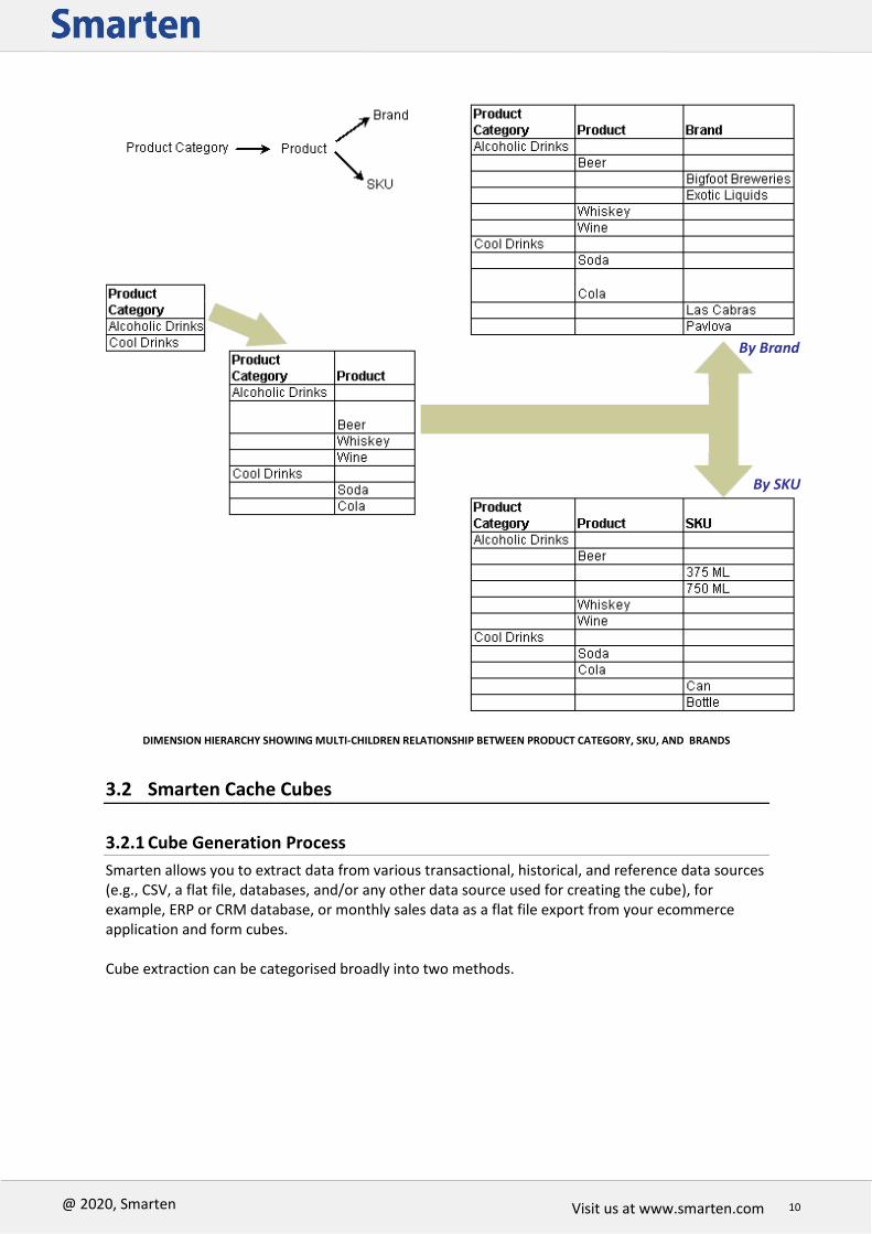
3.2.5.1 UNION
CUBE RESULTING FROM UNION QUERY
3.2.5.2 JOIN
CUBE RESULTING FROM JOIN QUERY
Here two cubes containing customer details and product details are merged
to form a single cube containing customer & sold product details by means
of a common field Order ID using JOIN query
Customer.OrderID
=
Product.OrderID

Visit us at www.smarten.com 20
@ 2020, Smarten
Visit us at
3.2.6 Supported Data Types
A cube is formed from data sets that contain various data types. Examples of data types and usage:
Data type Description Example
String A sequence of characters, usually forming a part of text
Hello, World
Integer A whole number that includes all negative numbers, zero, and all positive numbers
10
Double Numbers with decimals 12.345
Date Various date formats/expressions are possible for measuring date
15/07/2014 (dd/MM/yyyy) September 15 (MMMM dd) September 15, 2014 (MMMM dd, yyyy)
Time Used for measuring time
07:45:40 HH:mm:ss or 07:45 HH:mm
Timestamp Combination of date and time data types September 15, 07:45:40 (MMMM dd, HH:mm:ss) 09-15-2014 07:45:40 (MM-dd-yyyyHH:mm:ss)
Boolean Values with only zero and one 1 (if True) and 0 (if False)
Bit Values generated in Bit format by any system
1 and/or 0
Note:
Some of the data types that require to store large data types, such as Blob-data type, will
store cube columns with null values, i.e., these values will not be stored in cube data files.

Visit us at www.smarten.com 21
@ 2020, Smarten
Visit us at
3.3 Smarten Real-Time Cubes
Smarten offers real-time analytics through its real-time cube architecture. Real-time analytics is required in various use cases, such as the stock market, telecommunications, IT infrastructure management, and IoT, where recent data is important, and users need to access data in real time. The Real-Time Data Connector does not store or cache any data in the cubes. It extracts the data from data sources as and when required and always retrieves the latest data from data sources. It connects to JDBC / ODBC-compliant relational databases, such as Microsoft® SQL Server, Oracle, and MySQL.
SMARTEN—REAL-TIME CUBE SYSTEM ARCHITECTURE
The Smarten Real-Time cube connector provides two ways to connect to a database:
1) through graphical UI wizard 2) through paste query option
The Smarten real-time cube connector through wizard allows the user to select databases, tables, and columns, and define relationships by a drag and drop interface. The Smarten real-time cube connector through paste query allows users to paste a generated query. Users can access real-time cubes in Smarten by the following steps:
Create Database Profile / Use existing database profile
Define Real-Time Cube Profile
Access Real-Time cubes from Smarten front-end tools Create Data Source Profile: Users can enter required configuration parameters, such as driver name, URL, user name, and password. It validates the connection and creates the database profile in the system.

Visit us at www.smarten.com 22
@ 2020, Smarten
Visit us at
Define Real-Time Cube: To define the real-time cube profile, users can select the database profile created in the above step. After selecting the database profile, the system will connect to the data source and provide easy-to-use steps to define the real-time cube metadata profile within Smarten.
Configuration of database profile using JDBC/ODBC driver
Connection with database
Design SQL statement in two ways: o Graphical Query Designer o SQL Query in editor
Metadata definition for cube by designing and mapping data source columns and cube dimension and measure columns
Define Dimension Map Hierarchy Access Real-Time Cubes from Smarten front-end tools: Users can access real-time cubes from front-end objects, such as dashboards, crosstab, tabular, graphs, GeoMap and KPI. SQL queries are formed dynamically based on user actions from BI front-end tools, e.g., outliner settings or add column from analysis. Dynamically generated SQL queries are sent for execution to SQL executor, and database engine returns query results, which are then processed and displayed to the user. Please note here that cube and analytic functions available to users depend on the type of cube used in a particular front-end object. Refer to the user manual for a list of functions available while using real-time cubes.
3.4 Cube & Object Management
3.4.1 Matching Cube Criteria
Users, especially technical users, may need to associate objects (e.g., crosstab or tabular or a graph) created from one cube to another cube. It is possible to associate an object with another cube if the columns of original cube from which the object was created is matching the columns of new cube. Criteria for identical match for columns (dimensions, measures, custom cube dimensions, custom cube measures, and dimension hierarchies) are described below.
The Datatype of Dimensions in both cubes must be same. For example, if anlaysis1 is using dimension1 from Cube1, and dimension1 is of string data type, it can be matched with any dimension having string data type from target cube.
Target cube should have at least one unique matching dimension for each dimension used in the object. For example, if graph1 is using dimension1 (date type) and dimension2 (string type) from Cube1, matching target cube must have at least one date data type dimension and one string data type dimension.
One to one relationship between dimensions from target cube and dimensions used in objects. For example, if dimension1 of an object, is matched with dimensionx of target cube, dimension cannot be matched with any other dimension of the object.
Any measure of an object will match with any measure from the target cube, as datatypes of measures are always the same.
One measure in target cube can be associated with multiple measures from the object. For example, measurex of target cube can be associated with measure1 and measure2 of analysis1.

Visit us at www.smarten.com 23
@ 2020, Smarten
Visit us at
3.4.2 Assigning Objects to another matching cube
Users can assign any or all objects (crosstab, tabular, graphs, GeoMap and KPI) of one cube (including the objects with deleted cube) to matching columns of another cube.
Note:
You can associate object created from one type of cube with any other type of cube. For
example, you can associate a crosstab created from cache cube with real-time or MDX cube.
3.4.3 Copy cube
This feature enables users to copy a cube with its metadata and tool templates. This feature will copy a cube with its metadata and tool templates. This will improve the process of replicating cubes and the reusability for a template-driven deployment process. For example, if you have created a sales cube and want to replicate this cube for a different zone wise groups of users, you can create zone wise copies of this sales cube (e.g., sales cube zone1, sales cube zone2, etc.) and provide access rights to these cubes to different groups of users (e.g., zone1 users, zone2 users, etc.). You do not need to go through a cube creation process for each zone.
3.4.4 Renaming the Cubes
This feature enables users to rename the cube. Please consider a scenario. For example, the IT team is designing, developing, and testing various cubes and analysis objects on the development server. They created a cube and named it “Sales-Development-Server-Cube.” Various crosstabs, graphs, GeoMaps, dashboards, and tabular are generated. Once testing and verification are done, the “Sales-Development-Server-Cube” and the associated objects of this cube are moved or copied to the production server, and the cube is renamed “Sales-Cube” from “Sales-Development-Server Cube.” All analysis objects on the production server are now associated to “Sales-Cube” on the production server rather than “Sales-Development-Server-Cube.” So renaming avoids redeveloping or redesigning any cubes or objects. Once the cube is renamed, the modified cube name would automatically be reflected in the associated objects.
3.4.5 Renaming the Objects
This feature allows users to modify an object (crosstabs, KPI, tabular, graphs, GeoMap and dashboard) name. You can rename the objects even if the cube associated with these objects is deleted. Consider a scenario. The crosstab generated from the Sales-Development-Server-Cube is named “Development Server-Sales Analysis” during the development and testing phase. Once the cube and this crosstab move to the production server, the crosstab is renamed “Sales Analysis” without affecting its association with Sales-Development-Server-Cube.
3.4.6 Deleting the Cube without deleting dependent Objects
If a cube is deleted, user may or may not delete objects associated with that cube.

Visit us at www.smarten.com 24
@ 2020, Smarten
Visit us at
Users can reuse the dependent objects (without cube) by associating these objects to any other matching columns of another cube. Smarten saves the profile of the deleted cube. Cube metadata, such as dimensions, measures and other parametric information, remains available in the system for reference. Once a cube profile is permanently deleted, the Cube Profile and the metadata will no longer be available in the system.
3.5 Supported Features for Different Cubes
Following table specifies the feature availability for different cube types.
3.5.1 Cube Management Functions
Features Smarten Cache Cubes
Smarten Real-Time Cubes
MDX SSAS Cubes
Profile Creation ✔ ✔ ✔
Cube Creation ✔ ✔ ✔
Storing transactional and aggregate data on Smarten
✔ ✘
✘
Managed Memory Computing ✔ ✘ ✘
Cube Rebuild (Meta data update) ✔ ✔ ✘
Cube Rebuild (Data refresh) ✔ NA NA
Linked Cube ✔ ✘ ✘
Dimension Map
Retrieval of dimension maps created on cube server
NA NA ✔
User defined dimension maps in Smarten
✔ ✔
✔
Retrieval Parameters ✔ ✔ ✔
Use of Global variable in database query for rebuilding cubes
✔ ✔
✘
Use of Predefined system level global variable ‘$currentuser$’ in database query for cubes
✘ ✔
✘
Custom Cube Dimension/Measure ✔ ✘
Column Access Permission ✔ ✔ ✔
Data Access Permission ✔ ✔ ✔
Data Display Value Mapping ✔ ✔ ✔

Visit us at www.smarten.com 25
@ 2020, Smarten
Visit us at
3.5.2 Analytic Functions
Features Smarten Cache Cubes
Smarten Real-Time
Cubes
MDX SSAS
Cubes
Slice and Dice ✔ ✔ ✔
Drill Down & Drill Up ✔ ✔ ✔
Drill Through ✔ ✔ ✔
Retrival Parameters ✔ ✔ ✔
Global Variables ✔ ✔ ✔
Time Series
Absolute ✔ ✔ ✔
Relative Full Period ✔ ✔ ✔
Period-To-Date ✔ ✔ ✔
Range ✔ ✔ ✔
Outliner Filter / Page Dimension Filter
On String Column
Particular Value ✔ ✔ ✔
Value Starts with/Ends with/Contains/Null/Not Null
✔ ✔ ✘
Value within range
✔ ✔
✔
Multiple Values ✔ ✔ ✔
On Numeric Column
Particular Value ✔ ✔ ✔
Value Greater than/Less than/Greater than equal to/Less than equal to/Null/Not Null
✔ ✔ ✔
Value within range
✔ ✔ ✔
Multiple Values ✔ ✔ ✔
on Date Column
Particular Value ✔ ✔ ✔
Value Before/After/Between/Not Between
✔ ✔ ✔
Cell Filter ✔ ✔ ✔
Advanced Filter ✔ ✔ ✔
Show / Hide ✔ ✔ ✔
Analysis Title ✔ ✔ ✔
Edit Label Text in Row, Column and Data Headers ✔ ✔ ✔
Supress Zeros in Row / Column ✔ ✔ ✔
Sort
General Sort ✔ ✔ ✔
Custom Sort ✔ ✔ ✔
Advanced Sort ✔ ✔ ✘
Rank ✔ ✔ ✔
Group / UnGroup ✔ ✔ ✔
SpotLighter ✔ ✔ ✔

Visit us at www.smarten.com 26
@ 2020, Smarten
Visit us at
Data Value / Display Value Mapping ✔ ✔ ✔
Data Operation
None ✔ ✔ ✔
Sum Average Effective Average Count Effective Count Maximum Minimum First Last Distinct Count Distinct Sum Distinct Average Least Recent Values Most Recent Values
✔ ✔ ✘
Row Percentage Row Group Percentage Column Percentage Column Group Percentage Total Percentage Relative Row Difference Relative Row Difference Percentage Relative Row Group Difference Relative Row Group Difference Percentage Relative Column Difference Relative Column Difference Percentage Relative Column Group Difference Relative Column Group Difference Percentage Row Cumulative Sum Column Cumulative Sum Row Group Cumulative Sum Column Group Cumulative Sum
✔ ✔ ✔
Summary Operation Default ✔ ✔ ✔

Visit us at www.smarten.com 27
@ 2020, Smarten
Visit us at
Sum Average Effective Average Count Effective Count Maximum Minimum First Last
✔ ✔ ✘
Group Sum Group Average Group Count Group Maximum Group Minimum Row Percentage Row Group Percentage Column Percentage Column Group Percentage Total Percentage Relative Row Difference Relative Row Difference Percentage Relative Row Grop Difference Relative Row Group Difference Percentage Relative Column Difference Relative Column Difference Percentage Relative Column Group Difference Relative Column Group Difference Percentage Row Cumulative Sum Column Cumulative Sum Row Group Cumulative Sum Column Group Cumulative Sum
✔ ✔ ✔
Notes ✔ ✔ ✔
Format Component Properties ✔ ✔ ✔
Add / Remove Columns ✔ ✔ ✔
Add Custom Measure (UDDC) ✔ ✔ ✔

Visit us at www.smarten.com 28
@ 2020, Smarten
Visit us at
Add Custom Dimension Value (UDHC) ✔ ✔ ✔
What-If Analysis ✔ ✔ ✔
SubView ✔ ✔ ✔
Master-Detail view in Tabular report ✔ ✔ ✔
Auto Generate Graph from Analysis ✔ ✔ ✔
Export Analysis ✔ ✔ ✔
Save Analysis ✔ ✔ ✔
Refresh Analysis ✔ ✔ ✔
Delivery & Publishing Agent – [Publish Now] and [Publish Settings]
✔ ✔ ✔
Operations Summary ✔ ✔ ✔
Printing Analysis ✔ ✔ ✔
Page Preview ✔ ✔ ✔
Note:
Cube type should be selected based on the use case.
Reference: Impact-of-Cube-Design-on-Performance > Cube type selection recommendations

Visit us at www.smarten.com 29
@ 2020, Smarten
Visit us at
4 Analytic Functions
Various analytic functions are available to help users effectively analyse data within various Smarten modules. All functions may not be available in all modules, e.g., summary operations are not available in graphs and GeoMap.
4.1 Slice & Dice
“Slice & Dice” describes the functions at the core of OLAP analysis. The multidimensional tools allow users to view data from any angle. Through slice & dice, user can rotate the presentation between rows and columns in crosstabs. After generating a crosstab, graph, or tabular, a user swaps dimensions from row to column and column to row.
SLICE AND DICE PRODUCT CATEGORY AND REGIONWISE SALES
4.2 Drill down and Drill up
“Drill down” and “Drill up” provide interactive data analysis through predefined dimension hierarchy. In hierarchical drilling, user can interactively retrieve data at multiple levels. User can move down and up the hierarchies to see how the information at various levels is related.
4.2.1 Drill down
“Drill down” interactive data analysis allows users to navigate from less-detailed aggregated information to view more granular data. After looking at the gross sales for a state, user may wish to see the individual sales for each city of that state.

Visit us at www.smarten.com 30
@ 2020, Smarten
Visit us at
4.2.2 Drill up
It refers to the process of navigating information from the detailed (down) to the summarized (up) along a dimension hierarchy. For example, when viewing the data for the city of Miami, a drill-up operation in the location dimension would display Florida. A further drill up on Florida would display data for the USA.
DRILL DOWN AND DRILL UP DATA ANALYSIS
Drill down / Drill up can be based not only on predefined dimensional hierarchy, but the user can also add unrelated child levels to a parent node to see the bifurcation of the aggregated information regardless of predefined hierarchy defined at cube levels. For example, we can see sales by employees for any given state even if state/employee hierarchy is not defined in the dimension map in the cube. Add employees to the drill-down level of states as shown in the figure below.
DRILL DOWN AND DRILL UP OF EMPLOYEE SALES BY STATE

Visit us at www.smarten.com 31
@ 2020, Smarten
Visit us at
4.3 Drill Through
Using “drill through” on analysis retrieves the detailed row or transaction level data from which the data in the cube cell was summarized. It is used to access the underlying transactional or row-level view of selected analysis columns / row or cell. For example, user can see all transactions contributing to GrossSales of 1643997 for Alcoholic Drinks in January.
DRILL THROUGH
If cube created with only “Store drill through data” option then drill though data retrieves from Flat cube data. If cube created with only “Perform aggregation” option then drill through data retrieves from Aggregated data of cube. If cube created with both “Store drill through data” and “Perform aggregation” options then based on the different scenarios drill through data retrieves from the “Flat data” or “Aggregated data” of the cube. If an object being used for drill through is using any custom cube column (custom cube dimension or custom cube measure), then drill through data will be displayed from the aggregated data of the cube. If an object being used does not use any custom cube column, then drill through data will be displayed from flat cube data.
State City Product Category
Product Quantity Production Cost
Packing Cost
Arizona Phoenix Bakery Bread 150 300 30
Arizona Phoenix Bakery Bread 200 400 40

Visit us at www.smarten.com 32
@ 2020, Smarten
Visit us at
Arizona Phoenix Bakery Bun 160 480 48
Arizona Phoenix Bakery Bun 200 600 60
Arizona Phoenix Cool Drinks Soda 200 1000 60
Arizona Phoenix Cool Drinks Soda 180 720 54
Arizona Scottsdale Bakery Bread 400 1200 80
Arizona Scottsdale Bakery Cookies 300 900 60
Arizona Scottsdale Bakery Bun 250 750 75
Arizona Scottsdale Bakery Bun 200 600 60
Arizona Scottsdale Cool Drinks Cola 180 900 54
Arizona Scottsdale Cool Drinks Cola 190 760 57
Florida Miami Bakery Bread 200 400 40
Florida Miami Bakery Bread 250 500 50
Florida Miami Bakery Bun 150 450 45
Florida Miami Bakery Bun 200 600 60
Florida Miami Cool Drinks Cola 170 850 51
Florida Miami Cool Drinks Soda 150 600 45
Florida Orlando Bakery Bread 270 540 54
Florida Orlando Bakery Bun 180 540 54
Florida Orlando Cool Drinks Cola 190 950 57
Florida Orlando Cool Drinks Cola 200 1000 60
Florida Orlando Cool Drinks Soda 170 680 51
Florida Orlando Cool Drinks Soda 210 840 63
FLAT DATA SET
Custom cube column
State City Product Category
Product Qty Production Cost
Packing Cost
Total Cost
Arizona Phoenix Bakery Bread 350 700 70 770
Arizona Phoenix Bakery Bun 360 1080 108 1188
Arizona Phoenix Cool Drinks Soda 380 1720 114 1834
Arizona Scottsdale Bakery Bread 400 1200 80 1280
Arizona Scottsdale Bakery Cookies 300 900 60 960
Arizona Scottsdale Bakery Bun 450 1350 135 1485
Arizona Scottsdale Cool Drinks Cola 370 1660 111 1771
Florida Miami Bakery Bread 450 900 90 990
Florida Miami Bakery Bun 350 1050 105 1155
Florida Miami Cool Drinks Cola 170 850 51 901
Florida Miami Cool Drinks Soda 150 600 45 645
Florida Orlando Bakery Bread 270 540 54 594
Florida Orlando Bakery Bun 180 540 54 594
Florida Orlando Cool Drinks Cola 390 1950 117 2067
Florida Orlando Cool Drinks Soda 380 1520 114 1634
AGGREGATED DATA SET WITH CUSTOM CUBE COLUMN “TOTAL COST”
Custom cube column Total Cost = Production Cost + Packing Cost Scenario 1: Crosstab does not use any custom cube column, and no custom cube column is selected in drill through.

Visit us at www.smarten.com 33
@ 2020, Smarten
Visit us at
FLAT DATA IN DRILL THROUGH
In such a scenario, flat cube data will be displayed in drill through view. Scenario 2: Crosstab uses any custom cube column, and no custom cube column is selected in drill through.
AGGREGATED DATA IN DRILL THROUGH
In such a scenario, aggregated cube data will be displayed in drill through view. Scenario 3: Crosstab uses any custom cube column, and custom cube column is selected in drill through.

Visit us at www.smarten.com 34
@ 2020, Smarten
Visit us at
AGGREGATED DATA IN DRILL THROUGH
In such a scenario, aggregated cube data will be displayed in drill through view. Scenario 4: Crosstab does not use any custom cube column, but custom cube column is selected in drill through.
AGGREGATED DATA IN DRILL THROUGH
In such a scenario, aggregated cube data will be displayed in drill through view.
4.4 Global Variables
The global variables are defined at the cube level. They can be accessed globally with various expressions and filters for BI objects within Smarten. For example, users need to view the projection of growth based on variable % values of sales amount. For this, a Custom Measure Column (UDDC) Growth can be created that would be calculated on the basis of a variable X and GrossSales. This X can be created as a Global Variable and assigned different values at different times to evaluate various scenarios. Formula for Growth: GrossSales + (X*GrossSales)/100 Users can change the value of X to see different projections of growth. Any change in X would be reflected in all analyses where the value of X is used through different expressions in filters, the Custom Dimension Value (UDHC), the Custom Measure Column (UDDC),

Visit us at www.smarten.com 35
@ 2020, Smarten
Visit us at
and retrieval parameters. Hence, it saves users from the tedious task of modifying various expressions and filter formula manually and provides simple “what if” analysis scenarios. Once the global variable is defined, it would be accessible throughout the application while applying Filters, creating Custom Dimension Value (UDHC), Custom Measure Column (UDDC), and Retrieval Parameters. Users can also use these global variables in cube query while rebuilding Cache or Real-Time cubes. User can also use the predefined system level global variable ‘$currentuser$’ in Real-Time cube query. For example, user can create a real time cube using query "Select * from Sales where
employeename = ‘$currentuser$’". In this scenario, if user1 is logged in and is using real time cube
data, query expression will be: “Select * from Sales where employeename = ‘User1’, and if user2 is
logged in and is using this real time cube data, query expression will be: “Select * from Sales where
employeename = ‘User2’.
Note:
Global variables are available within all BI objects (such as crosstab, graph, GeoMap,
dashboards, and tabular) created from a cube. Global variables created for one cube cannot
be accessed from within objects created from another cube.
CUSTOM MEASURE COLUMN (GROWTH) DERIVED USING GLOBAL VARIABLE X (VALUE: 15)

Visit us at www.smarten.com 36
@ 2020, Smarten
Visit us at
CUSTOM MEASURE COLUMN (GROWTH) DERIVED FROM MODIFIED VALUE OF GLOBAL VARIABLE X (VALUE: 20)
The value of global variable X is modified from 15 to 20. In the column Growth, new value 20 will be taken into consideration, and column values will change accordingly.
Note:
The global variables will be available for such objects as crosstabs, graphs, GeoMap, tabular,
and KPIs.

Visit us at www.smarten.com 37
@ 2020, Smarten
Visit us at
4.5 Show only Summary data
This feature is useful in scenarios when a user wants to see only summary row(s) for a group of rows / columns without displaying the actual rows / columns in crosstab or tabular. For example, if the user wants to view the total number of customers for each product category without displaying the customer details, they can use the Group Count Function to display that and select “Show Only Summary Data” option. This feature is rather helpful to users when they need to display the group summary operations, such as group count, group average, group maximum, group minimum, etc., in this fashion.
BEFORE: PRODUCT CATEGORYWISE & EMPLOYEEWISE SALES WITH
PRODUCT CATEGORYWISE NUMBER OF EMPLOYEES

Visit us at www.smarten.com 38
@ 2020, Smarten
Visit us at
AFTER: PRODUCT CATEGORYWISE NUMBER OF EMPLOYEES
WITHOUT DISPLAYING CATEGORYWISE SALES
4.6 Sort
Data can be sorted in ascending, descending, and custom (user defined) orders, using particular Dimension or Measure fields.
4.6.1 Simple Sort
Simple sorting in ascending or descending order.
SORT BY PRODUCT CATEGORY AND SALES QUANTITY
User can also use “Advanced Sort” to sort dimension based on a data operation on a particular measure.

Visit us at www.smarten.com 39
@ 2020, Smarten
Visit us at
4.6.2 Advance Sort
Applying filter conditions for sorting of the data—Advance Sorting User can also apply sorting of data by using various data operations on particular measure. For example, user can sort ProductCategory column in “descending” order on the Sum of GrossSales for the state of Arizona.
Advance filtering can be applied on data column using data operations, such as Sum, Average, Effective Average, Count, Effective Count, Ineffective Count, Minimum, and Maximum.
DATA SORTED ON THE PRODUCT CATEGORY DIMENSION VALUES
ANALYSIS AFTER APPLYING THE ADVANCE SORTING ON THE “PRODUCTCATEGORY” COLUMN IN “DESCENDING” ORDER ON “SUM” DATA OPERATION OF “GROSSSALES” DATA COLUMN FOR THE STATE “ARIZONA.”
Visit us at www.smarten.com 40
@ 2020, Smarten
Visit us at
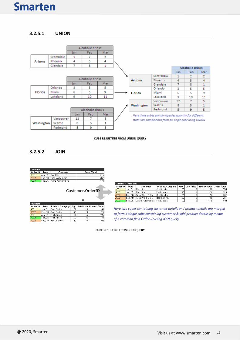
4.6.3 Custom Sort
Users can also sort data in custom order based on specific requirements.
FILTERING RESULTS BASED ON CUSTOMIZED SORTING

Visit us at www.smarten.com 41
@ 2020, Smarten
Visit us at
4.7 Group & Ungroup
Merging and demerging the data based on logical groups is known as Packing/Unpacking. Grouping is used to merge selective cells into one cell. Ungrouping can be used to demerge the grouped data.
GROUPED & UNGROUPED DATA

Visit us at www.smarten.com 42
@ 2020, Smarten
Visit us at
4.8 Spotlighter
Spotlighting is used to highlight specific values based on certain conditions to identify exceptions and variations in a quick glance. For example, to indicate the sales quantity fields with value less than 4000000 as “low” and also to change the field background colour, Spotlighting can be used.
SPOT LIGHTER SHOWING ALERTS ON LOW SALES
Note:
User can display static or dynamic text as alternate text for the spotlighted cells. Dynamic text
will allow users to display alternate text using expressions. These expressions can be based on
the columns used in the spotlighter configuration, e.g., $GrossSales – Low and $GrossSales –
High in respective spotlighters will display actual Gross Sales amount, concatenate with word
“Low” or “High” based on spotlighter condition, i.e., 363390 – Low, 21361087 – High.
User can apply spotlighter with multiple conditions, such as GrossSales greater than 40,00,000 and less than 90,00,000 as shown below.

Visit us at www.smarten.com 43
@ 2020, Smarten
Visit us at
SPOTLIGHTER WITH MULTIPLE CONDITION
ANALYSIS BEFORE AND AFTER SPOTLIGHTER WITH MULTIPLE CONDITION

Visit us at www.smarten.com 44
@ 2020, Smarten
Visit us at
The spotlighter can be applied on data or on the row or column summaries as well as simultaneously on the data and the summaries.
THE OPTIONS TO APPLY THE SPOTLIGHTER ON DATA, ROW SUMMARY, COLUMN SUMMARY, OR ALL
ANALYSIS BEFORE AND AFTER SPOTLIGHT ON THE
DATA, ON ROW SUMMARY, AND ON COLUMN SUMMARY
Note:
Please note that a Spot lighter created from crosstab or tabular cannot be used in GeoMap
and vice versa.

Visit us at www.smarten.com 45
@ 2020, Smarten
Visit us at
4.9 Data Value / Display Value mapping
Data value / Display value mapping can display alternate text for specific field values. Displayed data (row/column) names (column headings) can be changed based on data values. For example, if quarters are available as numbers 1 to 4 (e.g., 1 for Quarter1, 2 for Quarter2), the user can specify display value for the corresponding data values from the cube. Users can view the quarter names instead of quarter numbers for a user-friendly experience.
DATA VALUE/ DISPLAY VALUE MAPPING

Visit us at www.smarten.com 46
@ 2020, Smarten
Visit us at
4.10 UDDC & UDHC
4.10.1 Custom Measure (UDDC)
The custom measures in Smarten are easy to build. They can be created by building a formula on existing columns according to the crosstab or tabular requirements. The custom measures are also known as User Defined Data Columns (UDDC). Users can create custom measure columns from existing measures by performing various string, arithmetic, date, statistics, trigonometry, or conditional statements using various arithmetic operators (such as +, -, /, etc.) or comparison operators (such as =, >, < etc.).
CUSTOM MEASURE (UDDC)
Here, Growth is a Custom Measure derived from an operation on the measures Sales (Q4-2013) and Sales (Q3-2013). Growth would be available to all users as a ready-to-use measure. Custom measures can also be created using other custom cube dimensions and measures. For example, users can create another Custom Measure, GrowthPercentage by taking 5% of GrossSales. Here, the input measure is GrossSales, which is itself a Custom Measure. Custom measures can also be created in graphs and GeoMap.
Note:
If UDDC is created from other columns (source columns) in the cube and the user is not
granted privileges to access source columns but is granted privileges to access the resultant
column, the user will be able to access the resultant column.
For example, if a UDDC “Total_Price” is created by using the expression: Total_Price = Qty *
Rate and the user is not granted access rights for Qty and / or Price column but does have
rights for Total_Price, the user will be able to access the Total_Price column.
UDDC is created on front-end data by users and not on cube data (aggregated result set of a
cube). It can be used in crosstab, tabular, graphs, GeoMap and KPIs.

Visit us at www.smarten.com 47
@ 2020, Smarten
Visit us at
4.10.2 Custom Dimension Value (UDHC)
Custom dimension value columns or rows can be created by defining and applying mathematical formulae on existing row and column values as per your needs. This is also known as User Defined Header Columns (UDHC). Users can create new dimension value columns by performing various conditional statements, such as string, arithmetic, date, statistics, trigonometry, or using various arithmetic operators (such as +, -, /, etc.) or comparison operators (such as =, >, < etc.) on two or more existing dimension columns or rows. Users can also create custom dimension values by performing valid operations on existing dimensions.
CUSTOM DIMENSION VALUE (UDHC)
Product categories Cold Drinks, Fruit Juices, Health Drinks, and Tea can be grouped as “Nonalcoholic Drinks.”
Note:
UDHC is created on front-end data by users and not on cube data (aggregated result set of a
cube). It can be used in crosstab, tabular and graphs.
Please note that a UDHC cannot be used in KPI and GeoMap.

Visit us at www.smarten.com 48
@ 2020, Smarten
Visit us at
Calculation Priority over Custom Measure: Users can choose the calculation priority among UDDC and UDHC while creating UDHC. For example: There is a Custom Measure (UDDC) column created with formula “X” (where X = rowGroupPercentage [Measure]). When users create a Custom Dimension (UHDC) with Formula “Y” (where Y = row 1 + row 2), they can have an option to prioritize the value to be displayed at the intersection cell as per formula X (based on UDDC) OR as per formula Y (based on UDHC). In the example below for the UDHC “AA,” the UDDC formula is: rowGroupPercentage (GrossSales), and the UDHC formula is: (State_Arizona + State_Arkansas).
INTERSECTION VALUE AFTER SELECTING THE PRIORITY OVER UDDC
In this instance, 76% margin is calculated based on UDHC formula for the year 2014.
INTERSECTION VALUE WITHOUT SELECTING THE PRIORITY OVER UDDC
In this instance, 37% margin is calculated based on UDDC formula for the year 2014.
Note:
If UDDC or UDHC is created from other columns (source columns) in the cube and the user is
not granted privileges to access source columns but is granted privileges to access the
resultant column, the user will be able to access the resultant column.
For example, if a UDDC “Total_Price” is created by using the expression: Total_Price = Qty *
Rate and the user is not granted access rights for Qty and / or Price column but does have
rights for Total_Price, the user will be able to access the Total_Price column.

Visit us at www.smarten.com 49
@ 2020, Smarten
Visit us at
4.10.3 Cell referencing in UDDC & UDHC
Cell Referencing allows users to reference a particular cell in a report and use it in user-defined data column (UDDC) and user-defined header column (UDHC) expressions.
Naming Convention of cells
A cell reference consists of Row and Column numbers that intersect at a cell’s location.
NAMING CONVENTION OF CELLS
The GrossSales for Alcoholic Drinks, Arizona is referred to as R1C1 since it is at the intersection of the first Row (R1) and the first column (C1). The GrossSales for Fruit Juices, Florida is referred to as R5C3 since it is at the intersection of the fifth Row (R5) and the third column (C3). The cell reference is not adjusted with the change of cell position based on updates in data or redesign of the report. Here, position associated with a cell is taken as a static position based reference rather than relative position based reference that keeps moving based on changed cell positions. For example,
To refer the GrossSales of Bakery, Arizona the position based cell reference is Second row, First column - R2C1 with value 10197878. Suppose, on the cube update, a row (Aerated Drinks) is inserted.

Visit us at www.smarten.com 50
@ 2020, Smarten
Visit us at
Once an additional row is inserted, R2C1 will now refer to (second row, first column), that is the GrossSales of Alcoholic Drinks, Arizona which is 6415757. To refer the GrossSales of Bakery, Arizona the cell reference provided has to be R3C1. So, as R2C1 is referred with static cell position based referencing, and it will assume new value of cell based on static cell position after cube updates or report redesign. There are two types of cell references –Absolute and Relative cellreferencing. Absolute Cell Referencing Absolute cell referencing refers to the absolute position of a cell. For absolute cell referencing, a cell reference should include a $ sign before the column number and / or row number. $ indicates that cell reference is Absolute; it will always refer to the same position of cell (e.g., $R2$C1 - second row, first column, in all cases). For example,
To refer to the GrossSales of Bakery, Arizona, the cell reference is $R2$C1 with value 8347787. Suppose, on the cube update, a row (Aerated Drinks) is inserted.

Visit us at www.smarten.com 51
@ 2020, Smarten
Visit us at
Once an additional row is inserted, $R2$C1 will now refer to the second row, first column of the report, that is, the GrossSales of Alcoholic Drinks, Arizona, which is 5679096. To refer to the GrossSales of Bakery, Arizona, the cell reference provided has to be $R3$C1. So, with this new data update, $R2$C1 will return a value of 5679096 - GrossSales of Alcoholic Drinks, Arizona instead of 8347787 - GrossSales of Bakery, Arizona.
Relative Cell Referencing Relative cell referencing refers to the position of a cell in relation to the current row or column being considered for the calculation. Relative cell reference expression does not include a $ sign. For example, R2C1 refers to the value at second row and first column. For example, there is no column dimension defined in the report. In this case, you have just one column (C1 - Gross Sales) in the report, and you are adding second column (C2) in an existing report.
The UDDC expression to be defined for C2 will be written for new column’s cell at first row (R1), that is C2R1 if you are creating second column (C2), or C3R1 if you are creating third column (C3) in the report. For the UDDC expression, the expression is always written with reference position to the topmost left cell of the report, that is always R1C1 in any report.
To summarise this, if you are creating second column (C2) in the report, UDDC expression will be written for expression for cell R1C2, and expression will contain reference to R1C1. If you are creating forth column (C4) in the report, UDDC expression will be written for expression for cell R1C4, and expression will contain reference to R1C1. In the example above following expressions are used. C2 = R2C1 means, defining value of R1C2. C3 = R2C1 – R1C1 means, defining value of R1C3.

Visit us at www.smarten.com 52
@ 2020, Smarten
Visit us at
C2=R2C1 means that R1C2 will have value of R2C1. That means, current cell value should be fetched from cell that is one row below (from R1 to R2) and column that is one column left (from C2 to C1). C3= R2C1 – R1C1 means that R1C3 will have value of subtraction of R1C1 from value of R2C1. In reference to current cell R1C3, R2C1 is a cell from one row below (from R1 to R2) and column that is two columns left (from C3 to C1). And in reference to R1C3, R1C1 is a cell from same row (from R1 to R1) and column that is two columns left (from C3 to C1). Now, if you have report with column dimension, same scenario will be replicated for all repeated column dimensions. E.g. Arizona represents first column dimension value, and Arkansas represents second column dimension value. In this case, C1 represents Sales Amount of Arizona, and C2 represents sales amount of Arkansas.
If you add new UDDC (C2), then two UDDC columns – C2 for Arizona, and C4 for Arkansas will be created as below.
The logic explained above for report without column dimension, will be replicated across all column dimensions in the report. So, logic explained for C2 in report without column dimension, will be replicated for C4, C6, and so on, depending on number of column dimension values.

Visit us at www.smarten.com 53
@ 2020, Smarten
Visit us at
Building Expressions (Absolute and Relative Cell Referencing) You can build formulas based on the absolute and relative cell referencing techniques explained above. While building expressions, all formulas are written with reference to R1C1 – first row, first column. The reference to position of row and column is based on relative value (without $ sign) and absolute (with $ sign) reference in the expression. The table below illustrates some examples.
Cell Reference Expression Value
Absolute Row, Absolute Column [$Rx$Cy]
$R1$C3 Both the row and column references are absolute. Expression will always return value of the cell in first row and third column.
$R3$C1 Both the row and column references are absolute. Expression will always return value of the cell in third row and first column.
Relative row, Absolute column [Rx$Cy]
R1$C3 Column value will remain absolute and row value will change with reference to the position of current cell. Expression will return value of the cell in third column and current row position. For example, if C2 is being created, R1C2 will represent value of R1C3, and R2C2 will represent value of R2C3 and so on. If C4 is being created, R1C4 will represent value of R1C3, and R2C4 will represent value of R2C3 and so on.
R3$C1 Column value will remain absolute and row value will change with reference to the position of current cell. Expression will return value of the cell in first column and third row from the current row position. For example, if C2 is being created, R1C2 will represent value of R3C1, and R2C2 will represent value of R4C1 and so on. If C4 is being created, R1C4 will represent value of R3C1, and R2C4 will represent value of R4C1 and so on.
Absolute row, relative column [$RxCy]
$R1C3 Row value will remain absolute and column value will change with reference to the position of current cell. Expression will return value of the cell in third column from current column and first row position. For example, if C2 is being created, R1C2 will represent value of R1C3, and R2C2 will represent value of R1C3 and so on. If C4 is being created, R1C4 will represent value of R1C5, and R2C4 will represent

Visit us at www.smarten.com 54
@ 2020, Smarten
Visit us at
value of R1C5 and so on.
$R3C1 Row value will remain absolute and column value will change with reference to the position of current cell. Expression will return value of the cell in first column from current column and third row position. For example, if C2 is being created, R1C2 will represent value of R3C1, and R2C2 will represent value of R3C1 and so on. If C4 is being created, R1C4 will represent value of R3C3, and R2C4 will represent value of R3C3 and so on.
Relative Row, Relative Column [RxCy]
R1C3 Both Row value and column value will change with reference to the position of current cell. Expression will return value of the cell in third column from current column and first row from current row position. For example, if C2 is being created, R1C2 will represent value of R1C3, and R2C2 will represent value of R2C3 and so on. If C4 is being created, R1C4 will represent value of R1C5, and R2C4 will represent value of R2C5 and so on.
R2C1 Both Row value and column value will change with reference to the position of current cell. Expression will return value of the cell in first column from current column and second row from current row position. For example, if C2 is being created, R1C2 will represent value of R2C1, and R2C2 will represent value of R3C1 and so on. If C4 is being created, R1C4 will represent value of R2C3, and R2C4 will represent value of R3C3 and so on.

Visit us at www.smarten.com 55
@ 2020, Smarten
Visit us at
Other examples: Absolute Row, Absolute Column [$R2$C1]
Absolute row, relative column [$R2C1]

Visit us at www.smarten.com 56
@ 2020, Smarten
Visit us at
Relative Row, Absolute Column [R1$C3]
Relative Row, Relative Column [R2C1]
User defined header column (UDHC) using cell reference. Cell referencing can be applied while creating User define header column (UDHC) also. Here the example shows state wise, city wise gross sales.

Visit us at www.smarten.com 57
@ 2020, Smarten
Visit us at
A new row is being created to show summary that shows sum of two states (Arizona and Arkansas) minus some of one state (Florida). In the new row (R10) being created, first cell value (Cell position - R10C1) should be represent difference between sum of Arizona (R3C1) and Arkansas (R6C1) and sum of Florida (R9C1). So, this formula has to be built based on absolute row reference and relative reference for current column for each moving column with new row R10. For an expression (R3C1 + R6C1) – R9C1, the calculation performed is shown below.
While creating values for new row R10, as column changes, Row (R3, R6 and R9) remains same in all cases whereas column (C1) relatively changed based on the current column location of the current cell.
4.10.4 Functions & Expressions
Arithmetic Functions
Functions Description
ABS Returns the absolute value of a number
CEIL Returns the smallest whole number that is greater than or equal to a specified number
EXP Returns the exponential value of a number
FACT Returns the factorial of a number
FLOOR Returns the largest whole number that is smaller than or equal to a specified number
LOG Returns the natural logarithm (base e) of a number
LOGTEN Returns the decimal logarithm (base 10) of a number
MAX Returns the larger of two numbers

Visit us at www.smarten.com 58
@ 2020, Smarten
Visit us at
MIN Returns the smaller of two numbers
MOD Returns the modulus of two numbers (the remainder after dividing the first number into the other number)
PI Returns pi (3.14159265358979323) times a number
RANDOM Returns a random whole number between two specified numbers
ROUND Returns a number rounded off decimal numbers
SIGN Returns a number (-1, 0, or 1) indicating the sign of a number
SQRT Returns the square root of a number
TRUNCATE Returns a number truncated to a specified number of decimal places
Date Functions
Functions Description
DatePart (period, source)
datePart( "d",dateTime( "2001-02-16 20:38:40")) Returns 16 datePart( "m",dateTime( "2001-02-16 20:38:40")) Returns 2 datePart( "y",dateTime( "2001-02-16 20:38:40")) Returns 2001 datePart( "q",dateTime( "2001-02-16 20:38:40")) Returns 1 datePart( "h",dateTime( "2001-02-16 20:38:40")) Returns 20 datePart( "n",dateTime( "2001-02-16 20:38:40")) Returns 38 datePart( "s",dateTime( "2001-02-16 20:38:40")) Returns 40 datePart( "w",dateTime( "2001-02-16 20:38:40")) Returns 7 Return Value: Returns an Integer value containing the specified component of a given Date value.
DateAdd (type, date, value)
dateAdd( "d",10,dateTime( "2001-02-16 20:38:40")) Returns 26-Feb-2001 20:38:40 dateAdd( "m",2,dateTime( "2001-02-16 20:38:40")) Returns 16-Apr-2001 20:38:40 dateAdd( "y",2,dateTime( "2001-02-16 20:38:40")) Returns 16-Feb-2003 20:38:40 dateAdd( "q",2,dateTime( "2001-02-16 20:38:40")) Returns 16-Aug-2001 20:38:40 dateAdd( "w",2,dateTime( "2001-02-16 20:38:40")) Returns 02-Mar-2001 20:38:40 dateAdd( "h",2,dateTime( "2001-02-16 20:38:40")) Returns 16-Feb-2001 22:38:40 dateAdd( "n",2,dateTime( "2001-02-16 20:38:40")) Returns 16-Feb-2001 20:40:40 dateAdd( "s",2,dateTime( "2001-02-16 20:38:40")) Returns 16-Feb-2001 20:38:42 Return Value: Returns a Date value containing a date and time value to which a specified time interval has been added.
DateDiff (type, date1, date2)
dateDiff("d", dateTime( "2001-02-18 20:38:40"),dateTime( "2001-02-16 20:38:40")) Returns 2 dateDiff("m", dateTime( "2001-02-16 20:38:40"),dateTime( "2001-05-16 20:38:40")) Returns -3 dateDiff("y", dateTime( "2003-02-16 20:38:40"),dateTime( "2001-02-16 20:38:40")) Returns 2 dateDiff("q", dateTime( "2001-07-16 20:38:40"),dateTime( "2001-02-16 20:38:40")) Returns 2 dateDiff("w", dateTime( "2001-02-18 20:38:40"),dateTime( "2001-02-06 20:38:40")) Returns 2 dateDiff("h", dateTime( "2001-02-16 20:38:40"),dateTime( "2001-02-16 10:38:40")) Returns 10

Visit us at www.smarten.com 59
@ 2020, Smarten
Visit us at
dateDiff("n", dateTime( "2001-02-16 20:38:40"),dateTime( "2001-02-16 20:18:40")) Returns 20 dateDiff("s", dateTime( "2001-02-16 20:38:40"),dateTime( "2001-02-16 20:38:10")) Returns 30 Return Value: Returns a Long value specifying the number of time intervals between two Date values.
MonthName (number1, [abbreviate], [number2])
monthName( 1,false, 1 ) Returns January monthName( 1,true, 1 ) Returns Jan Return Value: Returns a month name representing the month for a number from 1 to 12.
WeekdayName (number1, [abbreviate], [number2])
weekdayName( 2, true, 3) Returns Wed weekdayName( 2, false, 3) Returns Wednesday Return Value: Returns a day name representing the day of the week for a number from 1 to 7.
FormatDate (date, “string”)
FormatDate ('2001-02-16',’yy/mm/dd’) Returns 01/02/14 formatDate( dateTime( "2001-02-16 20:38:40"), "MM/dd/yyyy") Returns 02/16/2001 Return Value: Returns string of the specified format for a specified date.
date( object ) date( "2001-02-16") Returns 16-Feb-2001
dateTime( object ) dateTime( "2001-02-16 20:38:40") Returns 16-Feb-2001 20:38:40
day( date ) day( dateTime( "2001-02-16 20:38:40")) Returns 16
dayName ( date ) dayName( dateTime( "2001-02-16 20:38:40")) Returns Friday
dayNumber( date ) dayNumber( dateTime( "2001-02-16 20:38:40")) Returns 6
daysAfter( date , date ) daysAfter( dateTime( "2001-02-16 20:38:40"),dateTime( "2001-02-10 20:38:40")) Returns 6
hour( date ) hour( dateTime( "2001-02-16 20:38:40")) Returns 20
minute( date ) minute( dateTime( "2001-02-16 20:38:40")) Returns 38
month( date ) month( dateTime( "2001-02-16 20:38:40")) Returns 2
now() now() Returns 20:38:40 Return value : Returns current time
relativeDate( date, i ) relativeDate( dateTime( "2001-02-16 20:38:40"), 5 ) Returns Wed Feb 21 20:38:40 IST 2001 Return value: Returns the date that occurs n days after a given date
time( object ) time( "20:38:40") Returns 20:38:40
relativeTime( time , I ) relativeTime( time( "20:38:40"), 5 ) Returns 20:38:45 Return value: Returns the time that occurs n seconds after a given time
second( time ) second( time( "20:38:40")) Returns 40
today( ) today( ) Returns 16-Feb-2001 Return value: Returns the current system date
year( date ) year( dateTime( "2001-02-16 20:38:40")) Returns 2001
Statistic Functions (Only applicable for Custom Measure)
Functions Description
AVG Returns the average value of the underlying rows for a particular aggregated row
COUNT Returns the count of the underlying rows for a particular aggregated row
MAXIMUM Returns the maximum value of the underlying rows for a particular aggregated row
MINIMUM Returns the minimum value of the underlying rows for a particular aggregated row
SUM Returns the sum total of the underlying rows for a particular aggregated

Visit us at www.smarten.com 60
@ 2020, Smarten
Visit us at
row
EFFECTIVE AVERAGE Returns the effective average of the underlying rows for a particular aggregated row
EFFECTIVE COUNT Returns the effective count of the underlying rows for a particular aggregated row
ROW PERCENTAGE Returns the row percentage
ROW GROUP PERCENTAGE
Returns the row group percentage
COLUMN PERCENTAGE Returns the column percentage
COLUMN GROUP PERCENTAGE
Returns the column group percentage
TOTAL PERCENTAGE Returns the total percentage
RELATIVE ROW DIFFERENCE
Returns the relative row difference
RELATIVE ROW DIFFERENCE PERCENTAGE
Returns the relative row difference percentage
RELATIVE COLUMN DIFFERENCE
Returns the relative column difference
RELATIVE COLUMN DIFFERENCE PERCENTAGE
Returns the relative column difference percentage
ROW CUMULATIVE SUM Returns the row cumulative sum
COLUMN CUMULATIVE SUM
Returns the column cumulative sum
FIRST Returns the first value of the underlying rows for a particular aggregated row
LAST Returns the last value of the underlying rows for a particular aggregated row
DISTINCT COUNT Returns the count of unique dimension values of selected dimension from the underlying rows for a particular aggregated row
DISTINCT SUM Returns the sum of measure for unique dimension values of selected dimension from the underlying rows for a particular aggregated row
DISTINCT AVERAGE Returns the average of measure for unique dimension values of selected dimension from the underlying rows for a particular aggregated row
MOST RECENT Returns the result of different aggregation methods on most recent records from the data as per the date dimensions
LEAST RECENT Returns the result of different aggregation methods on the first records from the data as per the date dimensions
String Functions
Functions Description
ASC Returns the ASCII value of a character
BOOLEANVALUE Returns contents of a string as Boolean
BYTEVALUE Returns contents of a string as byte
CHARVALUE Returns contents of an integer as character
DOUBLEVALUE Returns contents of a string as double
FILL Returns a string of a specified length filled with occurrences of a specified string
FLOATVALUE Returns contents of a string as float
INDEXOFCHAR Returns the starting position of a character within a specified string
INDEXOFSTRING Returns the starting position of a string within a specified string

Visit us at www.smarten.com 61
@ 2020, Smarten
Visit us at
INTVALUE Returns contents of a string as integer
ISDATE Determine if the specified string contains a valid date
ISNULL Determine if the argument is NULL
ISNUMBER Determine if the specified string contains a number
ISTIME Determine if the specified string contains a valid time
LEFT Returns a specified number of characters from a string starting with the first character
LEFTTRIM Returns a copy of a specified string with leading blanks removed
LENGTH Returns length of a string
LONGVALUE Returns contents of a string as long
MATCH Returns a determination whether a string contains a particular pattern of characters
REPLACE Returns a copy of a specified string in which a specified number of characters starting with a specified character have been replaced with characters from another specified string
REVERSE Reverses the order or characters in a string
RIGHT Returns the specified number of characters from the end of a specified string
RIGHTTRIM Returns a copy of a specified string with trailing blanks removed
SHORTVALUE Returns contents of a string as short
SPACE Returns a string of a specified length filled with a specified number of spaces
SUBSTRING Returns a string containing a character copied (starting at a specified position and ending at a specified position) from a specified string
TOLOWERCASE Returns a copy of a specified string with all uppercase letters converted to lowercase
TOSTRING Returns a string representation of a specified object
TOUPPERCASE Returns a copy of a specified string with all lowercase letters converted to uppercase
TRIM Returns a string with leading and trailing blanks removed
Trigonometric Functions
Functions Description
COS Cosine of number (number in radian)
SIN Sine of number (number in radian)
TAN Tangent of number (number in radian)
Miscellaneous Functions
Functions Description
IFCASE Returns TRUE if condition is validated and returns FALSE if invalidated
WHENTHEN Tests values of a column or expression and returns values based on the results of the test
noOfDaysByDate(StartDate, EndDate)
Returns number of days between given start and end date Example: noOfDaysByDate("2014-03-10", "2014-04-10") : returns 32
noOfDaysByFrequency(PeriodFrequency, PeriodNo,isFinancialYear)
Returns number of days in a specified frequency for a given period PeriodFrequency possible values are: “y” for yearly, “h” for half yearly, “q” for quarterly, “m” for monthly, “w” weekly, and “d” for daily PeriodNo possible values are: 0 for current period, -1 for previous period, -2 for previous to previous period, and so on isFinancialYear possible values are: true for Financial year, false for Calendar year

Visit us at www.smarten.com 62
@ 2020, Smarten
Visit us at
Example: noOfDaysByFrequency(“y”,0,false) : returns 365 total days of current year, if current year is 2015 noOfDaysByFrequency(“m”,-1,false) : returns 30 total days of previous month, if current month is May noOfDaysByFrequency(“q”,0,true) : returns 91 total days of current quarter of current financial year, if current quarter is quarter 1 and financial year starts from April
noOfWeeksByDate(StartDate, EndDate)
Returns number of weeks between given start and end dates.
Example:
noOfWeeksByDate("2014-01-01", "2015-01-01") : returns 52 noOfWeeksByDate("2014-01-01", "2014-07-01") : returns 25 noOfWeeksByDate("2014-01-01", "2014-01-03") : returns 0 noOfWeeksByDate("2014-01-01", "2014-01-12") : returns 1
noOfWeeksByFrequency(PeriodFrequency, PeriodNo,isFinancialYear)
Returns number of weeks in a specified frequency for a given period PeriodFrequency possible values are: “y” for yearly, “h” for half yearly, “q” for quarterly, “m” for monthly, “w” weekly, “d” for daily PeriodNo possible values are: 0 for current period, -1 for previous period, -2 for previous to previous period, and so on isFinancialYear possible values are: true for Financial year, false for Calendar year Example: noOfWeeksByFrequency(“y”,0,false) : returns 52 total weeks of current year noOfWeeksByFrequency(“m”,-1,false) : returns 5 total weeks of previous month, if current month is May noOfWeeksByFrequency (“q”,0,true) : returns 14 total weeks of current quarter of current financial year, if current quarter is quarter 1 and financial year starts from April
noOfMonthsByDate(StartDate, EndDate)
Returns number of months between given start and end dates Example: noOfMonthsByDate("2014-01-01", "2014-12-31") : returns 12 noOfMonthsByDate("2014-01-01", "2014-07-10") : returns 6 noOfMonthsByDate("2014-01-01", "2014-05-15") : returns 4
noOfMonthsByFrequency(PeriodFrequency, PeriodNo)
Returns number of months in a specified frequency for a given period PeriodFrequency possible values are: “y” for yearly, “h” for half yearly, “q” for quarterly, “m” for monthly, “w” weekly, “d” for daily PeriodNo possible values are: 0 for current period, -1 for previous period, -2 for previous to previous period, and so on. Example: noOfMonthsByFrequency(“y”,0) : returns 12 total months of current year noOfMonthsByFrequency(“q”,-1) : returns 3 total months of previous quarter
noOfQuartersByDate(StartDate, EndDate)
Returns number of quarters between given start and end dates

Visit us at www.smarten.com 63
@ 2020, Smarten
Visit us at
Example:
noOfQuatersByDate("2014-01-01", "2014-12-31") : returns 4
noOfQuatersByDate("2014-01-01", "2014-08-15") : returns 2
noOfQuartersByFrequen
cy(PeriodFrequency,
PeriodNo)
Returns number of quarters in a specified frequency for a given period
PeriodFrequency possible values are: “y” for yearly, “h” for half yearly, “q”
for quarterly, “m” for monthly, “w” weekly, “d” for daily
PeriodNo possible values are: 0 for current period, -1 for previous period, -
2 for previous to previous period, and so on.
Example:
noOfQuatersByFrequency(“y”,0) : returns 4 total quarters of current year
noOfQuatersByFrequency(“y”,-1) : returns 4 total quarters of previous
year
noOfHalfYearsByDate(StartDate, EndDate)
Returns number of half years between a given start and end date
Example:
noOfHalfYearsByDate("2014-01-01", "2014-12-31") : returns 2
noOfHalfYearsByDate("2014-01-01", "2014-05-31") : returns 0
noOfHalfYearsByDate("2014-01-01", "2014-08-31") : returns 1
noOfHalfYearsByFrequency(PeriodFrequency, PeriodNo)
Returns number of half years in a specified frequency for a given period
PeriodFrequency possible values are: “y” for yearly, “h” for half yearly, “q”
for quarterly, “m” for monthly, “w” weekly, “d” for daily
PeriodNo possible values are: 0 for current period, -1 for previous period, -
2 for previous to previous period, and so on.
Example:
noOfHalfYearsByFrequency(“y”,0) : returns 2 total half years of current
year
noOfHalfYearsByFrequency(“q”,0) : returns 0 as frequency is quarterly
For KPI only
KPIDateDimension() Returns selected date dimension name in a KPI

Visit us at www.smarten.com 64
@ 2020, Smarten
Visit us at
For example, if “SalesDate” date dimension is selected in KPI settings, it will return “SalesDate.” This function will be useful in functions like mostRecent and leastRecent. In these functions, date dimension is one of the parameters. Rather than specifying a static date dimension name in an expression, you can pass dynamic date dimension name through this function. Example: Static : mostRecent( GrossSales, “SalesDate”, “sum”, “”, “”) Dynamic : mostRecent( GrossSales, KPIDateDimension(), “sum”, “”, “”)
KPIIsFinancialYear() Returns true if Financial Year option is selected in KPI; otherwise, returns false
CurrentFrequency() Returns currently selected frequency value in a KPI. Returns “y” for yearly, “h” for half yearly, “q” for quarterly, “m” for monthly, “b” for biweekly, “w” for weekly, “d” for daily
Period() Returns the period value in a KPI. Returns 0 for current period, -1 for previous period, -2 for previous to previous period, and so on. This function will be useful in functions like noOfDaysByFrequency, noOfWeeksByFrequency, etc. In these functions, PeriodNo is one of the parameters. Rather than specifying the static period number in an expression, you can pass the dynamic period number through this function. Example: Static : noOfDaysByFrequency(“m”, 0, false) Dynamic : noOfDaysByFrequency(“m”, Period(), false)
Summary Functions
Function Name Description
Sum Displays the total/sum of all values across row or column in the analysis
Average Average of all values at the cube record level
Effective Average Average of all non null values at the cube record level
Group Average Average of all values across row or column in the analysis
Count Count of all values at the cube record level
Effective Count Count of all non null values at the cube record level
Group Count Count of all values at the group level
Maximum Greatest among all the values at the cube record level
Group Maximum Greatest among all the values across row or column in the analysis
Minimum Lowest among all the values at the cube record level
Group Minimum Lowest among all the values across row or column in the analysis
Row Percentage Total horizontal percentage of that corresponding row
Row Group Percentage Total vertical percentage of a row comprising group of rows
Total Percentage Total percentage of a row with respect to the whole analysis
Relative Row Difference Difference with respect to the previous row/column
Relative Row Difference Percentage
Difference with respect to the previous row/column in percentage
Column Percentage Total vertical percentage of that corresponding column
Column Group Percentage
Total horizontal percentage of a column comprising group of columns
Relative Column Difference
Difference with respect to the previous column
Relative Column Difference Percentage
Difference with respect to the previous row/column in percentage

Visit us at www.smarten.com 65
@ 2020, Smarten
Visit us at
Row Cumulative Sum Sum with respect to previous row
4.11 Data Operations
User can apply data operations on the fly while analysing data through crosstab, tabular, graph and GeoMap. Example data set for all examples in this section:
Transaction id State City Product Category Product Gross Sales
A1 Florida Miami Bakery Bread 34
A2 Florida Miami Bakery Bun 46
A3 Florida Miami Cool Drinks Cola 17
A4 Florida Miami Cool Drinks Soda 56
A5 Florida Miami Bakery Bun 44
A6 Florida Orlando Bakery Bread 25
A7 Florida Orlando Bakery Bun 34
A8 Florida Orlando Cool Drinks Cola NULL
A9 Florida Orlando CoolDrinks Soda NULL
A10 Florida Orlando CoolDrinks Cola 38
A11 Florida Orlando Cool Drinks Soda 34
A12 Arizona Phoenix Bakery Bread 12
A13 Arizona Phoenix Bakery Bun NULL
A14 Arizona Phoenix Cool Drinks Cola 39
A15 Arizona Phoenix Cool Drinks Soda 28
A16 Arizona Phoenix Bakery Bread 25
A17 Arizona Scottsdale Bakery Bread 17
A18 Arizona Scottsdale Bakery Bun 6
A19 Arizona Scottsdale Cool Drinks Cola NULL
A20 Arizona Scottsdale Cool Drinks Soda 68
A21 Arizona Scottsdale Bakery Bun 34
List of all data operations:
1. Sum
Data operations applied on cube row level data.
2. Average
3. Effective Average
4. Count
5. Effective Count
6. Maximum
7. Minimum
8. First
9. Last
10. Distinct Count
11. Distinct Sum
12. Distinct Average
13. Most Recent
14. Least Recent
15. Row Percentage
Data operations applied on the front-end object view data.
16. Row Group Percentage
17. Column Percentage
18. Column Group Percentage
19. Total Percentage
20. Relative Row Difference

Visit us at www.smarten.com 66
@ 2020, Smarten
Visit us at
21. Relative Row Difference Percentage
22. Relative Column Difference
23. Relative Column Difference Percentage
24. Row Cumulative Sum
25. Column Cumulative Sum
Row / Column Data Operations SUM—SUM OF ALL VALUES
Average—Average of all values
EFFECTIVE AVERAGE—AVERAGE OF ALL ―NOT NULL‖ VALUES
Note:
Effective Average implies the average of only the rows with “not null” values. Columns with
value “null” are not considered in effective average calculation, but columns with value “0”
are taken into consideration for effective average calculation.
ANALYSIS WITH THE “SUM” DATA
ANALYSIS WITH THE “EFFECTIVE AVERAGE” DATA
Average of Sales Amount for State = Arizona
Product Category = Bakery
i.e., 15.67 = Average of Sales Amount
(A12+A13+A16+A17+A18+A21)/6
Sum of Sales Amount for State = Arizona
Product Category = Bakery
i.e., 94 = Sum of Sales Amount
(A12+A13+A16+A17+A18+A21)
Effective Average of Sales Amount for State = Arizona City = Phoenix Product = Bread excluding null cell i.e., 18.50 = Effective Average of Sales Amount (37/2), where 2 is the number of total transactions excluding null value; (A12+A16)/2

Visit us at www.smarten.com 67
@ 2020, Smarten
Visit us at
COUNT—COUNT OF ROWS
Effective Count—Count of rows with ―not null‖ values
Note:
Effective Count implies the count of only the rows with “not null” values. Columns with value
“null” are not considered in effective count calculation, but a column with value “0” is taken
into consideration for effective count calculation.
MAXIMUM—HIGHEST AMONG ALL THE VALUES
.
MINIMUM—LOWEST AMONG ALL THE VALUES
Effective Count of Sales Amount for State = Arizona Product Category = Bakery i.e., 5 = Number of total transactions excluding null values (A12, A16, A17, A18, A21)
Minimum of Sales Amount for
City = Miami
Product Category = Bakery
i.e., 34 = Minimum of Sales Amount – A1 lowest among
the transactions A1, A2, A5
Count of Sales Amount for State = Arizona Product Category = Bakery i.e., 6 = Count of total row level transactions (A12, A13, A16, A17, A18, A21)
Maximum of Sales Amount for State = Arizona Product Category = Bakery i.e., 34 = Maximum of Sales Amount – A21 highest among the transactions A12, A13, A16, A17, A18, A21
Maximum of Sales Amount for State = Florida Product Category = Cool Drinks i.e., 56 = Maximum of Sales Amount – A4 highest among A3, A4, A8, A9, A10, A11
Minimum of Sales Amount for City = Phoenix Product Category = Bakery i.e., 12 = Minimum of Sales Amount – A12 lowest among the transactions A12, A16, A13

Visit us at www.smarten.com 68
@ 2020, Smarten
Visit us at
FIRST—FIRST AMONG ALL THE VALUES
LAST—LAST AMONG ALL THE VALUES
ROW PERCENTAGE—PERCENTAGE VALUE AGAINST ROW LEVEL SUMMARY WITHIN THE SAME ROW
ANALYSIS WITH THE “SUM” DATA
ANALYSIS WITH THE “ROW PERCENTAGE” DATA OPERATION
Row percentage of Sales Amount for State = Arizona
City = Phoenix
Product = Bread
i.e., 32.74 = Row percentage of Sales Amount (37*100/113)
Row percentage of Sales Amount for
State = Arizona
City = Scottsdale
Product = Soda
i.e., 36.56 = Row percentage of Sales Amount (68*100)/186
First value of Sales Amount for State = Arizona Product Category = Bakery i.e., 12 = First value of Sales Amount – A12 first among the transactions A12, A13, A16, A17, A18, A21
First value of Sales Amount for State = Florida Product Category = Cool Drinks i.e., 17 = First value of Sales Amount – A3 first among A3, A4, A8, A9, A10, A11
Last value of Sales Amount for State = Arizona Product Category = Bakery i.e., 34 = Last value of Sales Amount – A21 last among the transactions A12, A13, A16, A17, A18, A21
Last value of Sales Amount for State = Florida Product Category = Cool Drinks i.e., 34 = Last value of Sales Amount – A11 last among A3, A4, A8, A9, A10, A11

Visit us at www.smarten.com 69
@ 2020, Smarten
Visit us at
ROW GROUP PERCENTAGE—PERCENTAGE VALUE AGAINST THE ROW GROUP LEVEL SUMMARY (WITHIN THE
SAME GROUP)
ANALYSIS WITH THE “SUM” DATA
ANALYSIS WITH THE “ROW GROUP PERCENTAGE” DATA
TOTAL PERCENTAGE—PERCENTAGE VALUE AGAINST THE TOTAL CROSSTAB SUM
ANALYSIS WITH THE “SUM” DATA
ANALYSIS WITH THE “TOTAL PERCENTAGE” DATA OPERATION
Row group percentage of Sales
Amount for
City = Phoenix
Product Category = Cool Drinks
Product = Cola
i.e., 58.21 = Row group percentage
of the sum of the group sales
amount for the group Cool Drinks
(58.21 = 39*100)/ (39+28)
Row group percentage of Sales
Amount for
City = Scottsdale
Product Category = Bakery
Product = Bun
i.e., 70.18 = Row group
percentage of the sum of the
group sales amount for the group
Bakery
(70.18 = 40*100)/ (17+40)
Row group percentage of Sales
Amount for
City = Miami
Product Category = Cool Drinks
Product = Cola
i.e., 23.29 = Row group percentage
of the sum of the group sales
amount for the group Cool Drinks
(23.29 = 17*100/ (17+56)

Visit us at www.smarten.com 70
@ 2020, Smarten
Visit us at
RELATIVE ROW DIFFERENCE—DIFFERENCE WITH RESPECT TO THE PREVIOUS ROW
ANALYSIS WITH THE “SUM” DATA
ANALYSIS WITH THE “RELATIVE ROW DIFFERENCE” DATA OPERATION
RELATIVE ROW DIFFERENCE PERCENTAGE—DIFFERENCE WITH RESPECT TO THE PREVIOUS ROW VALUE IN
PERCENTAGE
ANALYSIS WITH THE “SUM” DATA
ANALYSIS WITH THE “RELATIVE ROW DIFFERENCE PERCENTAGE” DATA OPERATION
Total percentage of Sales Amount for
State = Arizona
City = Phoenix
Product = Bread
i.e., 6.64 = Total percentage of Sales
Amount (37*100/557)
Total percentage of Sales Amount
for
State = Arizona
City = Scottsdale
Product = Soda
i.e., 12.21 = Total percentage of
Sales Amount (68*100)/557
Total percentage of Sales
Amount for
State = Florida
City = Orlando
i.e., 6.1 = Total percentage of Sales
Amount (34*100)/557
Relative Row Difference for the Sales Amount for
State = Arizona
City = Phoenix
For Product = Bread is 37{37-0}
For Product = Bun is -37{0-37}
For Product = Cola is 39{39-0}
For Product = Soda is -11{28-39}
Relative Row Difference for the Sales Amount for
State = Florida
City = Miami
For Product = Bread is 34{34-0}
For Product = Bun is 56{90-34}
For Product = Cola is -73{17-90}
For Product = Soda is 39{56-17}

Visit us at www.smarten.com 71
@ 2020, Smarten
Visit us at
RELATIVE ROW GROUP DIFFERENCE—DIFFERENCE WITH RESPECT TO THE PREVIOUS ROW VALUE (WITHIN
SAME GROUP)
ANALYSIS WITH THE “SUM” DATA
ANALYSIS WITH THE “RELATIVE ROW GROUP DIFFERENCE” DATA OPERATION FOR RESPECTIVE GROUPS
Relative Row Difference Percentage
of Sales Amount for
State = Arizona
City = Scottsdale
Product = Cola is -100
{(0-40)/40*100}
Relative Row Difference Percentage
of Sales Amount for
State = Florida
City = Miami
Product = Bun is 164.71
{(90-34)/34*100}
Relative Row Difference
Percentage of Sales Amount for
State = Florida
City = Orlando
Product = Soda is -10.53
{(34-38)/38*100}
Relative Row Group Difference of
Sales Amount for
City = Phoenix
Product Category = Bakery
Product = Bun
i.e., -37 = Relative row difference of
Sales Amount (0-37; decrease of 37
from 37) within the group Bakery
Relative Row Group Difference of
Sales Amount for
City = Scottsdale
Product Category = Cool Drinks
Product = Soda
i.e., 68 = Relative row difference of
Sales Amount (68-0; increase of 68
from 0) within the group Cool Drinks
Relative Row Group Difference of
Sales Amount for
City = Orlando
Product Category = Cool Drinks
Product = Soda
i.e., -4 = Relative row difference of
Sales Amount (34-38; decrease of 4
from 38) within the group Cool Drinks

Visit us at www.smarten.com 72
@ 2020, Smarten
Visit us at
RELATIVE ROW GROUP DIFFERENCE PERCENTAGE—DIFFERENCE WITH RESPECT TO THE PREVIOUS ROW
VALUE (WITHIN SAME GROUP) IN PERCENTAGE
ANALYSIS WITH THE “SUM” DATA
ANALYSIS WITH THE “RELATIVE ROW GROUP DIFFERENCE PERCENTAGE” DATA OPERATION
Relative Row Group Difference
percentage of Sales Amount for
City = Phoenix
Product Category = Bakery
Product = Bun
i.e., -100% = Relative row difference
percentage of Sales Amount (0-37;
decrease of 37 from 37).
i.e., reduction of 100% within the
group Bakery.
Relative Row Group Difference
percentage of Sales Amount for
City = Orlando
Product Category = Cool Drinks
Product = Soda
i.e., -10.53% = Relative row difference
percentage of Sales Amounts (34-38;
decrease of 4 from 38) within the
group Cool Drinks
(100*(34-38))/38
Relative Row Group Difference
percentage of Sales Amount for
City = Miami
Product Category = Bakery
Product = Bun
i.e., 164.71% = Relative row difference
percentage of Sales Amount (90-34;
increase of 56 from 34). i.e., increase of
64.71% within the group Cool Drinks
(100*(90-34))/34

Visit us at www.smarten.com 73
@ 2020, Smarten
Visit us at
COLUMN PERCENTAGE—PERCENTAGE VALUE AGAINST THE COLUMN LEVEL SUMMARY
ANALYSIS WITH THE “SUM” DATA
ANALYSIS WITH THE “COLUMN PERCENTAGE” DATA OPERATION
Column percentage of Sales Amount for
State = Arizona
City = Phoenix
Product Category = Bakery
Product = Bread
i.e., 35.58 = Column percentage of Sales Amount (37*100/104)
Column percentage of Sales Amount for
State = Florida
City = Miami
Product Category = Bakery
Product = Bun
i.e., 45.69 = Column percentage of Sales Amount
(100*90/197)

Visit us at www.smarten.com 74
@ 2020, Smarten
Visit us at
COLUMN GROUP PERCENTAGE—PERCENTAGE VALUE AGAINST THE COLUMN GROUP LEVEL SUMMARY (WITHIN
THE SAME GROUP)
ANALYSIS WITH THE “SUM” DATA
ANALYSIS WITH THE “COLUMN GROUP PERCENTAGE” DATA OPERATION
Column group percentage of Sales Amount for
City = Phoenix
Product = Bread
68.52 = Column group percentage of Sales Amount for
the group Arizona (37*100)/54
i.e., 37 = 68.52% of 54
Column group percentage of Sales Amount for
City = Orlando
Product = Cola
69.09 = Column group percentage of Sales Amount for
the group Florida (38*100)/55
i.e., 38 = 69.09% of 55

Visit us at www.smarten.com 75
@ 2020, Smarten
Visit us at
RELATIVE COLUMN DIFFERENCE—DIFFERENCE WITH RESPECT TO THE PREVIOUS COLUMN VALUE
ANALYSIS WITH THE “SUM” DATA
ANALYSIS WITH THE “RELATIVE COLUMN DIFFERENCE” DATA OPERATION
Relative Column Difference of Sales Amount for
State = Arizona and Florida
Product = Bread
City = Phoenix is 37{37-0}
City = Scottsdale is -20{17-37}
City = Miami is 17{34-17}
City = Orlando is -9{25-34}
Relative Column Difference of Sales Amount for
State = Arizona and Florida
Product = Cola
City = Phoenix is 39{39-0}
City = Scottsdale is -39{0-39}
City = Miami is 17{17-0}
City = Orlando is 21{38-17}

Visit us at www.smarten.com 76
@ 2020, Smarten
Visit us at
RELATIVE COLUMN DIFFERENCE PERCENTAGE—DIFFERENCE WITH RESPECT TO THE PREVIOUS COLUMN VALUE
IN PERCENTAGE
ANALYSIS WITH THE “SUM” DATA
ANALYSIS WITH THE “RELATIVE COLUMN DIFFERENCE PERCENTAGE” DATA OPERATION
Relative Column Difference
Percentage of
Sales Amount for
State = Arizona
City = Scottsdale
Product = Bread is -54.05
{(17-37)/37*100}
Relative Column Difference
Percentage of
Sales Amount for
State = Florida
City = Miami
Product = Bun is 125
{(90-40)/40*100}
Relative Column Difference
Percentage of
Sales Amount for
State = Florida
City = Orlando
Product = Cola is 123.53
{(38-17)/17*100}

Visit us at www.smarten.com 77
@ 2020, Smarten
Visit us at
RELATIVE COLUMN GROUP DIFFERENCE—DIFFERENCE WITH RESPECT TO THE PREVIOUS COLUMN VALUE
(WITHIN THE SAME GROUP)
ANALYSIS WITH THE “SUM” DATA
ANALYSIS WITH THE “RELATIVE COLUMN GROUP DIFFERENCE” DATA OPERATION
Relative Column Group Difference of
Sales Amount for
State = Arizona, City = Scottsdale
Product = Bread
i.e., -20 = Relative column difference
of Sales Amount (17 - 37)
Relative Column Group Difference of
Sales Amount for
State = Florida, City = Orlando
Product = Bun
i.e., -56 = Relative column difference
of Sales Amount (34 - 90)
Relative Column Group Difference of Sales
Amount for
State = Arizona, City = Scottsdale
Product = Cola
i.e., -39 = Relative column difference of
Sales Amount (0 - 39)
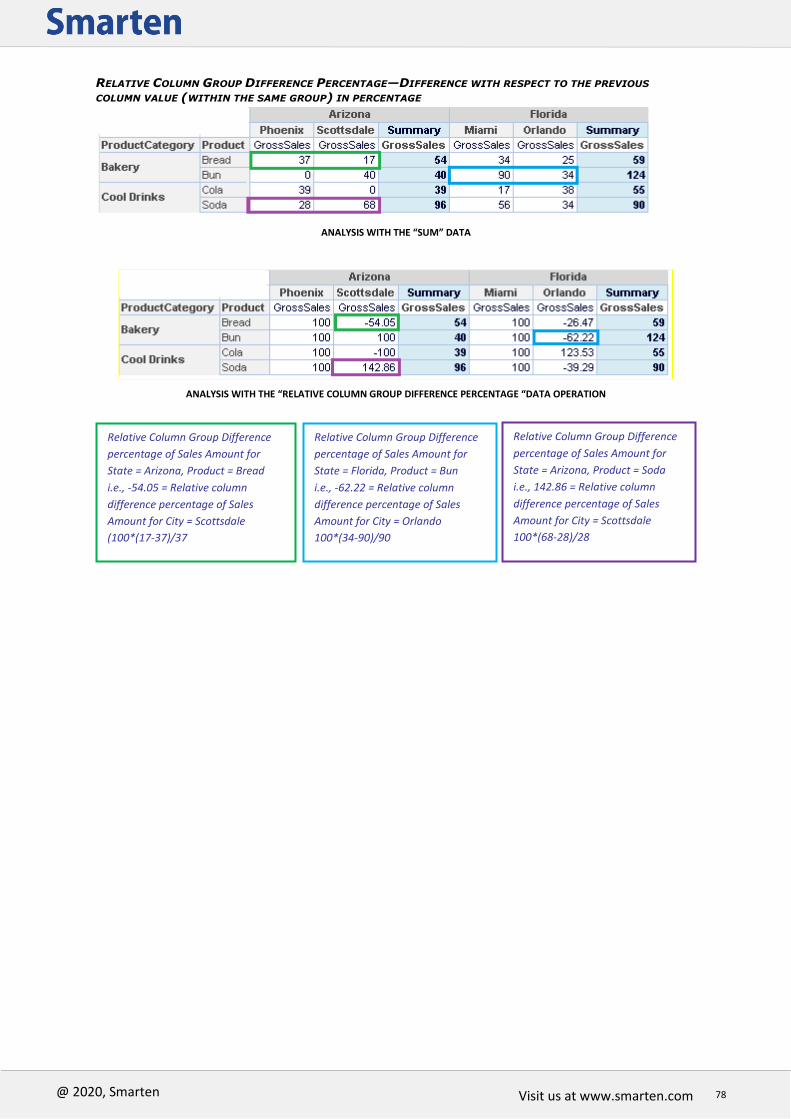
Visit us at www.smarten.com 78
@ 2020, Smarten
Visit us at
RELATIVE COLUMN GROUP DIFFERENCE PERCENTAGE—DIFFERENCE WITH RESPECT TO THE PREVIOUS
COLUMN VALUE (WITHIN THE SAME GROUP) IN PERCENTAGE
ANALYSIS WITH THE “SUM” DATA
ANALYSIS WITH THE “RELATIVE COLUMN GROUP DIFFERENCE PERCENTAGE “DATA OPERATION
Relative Column Group Difference
percentage of Sales Amount for
State = Arizona, Product = Bread
i.e., -54.05 = Relative column
difference percentage of Sales
Amount for City = Scottsdale
(100*(17-37)/37
Relative Column Group Difference
percentage of Sales Amount for
State = Arizona, Product = Soda
i.e., 142.86 = Relative column
difference percentage of Sales
Amount for City = Scottsdale
100*(68-28)/28
Relative Column Group Difference
percentage of Sales Amount for
State = Florida, Product = Bun
i.e., -62.22 = Relative column
difference percentage of Sales
Amount for City = Orlando
100*(34-90)/90

Visit us at www.smarten.com 79
@ 2020, Smarten
Visit us at
Row Cumulative Sum—Row wise cumulative sum of all previous values for every column
ANALYSIS WITH THE “SUM” DATA
ANALYSIS WITH THE “ROW CUMULATIVE SUM” DATA OPERATION
Row Cumulative Sum of Sales Amount for
State = Arizona
City = Phoenix
Product = Bread is 37{37+0}
Product = Bun is 37{0+37}
Product = Cola is 76{39+37}
Product = Soda is 104{28+76}
Row Cumulative Sum of Sales Amount for
State = Florida
City = Miami
Product = Bread is 34{34+0}
Product = Bun is 124{90+34}
Product = Cola is 141{17+124}
Product = Soda is 197{56+141}

Visit us at www.smarten.com 80
@ 2020, Smarten
Visit us at
Row Group Cumulative Sum—Row wise cumulative sum of all previous values for every
column (within the same group)
ANALYSIS WITH THE “SUM” DATA
ANALYSIS WITH THE “ROW GROUP CUMULATIVE SUM” DATA
Row Group cumulative sum of Sales Amount for
City = Phoenix
Product = Bun
i.e., 37 = Row cumulative sum of Sales Amount (37+0)
Row Group cumulative sum of Sales Amount for
City = Miami
Product = Soda
i.e., 72 = Row cumulative sum of Sales Amount (38+34)

Visit us at www.smarten.com 81
@ 2020, Smarten
Visit us at
Column Cumulative Sum—Column wise cumulative sum of all previous values for every
row
ANALYSIS WITH THE “SUM” DATA
ANALYSIS WITH THE “COLUMN CUMULATIVE SUM” DATA
Column Cumulative Sum of Sales Amount for
State = Arizona and Florida
Product = Bread
City = Phoenix is 37{37+0}
City = Scottsdale is 54{17+37}
City = Miami is 88{34+54}
City = Orlando is 113{25+88}
Column Cumulative Sum of Sales Amount for
State = Arizona and Florida
Product = Cola
City = Phoenix is 39{39+0}
City = Scottsdale is 39{0+39}
City = Miami is 56{17+39}
City = Orlando is 94{38+56}

Visit us at www.smarten.com 82
@ 2020, Smarten
Visit us at
Column Group Cumulative Sum—Column wise cumulative sum of all previous values for
every row (within the same group)
ANALYSIS WITH THE “SUM” DATA
ANALYSIS WITH THE “COLUMN GROUP CUMULATIVE SUM” DATA
Column Group cumulative sum of Sales Amount for
City = Scottsdale
Product = Bread
i.e., 54 = Column cumulative sum of Sales Amount for the
group Arizona (37+17)
Column Group cumulative sum of Sales Amount for
City = Orlando
Product = Bun
i.e., 124 = Column cumulative sum of Sales Amount for
the group Florida (90+34)

Visit us at www.smarten.com 83
@ 2020, Smarten
Visit us at
Distinct Count – Unique (Distinct) count value of specified dimension
Transaction id State City Product Category Product Gross Sales
A1 Florida Miami Bakery Bread 34
A2 Florida Miami Bakery Bun 46
A3 Florida Miami Cool Drinks Cola 17
A4 Florida Miami Cool Drinks Soda 56
A5 Florida Miami Bakery Bun 44
A6 Florida Orlando Bakery Bread 25
A7 Florida Orlando Bakery Bun 34
A8 Florida Orlando Cool Drinks Cola NULL
A9 Florida Orlando CoolDrinks Soda NULL
A10 Florida Orlando CoolDrinks Cola 38
A11 Florida Orlando Cool Drinks Soda 34
A12 Arizona Phoenix Bakery Bread 12
A13 Arizona Phoenix Bakery Bun NULL
A14 Arizona Phoenix Cool Drinks Cola 39
A15 Arizona Phoenix Cool Drinks Soda 28
A16 Arizona Phoenix Bakery Bread 25
A17 Arizona Scottsdale Bakery Bread 17
A18 Arizona Scottsdale Bakery Bun 6
A19 Arizona Scottsdale Cool Drinks Cola NULL
A20 Arizona Scottsdale Cool Drinks Soda 68
A21 Arizona Scottsdale Bakery Bun 34
A22 Arizona Scottsdale Bakery Cookies 20
ANALYSIS WITH THE “SUM” DATA
.
ANALYSIS WITH “DISTINCT COUNT” ON PRODUCT—PRODUCT CATEGORY-WISE – STATE-WISE
3 = Distinct Count of Product for
State = Arizona
Product Category =Bakery
(Bread, Bun, and Cookies are distinct Products)
2 = Distinct Count of Product for
State = Florida
Product Category = Cool Drinks
(Cola and Soda are two distinct Products)

Visit us at www.smarten.com 84
@ 2020, Smarten
Visit us at
Distinct Sum and Distinct Average –Sum and Average of Unique (Distinct) value of a specified dimension
Sales Date Year State Product Target (Yearly) Actual Sales
1-Jan-2015 2015 Arizona Bakery 250000 25000
10-Jan-2015 2015 Arizona Tea 200000 30000
15-Feb-2015 2015 Arizona Bakery 250000 45000
16-Feb-2015 2015 Arizona Tea 200000 22500
15-Apr-2015 2015 Arizona Bakery 250000 50000
16-May-2015 2015 Arizona Tea 200000 35000
12-Jun-2015 2015 Arizona Bakery 250000 43000
11-Jul-2015 2015 Arizona Tea 200000 35500
17-Aug-2015 2015 Arizona Bakery 250000 56500
9-Sep-2015 2015 Arizona Tea 200000 42000
12-Nov-2015 2015 Arizona Bakery 250000 51500
15-Dec-2015 2015 Arizona Tea 200000 40000
12-Jan-2016 2016 Arizona Bakery 300000 30000
15-Jan-2016 2016 Arizona Tea 250000 35000
14-Feb-2016 2016 Arizona Bakery 300000 35000
20-Feb-2016 2016 Arizona Tea 250000 29000
13-Mar-2016 2016 Arizona Bakery 300000 38000
5-Apr-2016 2016 Arizona Tea 250000 29500
15-May-2016 2016 Arizona Bakery 300000 35000
15-Jun-2016 2016 Arizona Tea 250000 32000
8-Jul-2016 2016 Arizona Bakery 300000 30000
16-Jul-2016 2016 Arizona Tea 250000 30000
20-Aug-2016 2016 Arizona Bakery 300000 32000
5-Sep-2016 2016 Arizona Tea 250000 35000
12-Oct-2016 2016 Arizona Bakery 300000 40000
15-Nov-2016 2016 Arizona Tea 250000 32000
ANALYSIS WITH THE “SUM” DATA

Visit us at www.smarten.com 85
@ 2020, Smarten
Visit us at
ANALYSIS WITH “DISTINCT SUM” OF “TARGET” FOR DISTINCT COLUMN “YEAR”
ANALYSIS WITH “DISTINCT AVERAGE” OF “TARGET” FOR DISTINCT COLUMN “YEAR”
Most Recent and Least Recent Functions
Applying this function returns the result of different aggregation methods on the most recent or least recent records from the data, based on the date dimension. For analysis of data that is recorded over a period of time, aggregation-related data operations of values may not be important, but most recent and least recent values can be important. Certain data values change frequently and recorded as closing balance or aggregated balance to date. This closing balance or aggregated values need to be analysed from time to time, as these changed values can affect the trends over a particular time span. So it becomes important to know the most recent or least recent data values to measure change in the trends. Consider a scenario where year-to-date Gross Sales is recorded at the end of every month, which represents total sales from beginning of the year till end of that particular month. For example, if year is beginning from January, then sales recorded in February is sales from January to February, and sales recorded in June is the sales from January to June.
275000= Distinct Average of “Year” for
Product = Bakery
(250000 (2015) + 300000 (2016) / 2 = 275000 is
Distinct Average)

Visit us at www.smarten.com 86
@ 2020, Smarten
Visit us at
YTD SALES DATA—MONTHLY VIEW
On applying Quarterly view on this data, the YTD Most Recent Gross Sales for March, June, and July would be shown as below.
MOST RECENT VALUES—QUARTERLY VIEW
Similarly, on applying Quarterly view on this data, the YTD Least Recent Gross Sales for March, June, and July would be shown as below.
LEAST RECENT VALUES—QUARTERLY VIEW
Example data set for all examples in this section:
Transaction ID
State City Product Category
Product Date (MM/DD/YYYY)
Gross Sales
A1 Arizona Phoenix Bakery Bread 1/2/2014 12
A2 Arizona Phoenix Bakery Bread 1/23/2014 25
A3 Arizona Phoenix Bakery Bun 1/4/2014 0
A4 Arizona Phoenix Cool Drinks Cola 1/8/2014 39
A5 Arizona Phoenix Cool Drinks Soda 1/28/2014 55
A6 Arizona Phoenix Cool Drinks Soda 1/3/2014 28
A7 Arizona Scottsdale Bakery Bread 1/19/2014 17
A8 Arizona Scottsdale Bakery Bread 1/23/2014 20
A9 Arizona Scottsdale Bakery Bun 1/12/2014 6
A10 Arizona Scottsdale Bakery Bread 1/2/2014 35
A11 Arizona Scottsdale Bakery Bun 1/13/2014 34
A12 Arizona Scottsdale Cool Drinks Cola 1/2/2014 45
A13 Arizona Scottsdale Cool Drinks Cola 1/17/2014 0
A14 Arizona Scottsdale Cool Drinks Soda 1/28/2014 68
A15 Florida Miami Bakery Bread 1/6/2014 34

Visit us at www.smarten.com 87
@ 2020, Smarten
Visit us at
A16 Florida Miami Bakery Bread 1/2/2014 20
A17 Florida Miami Bakery Bread 1/23/2014 30
A18 Florida Miami Bakery Bun 1/13/2014 45
A19 Florida Miami Bakery Bun 1/17/2014 44
A20 Florida Miami Cool Drinks Cola 1/2/2014 40
A21 Florida Miami Cool Drinks Soda 1/28/2014 50
A22 Florida Miami Cool Drinks Cola 1/11/2014 17
A23 Florida Miami Cool Drinks Soda 1/25/2014 56
A24 Florida Orlando Bakery Bread 1/7/2014 25
A25 Florida Orlando Bakery Bread 1/2/2014 15
A26 Florida Orlando Bakery Bread 1/23/2014 18
A27 Florida Orlando Bakery Bun 1/18/2014 34
A28 Florida Orlando CoolDrinks Cola 1/2/2014 0
A29 Florida Orlando Cool Drinks Cola 1/19/2014 38
A30 Florida Orlando Cool Drinks Soda 1/28/2014 60
A31 Florida Orlando Cool Drinks Soda 1/15/2014 34
A32 Florida Orlando Cool Drinks Soda 1/21/2014 0
ORIGINAL ANALYSIS WITH THE “SUM” DATA AT THE ROW LEVEL

Visit us at www.smarten.com 88
@ 2020, Smarten
Visit us at
Most Recent values:
In the following examples, the displayed values are the Most Recent Values for the month of January.
ANALYSIS WITH THE “MOST RECENT” FUNCTION ON THE DATA
AT THE LEVEL OF “PRODUCTCATEGORY” AND “STATE” DIMENSIONS
ANALYSIS WITH THE “MOST RECENT” FUNCTION ON THE DATA
AT THE LEVEL OF “PRODUCTCATEGORY” AND “CITY” DIMENSIONS
ANALYSIS WITH THE “MOST RECENT” FUNCTION ON THE DATA
AT THE LEVEL OF “PRODUCT” AND “CITY” DIMENSIONS
20 = The Most Recent value for
State = Arizona
Product Category = Bakery
Date = 23-Jan {A8}
60 = The Most Recent value for
State = Florida
Product Category = Cool Drinks
Date = 28-Jan {A30}
25 = The Most Recent value for
State = Arizona
City = Phoenix
Product Category = Bakery
Date = 23-Jan {A2}
20 = The Most Recent value for
State = Arizona
City = Scottsdale
Product Category = Bakery
Date = -23-Jan {A8}
60 = The Most Recent value for State
= Florida
City = Orlando
Product Category = Cool Drinks
Date = -28-Jan {A30}

Visit us at www.smarten.com 89
@ 2020, Smarten
Visit us at
Least Recent values:
In the following example, the displayed values are the Least Recent Values for the month of January.
ANALYSIS WITH THE “LEAST RECENT” FUNCTION ON THE DATA
AT THE LEVEL OF “PRODUCTCATEGORY” AND “STATE” DIMENSIONS
ANALYSIS WITH THE “LEAST RECENT” FUNCTION ON THE DATA
AT THE LEVEL OF “PRODUCTCATEGORY” AND “CITY” DIMENSIONS
ANALYSIS WITH THE “LEAST RECENT” FUNCTION ON THE DATA
AT THE LEVEL OF “PRODUCT” AND “CITY” DIMENSIONS
12 = The Least Recent value (the earliest entry) for State
= Arizona
Product Category = Bakery
Date = -2-Jan {A1}
45= The Least Recent value for
State = Arizona
Product Category = Cool Drinks
Date = -2-Jan {A12}
12 = The Least Recent value for
State = Arizona
City = Phoenix
Product Category = Bakery
Date = 2-Jan {A1}
35 = The Most Recent value for
State = Arizona
City = Scottsdale
Product Category = Bakery
Date = 2-Jan {A10}
40 = The Most Recent value for
State = Florida
City = Miami
Product Category = Cool Drinks
Date = 2-Jan {A20}
12 = The Least Recent value for
State = Arizona
City = Phoenix
Product Category = Bakery Product
= Bread
Date = 2-Jan {A1}
35 = The Least Recent value for
State = Arizona
City = Scottsdale
Product Category = Bakery
Product = Bread
Date = 2-Jan {A10}
6 = The Most Recent value for
State = Arizona
City = Scottsdale
Product Category = Bakery
Product = Bun
Date = 12-Jan {A9}

Visit us at www.smarten.com 90
@ 2020, Smarten
Visit us at
MOST RECENT AND LEAST RECENT WITH AGGREGATION FUNCTIONS:
If multiple records are found on the least recent or most recent date dimension, user can apply aggregation function on these records. For example, if January 28 is the most recent date available for January and there are 5 transactions available on this date, user can choose aggregation function to be applied on these records. If no aggregation function is selected, system will show the least or most recent record that is retrieved from the data. Different Aggregated functions used on Most Recent and Least Recent Operations are as follows:
Aggregated Function
Description
None In case of Least Recent, this shows the first transaction for the recent date.
In case of Most Recent, this shows the last transaction for the recent date.
Sum Sum of all the least or most recent date transactions
Average Average of all the least or most recent date transactions
Minimum Minimum value of the least or most recent date transactions
Maximum Maximum value of the least or most recent date transactions
Effective Average Average (excluding NULL transactions) of the least or most recent date transactions
Count Total number of least or most recent date transactions
Effective Count Count of Total number of least or most recent date transactions (excluding NULL transactions)
Most Recent: With Aggregation Functions
ANALYSIS WITH THE “MOST RECENT” FUNCTION ON THE DATA USING “AVERAGE”
AGGREGATION METHOD AT THE LEVEL OF “PRODUCTCATEGORY” AND “STATE” DIMENSIONS
22.5 = Most Recent value using Average Aggregation
Function for
State = Arizona;
Product Category = Bakery
Date =23-Jan {(A2+A8)/2}
55=Most Recent value using Average Aggregation
Function for
State = Florida
Product Category = Cool Drinks
Date =28-Jan {(A21+A30)/2}

Visit us at www.smarten.com 91
@ 2020, Smarten
Visit us at
LEAST RECENT: WITH AGGREGATION FUNCTIONS
ANALYSIS WITH THE “LEAST RECENT” FUNCTION ON THE DATA USING “AVERAGE”
AGGREGATION METHOD AT THE LEVEL OF “PRODUCTCATEGORY” AND “STATE” DIMENSIONS
Post Aggregation on Most Recent and Least Recent: After applying Most Recent and Least Recent operation, user can also apply post aggregation data operation. Post aggregation data operation will be applied on values derived after applying most recent or least recent function at the front-end object level data. The following post aggregation data operations can be applied:
Post Aggregation Function Description
None No effect
Row Percentage Percentage value against row level summary within the same row (after applying most recent or least recent operation)
Row Group Percentage Percentage value against the row group level summary (within the same group)(after applying most recent or least recent operation)
Column Percentage Percentage value against column level summary within the same column (after applying most recent or least recent operation)
Column Group Percentage Percentage value against the column group level summary (within the same group) (after applying most recent or least recent operation)
Total Percentage Percentage value against the total crosstab sum (after applying most recent or least recent operation)
Relative Row Group Difference
Difference with respect to the previous row value (within same group) (after applying most recent or least recent operation)
Relative Row Group Difference Percentage
Difference with respect to the previous row value (within same group) in percentage (after applying most recent or least recent operation)
Relative Column Group Difference
Difference with respect to the previous column value (within the same group) (after applying most recent or least recent operation)
Relative Column Group Difference Percentage
Difference with respect to the previous column value (within the same group) in percentage (after applying most recent or least recent operation)
Row Group Cumulative Sum
Row wise cumulative sum of all previous values for every column (within the same group) (after applying most recent or least recent operation)
Column Group Cumulative Sum
Column wise cumulative sum of all previous values for every row (within the same group) (after applying most recent or least recent operation)
MOST RECENT: WITH POST AGGREGATION FUNCTION
23.5 = Least Recent value using Average Aggregation
Function for
State = Arizona
Product Category = Bakery
Date = 2-Jan {(A1+A10)/2}
20 = Least Recent value using Average Aggregation
Function for
State = Florida
Product Category = Cool Drinks
Date = 2-Jan {(A20+A28)/2}

Visit us at www.smarten.com 92
@ 2020, Smarten
Visit us at
ANALYSIS WITH THE “MOST RECENT” FUNCTION ON THE DATA USING “AVERAGE”
AGGREGATION METHOD AT THE LEVEL OF “PRODUCTCATEGORY” AND “STATE” DIMENSIONS
ANALYSIS WITH THE “MOST RECENT” FUNCTION ON THE DATA USING “AVERAGE”
AGGREGATION METHOD AT THE LEVEL OF “PRODUCTCATEGORY” AND “STATE” DIMENSIONS WITH “ROW PERCENTAGE” POST
AGGREGATION FUNCTION
48.39 = Most Recent Function using Row Percentage
Post Aggregation Function on Average Aggregation
Function
For State = Arizona
Product Category = Bakery
{(22.5/ (22.5+24))*100}
47.21 = Most Recent Function using Row Percentage
Post Aggregation Function on Average Aggregation
Function
For State = Florida
Product Category = Cool Drinks
{(55/ (61.5+55))*100}

Visit us at www.smarten.com 93
@ 2020, Smarten
Visit us at
LEAST RECENT: WITH POST AGGREGATION FUNCTION
ANALYSIS WITH THE “LEAST RECENT” FUNCTION ON THE DATA USING “AVERAGE”
AGGREGATION METHOD AT THE LEVEL OF “PRODUCTCATEGORY” AND “STATE” DIMENSIONS
ANALYSIS WITH THE “LEAST RECENT” FUNCTION ON THE DATA USING “AVERAGE”
AGGREGATION METHOD AT THE LEVEL OF “PRODUCTCATEGORY” AND “STATE” DIMENSIONS
WITH “ROW PERCENTAGE” POST AGGREGATION FUNCTION
57.32 = Least Recent Function using Row Percentage Post
Aggregation Function on Average Aggregation Function
For State = Arizona
Product Category = Bakery
{(23.5/ (23.5+17.5))/100}
30.77 = Least Recent Function using Row Percentage
Post Aggregation Function on Average Aggregation
Function
For State = Florida
Product Category = Cool Drinks
{(20/ (45+20))/100}

Visit us at www.smarten.com 94
@ 2020, Smarten
Visit us at
4.12 Summary Operations
Multilevel Summary Operations The user can define various summary operations at row and column level. Example data set for all examples in this section:
Transaction id State City Product Category
Product Gross Sales
A1 Florida Miami Bakery Bread 34
A2 Florida Miami Bakery Bun 46
A3 Florida Miami Cool Drinks Cola 17
A4 Florida Miami Cool Drinks Soda 56
A5 Florida Miami Bakery Bun 44
A6 Florida Orlando Bakery Bread 25
A7 Florida Orlando Bakery Bun 34
A8 Florida Orlando Cool Drinks Cola <NULL>
A9 Florida Orlando CoolDrinks Soda <NULL>
A10 Florida Orlando CoolDrinks Cola 38
A11 Florida Orlando Cool Drinks Soda 34
A12 Arizona Phoenix Bakery Bread 12
A13 Arizona Phoenix Bakery Bun <NULL>
A14 Arizona Phoenix Cool Drinks Cola 39
A15 Arizona Phoenix Cool Drinks Soda 28
A16 Arizona Phoenix Bakery Bread 25
A17 Arizona Scottsdale Bakery Bread 17
A18 Arizona Scottsdale Bakery Bun 6
A19 Arizona Scottsdale Cool Drinks Cola <NULL>
A20 Arizona Scottsdale Cool Drinks Soda 68
A21 Arizona Scottsdale Bakery Bun 34
Various summaries that can be added up to the nth level in the analysis.
SUMMARY AT ROW AND COLUMN LEVEL
MULTILEVEL ROW SUMMARIES

Visit us at www.smarten.com 95
@ 2020, Smarten
Visit us at
MULTILEVEL COLUMN SUMMARIES

Visit us at www.smarten.com 96
@ 2020, Smarten
Visit us at
List of Summary Operations:
1. Sum
Applied on cube row level data.
2. Average
3. Effective Average
4. Count
5. Effective Count
6. Maximum
7. Minimum
8. First
9. Last
10. Default
Applied on the front-end object view data.
11. Group Sum
12. Group Average
13. Group Count
14. Group Maximum
15. Group Minimum
16. Row Percentage
17. Row Group Percentage
18. Column Percentage
19. Column Group Percentage
20. Total Percentage
21. Relative Row Difference
22. Relative Row Difference Percentage
23. Relative Row Group Difference
24. Relative Row Group Difference Percentage
25. Relative Column Difference
26. Relative Column Difference Percentage
27. Relative Column Group Difference
28. Relative Column Group Difference Percentage
29. Row Cumulative Sum
30. Row Group Cumulative Sum
31. ColumnCumulative Sum
32. Column Group Cumulative Sum
Row / Column Summary Summary operations described below with examples.
ANALYSIS WITH THE “SUM” DATA OPERATION

Visit us at www.smarten.com 97
@ 2020, Smarten
Visit us at
DEFAULT—DEFAULT SUMMARY OPERATION WILL APPLY SUMMARY BASED ON DATA OPERATION APPLIED ON
THE COLUMNS.
ANALYSIS WITH THE “AVERAGE” DATA OPERATION
ANALYSIS WITH THE “DEFAULT” SUMMARY OPERATION
Sum—Sum of all values
ANALYSIS WITH THE “SUM” SUMMARY OPERATION
Group Sum—Total/Sum of all values across a row or column at group level
ANALYSIS WITH THE “MAXIMUM” DATA OPERATION AND “DEFAULT” SUMMARY OPERATION

Visit us at www.smarten.com 98
@ 2020, Smarten
Visit us at
ANALYSIS WITH THE “MAXIMUM” DATA OPERATION AND “GROUP SUM” SUMMARY OPERATION
AVERAGE—AVERAGE OF ALL VALUES
ANALYSIS WITH THE “AVERAGE” SUMMARY OPERATION
EFFECTIVE AVERAGE—AVERAGE OF ALL ―NOT NULL‖ VALUES
Note:
Effective Average implies the average of only the rows with “not null” values. Columns with
value “null” are not considered in effective average calculation, but columns with value “0”
are taken into consideration for effective average calculation.
ANALYSIS WITH THE “EFFECTIVE AVERAGE” SUMMARY OPERATION

Visit us at www.smarten.com 99
@ 2020, Smarten
Visit us at
GROUP AVERAGE—AVERAGE OF ALL VALUES WITHIN THE SAME GROUP
ANALYSIS WITH THE “SUM” SUMMARY OPERATION
ANALYSIS WITH THE “GROUP AVERAGE” SUMMARY OPERATION
COUNT—COUNT OF ALL VALUES
ANALYSIS WITH THE “COUNT” SUMMARY OPERATION

Visit us at www.smarten.com 100
@ 2020, Smarten
Visit us at
EFFECTIVE COUNT—COUNT OF ALL ―NOT NULL‖ VALUES
Note:
Effective Count implies the count of only the rows with “not null” values. Columns with value
“null” are not considered in effective count calculation, but a column with value “0” is taken
into consideration for effective count calculation.
ANALYSIS WITH THE “EFFECTIVE COUNT” SUMMARY OPERATION
GROUP COUNT—COUNT OF ALL VALUES WITHIN THE SAME GROUP
ANALYSIS WITH THE “GROUP COUNT” SUMMARY OPERATION
MAXIMUM—HIGHEST AMONG ALL THE VALUES
ANALYSIS WITH THE “MAXIMUM” SUMMARY OPERATION

Visit us at www.smarten.com 101
@ 2020, Smarten
Visit us at
GROUP MAXIMUM—HIGHEST AMONG ALL THE VALUES WITHIN THE SAME GROUP
ANALYSIS WITH THE “GROUP MAXIMUM” SUMMARY OPERATION
MINIMUM—LOWEST AMONG ALL THE VALUES
ANALYSIS WITH THE “MINIMUM” SUMMARY OPERATION
GROUP MINIMUM—LOWEST AMONG ALL THE VALUES WITHIN THE SAME GROUP
ANALYSIS WITH THE “GROUP MINIMUM” SUMMARY OPERATION
FIRST—FIRST AMONG ALL THE VALUES
ANALYSIS WITH THE “FIRST” SUMMARY OPERATION

Visit us at www.smarten.com 102
@ 2020, Smarten
Visit us at
LAST—LAST AMONG ALL THE VALUES
ANALYSIS WITH THE “LAST” SUMMARY OPERATION
ROW PERCENTAGE—SUMMARY PERCENTAGE VALUE AGAINST ROW LEVEL SUMMARY
ANALYSIS WITH THE “SUM” DATA
ANALYSIS WITH THE “ROW PERCENTAGE” SUMMARY OPERATION
ROW GROUP PERCENTAGE—GROUP SUMMARY PERCENTAGE VALUE AGAINST ROW LEVEL SUMMARY (WITHIN
SAME GROUP)
ANALYSIS WITH THE “SUM” DATA

Visit us at www.smarten.com 103
@ 2020, Smarten
Visit us at
ANALYSIS WITH THE “ROW GROUP PERCENTAGE” SUMMARY OPERATION
TOTAL PERCENTAGE—SUMMARY PERCENTAGE VALUE AGAINST TOTAL CROSSTAB SUM
ANALYSIS WITH THE “SUM” DATA
ANALYSIS WITH THE “TOTAL PERCENTAGE” SUMMARY OPERATION
RELATIVE ROW DIFFERENCE—DIFFERENCE WITH RESPECT TO THE PREVIOUS SUMMARY ROW
ANALYSIS WITH THE “SUM” DATA

Visit us at www.smarten.com 104
@ 2020, Smarten
Visit us at
ANALYSIS WITH THE “RELATIVE ROW DIFFERENCE” SUMMARY OPERATION
RELATIVE ROW DIFFERENCE PERCENTAGE—DIFFERENCE WITH RESPECT TO THE PREVIOUS SUMMARY ROW IN
PERCENTAGE
ANALYSIS WITH THE “SUM” DATA

Visit us at www.smarten.com 105
@ 2020, Smarten
Visit us at
ANALYSIS WITH THE “RELATIVE ROW DIFFERENCE PERCENTAGE” SUMMARY OPERATION
RELATIVE ROW GROUP DIFFERENCE—DIFFERENCE WITH RESPECT TO THE PREVIOUS SUMMARY ROW FOR
RESPECTIVE GROUP
ANALYSIS WITH THE ”SUM” DATA

Visit us at www.smarten.com 106
@ 2020, Smarten
Visit us at
ANALYSIS WITH THE “RELATIVE ROW GROUP DIFFERENCE” SUMMARY OPERATION
RELATIVE ROW GROUP DIFFERENCE PERCENTAGE—DIFFERENCE WITH RESPECT TO THE PREVIOUS SUMMARY
ROW IN PERCENTAGE FOR RESPECTIVE GROUP
ANALYSIS WITH THE “SUM” DATA
ANALYSIS WITH THE “RELATIVE ROW GROUP DIFFERENCE PERCENTAGE” SUMMARY OPERATION

Visit us at www.smarten.com 107
@ 2020, Smarten
Visit us at
COLUMN PERCENTAGE—SUMMARY PERCENTAGE VALUE AGAINST COLUMN LEVEL SUMMARY WITHIN THE SAME
COLUMN
ANALYSIS WITH THE “SUM” DATA
ANALYSIS WITH THE “COLUMN PERCENTAGE” SUMMARY OPERATION
COLUMN GROUP PERCENTAGE—GROUP SUMMARY PERCENTAGE VALUE AGAINST COLUMN LEVEL SUMMARY
(WITHIN SAME GROUP)
ANALYSIS WITH THE “SUM” DATA
ANALYSIS WITH THE “COLUMN GROUP PERCENTAGE” FUNCTION APPLIED ON SUMMARY OPERATION

Visit us at www.smarten.com 108
@ 2020, Smarten
Visit us at
RELATIVE COLUMN DIFFERENCE—DIFFERENCE WITH RESPECT TO THE PREVIOUS SUMMARY COLUMN
ANALYSIS WITH THE “SUM” DATA
ANALYSIS WITH THE “RELATIVE COLUMN DIFFERENCE” SUMMARY OPERATION
RELATIVE COLUMN DIFFERENCE PERCENTAGE—DIFFERENCE WITH RESPECT TO THE PREVIOUS SUMMARY
COLUMN IN PERCENTAGE
ANALYSIS WITH THE “SUM” DATA
ANALYSIS WITH THE “RELATIVE COLUMN DIFFERENCE PERCENTAGE” SUMMARY OPERATION

Visit us at www.smarten.com 109
@ 2020, Smarten
Visit us at
RELATIVE COLUMN GROUP DIFFERENCE—DIFFERENCE WITH RESPECT TO THE PREVIOUS SUMMARY COLUMN
FOR PARTICULAR GROUP
ANALYSIS WITH THE “SUM” DATA
ANALYSIS WITH THE “RELATIVE COLUMN GROUP DIFFERENCE” SUMMARY OPERATION
RELATIVE COLUMN GROUP DIFFERENCE PERCENTAGE—DIFFERENCE WITH RESPECT TO THE PREVIOUS
SUMMARY COLUMN IN PERCENTAGE FOR PARTICULAR GROUP
ANALYSIS WITH THE “SUM” DATA
ANALYSIS WITH THE “RELATIVE COLUMN GROUP DIFFERENCE PERCENTAGE” SUMMARY OPERATION

Visit us at www.smarten.com 110
@ 2020, Smarten
Visit us at
ROW CUMULATIVE SUM—CUMULATIVE SUM OF ALL PREVIOUS ROW SUMMARIES IN THE SAME ROW
ANALYSIS WITH THE “SUM” DATA
ANALYSIS WITH THE “ROW CUMULATIVE SUM” SUMMARY OPERATION
ROW GROUP CUMULATIVE SUM—CUMULATIVE SUM OF ALL PREVIOUS ROW SUMMARIES IN THE SAME GROUP
ANALYSIS WITH THE “SUM” DATA

Visit us at www.smarten.com 111
@ 2020, Smarten
Visit us at
ANALYSIS WITH THE “ROW GROUP CUMULATIVE SUM” SUMMARY OPERATION
COLUMN CUMULATIVE SUM—CUMULATIVE SUM OF ALL PREVIOUS COLUMN SUMMARIES IN THE SAME COLUMN
ANALYSIS WITH THE “SUM” DATA
ANALYSIS WITH THE “COLUMN CUMULATIVE SUM” SUMMARY OPERATION
COLUMN GROUP CUMULATIVE SUM—CUMULATIVE SUM OF ALL PREVIOUS COLUMN SUMMARIES IN THE SAME
COLUMN
ANALYSIS WITH THE “SUM” DATA
ANALYSIS WITH THE “COLUMN GROUP CUMULATIVE SUM” SUMMARY OPERATION

Visit us at www.smarten.com 112
@ 2020, Smarten
Visit us at
OPTION TO CALCULATE SUMMARY USING CHILD LEVEL SUMMARY DATA
In earlier versions, users were able to apply a summary based on various back-end and front-end
summary operations. In this version, Smarten provides a new option to calculate a summary based
on a child level summary.
For example, there is one crosstab with 2 row dimensions: ProductCategory and ProductName and
one measure GrossSales with sum data operation. On the ProductName column, a summary is
applied with the count summary operation. Now, if the user wants to see the sum of count values of
the Productname summary in the Productcategory summary, the user needs to select “calculate
summary on child level summary” check box while applying the summary on the ProductCategory
column. The system will calculate the summary using the Productname summary data.
CALCULATE SUMMARY USING CHILD SUMMARY
CALCULATE SUMMARY USING CHILD SUMMARY SETTING

Visit us at www.smarten.com 113
@ 2020, Smarten
Visit us at
4.13 Trend Line
Trend lines are used to determine trends and movement of trends, which is also called regression analysis. A trend line is created when user draws a diagonal line between two or more points in a chart. When establishing trend lines, it is important to choose a chart based on time intervals. The time interval in the chart can be hourly, daily, weekly, monthly, quarterly, and yearly periods.
GRAPHIC ANALYSIS WITH TREND LINES
Types of trend lines
Linear
Logarithmic
Polynomial
Power
Exponential
Moving Average
Note:
Trend Lines cannot be applied to stacked and percentage graphs.

Visit us at www.smarten.com 114
@ 2020, Smarten
Visit us at
4.13.1 Linear Trend line
If data values are going up or down at a steady rate, a linear trend line is best to depict its nature. A linear trend line usually shows that something is increasing or decreasing at a steady rate. Example: As per the increase in a state’s population, consumption of products increases
EXAMPLE OF A LINEAR TREND LINE FOR ALCOHOLIC DRINKS
How does linear trend line compute? A linear trend line is drawn by using the following equation to calculate the least squares fit for a line:
y = mx + b where m is the slope and b is the intercept. Guidelines:
With linear data patterns, i.e., data points resembling a line either increasing or decreasing at a steady rate (simple linear data sets), a linear trend line should be applied
A linear trend line will not adjust to any changes in the trend

Visit us at www.smarten.com 115
@ 2020, Smarten
Visit us at
4.13.2 Logarithmic Trend line
A logarithmic trend line is a best-fit curved line that is most useful when the rate of change in the data increases or decreases quickly and then levels out. A logarithmic trend line can use negative and/or positive values. Example: Population growth in a region increases or decreases periodically
EXAMPLE OF A LOGARITHMIC TREND LINE FOR ALCOHOLIC DRINKS
How does logarithmic trend line compute? A logarithmic trend line is drawn by using the following equation to calculate the least squares fit through points:
y = cln x + b where c and b are constants, and ln is the natural logarithm function.
Guidelines:
With data points having a relative sharp curve at one end and then gradually levels out, logarithmic trend line should be applied
Logarithmic trend line tends to hide accelerating trends in the short/medium run. In accelerating trends where no steady growth rate is possible, the logarithmic trend line should not to be used

Visit us at www.smarten.com 116
@ 2020, Smarten
Visit us at
4.13.3 Polynomial Trend line
A polynomial trend line is a curved line that is used when data fluctuates in a rhythmic manner. It is useful, for example, for analyzing gains and losses over a large data set. The order of the polynomial can be determined by the number of fluctuations in the data or by how many bends (ups and downs) appear in the curve. An Order 2 polynomial trend line generally has only one up or down. Order 3 generally has one or two ups or downs, and similarly order 4 generally has up to three ups or downs and so on. Example: Sale of seasonal fruits in the past 10 years
EXAMPLE OF A POLYNOMIAL TREND LINE FOR ALCOHOLIC DRINKS
How does polynomial trend line compute? A polynomial or curvilinear trend line is drawn by using the following equation to calculate the least squares fit through points:
y = b + c1x + c2x2 + c3x
3+ . . . + c6x
6
where b and c1,c2,.....,c6 are constants.
Guidelines:
A polynomial trend line is a curved line that is used when data fluctuates. Based on the number of fluctuations, the order of a polynomial trend line can be decided
A polynomial trend line fitted throughout a long data series will be incapable of revealing short-term market fluctuations, such as seasonal patterns

Visit us at www.smarten.com 117
@ 2020, Smarten
Visit us at
4.13.4 Power Trend line
If the graph data changes at a steadily increasing or decreasing rate as in an acceleration curve, a power trend line is a curved line that is best used. You cannot create a power trend line if your data contains zero or negative values. Example: The acceleration of a racing car for the first 20-second interval
EXAMPLE OF A POWER TREND LINE FOR ALCOHOLIC DRINKS
How does power trend line compute? A power trend line by using the following equation to calculate the least squares fit through points:
y = cxb
where c and b are constants.
Note:
This option is not available when your data includes negative or zero values.
Guidelines:
Very practical for acceleration or deceleration graph data
Cannot be used when any of your data points are zero or negative

Visit us at www.smarten.com 118
@ 2020, Smarten
Visit us at
4.13.5 Exponential Trend line
An exponential trend line, which looks like a smoothly curving line, is most useful when graphed data values change at an ever increasing or decreasing rate. An exponential trend line cannot be created if data contains zero or negative values. Example: Number of automobiles used in world for the last 5 years
EXAMPLE OF AN EXPONENTIAL TREND LINE FOR ALCOHOLIC DRINKS
How does exponential trend line compute? An exponential trend line by using the following equation to calculate the least squares fit through points:
y = cebx
where c and b are constants, and e is the base of the natural logarithm.
Guidelines:
Very practical for increase or decrease at accelerating or decelerating rates of graph data
Cannot be used when any of your data points are zero or negative

Visit us at www.smarten.com 119
@ 2020, Smarten
Visit us at
4.13.6 Moving Average Trend line
A moving average trend line smoothes out fluctuations in the data to show a pattern or trend more clearly. A moving average trend line uses a specific number of data points (set by the Period option), averages them, and uses the average value as a point in the trend line. If Period is set to 2, for example, then the average of the first two data points is used as the first point in the moving average trend line. The average of the second and third data points is used as the second point in the trend line and so on. Example: Price movement of a currency over a specific time period
EXAMPLE OF A MOVING AVERAGE TREND LINE FOR ALCOHOLIC DRINKS
How does moving average trend line compute? A moving average trend line by using the following equation: where c and b are constants, and e is the base of the natural logarithm.
Note:
The number of points in a moving average (moving average: a sequence of averages
computed from parts of a data series; in a chart, a moving average smooths out the
fluctuations in data, thus showing the pattern or trend more clearly). The trend line equals the
total number of points in the series divided by the number that you specify for the period.
Guidelines:
It smooths out temporary high and low fluctuations in data as in trading systems.
Area pattern can be a risk for the moving averages. The moving average values lie between high and low fluctuations.
Note:
User needs to specify the moving average period, which is a constant value.

Visit us at www.smarten.com 120
@ 2020, Smarten
Visit us at
4.14 Subview
Subview allows a drill-down view of the same or different set of columns from the higher level. One can view detailed information of dimensions or measures by associating them with another relevant crosstab or tabular. Two different analyses can be related through Subview by providing the Join condition.
ANALYSIS (STATEWISE SALES)
ANAYLSIS (CITYWISE SALES)
ANAYLSIS (PRODUCT CATEGORYWISE SALES)

Visit us at www.smarten.com 121
@ 2020, Smarten
Visit us at
ANAYLSIS (EMPLOYEEWISE SALES)
ASSOCIATING PRODUCT CATEGORY COLUMN OF BOTH ANALYSES
SUBVIEW

Visit us at www.smarten.com 122
@ 2020, Smarten
Visit us at
In the example above, StatewiseSales provides statewise details of GrossSales for various product categories. In the same analysis, if the user wants information about GrossSales achieved in the cities for the selected state, a new analysis CityWiseSalescan be created. Both StatewiseSales and CityWiseSalesanalysis have State, the common column, which is defined as JOIN condition between two analyses. Some scenarios where Subview is useful:
Analysis of total sales by customer
List of purchase orders for that customer
List of line item details within each purchase order
Analysis of total budget by projects
Breakup of budgets by budget types for that project
Breakup of purchase orders placed against the project
Note:
You can associate crosstab object as subview to tabular object, and vice versa.
You can associate crosstab or tabular created from real-time cubes with crosstab or tabular
created from cache cubes, and vice versa.
4.15 What-if Analysis
What-if analysis is an important aspect of planning and managing. The Smarten what-if analysis tool is easy to use, and users can follow simple steps to perform what-if analysis without any programming efforts. Smarten supports change in multiple input variables to analyze what-if scenarios. Example Scenario: A companyis interestedin observing and understanding the impact of measures that can affect profit, which is dependent on internal factors, such as cost of the product, quantity of the product sold, and sales price. Let’s have a look at performing What-If analysis step-by-step using Smarten. Let us assume that the sales cube has manufacturing cost, labor cost, packaging cost, sales quantity, and sales price as a measure. Here, we have defined user-defined data columns for total cost, total sales, and profit. Expression for TotalCost: (ManufactureCost + LabourCost + PackageCost) * qty_sales Expression for TotalSales: qty_sales * salesprice_per_product Expression for profit: TotalSales – Totalcost
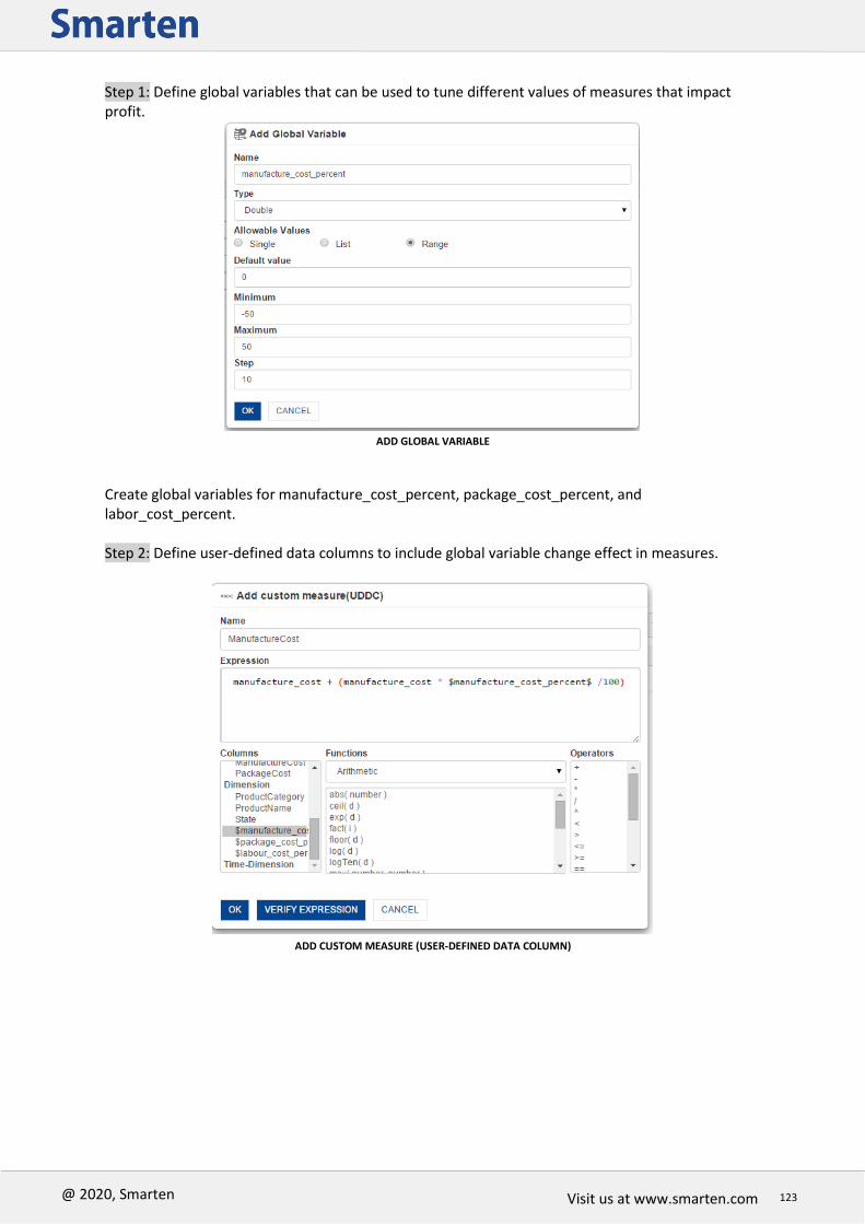
Visit us at www.smarten.com 123
@ 2020, Smarten
Visit us at
Step 1: Define global variables that can be used to tune different values of measures that impact profit.
ADD GLOBAL VARIABLE
Create global variables for manufacture_cost_percent, package_cost_percent, and labor_cost_percent. Step 2: Define user-defined data columns to include global variable change effect in measures.
ADD CUSTOM MEASURE (USER-DEFINED DATA COLUMN)

Visit us at www.smarten.com 124
@ 2020, Smarten
Visit us at
Create user-defined columns (UDDC) for ManufactureCost, PackageCost, and LaborCost using respective global variables. Expression for ManufactureCost: manufacture_cost + (manufacture_cost * $manufacture_cost_percent$ / 100) Expression for PackageCost: package_cost + (package_cost * $package_cost_percent$ / 100) Expression for LaborCost: Labor_cost + (labor_cost * $labor_cost_percent$ / 100)
Step 3: Select global variables to be included in what-if analysis.
SELECT WHAT-IF VARIABLES
The following screen shows crosstab with user-defined data columns and what-if variables. All global variables configured for What-If analysis are displayed with ranges defined for each variable.
WHAT-IF ANALYSIS
User can change any variable, and that will change all the columns that are affected by that variable. For example, changing the labor_cost_percent will affect the LabourCost, TotalCost, and Profit columns. The following screenshot shows that a 10% reduction in labor cost and a 5% reduction in manufacture cost will decrease the total cost from 8,59,35,000 to 8,04,65,250 and increase the profit from 69,70,000 to 1,24,39,750.
WHAT-IF ANALYSIS: AFTER APPLYING VARIABLE VALUE

Visit us at www.smarten.com 125
@ 2020, Smarten
Visit us at
Each time the user changes the input value of the what-if variable, it automatically recalculates the user-defined formula and shows the new result in all affected user-defined data columns. Other sample scenarios for What-If analysis:
What will be the change in the principal amount of investment if the interest rate decreases/increases by n percentage?
How will our raw material or labor costs affect the bottom line if we make percentage changes to the salary of employees?
What will be the change in profit if our product costs turn out to be 10% higher or lower than we have assumed?
What will be the change in profit if we increase production by 15%?
What will be the income tax if there is a change in the income tax slab rate by the government?
What will be the change in EMI if the interest or loan period changes?
Note:
What-If analysis is available for crosstab, graph, GeoMap, KPI, tabular, and Dashboards.
4.16 Master-Detail view in Tabular report
Master detail view in a tabular report to incorporate one to many and many to many relationships
among different dimension values. For example, if data contains purchase orders and invoices and
one purchase order has many invoices or vice versa, this view can be used to effectively show
various display and summary options to effectively reflect this master detail relationship with a
clickable view.
For example, here is the sample data with one purchase order having many invoices (one to many
relationships).
Master—Purchase Order No., Purchase Order Date, Company Name, Purchase Order Amount, Total
Invoice Amount, Pending Invoice Amount
Detail—Invoice Date, Invoice No., Item name, Invoice Amount

Visit us at www.smarten.com 126
@ 2020, Smarten
Visit us at
TABULAR REPORT: MASTER DETAIL VIEW
Note:
Master-Detail view is available for Tabular only

Visit us at www.smarten.com 127
@ 2020, Smarten
Visit us at
5 Filters and Expressions
Various kinds of filters are available in Smarten. These filters are Outliner Filters, Retrieval Filters, Dimension Filters, Measure Filters, Advanced Filters, Time Series Filters, Show/Hide Row or Column, Data Filters (Custom Cube Dimension and Custom Cube Measure Filters), and Page Filters. Filters are made interdependent throughout the system. If you have used two filters, setting value in one filter will filter values in the other filter. For example, if you have used two filters (e.g., State and City), selecting “Washington” from the state filter will display only cities in “Washington” state (e.g., Redmond and Seattle) in the city filter.
Name of the Filter Back-end Front-end
Page Filter
Retrieval Parameters
Time Series Filters
Dashboard Section Filters (All types)
Front-end Object Filters, including advanced filters (on Dimension, Measures, UDDC )
Filter is applied on cube data
Filter is applied on Front-end object data

Visit us at www.smarten.com 128
@ 2020, Smarten
Visit us at
Example of an analysis without applying any filter:
CUBE DATA
DATA ON THE FRONT-END WITHOUT APPLYING ANY FILTER
Example 1 of an analysis with the back-end and front-end filters applied:
CUBE DATA

Visit us at www.smarten.com 129
@ 2020, Smarten
Visit us at
OBJECT DATA AFTER APPLYING A BACK-END FILTER ON THE COLUMN (NO FRONT-END FILTER)
PRODUCTCATEGORY = “ALCOHOLIC DRINKS,” “COOL DRINKS,” AND “HEALTH DRINKS”
OBJECT DATA AFTER APPLYING A FRONT-END FILTER ON THE COLUMN (NO BACK-END FILTER)
PRODUCTNAME = “BEER,” “WINE,” “COLA,” AND “CHOCOLATE”
Example 2 of an analysis with the back-end and front-end filters applied:
CUBE DATA
OBJECT DATA AFTER APPLYING A BACK-END FILTER ON THE COLUMN
PRODUCTCATEGORY = “BAKERY,” “CONFECTIONARY,” AND “FRUIT JUICES”
THE DISPLAY DATA AFTER APPLYING A FRONT-END FILTER ON THE COLUMN
PRODUCTNAME = “COOKIES,” “TOFFEES,” “SODA,” “ORANGE,” AND “MANGO”
(WHILE THE BACK-END FILTER IS ALREADY APPLIED)
We can see that the product name “Soda” is included in the front-end filter condition, but it is not displayed at the front end because the ProductCategory “Cool Drinks,” which contains the product name “Soda,” is excluded by the back-end filter, and therefore the product “Soda” is not included.

Visit us at www.smarten.com 130
@ 2020, Smarten
Visit us at
5.1 Time Series (absolute, relative, range comparisons)
Time Series is defined as an ordered sequence of equally spaced time intervals. When monitoring business processes or tracking corporate business metrics, a need often arises for usage of time series data across financial and calendar years and then down to half years, quarters, months, weeks, days and dates, days of the year, and weeks of the year. Smarten built-in customizable time series lets you analyze what has changed over the previous years, half years, quarters, months, weeks, days, dates, and other critical measures.
For the dimension “Week,” Smarten uses two different types of representation for Week, i.e., Week of the Month and Week of the Year. The difference between Week of the Year and Week of the Month is as follows: In Week of the Month, each starting week of a month begins as the 1st week, whereas in Week of the Year, the starting week of January is the 1st week of the year, when the year is a calendar year, starting on 1 January.
DIFFERENT REPRESENTATIONS FOR WEEK

Visit us at www.smarten.com 131
@ 2020, Smarten
Visit us at
5.1.1 Absolute Time Series
The absolute time filtering option is used to know the value of a measure at a particular year or half year or quarter or month or week or day or date. It has no dependency or relevance to the current date. Months are displayed as M1, M2 . . . M12 for the absolute time series selection, with M1 being the first month of the year and M12 being the last month of the year. For example, if the selected date/time field has time series with start of a month as January, then M1 would be January, and M12 would be December, and if selected date/time field has time series with start month of April, then M1 would be April, and M12 would be March. Examples:
Months Year Starting from January Year Starting from April
M1 January April
M2 February May
M3 March June
M4 April July
M5 May August
M6 June September
M7 July October
M8 August November
M9 September December
M10 October January
M11 November February
M12 December March
The start month for time series on any date field can be defined through the cube definition process. Here two scenarios with different starting months are shown.
Note:
Time series hierarchy displayed in Time Series dialogue may vary based on the configuration
of time series hierarchy settings by the administrator.

Visit us at www.smarten.com 132
@ 2020, Smarten
Visit us at
5.1.2 Relative Time Series
Relative time filtering is used to know the value of a measure at a particular period relative to the current date. Here the current date value affects the definition of time series periods.
5.1.2.1 Relative Time Series filtering using full period
Filtering from start to end date for a particular period—year, half year, quarter, month, week of month, week of year or day.
RELATIVE TIME SERIES FILTER USING FULL PERIOD
Note:
All examples are based on calendar year starting from 1 Jan.
Time series hierarchy displayed in Time Series dialogue may vary based on the configuration
of time series hierarchy settings by the administrator.
Examples (without skip empty periods): Example 1: Full Data for current year and previous year
Selected Fields Result on 31 July 2013 Result on 15 July 2012
Year: Year, Year -1 Data for 2013 Data for 2012
Data for 2012 Data for 2011
Example 2: This week and previous week of current month for current year
Selected Fields Result on 31 July 2013 Result on 15 July 2013
Year: Year, Month: Month Week: Week, Week -1
Data for 5th week of July 2013 Data for 3rd week of July 2013
Data for 4th week of July 2013 Data for 2nd week of July 2013

Visit us at www.smarten.com 133
@ 2020, Smarten
Visit us at
Example 3: This week of current month of this year and previous year
Selected Fields Result on 31 July 2013 Result on 15 July 2013
Year: Year, Year -1 Month: Month Week: Week
Data for 5th week of July 2012
Data for 3rd week of July 2012
Data for 5th week of July 2013
Data for 3rd week of July 2013
Example 4: Today and yesterday of current month of this year
Selected Fields Result on 31 July 2013 Result on 15 July 2013
Day: Day, Day -1 Data for 31 July 2013 Data for 30 July 2013
Data for 15 July 2013 Data for 14 July 2013
Example 5: current half year for current year
Selected Fields Result on 31 July 2014 Result on 15 April 2014
Year: Year Half Year: Half Year
Data for July 2014
Data for Jan 2014 Data for Feb 2014 Data for Mar 2014 Data for April 2014
Example 6: current half year for current year and previous year
Selected Fields Result on 31 July 2014 Result on 15 April 2014
Year: Year, Year -1 Half Year: Half Year
Data for July 2013 Data for July 2014
Data for Jan 2013 Data for Feb 2013 Data for Mar 2013 Data for April 2013 Data for Jan 2014 Data for Feb 2014 Data for Mar 2014 Data for April 2014
Example 7: previous half year for current year
Selected Fields Result on 31 July 2014 Result on 15 June 2014
Year: Year Half Year: Half Year -1
Data from Jan 2014 to Jun 2014
Data from July 2013 to Dec 2013
Example 8: current month and previous month for current year
Selected Fields Result on 31 July 2014 Result on 15 July 2013
Year: Year, Month: Month, Month -1
Data for June 2014 Data for July 2014
Data for June 2013 Data for July 2013
Example 9: current month for current year and previous year
Selected Fields Result on 31 July 2014 Result on 15 July 2013
Year: Year, Year -1 Month: Month
Data for July 2013 Data for July 2014
Data for July 2012 Data for July 2013

Visit us at www.smarten.com 134
@ 2020, Smarten
Visit us at
Example 10: current quarter and previous quarter for current year
Selected Fields Result on 31 July 2014 Result on 15 July 2013
Year: Year Quarter: Quarter, Quarter -1
Data for April 2014 Data for May 2014 Data for June 2014 Data for July 2014
Data for April 2013 Data for May 2013 Data for June 2013 Data for July 2013
Example 11: current quarter for current year and previous year
Selected Fields Result on 31 July 2014 Result on 15 July 2013
Year: Year, Year -1 Month: Quarter
Data for July 2013 Data for July 2014
Data for July 2012 Data for July 2013
Example 12: 20th week for current year and previous year
Selected Fields Result on 31 July 2014 Result on 15 July 2013
Year: Year, Year -1 Week (Year): 20
Data for 3rd Week of May 2014 Data for 3rd Week of May 2013
Data for 3rd Week of May 2012 Data for 3rd Week of May 2013
Examples (with skip empty periods): Example 1: Full Data for current year and previous year (When data for previous year is
not present)
Selected Fields Result on 31 July 2013 Result on 15 July 2012
Year: Year, Year -1 Data for 2013 Data for 2012
Data for 2011 Data for 2010
Example 2: This month and previous month for current year (When data for previous month is not present)
Selected Fields Result on 31 July 2013 Result on 15 July 2013
Year: Year Month: Month, Month -1
Data for July 2013 Data for July 2013
Data for May 2013 Data for May 2013 Example 3: This week and previous week of current month for current year (When data for previous week is not present)
Selected Fields Result on 31 July 2013 Result on 15 July 2013
Year: Year Month: Month Week: Week, Week -1
Data for 5th week of July 2013 Data for 3rd week of July 2013
Data for 3th week of July 2013 Data for 1nd week of July 2013
Example 4: Today and yesterday (When data for yesterday is not available)
Selected Fields Result on 31 July 2013 Result on 15 July 2013
Day: Day, Day -1 Data for 31 July 2013 Data for 29 July 2013
Data for 15 July 2013 Data for 13 July 2013

Visit us at www.smarten.com 135
@ 2020, Smarten
Visit us at
Examples (without Skip to previous higher level period):
Example 1: Data for current Quarter and previous Quarter (when current Quarter is Quarter 1)
Selected Fields Result on 15 Mar 2015
Year: Year Quarter: Quarter,Quarter-1
Data for Quarter 1 of 2015
Example 2: Data for current Month and previous Month (when current Month is January)
Selected Fields Result on 31 Jan 2015
Year: Year Month: Month, Month-1
Data for Jan 2015
Example 3: Data for Week and previous Week of current Month for current Year (when
Current week is 1st Week)
Selected Fields Result on 6 Mar 2015
Year: Year Month: Month Week: Week, Week -1
Data for 1st week of Mar 2015
Examples (with Skip to previous higher level period): Example 1: Data for current Quarter and previous Quarter (when current Quarter is Quarter 1)
Selected Fields Result on 15 Mar 2015
Year: Year Quarter: Quarter,Quarter-1
Data for Quarter 1 of 2015 Data for Quarter 4 of 2014
Example 2: Data for current Month and previous Month (when current Month is January)
Selected Fields Result on 31 Jan 2015
Year: Year Month: Month, Month-1
Data for Jan 2015 Data for Dec 2014
Example 3: Data for Week and previous Week of current Month for current Year (when Current week is 1st Week)
Selected Fields Result on 6 Mar 2015
Year: Year Month: Month Week: Week, Week -1
Data for 1st week of Mar 2015 Data for 4th week of Feb 2015

Visit us at www.smarten.com 136
@ 2020, Smarten
Visit us at
5.1.2.2 Relative Time Series filtering using period to date
Filtering from the start to the current date for a particular period—for year, half year, quarter, week of month, and week of year.
RELATIVE TIME SERIES FILTER USING PERIOD TO DATE
Note:
All examples are based on calendar year starting from 1 Jan.
Time series hierarchy displayed in Time Series dialogue may vary based on the configuration
of time series hierarchy settings by the administrator.
Examples (without skip empty periods):
Example 1: Year to date data for current year and previous year
Selected Fields Result on 31 July 2014 Result on 15 July 2014
YTD: YTD, YTD -1
Data for 1 Jan to 31 July 2013 Data for 1 Jan to 31 July 2014
Data for 1 Jan to 15 July 2013 Data for 1 Jan to 15 July 2014
Example 2: Half year to date data for current half year and current year
Selected Fields Result on 31 July 2014 Result on 15 April 2014
YTD: YTD HTD: HTD
Data for 1 July 2014 to 31 July 2014
Data for 1 Jan 2014 to 15 April 2014
Example 3: Quarter to date data for previous quarter and current year
Selected Fields Result on 31 July 2014 Result on 15 July 2014
YTD: YTD QTD: QTD -1
Data for 1 Apr 2014 to 30 Apr 2014
Data for 1 Apr 2014 to 15 Apr 2014
YTD: YTD QTD: QTD -1 MTD date up to 20th
Data for 1 Apr 2014 to 20 Apr 2014
Data for 1 Apr 2014 to 20 Apr 2014

Visit us at www.smarten.com 137
@ 2020, Smarten
Visit us at
Example 4: Month to date data for current quarter and current year
Selected Fields Result on 31 July 2014 Result on 15 July 2014
YTD: YTD QTD: QTD Month: MTD MTD date up to Current Date
Data for 1 July to 31 July 2014
Data for 1 July to 15 July 2014
MTD date up to 20th Data for 1 July to 20 July 2014
Data for 1 July to 20 July 2014
Example 5: Month to date data for current year and previous year
Selected Fields Result on 31 July 2014 Result on 15 July 2014
YTD: YTD, YTD -1 QTD: QTD MTD: MTD MTD date up to Current Date
Data for 1 July to 31 July 2013 Data for 1 July to 31 July2014
Data for 1 July to 15 July 2013 Data for 1 July to 15 July 2014
MTD date up to 20 July Data for 1 July to 20 July 2013 Data for 1 July to 20 July 2014
Data for 1 July to 20 July 2013 Data for 1 July to 15 July 2014
Example 6: Month to date data for current month and previous month for current year
Selected Fields Result on 31 July 2014 Result on 15 July 2013
YTD: YTD MTD: MTD, MTD -1 MTD date up to Current Date
Data for 1 June to 30 June 2014 Data for 1 July to 31 July 2014
Data for 1 June to 15 June 2013 Data for 1 July to 15 July 2013
MTD date up to 20 July Data for 1 June to 20 June 2014 Data for 1 July to 20 July 2014
Data for 1 June to 20 June 2013 Data for 1 July to 15 July 2014
Example 7: Quarter to date data for previous quarter and current quarter of current year
Selected Fields Result on 31 March 2014 Result on 31 March 2013
YTD: YTD QTD: QTD, QTD -1
Data for 1stQtr 2014 Data for 4thQtr 2013
Data for 1stQtr 2013 Data for 4thQtr 2012

Visit us at www.smarten.com 138
@ 2020, Smarten
Visit us at
Examples (with skip empty periods):
Example 1: Year to date data for current year and previous year (When data for previous year is not present)
Selected Fields Result on 31 July 2014 Result on 15 July 2014
YTD: YTD, YTD -1 Data for 1 Jan to 31 July 2014 Data for 1 Jan to 31July 2013
Data for 1 Jan to 15 July 2014 Data for 1 Jan to 15 July 2013
Example 2: Quarter to date data for current quarter and previous quarter for current year (When data for previous quarter is not present)
Selected Fields Result on 31 July 2014 Result on 15 April 2014
YTD: YTD QTD: QTD, QTD -1
Data for 1 July 2014 to 31 July 2014 Data for 1 January 2014 to 31 January 2014
Data for 1 April 2014 to 15 April 2014 Data for 1 October 2013 to 15 October 2013
Example 3: Month to date data for current month and previous month of current year
(When data for previous month is not present)
Selected Fields Result on 31 July 2014 Result on 15 July 2014
YTD: YTD Month: MTD, MTD-1
Data for 1 July to 31 July 2014 Data for 1 May to 31 May 2014
Data for 1 July to 15 July 2014 Data for 1 May to 15 May 2014
Examples (without Skip to previous higher level period): Example 1: Quarter to date Data for current Quarter and previous Quarter (when current Quarter is Quarter 1)
Selected Fields Result on 15 Mar 2015
Year: YTD Quarter: QTD,QTD-1
Data for 1 January 2015 to 15 March 2015
Example 2: Month to date Data for current Month and previous Month (when current Month is January)
Selected Fields Result on 15 Jan 2015
Year: YTD Month: MTD, MTD-1
Data for 1 January 2015 to 15 January 2015
Example 3: Week to date Data for Week and previous Week of current Month for current Year (when Current week is 1st Week)
Selected Fields Result on 6 Mar 2015
Year: YTD Month: MTD Week: WTD, WTD -1
Data for 1st March to 6th March 2015

Visit us at www.smarten.com 139
@ 2020, Smarten
Visit us at
Examples (with Skip to previous higher level period):
Example 1: Quarter to date Data for current Quarter and previous Quarter (when current Quarter is Quarter 1)
Selected Fields Result on 15 Mar 2015
Year: YTD Quarter: QTD,QTD-1
Data for 1 January 2015 to 15 March 2015 Data for 1 October 2014 to 15 December 2014
Example 2: Month to date Data for current Month and previous Month (when current Month is January)
Selected Fields Result on 15 Jan 2015
Year: YTD Month: MTD, MTD-1
Data for 1 January 2015 to 15 January 2015 Data for 1 December 2014 to 15 December 2014
Example 3: Week to date Data for Week and previous Week of current Month for current Year (when Current week is 1st Week)
Selected Fields Result on 6 Mar 2015
Year: YTD Month: MTD Week: WTD, WTD -1
Data for 1st March 2015 to 6th March 2015 Data for 22nd February 2015 to 27th February 2015
5.1.3 Range Time Series
This option is used to filter time based on range and custom periods. Users can apply simple time filtering based on before, after, range, and other conditions.
Note:
All examples are based on calendar year starting from 1 Jan.
Time series hierarchy displayed in Time Series dialogue may vary based on the configuration
of time series hierarchy settings by the administrator.
Examples:
Options On 10 Feb 2013 On 31 July 2012 On 31 March 2011
Today 10 Feb 2013 31 July 2012 31 March 2011
This day 10th of every month 31st of every month 31st of every month
This week 2nd week of every month
5th week of every month
5th week of every month
This month 2nd month of every year
7th month of every year
3rd month of every year
This quarter 1st quarter of every year
3rd quarter of every year
1st quarter of every year
This half year 1st half year of every year
2nd half year of every year
1st half year of every year
This year 2013 2012 2011

Visit us at www.smarten.com 140
@ 2020, Smarten
Visit us at
Selected Fields Options Result on 31July 2014
Before 1 May 2014 Data up to 30 April 2014
After 10 Feb 2014 Data from 11 Feb 2014 to 31 July 2014
Between 15 March 2014 to 20 May 2014
Data from 15 March to 20 May 2014
Not Between 7 March 2014 to 1 July 2014
Data up to 6 March 2014 and Data from 2 July 2014 to 31 July 2014
5.2 Advanced Filter
The advanced filter is a type of filter that can be applied on the dimensions as well as measures. Users can create filters based on various string, arithmetic, date, statistics, trigonometry, or conditional statements using various arithmetic operators (such as +, -, /, etc.) or comparison operators (such as =, >, < etc.)
Arithmetic Functions
Functions Description
ABS Returns absolute value of a number
CEIL Returns the smallest whole number that is greater than or equal to a specified number
EXP Returns exponential value of a number
FACT Returns factorial of a number
FLOOR Returns the largest whole number that is smaller than or equal to a specified number
LOG Returns natural logarithm (base e) of a number
LOGTEN Returns decimal logarithm (base 10) of a number
MAX Returns larger of two numbers
MIN Returns smaller of two numbers
MOD Returns modulus of two numbers (the remainder after dividing the first number into the other number)
PI Returns pi (3.14159265358979323) times a number
RANDOM Returns a random whole number between two specified numbers
ROUND Returns a number rounded off decimal numbers
SIGN Returns a number (-1, 0, or 1) indicating the sign of a number
SQRT Returns the square root of a number
Statistic Functions
Functions Description
AVG Returns average value of the expression
COUNT Returns number of cases in the expression
MAXIMUM Returns maximum value of the expression
MINIMUM Returns minimum value of the expression
SUM Returns sum total of the expression

Visit us at www.smarten.com 141
@ 2020, Smarten
Visit us at
String Functions
Functions Description
ASC Returns ASCII value of a character
BOOLEANVALUE Returns contents of a string as Boolean
BYTEVALUE Returns contents of a string as byte
CHARVALUE Returns contents of an integer as character
DOUBLEVALUE Returns contents of a string as double
FILL Returns a string of a specified length filled with occurrences of a specified string
FLOATVALUE Returns contents of a string as float
INDEXOFCHAR Returns the starting position of a character within a specified string
INDEXOFSTRING Returns the starting position of a string within a specified string
INTVALUE Returns contents of a string as integer
ISDATE Determine if the specified string contains a valid date
ISNULL Determine if the argument is NULL
ISNUMBER Determine if the specified string contains a number
ISTIME Determine if the specified string contains a valid time
LEFT Returns a specified number of characters from a string, starting with the first character
LEFTTRIM Returns a copy of a specified string with leading blanks removed
LENGTH Returns length of a string
LONGVALUE Returns contents of a string as long
MATCH Returns a determination whether a string contains a particular pattern of characters
REPLACE Returns a copy of a specified string in which a specified number of characters, starting with a specified character, have been replaced with characters from another specified string
REVERSE Reverses the order or characters in a string
RIGHT Returns the specified number of characters from the end of a specified string
RIGHTTRIM Returns a copy of a specified string with trailing blanks removed
SHORTVALUE Returns contents of a string as short
SPACE Returns a string of a specified length filled with a specified number of spaces
SUBSTRING Returns a string containing a character copied (starting at a specified position and ending at a specified position) from a specified string
TOLOWERCASE Returns a copy of a specified string with all uppercase letters converted to lowercase
TOSTRING Returns a string representation of a specified object
TOUPPERCASE Returns a copy of a specified string with all lowercase letters converted to uppercase
TRIM Returns a string with leading and trailing blanks removed
TRUNCATE Returns a number truncated to a specified number of decimal places

Visit us at www.smarten.com 142
@ 2020, Smarten
Visit us at
Trigonometric Functions
Functions Description
COS Cosine of number (number in radian)
SIN Sine of number (number in radian)
TAN Tangent of number (number in radian)
Miscellaneous Functions
Functions Description
IFCASE Returns TRUE if condition is validated and returns FALSE if invalidated
WHENTHEN Tests values of a column or expression and returns values based on the results of the test
Date Functions
Functions Description
DatePart (period, source)
datePart( "d",dateTime( "2001-02-16 20:38:40")) Returns 16 datePart( "m",dateTime( "2001-02-16 20:38:40")) Returns 2 datePart( "y",dateTime( "2001-02-16 20:38:40")) Returns 2001 datePart( "q",dateTime( "2001-02-16 20:38:40")) Returns 1 datePart( "h",dateTime( "2001-02-16 20:38:40")) Returns 20 datePart( "n",dateTime( "2001-02-16 20:38:40")) Returns 38 datePart( "s",dateTime( "2001-02-16 20:38:40")) Returns 40 datePart( "w",dateTime( "2001-02-16 20:38:40")) Returns 7 Return Value: Returns an Integer value containing the specified component of a given Date value.
DateAdd (type, date, value)
dateAdd( "d",10,dateTime( "2001-02-16 20:38:40")) Returns 26-Feb-2001 20:38:40 dateAdd( "m",2,dateTime( "2001-02-16 20:38:40")) Returns 16-Apr-2001 20:38:40 dateAdd( "y",2,dateTime( "2001-02-16 20:38:40")) Returns 16-Feb-2003 20:38:40 dateAdd( "q",2,dateTime( "2001-02-16 20:38:40")) Returns 16-Aug-2001 20:38:40 dateAdd( "w",2,dateTime( "2001-02-16 20:38:40")) Returns 02-Mar-2001 20:38:40 dateAdd( "h",2,dateTime( "2001-02-16 20:38:40")) Returns 16-Feb-2001 22:38:40 dateAdd( "n",2,dateTime( "2001-02-16 20:38:40")) Returns 16-Feb-2001 20:40:40 dateAdd( "s",2,dateTime( "2001-02-16 20:38:40")) Returns 16-Feb-2001 20:38:42 Return Value: Returns a Date value containing a date and time value to which a specified time interval has been added.
DateDiff (type, date1, date2)
dateDiff("d", dateTime( "2001-02-18 20:38:40"),dateTime( "2001-02-16 20:38:40")) Returns 2 dateDiff("m", dateTime( "2001-02-16 20:38:40"),dateTime( "2001-05-16 20:38:40")) Returns -3 dateDiff("y", dateTime( "2003-02-16 20:38:40"),dateTime( "2001-02-16 20:38:40")) Returns 2 dateDiff("q", dateTime( "2001-07-16 20:38:40"),dateTime( "2001-02-16 20:38:40")) Returns 2 dateDiff("w", dateTime( "2001-02-18 20:38:40"),dateTime( "2001-02-06 20:38:40")) Returns 2 dateDiff("h", dateTime( "2001-02-16 20:38:40"),dateTime( "2001-02-16

Visit us at www.smarten.com 143
@ 2020, Smarten
Visit us at
10:38:40")) Returns 10 dateDiff("n", dateTime( "2001-02-16 20:38:40"),dateTime( "2001-02-16 20:18:40")) Returns 20 dateDiff("s", dateTime( "2001-02-16 20:38:40"),dateTime( "2001-02-16 20:38:10")) Returns 30 Return Value: Returns a Long value specifying the number of time intervals between two Date values.
MonthName (number1, [abbreviate], [number2])
monthName( 1,false, 1 ) Returns January monthName( 1,true, 1 ) Returns Jan Return Value: Returns a month name representing the month for a number from 1 to 12.
WeekdayName (number1, [abbreviate], [number2])
weekdayName( 2, true, 3) Returns Wed weekdayName( 2, false, 3) Returns Wednesday Return Value: Returns a day name representing the day of the week for a number from 1 to 7.
FormatDate (date, “string”)
FormatDate ('2001-02-16',’yy/mm/dd’) Returns 01/02/14 formatDate( dateTime( "2001-02-16 20:38:40"), "MM/dd/yyyy") Returns 02/16/2001 Return Value: Returns string of the specified format for a specified date.
date( object ) date( "2001-02-16") Returns 16-Feb-2001
dateTime( object ) dateTime( "2001-02-16 20:38:40") Returns 16-Feb-2001 20:38:40
day( date ) day( dateTime( "2001-02-16 20:38:40")) Returns 16
dayName ( date ) dayName( dateTime( "2001-02-16 20:38:40")) Returns Friday
dayNumber( date ) dayNumber( dateTime( "2001-02-16 20:38:40")) Returns 6
daysAfter( date,date ) daysAfter( dateTime( "2001-02-16 20:38:40"),dateTime( "2001-02-10 20:38:40")) Returns 6
hour( date ) hour( dateTime( "2001-02-16 20:38:40")) Returns 20
minute( date ) minute( dateTime( "2001-02-16 20:38:40")) Returns 38
month( date ) month( dateTime( "2001-02-16 20:38:40")) Returns 2
now() now() Returns 20:38:40 Return value : Returns current time
relativeDate( date, i ) relativeDate( dateTime( "2001-02-16 20:38:40"), 5 ) Returns Wed Feb 21 20:38:40 IST 2001 Return value: Returns the date that occurs n days after a given date
time( object ) time( "20:38:40") Returns 20:38:40
relativeTime( time , I ) relativeTime( time( "20:38:40"), 5 ) Returns 20:38:45 Return value: Returns the time that occurs n seconds after a given time
second( time ) second( time( "20:38:40")) Returns 40
today( ) today( ) Returns 16-Feb-2001 Return value: Returns the current system date
year( date ) year( dateTime( "2001-02-16 20:38:40")) Returns 2001

Visit us at www.smarten.com 144
@ 2020, Smarten
Visit us at
Examples:
5.3 Retrieval Parameters
Various analysis objects, such as graphs, GeoMap, crosstab, and tabular, KPIs are created from a cube, and by default, these objects are fully loaded with data from the cube. But in order to see filtered views, run time parameters – retrieval parameters are provided. Users can specify the values of the desired retrieval parameters to obtain a filtered view of crosstab, graphs, GeoMap, tabular, and KPIs. For example, the default view of Sales analysis shows the data for all States, Products, and Employees. But if you want to retrieve data only for certain States, Products, or Employees, you can select the desired values for these parameters. Hence, the Sales analysis data will be retrieved on the basis of values you selected before loading the analysis.
SETTING RETRIEVAL PARAMETER
User Mark (Executive) selects Arizona as the retrieval parameter for the Column State. Another User Joe (Senior Executive) selects Arizona, Florida, and Ohio as the retrieval parameters. Both users can get analysis data as per their selected retrieval parameters.
Note:
The retrieval parameters will be available for objects such as crosstab, graphs, GeoMap,
tabular, and KPIs and will reduce the number of records on the front-end object by filtering
cube data.
Filter Description Expression
Filter Bakery, Cool Drinks, Health Drinks category for February, April, June of current year
(ProductCategory == “Bakery” || ProductCategory == “Cool Drinks” || ProductCategory == “Bakery”) && (Month == 2 || Month == 4 || Month == 6) && (Year == 2010)
Difference of Gross Sales and Target is negative (i.e., underperforming)
(Gross Sales-Target) <= 0
Sales Quantity greater than or equal to 20,000 for the year 2010
SalesQuantity>= 20,000 && Year==2010
Filter for GrossSales greater than 10% of average GrossSales
GrossSales> (0.1 * avg(GrossSales))

Visit us at www.smarten.com 145
@ 2020, Smarten
Visit us at
5.4 Global Variables
The Global variables are defined at the cube level. They can be accessed globally with various expressions and filters for BI objects within Smarten. For example, users need to view the projection of Growth based on variable % values of Sales amount. For this, a Custom Measure Column (UDDC) Growth can be created that would be calculated on the basis of a variable X and GrossSales. This X can be created as a Global Variable and assigned different values at different times to evaluate various scenarios. Formula for Growth: GrossSales + (X*GrossSales)/100. Users can change the value of X to see different projections of Growth. Any change in X would be reflected in all analyses where the value of X is used through different expressions in filters, Custom Dimension Value (UDHC), Custom Measure Column (UDDC), and retrieval parameters. Hence it saves users from the tedious task of modifying various expressions and filter formula manually and provides simple what-if analysis scenarios. Once the global variable is defined, it would be accessible throughout the application while applying Filters, creating Custom Dimension Value (UDHC), Custom Measure Column (UDDC), and Retrieval Parameters.
Note:
Global variables are available within all BI objects (such as crosstab, graphs, GeoMap, KPIs,
dashboards, and tabular) created from a cube. Global variables created for one cube cannot
be accessed from within objects created from another cube.

Visit us at www.smarten.com 146
@ 2020, Smarten
Visit us at
CUSTOM MEASURE COLUMN (GROWTH) DERIVED USING GLOBAL VARIABLE X (VALUE: 15)
CUSTOM MEASURE COLUMN (GROWTH) DERIVED FROM MODIFIED VALUE OF GLOBAL VARIABLE X (VALUE: 20)

Visit us at www.smarten.com 147
@ 2020, Smarten
Visit us at
The value of global variable X is modified from 15 to 20. In the column Growth, new value 20 will be taken into consideration, and column values will change accordingly.
Note:
The global variables will be available for objects such as crosstab, graphs, GeoMap, tabular,
and KPIs.
5.5 Rank
Ranking is the positioning of one value in comparison with other values. It is used to display top n or bottom n data values. In Smarten, you can rank dimensions on row axis or column. The remaining values that are not part of the ranking are grouped as “others.”
5.5.1 Simple Rank
Please refer to the scenario in the following figure.
ANALYSIS WITHOUT APPLYING A RANKING
Ranking on the row summary

Visit us at www.smarten.com 148
@ 2020, Smarten
Visit us at
RANK APPLIED ON ROWS WITH SHOW OTHERS (PRODUCT CATEGORIES) FOR GROSSSALES FOR THE TOP 3
RANK APPLIED ON ROWS WITHOUT SHOW OTHERS (PRODUCT CATEGORIES) FOR GROSSSALES FOR THE TOP 3

Visit us at www.smarten.com 149
@ 2020, Smarten
Visit us at
Ranking on the column summary
RANK APPLIED ON COLUMNS (STATES) FOR GROSSSALES FOR TOP 3
Applying Rank on a particular column
User can also apply ranking on data of a particular dimension. For example, user can apply ranking on GrossSales of ProductCategory for the state of Arizona.

Visit us at www.smarten.com 150
@ 2020, Smarten
Visit us at
RANK APPLIED ON THE COLUMN FOR THE STATE OF ARIZONA
5.5.2 Band Rank
Users often need to apply ranking on the extracted data for the top n number or the bottom n number of the results. Please refer to the scenario in the following figure.
ANALYSIS WITHOUT APPLYING A RANKING
ANALYSIS WITH CONVENTIONAL RANKING FOR THE TOP 3 PRODUCT CATEGORIES IN THE STATE OF ARIZONA FOR GROSSSALES

Visit us at www.smarten.com 151
@ 2020, Smarten
Visit us at
In the above crosstab, normal ranking is applied in the ProductCategory column based on the highest GrossSales achieved by various product categories for the state of Arizona. Apparently, the gross sales figure 10197878 is equal among the product categories Bakery and Tea, but the categories are ranked at positions 1 and 2. In the case when the Band Ranking is applied to the same crosstab, results would be as below. Band Ranking:
ANALYSIS WITH BAND RANKING FOR
THE TOP 3 PRODUCT CATEGORIES IN THE STATE OF ARIZONA FOR GROSS SALES The Gross Sales figures for the categories Alcoholic Drinks and Bakery are the same, Confectionary and Cool Drinks have the same sales figure, and the categories Fruit Juices, Ice Cream, and Tea also have the same sales figure. Applying Band Ranking will give the same rank to the results with the same value as shown in the illustrated example, where Alcoholic Drinks and Bakery are on the Rank 1, Confectionary and Cool Drinks are on the Rank 2, and the categories Fruit Juices, Ice Cream, and Tea are given the Rank 3.

Visit us at www.smarten.com 152
@ 2020, Smarten
Visit us at
6 KPI
Smarten’s simplified KPIs allow the user to make clear, concise definition and tracking of various performance indicators. It helps an organization define performance at various levels and measure actual progress against targeted performance. Key Performance Indicators are quantifiable measurements of performance at various levels in an organisation. Intuitive colour highlighters ensure that users can see these indicators clearly and accurately present information to the management as well as the team members. Users can further analyse performance with easy-to-use features, such as drill down, drill through, and graphical data mining.
6.1 KPI elements & conventions
Columns Description
KPI Name Name of KPI
Period The Period based on which the KPI is calculated
Frequency “How often can we measure?” The frequency ranges from Yearly to Hourly time dimensions
Polarity If increase in value of KPI is beneficial, it is ‘High’ polarity KPI, whereas if increase is adverse, it is ‘Low’ polarity. For example, Sales is High polarity KPI, while Return Quantity is Low polarity KPI.
Previous Value Actual KPI value for previous Period
Actual Actual KPI value for the current Period
Target Target KPI value as per definition
Alert Alert threshold value as per definition. Can be manual or automatic
Warning Warning threshold value as per definition. Can be manual or automatic
Variance If the polarity is high, then Variance = Actual – Target If the polarity is low, then Variance = Target – Actual
Variance % (Variance / Target)*100
Performance % If the polarity is high, then Performance % = (Actual / Target)*100 If the polarity is low, then Performance % = (Target / Actual)*100
Performance Indicator There are three indicators in the threshold section
If the Actual value is less than the Alert value
If the Actual value is less than the Warning value and greater than the Alert value
If the Actual value is greater than the Warning value
Trend Indicator The direction of the arrow indicates the direction of the Performance Trend (up or down compared with previous period). The colour indicates performance for the current period with respect to the target. If the target is not defined, trend indicator will be shown without any colour.
Performance for the period is less than the target, and performance has declined compared with previous period.
Performance for the period is less than the target, and performance has improved compared with previous period.
Performance for the period is higher than the target, and performance has declined compared with previous period.
Performance for the period is higher than the target, and performance has improved compared with previous period.
Performance has declined compared with previous period

Visit us at www.smarten.com 153
@ 2020, Smarten
Visit us at
and Target is not defined.
Performance has improved compared with previous period and Target is not defined.
Trend chart Trend chart shows the trend line for performance over a period.
Trend indicators with example:
# KPI Performance (November 2010)
KPI Performance (December 2010)
Polarity Target Performance for the period
Performance over previous period
Display
1 1900000 1700000 High 1800000 Low Low 2 1900000 1700000 High 1600000 High Low 3 1700000 1800000 High 1900000 Low High 4 1700000 1900000 High 1800000 High High 5 1900000 1700000 High - High Low 6 1700000 1900000 High - High High
6.1.1 KPI Expressions
Refer to Analytic Functions—Functions used in Custom Measures & Custom Dimension Values Formula

Visit us at www.smarten.com 154
@ 2020, Smarten
Visit us at
7 Social BI
Smarten doubles up as a social media platform for Augmented Analytics with a dedicated feature called TeamUp. TeamUp allows users to not only share the Smarten objects with other users but also rate them and post comments for those objects. Public or private conversations—chat threads created through TeamUp allow users to converse with each other. The result is TeamUp Analytics, which enables the administrators to analyze social BI activities for important insights, such as popular data, reports or dashboards, popular conversation spots, and the overall trend and activities of users within Smarten. The following features are provided by TeamUp:
General and cube- and object-specific conversations
Average rating of each object and cube
Posting of comments, replies, and Likes for conversation threads
Referencing other objects in conversation threads
Marking object-specific conversations as favorites
Reference: Working with TeamUp

Visit us at www.smarten.com 155
@ 2020, Smarten
Visit us at
8 Access Rights & Security
8.1 Column-based Access Rights (Column Access Permission)
Dimension / Measure column-based security can be applied for all the cubes. Column Access Permission is granting or restricting access to cube dimension columns or measure columns. All the subordinate objects of a dimension, including hierarchies’ levels and members, are also secured. Column Access permissions are applied at the cube level. These are implemented by giving or limiting access to cube dimensions and measures. Example: A sales manager can view the profits made by the sales representatives. Sales representatives can only view the sales targets assigned to them. The administrator defines this Dimension / Measure column access security. Roles (users) are then linked to these column securities. By default, any role (user) has access to all dimension / measure columns in a crosstab/ tabular / graph object to which they have view access. In the example below, John is Sales Manager with access to Sales Price, Sales Qty, Target, and Profit measure columns. Smith and Richard are Sales Executives with access toSales Price, Sales Qty, and Target measure columns.
COLUMN ACCESS PERMISSION

Visit us at www.smarten.com 156
@ 2020, Smarten
Visit us at
8.2 Dimension Value–based Access Rights (Data Access Permissions)
Data value security is restricting data being retrieved by or viewed by the user. Data value security is applied at the cube level. This is implemented using an expression defined at the cube level with User/Groups permissions. Example: Regional Executives can see only the GrossSales achieved in their assigned territories. A Country Manager can see the overall GrossSales as reported by various sales representatives. The administrator defines the Dimension Value Security. Roles (users) are then linked to these dimension value securities. By default, any role (user) has access to all dimension value in crosstab / tabular / graph object to which they have view access. In the scenario below, Adams, John, and Smith are Sales Representatives, whereas David is a Country Manager.
DATA ACCESS PERMISSION

Visit us at www.smarten.com 157
@ 2020, Smarten
Visit us at
9 Delivery & Publishing Agent
Smarten’s smart delivery and publishing agent offers a flexible and intelligent information delivery mechanism, bringing corporate information into the hands of the users as and when needed in the format and via the channel they prefer.
DELIVERING AND SCHEDULING ANALYSIS OBJECTS TO USERS ANYTIME, ANYWHERE
Examples:
Schedule On Scheduler Frequency
One time on 1st January, 2015 at 1 AM
One time: 1st January, 2015 Start time: 1 hour 0 minute
Every night at 12 AM Daily Start time: 0 hour 0 minute
Every Monday morning at 5 AM Weekly: Monday Start time: 5 hour 0 minute

Visit us at www.smarten.com 158
@ 2020, Smarten
Visit us at
10 Product and Support Information
Find more information about Smarten and its features at www.smarten.com Support: [email protected] Sales: [email protected] Feedback & Suggestions: [email protected] Support & Knowledgebase Portal: support.smarten.com