
Aachendarwin.bth.rwth-aachen.de/opus3/volltexte/2014/5232/pdf/5232.pdf · Oasis,Wonderwall...
224
Aachen Department of Computer Science Technical Report Termination Analysis for Imperative Programs Operating on the Heap Marc Brockschmidt ISSN 0935–3232 · Aachener Informatik-Berichte · AIB-2013-18 RWTH Aachen · Department of Computer Science · October 2014
-
Upload
truongkhuong -
Category
Documents
-
view
232 -
download
0
Transcript of Aachendarwin.bth.rwth-aachen.de/opus3/volltexte/2014/5232/pdf/5232.pdf · Oasis,Wonderwall...

AachenDepartment of Computer Science
Technical Report
Termination Analysis for ImperativePrograms Operating on the Heap
Marc Brockschmidt
ISSN 0935–3232 · Aachener Informatik-Berichte · AIB-2013-18
RWTH Aachen · Department of Computer Science · October 2014

The publications of the Department of Computer Science of RWTH Aachen Universityare in general accessible through the World Wide Web.
http://aib.informatik.rwth-aachen.de/

Termination Analysis for ImperativePrograms Operating on the Heap
Von der Fakultät für Mathematik, Informatik undNaturwissenschaften der RWTH Aachen University zurErlangung des akademischen Grades eines Doktors der
Naturwissenschaften genehmigte Dissertation
vorgelegt von
Diplom-InformatikerMarc Manuel Johannes Brockschmidt
ausHerdecke
Berichter: Prof. Dr. Jürgen GieslProf. Dr. Samir Genaim
Tag der mündlichen Prüfung: 19. November 2013
Diese Dissertation ist auf den Internetseiten der Hochschulbibliothek online verfügbar.

Marc BrockschmidtLehr- und Forschungsgebiet Informatik [email protected]
Aachener Informatik-Bericht AIB-2013-18
Herausgeber: Fachgruppe InformatikRWTH Aachen UniversityAhornstr. 5552074 AachenGERMANY
ISSN 0935-3232

Abstract
Analysing if programs and processes terminate is one of the central topics of theoreticalcomputer science. Even though to be undecidable in general, the problem has been studiedfor decades for specific subproblems. Based on the results of this work, many small exampleprograms can be proven terminating automatically now. However, even small real-worldsystems usually cannot be handled. The focus has thus now turned towards provingtermination of programs that are in wide-spread use in common devices and computers.Two different approaches to apply termination analysis to real-world problems have
seen considerable activity in the past decade. One idea is to transform programs intoformalisms that have been studied in the past, allowing to directly use existing methodsand tools. Another trend is to leverage tools for model checking from the related field ofsafety verification to apply certain selected techniques for termination proving.
This thesis makes contributions in both of these areas. First, we discuss how to transformreal-world Java Bytecode programs into term rewriting, a simple formalism thathas been used to study termination analysis for decades. User-defined data structures aretransformed into terms, allowing to make use of the many methods originally developed forterm rewriting. Then, we present techniques to handle term rewrite systems that providepre-defined support for integers. For this, we show how using suitable transformations, apowerful termination analysis can be implemented by recursing to existing,more specialisedmethod handling either integers or terms. Finally, we present SMT-based techniques toinfer non-termination of Java Bytecode and term rewriting with integers.To improve model-checking-based approaches to termination analysis of programs re-
stricted to integers, we present a new cooperative proof framework. Its novel structureallows model checking techniques and advanced termination proving techniques from termrewriting to work together. This work can be seen as a first step towards unifying thesetwo approaches, and allows further cross-fertilisation of ideas. Based on this framework,we show how this approach can be used in alternation with non-termination techniques,further improving the precision of the overall approach.The contributions of this thesis are implemented in the fully automated termination
prover AProVE and the model checker and termination prover T2. In the annualInternational Termination Competition, AProVE has proven to be the most powerfultermination analyser for Java Bytecode programs, whereas T2 is the most powerfultermination analyser for integer programs.


Acknowledgments
First, I need to thank my PhD advisor Jürgen Giesl for giving me the opportunity towork on this exciting topic. He granted me the freedom to explore my own ideas, and wasalways available to discuss the results of these explorations. I am also very grateful toSamir Genaim for agreeing to be the second supervisor of this thesis.
For making my years as PhD student in this group as fun and entertaining as they were,I want to thank my colleagues Florian Frohn, Carsten Fuhs, Fabian Emmes, Carsten Ottoand Thomas Ströder. They always gladly served as sounding boards for ideas, distractionfrom unsolved problems and company for after-work beers. I especially want to thank mytwo Carstens (Fuhs and Otto), with whom I spent hours and hours discussing the finerdetails of the theory and practice of building termination proving tools.
Similarly, I want to thank my colleagues from the MOVES and Theory of Hybrid Systemsgroups, for many shared coffees, discussions and lunches. Many thanks have to go thecollaborators in different projects, for without them, many of my own ideas could neverhave been realised in the present form.
I also want to thank Byron Cook, and the researchers and research interns at MicrosoftResearch Cambridge for giving me an opportunity to explore new ideas, and allowingme to see research from a different perspective. My internship there was enlightening,rekindled my worn-down motivation as PhD student and helped to form my decision tostay in academia.For proof-reading preliminary versions of this thesis and providing many helpful com-
ments, I want to thank Carsten Fuhs, Carsten Otto and Florian Frohn. Without them,many ≤ would still read ≥ or leq.
Finally, I want to thank my family,my friends and especially my girlfriend, who supportedme in uncountably many ways, of which at least one is putting up with my empty gazewhile my mind is returning to some unresolved question.
Marc


Contents
1 Introduction 1
2 Termination Analysis of Java Bytecode Programs 72.1 Related Work . . . . . . . . . . . . . . . . . . . . . . . . . . . . . . . . . . 102.2 Termination Graphs . . . . . . . . . . . . . . . . . . . . . . . . . . . . . . 14
2.2.1 Symbolic States . . . . . . . . . . . . . . . . . . . . . . . . . . . . . 162.2.2 Generating Termination Graphs . . . . . . . . . . . . . . . . . . . . 25
2.3 Proving Termination via Term Rewriting . . . . . . . . . . . . . . . . . . . 362.3.1 Integer Term Rewriting . . . . . . . . . . . . . . . . . . . . . . . . . 362.3.2 Term Encoding of States . . . . . . . . . . . . . . . . . . . . . . . . 382.3.3 Transforming Termination Graphs . . . . . . . . . . . . . . . . . . . 48
2.4 Post-processing Termination Graphs . . . . . . . . . . . . . . . . . . . . . 552.4.1 Optimisations of the Term Transformation . . . . . . . . . . . . . . 552.4.2 Marking Algorithms . . . . . . . . . . . . . . . . . . . . . . . . . . 612.4.3 Annotating Distances on the Heap . . . . . . . . . . . . . . . . . . 68
2.5 Proving Non-termination of Java Programs . . . . . . . . . . . . . . . . 742.5.1 Proving States Reachable . . . . . . . . . . . . . . . . . . . . . . . 742.5.2 Finding Non-terminating States . . . . . . . . . . . . . . . . . . . . 78
2.6 Evaluation . . . . . . . . . . . . . . . . . . . . . . . . . . . . . . . . . . . . 872.7 Conclusion and Outlook . . . . . . . . . . . . . . . . . . . . . . . . . . . . 91
3 Termination Analysis of Integer Term Rewriting 933.1 Related Work . . . . . . . . . . . . . . . . . . . . . . . . . . . . . . . . . . 953.2 Proof Framework . . . . . . . . . . . . . . . . . . . . . . . . . . . . . . . . 1023.3 Simplifying Integer Term Rewrite Systems . . . . . . . . . . . . . . . . . . 1053.4 Proving Termination of Integer Rewriting . . . . . . . . . . . . . . . . . . . 1123.5 Handling Terms in Integer Term Rewriting . . . . . . . . . . . . . . . . . . 118
3.5.1 Projecting Terms onto Term Height . . . . . . . . . . . . . . . . . . 119

II Contents
3.5.2 Temporary Projections . . . . . . . . . . . . . . . . . . . . . . . . . 1273.6 Synthesising Eventual Invariants . . . . . . . . . . . . . . . . . . . . . . . . 1313.7 Proving Non-termination of Integer Term Rewriting . . . . . . . . . . . . . 134
3.7.1 Looping Non-termination . . . . . . . . . . . . . . . . . . . . . . . . 1343.7.2 Non-looping Non-termination . . . . . . . . . . . . . . . . . . . . . 136
3.8 Evaluation . . . . . . . . . . . . . . . . . . . . . . . . . . . . . . . . . . . . 1393.9 Conclusion and Outlook . . . . . . . . . . . . . . . . . . . . . . . . . . . . 142
4 Termination Analysis of Integer Transition Systems 1454.1 Integer Transition Systems . . . . . . . . . . . . . . . . . . . . . . . . . . . 1484.2 Termination Proving by Safety Proving . . . . . . . . . . . . . . . . . . . . 151
4.2.1 Iterative Construction of Termination Arguments . . . . . . . . . . 1514.2.2 Cooperative Termination Proving . . . . . . . . . . . . . . . . . . . 159
4.3 Alternating Termination/Non-termination Proving . . . . . . . . . . . . . . 1714.3.1 Synthesising Recurrent Sets . . . . . . . . . . . . . . . . . . . . . . 1714.3.2 Alternation . . . . . . . . . . . . . . . . . . . . . . . . . . . . . . . 176
4.4 Evaluation . . . . . . . . . . . . . . . . . . . . . . . . . . . . . . . . . . . . 1814.4.1 Cooperative Termination Proving . . . . . . . . . . . . . . . . . . . 1814.4.2 Alternating Termination and Non-termination Proving . . . . . . . 185
4.5 Conclusion and Outlook . . . . . . . . . . . . . . . . . . . . . . . . . . . . 186
5 Conclusion 187
Bibliography 191
Vorveröffentlichungen 209

1 Chapter 1
Introduction
There are many things that I wouldLike to say to youBut I don’t know how
Oasis, Wonderwall
Termination of programs and processes is a central topic of theoretical computer science,even though the general halting problem, i.e., the question if a given algorithm will even-tually stop on all possible inputs, was shown to be undecidable [Tur36]. Thus, no generalsolution proving termination for all program exists, but algorithms handling a subset ofprograms do exist. The last decades of research in this area have been spent on pushingthe boundaries of such partial solutions.
While intellectually challenging and thus interesting on its own, automatic terminationanalysis has many practical applications in a variety of fields. The most closely related,program verification, aims at proving that a program behaves according to a given specifica-tion. Of course, such a specification usually requires that the program eventually stops andprovides a result, or that it never stops and continues accepting (and answering) queriesfrom a user. In theorem proving, the overall validity of a proof depends on showing thatproof steps such as induction proofs use well-founded orders; a property closely relatedto termination. In computational biology, the behaviour of organisms is studied by meansof mathematical modelling and computational simulation. In this context, questions suchas “will an organism eventually reach an equilibrium?” can be handled as a problem oftermination.For a long time, due to the restrictions of available computing power, termination
was only studied for relatively simple, well-defined formalisms that are not in wide useoutside of program analysis research. Most prominent in these is term rewriting, for whichmany termination techniques were first developed and implemented in powerful tools(e.g., [Lan79, Der87, GST06, KSZM09]). These tools excel at handling user-defined datastructures such as lists or trees, but have little or no support for pre-defined domains such as

2 Chapter 1. Introduction
the integers. The results of this basic research have gradually been adapted to more widelyused formalisms. Here, the logic programming community has led the way (cf. [SD94] for anearly overview), and produced a number of powerful tools for fully automatic terminationanalysis. In a different line of research, termination analysis of imperative programminglanguages (usually C, or restricted subsets of C) have seen significant interest and tooldevelopment (e.g., early results in [CS02, BMS05a, CPR06] and many following papers).However, these approaches usually were restricted to termination arguments based oninteger variables and could not handle more complex programs that operated on user-defined data structures such as lists.One solution to extend the analysis of imperative programming languages to user-
defined data structures is a transformational approach, in which an imperative program istranslated into a term rewrite system or simple logic program, and standard tools for theseformalisms are then applied. Such approaches, leveraging the power of termination analysisfor term rewriting, have been very successful for Prolog [Sch08, SGST09, SGS+10,GSS+12] and Haskell [GRS+11]. In this thesis, we present a similar, transformationalapproach to handle Java programs. Due to the contributions of this thesis and basedon existing work for term rewriting, our tool AProVE has been the most successfultermination analyser in the annual termination competition1 for the past few years.
Structure of this thesis
All of this thesis is divided into three parts. They are bound together by the commontopic of termination proving, and ordered by (decreasing) expressiveness of the consideredinput format. Related prior work is discussed in each part, and an evaluation is providedfor each of the presented techniques independently.
In the first part (Chapter 2), we present our front-end for termination analysis of JavaBytecode programs. For this, we briefly recall termination graphs, a graph-basedformalism over-approximating all possible runs of a program.2 Then, we define int-TRSs,a simple term rewriting-based formalism with built-in integers and describe a translationof termination graphs to int-TRSs. We then present a number of post-processing steps tooptimise the term encoding of complex, possibly cyclic data structures. Finally, we discusshow to use termination graphs for non-termination proving.The second part, Chapter 3, is dedicated to termination analysis of int-TRSs. We first
discuss how to simplify the obtained int-TRSs, and then present techniques to prove theirtermination. For this, we first restrict ourselves to systems only containing integers, andthen show how to extend this to int-TRSs making use of both integers and terms.Chapter 4 is the third part, discussing termination analysis of pure integer transition
systems. They can be seen as a simplification of int-TRSs, not allowing terms to represent1For details, see http://termination-portal.org/wiki/Termination_Competition.2A complete discussion of termination graphs can be found in [Ott14].

3
data structures. We first discuss how existing techniques work, and building on this, wepresent a dramatic optimisation of these approaches using cooperation graphs. Then, wediscuss how to prove non-termination of integer programs, and how to alternate this withtermination proofs to the benefit of both proof goals.
Finally, we conclude in Chapter 5, where we discuss how the contributions of this thesiscan be used and extended to obtain a tool for real-world programs.
Contributions of this thesis
This thesis is loosely based on seven earlier, peer-reviewed papers by the author [OBvEG10,BOvEG10, BOG11, BMOG12, BSOG12, BBD+12, BCF13]. This work completes and ex-tends the previously presented techniques by adding examples, formal definitions, proofsand extensive experiments. Furthermore, this thesis presents a number of new, unpub-lished techniques for termination analysis of term rewriting with integers. In detail, thecontributions of this thesis can be summarised as follows.
Termination Analysis for Java Bytecode Programs
In a first step, we discuss a transformational termination analysis approach for JavaBytecode, building on a termination analysis for term rewrite systems with integersupport which we call int-TRSs.The basis of our work are termination graphs, an over-approximation of all program
runs of a given Java Bytecode program. We obtain such graphs by symbolicallyexecuting the input program, and all language-specific details are handled in this step.This thesis only recapitulates our previous work on obtaining such graphs. A more detaileddiscussion can be found in our papers [OBvEG10, BOvEG10, BOG11, BMOG12] and theupcoming PhD thesis of Carsten Otto [Ott14].
(i) A transformational approach to termination analysis of Java Bytecode pro-grams is presented. For this, a termination graph is constructed, and then the ob-tained termination graph is translated into an int-TRS, where user-defined datastructures are represented by corresponding terms. Due to our construction, termi-nation of the obtained int-TRS implies termination of the original program.
(ii) Handling cyclic data structures posed a problem for term rewriting-based approaches,as cycles in a data structure cannot be represented faithfully in a term encodingsuitable for efficient termination proving.
We develop a set of fully automated post-processing steps on the termination graphsin (i) to find and extract termination-relevant numerical measures of cyclic datastructures.

4 Chapter 1. Introduction
(iii) The question of non-termination, i.e., if a program or single method does not stoprunning for certain inputs, is an important part of termination analysis, and arguablymore interesting for software developers looking for problems in their software.
We present an analysis built on top of the termination graphs from (i) to prove non-termination of Java Bytecode programs. It first identifies non-terminating pro-gram states, and then verifies that these are not an artefact of the over-approximatingnature of termination graphs.
Termination Analysis of Term Rewriting with Integers
In a second step, we discuss how to extend and combine techniques for termination analysisof term rewrite systems and integer programs to handle our int-TRSs.
(iv) The int-TRSs obtained from our automatic transformation in (i) are extremely largeand crufted. On the other hand, techniques from term rewriting were historicallypredominantly used on hand-crafted examples exposing a specific type of terminationproblem.
We present a set of simplification techniques that reduce the size of the generatedint-TRSs, and remove artefacts from our transformation that are not relevant forthe termination proof.
(v) A common approach to handle user-defined data structures in termination analysisof imperative programs is to replace them by (pre-defined) measures of their size.
We show how to use a similar technique on int-TRSs, representing terms encodinguser-defined data structures by their height. To significantly strengthen the technique,we also show how to automatically extract important integer information containedin a user-defined data structure.
(vi) Existing termination analysis techniques either excel at handling programs only usingintegers, or programs only using user-defined data structures and no pre-definedoperations.
We present a new technique that allows to combine these specialised techniques whenhandling an int-TRSs, making use of one type of reasoning at a time by projectingaway incompatible parts of the problem. Then, a (partial) termination proof for thereduced problem can be lifted to the original problem.
Termination Analysis of Integer Programs
Finally, we discuss how to greatly improve existing approaches to termination analysis ofpure integer programs by combining them with techniques from termination analysis ofrewriting. The main difference to our techniques for term rewriting with integers is that

5
in such programs, we do not consider terms anymore, but in contrast to term rewriting,use a designated start location. This allows us to use existing safety provers to derivemany useful invariants supporting a termination proof, as these tools have no support forhandling terms.
(vii) Termination analyses for integer programs are often built using two separate tools.One tool is responsible for generating termination arguments based on a sequence ofsample program runs, and a second tool is used to check if the constructed terminationargument holds, or alternatively provides more program runs.
We show how to dramatically improve the performance of this approach by usingcooperation graphs that allow the two separate tools to share more information aboutthe current state of the overall proof. In this way, the right termination argument isfound earlier, and the analysis diverges less often.
(viii) Termination and non-termination proving are complimentary techniques that oftenneed to infer similar information about a program. In fact, in the process of provingone of the two, important knowledge usable by the dual proof attempt is generated.
We present an alternating termination/non-termination proving procedure, wherethe information found by a partial termination proving attempt is shared with anon-termination proving tool, and the information obtained by refuting a partialnon-termination argument can be used by the termination proving tool.
Implementation and Evaluation
The theoretical contributions developed in this thesis have been implemented in tools forautomated (non-)termination analysis, mostly in the fully automated termination proverAProVE [GTSF06] and in part in T2 [CSZ13, BCF13].
(a) Contributions (i)-(iii) have been implemented as a Java Bytecode front-endin our termination prover AProVE.
We evaluated our tool on 441 termination proving benchmarks from the annualtermination competition (cf. Sect. 2.6) and compared their performance to the com-peting tools Julia [SMP10] and COSTA [AAC+08]. Furthermore, we evaluatedeach of our contributions on its own, showing their individual usefulness.
(b) Contributions (iv)-(vi) have also been implemented in AProVE and provide theback-end to our Java Bytecode termination analysis.
Due to its nature as a back-end to other analyses, we again evaluated these techniquesusing the 441 Java Bytecode termination proving benchmarks from the annualtermination proving competition (cf. Sect. 3.8). We compared the performance of

6 Chapter 1. Introduction
our new technique to an older approach also implemented in AProVE [FGP+09].Furthermore, we individually evaluated each of the presented contributions on itsown, detailing their respective uses.
Furthermore, we compared the performance of this implementation on integer pro-grams to a number of competing tools for termination analysis of integer pro-grams [CPR06, PR07, CGB+11, FKS11, CSZ13] and our implementation of con-tribution (vii) in Sect. 4.4.
(c) Contributions (vii) and (viii) were implemented in the termination prover and modelchecker T2, developed at Microsoft Research.
Due to the still very experimental nature of the implementation of (viii), we onlyevaluated (vii) on 449 termination proving benchmarks drawn from a variety ofapplications that were also used in prior tool evaluations (e.g., from Windowsdevice drivers, the Apache web server, the PostgreSQL server, . . . ). Wecompared our implementation to the tool obtained from contributions (iv)-(vi) anda number of competing tools for termination analysis of integer programs [CPR06,PR07, CGB+11, FKS11, CSZ13].
Published vs. New Contributions
Preliminary versions of some parts of this thesis have been published by the author in 7 peer-reviewed papers [OBvEG10, BOvEG10, BOG11, BMOG12, BSOG12, BBD+12, BCF13].However, this thesis contains a number of substantial improvements over the preliminaryversions and several novel contributions:
• Contribution (i) corresponds to a subset of the papers [OBvEG10, BOvEG10].
• Contribution (ii) was partially published in [BMOG12], but in this thesis, we providea number of optimisations, definitions, and proofs missing from the paper.
• Contribution (iii) appeared as [BSOG12].
• Contribution (vii) was published as [BCF13], and this thesis extends the paper bya proof of correctness.
• Contributions (iv)-(vi) and (viii) are novel and unpublished.

2 Chapter 2
Termination Analysis of JavaBytecode Programs
Get on the rollercoasterThe fair’s in town todayY’gotta be bad enough to beat the braveSo get on the helter skelterBowl into the frayY’gotta be bad enough to beat the brave
Oasis, Fade In-Out
Termination is a central problem in program verification, both as an important propertyin software development in itself, as well as a good representative of a whole class ofprogram analysis tasks related to liveness properties of programs. However, much workon termination proving in the past has been focussed on simple, primarily theoreticalformalisms such as term rewriting. Thus, the analysis of real-world programs in an imper-ative language such as Java [GJSB05] is a significant step from such work, as it requiresto handle numerous technical details that make the programming language usable to realprogrammers, but complicate the work of verification tools:
• Due to sharing, changes via a variable x referencing the heap might be visible throughanother variable y.
• A program’s control flow may depend on the state of mutable user-defined datastructures.
• Using dynamic dispatching, the code executed by a method call may only be deter-mined at runtime, based on the types of the involved objects.
• Implicit program parts such as class initialisers greatly increase the number ofdifferent contexts in which code is executed.

8 Chapter 2. Termination Analysis of Java Bytecode Programs
• Built-in data types such as arrays, and integer and floating point numbers usuallyhave machine-dependent semantics.
To handle these problems, we use a two-step methodology. In a first step, we auto-matically generate a termination graph from the input program using symbolic execu-tion [Kin76]. In the generation of termination graphs, we already handle all language-specific details. The resulting graph is then a (relatively simple) finite representation of allpossible program evaluations and forms the basis for all subsequent analyses. By buildingon top of termination graphs, further analyses do not need to be aware of the intricaciesof the analysed programming language.
We represent user-defined data structures on the heap in our termination graphs usinga novel abstract domain. It focusses on an abstract representation of connections betweenmemory regions, while these regions themselves can be represented in detail if needed.This new domain was created with mechanisation in mind, hence it is side-stepping manyof the problematic issues encountered when implementing other heap representations.
In a second step, we build specific program analyses on top of the termination graph. Sofor example, we present a translation from termination graphs to term rewriting [BN99,TeR03] such that a termination proof for the resulting term rewrite system implies ter-mination of the original program. Based on this translation, we can then leverage thenumerous existing techniques for proving termination of term rewriting (e.g., [Der87,SD94, AG00, TeR03, HM05, GTSF06, FGM+07, FGP+09, FKS11]) to prove terminationof Java programs. We will also show related analyses that make implicit information inour termination graphs explicit as additionally introduced variables.A second analysis using termination graphs is aimed at proving non-termination of
programs. For this, we present an approach that identifies parts of the termination graphthat allow non-terminating computations. Then, heuristic methods are used to provereachability of these parts of the graph. This yields the first automated non-terminationproving technique that supports both programs using user-defined data structures on theheap and aperiodic non-terminating computations.
To generalise our approach to many more languages, and to avoid the complex syntacticaldetails of Java, we built our analysis on top of Java Bytecode [LY99] (JBC), anassembly-like object-oriented language designed as intermediate format for the executionof Java programs by a Java Virtual Machine (JVM). Moreover, JBC is alsoa common compilation target for many other object-oriented high-level languages besidesJava, such as Ruby, Python, Scala, Groovy, and Clojure.
This chapter is structured as follows. First, we give an overview of work related toour goal of (non-)termination analysis of imperative programs in Sect. 2.1. Then, weprovide a short introduction to the definition and the construction of termination graphsin Sect. 2.2. After that, we describe and prove our translation of termination graphs toterm rewriting in Sect. 2.3 to be non-termination preserving. In Sect. 2.4, we present a

9
number of post-processing steps on termination graphs that improve the precision of dataencoded into a term rewrite system, allowing to handle cyclic data structures. Anotherapplication of termination graphs is presented in Sect. 2.5, where we first discuss how toprove the reachability of certain program states using witnesses, and then describe twomethods to prove non-termination of Java programs. Finally, in Sect. 2.6, we evaluatethe implementation of all presented techniques in AProVE, also comparing it to Juliaand COSTA, the only other two tools for termination proving of JBC programs. InSect. 2.7, we conclude and discuss future directions for research.

10 Chapter 2. Termination Analysis of Java Bytecode Programs
2.1 Related Work
The basis of the presented approach to Java termination analysis has been developedin a series of papers [OBvEG10, BOvEG10, BOG11, BSOG12, BMOG12] and diplomaand bachelor theses [Bro10, vE10, Mus12]. The main difference between our approachand competing techniques is the handling of user-defined data structures. Where mostapproaches abstract data structures to integers early in the analysis process, we try to keepas much information as possible about them, and encode them as terms in the generatedterm rewrite system. Finally, our back-end can dynamically choose how to measure datastructures while constructing a termination proof.
Symbolic Execution-based Program Analyses The two-step approach to terminationanalysis based on a termination graph obtained from symbolic execution was first developedfor the analysis of Haskell [GRS+11] and Prolog [Sch08, GSS+12] programs.Similar to our approach for the analysis of Java programs, the input program is executedsymbolically to obtain a graph representing all program runs. In Haskell, this allows toeasily handle the lazy evaluation strategy, while the analysis of Prolog programs profitsfrom handling the cut in the symbolic execution phase. The graphs are then translated tovariants of term rewriting, where standard tools are applied again.
The common theme of symbolic execution to obtain graphs representing an over-approximation (or a subset of interest) of computations can also be found in super-compilation [SG95] and in termination analysis of higher-order programming [PSS97].A large class of analyses based on concolic testing (or dynamic symbolic execution) usea combination of graphs obtained from symbolic execution with concrete execution (e.g.,[GKS05, SMA05, CDE08]) to obtain a large coverage of program paths.In the abstract interpretation framework [CC77], an abstract domain is used to define
abstract states, which each represent a set of program states at a certain program location.Abstract transformers are then used to define an evaluation on such symbolic states,corresponding to the evaluation of concrete states. At certain steps, abstraction techniquesare used to let the analysis converge. Our approach is similar in spirit, but does not exactlymatch the finer details of the abstract interpretation formalism. Most importantly, ourwidening procedure (which we call merging) is context-sensitive, and the abstraction itperforms is dependent on the overall state of the symbolic execution.
Abstract Domains for Heap Representation Concise and automatable representationsof data structures on the heap, allowing to model sharing effects, have been studied forsome time. The most notable progress in this direction was made in separation logic [IO01,ORY01, Rey02], an extension to Hoare logic. It introduces a number of additional operatorsto reason about the heap, most notably ∗. This “separating conjunction” is used to denote

2.1. Related Work 11
that in ϕ∗ψ, ϕ and ψ are satisfied by disjoint (“separated”) parts of the heap. This enablesto construct compositionl proofs. To speak about pointers, separation logic uses p 7→ v
to denote that the heap maps the address p (which may also appear as integer value) tothe value v. User-defined data structures can then be defined using inductive predicates.For example, non-empty acyclic lists can be defined using list(x) = x 7→ nil ∨ (∃y.(x 7→y) ∗ list(y)). So x either points to the special nil element, signifying the empty list, or xpoints to another element y, which points to a list in a separate part of the heap.Using suitable predicates to describe data structures, separation logic formulas can be
used to develop complex and detailed proofs about heap programs. However, its inherentprecision makes the approach very hard to automate. In many cases, automatic toolsbased on separation logic are restricted to certain list structures, using built-in, hardwiredinductive predicates for them. Later work [BCC+07, YLB+08, CRB10] shows that inprinciple, the approach can be extended to also handle more general data structures, butautomatically inferring suitable predicates from input programs remains an open researchproblem.On the other hand, the path length domain [SMP10] is using a more simple heap
abstraction, in which every object is represented by the maximal path allowed in thatstructure. So a list of integers [5, 2, 9] is represented by its length 3. The analysis issupported by a number of auxiliary analyses to gain information about nullness [Spo11],sharing [SS05], reachability [NS12] and cyclicity [RS06, GZ13]. While easily automatable,the approach cannot handle termination arguments related to cyclic data structures. It isalso often too imprecise when termination depends on values nested inside of an object,i.e., in the case of nested data structures or counter variables inside of objects.
Termination Analysis of Imperative Programs Numerous methods for terminationanalysis of imperative programs have been developed in the past decade. Two large groupscan be distinguished: The first only handles integer programs and treats reading from user-defined data structures as random input, and thus cannot handle termination argumentsrelated to such structures. The second group provides methods to handle the heap, usuallyproducing an intermediate program representation based on integers and then using acorresponding back-end to prove termination.
PolyRank [BMS05a, BMS05c, BMS05d, BMS05b] performs termination analysis ofC programs restricted to integer termination arguments. Here, a front-end extracts loopsfrom the input program and transforms them into a simple integer format, and terminationarguments are then obtained by solving a constraint system for each extracted loop.
A family of tools implements a termination analysis of C programs without user-defineddata structures (or a similarly restricted language) based on a counterexample-guided ab-straction refinement (CEGAR) pattern (e.g., Terminator [CPR06], ARMC [PR07],CProver [KSTW10], TRex [HLNR10], HSF [GLPR12], and T2 [BCF13] (cf. Chap-

12 Chapter 2. Termination Analysis of Java Bytecode Programs
ter 4)). A termination proof is constructed iteratively from counter-examples, where astandard state reachability checker (e.g., [BR01, HJMS03, CKSY05, McM06, AGC12]) isemployed to check the termination argument obtained so far, and a simple rank functionsynthesis tool (e.g., [PR04a, ADFG10]) is used to improve the termination argument witheach counter-example. In this setup, the semantics and details of the handled program-ming languages are primarily handled by the used safety checker, and the rank functiontool providing the termination argument can be unaware of the details of the consideredprogramming language.
KITTeL [FKS11] implements a termination analysis for C programs based on atranslation to simple integer rewrite systems. There, values read from the heap are alwaystreated as fresh, unrestricted values. In LoopFrog [TSWK11], C programs are handledby replacing loops by summaries of their behaviour, which are obtained using a generate-and-test approach based on a library of pre-defined summary patterns.The tool Mutant [BCDO06] is an extension of Terminator, using separation
logic to represent the heap. Instead of a safety checker restricted to integer programs, ituses Sonar, which implements a symbolic execution that can track the shape and lengthof list-like data structures in a program. The termination argument construction can thenmake use of integer data and the length information provided by Sonar. The techniquerequires some limited user input to obtain inductive separation logic predicates that canbe used to symbolically represent the used (list) data structures.
Cyclist [BBC08, BGP12] implements a termination proving technique based on acyclic proof system and separation logic. While at first being restricted to data structuresprovided by the user, its successor Caber [BG13b] can infer suitable inductive predicatesfrom the input program. For the termination proof, the predicates are again annotated witha natural number (intuitively corresponding to the size of the considered data structure)and then, a variation of the size change principle [LJB01] is employed to prove termination.
Numerical abstractions of heap programs are produced by THOR [MTLT10, Mag10],which uses symbolic execution with separation logic to keep track of numerical informationabout data structures on the heap. This implicit information is made explicit in theabstraction step, which replaces heap accesses by their numerical abstractions. Similar toour translation to term rewriting, this abstraction step is non-termination preserving, soa termination proof on the resulting integer program suffices to prove termination of theoriginal program.
Finally, the tools Julia [SMP10] and COSTA [AAC+08] analyse JBC programs fortermination using abstract interpretation [CC77] with the path length domain to representthe heap. In both cases, the resulting information is used to construct a constraint logicprogram, which is then analysed by a separate prover. The focus of COSTA is an evenmore precise analysis, obtaining resource bounds for input programs, where consideredresources can be anything from used CPU cycles to memory or network accesses.

2.1. Related Work 13
Non-Termination Analysis of Imperative Programs Non-termination analysis of im-perative programs has seen far less research interest than termination analysis.
In TnT [GHM+08], non-termination of C programs is proven. For this, program runsusing loops are enumerated, where each run is in the form of a lasso (i.e., a stem followedby a cycle that may repeat). Then, a constraint solving-based method is used to identifyif there is a recurrent set of program states for this cycle, i.e., states that, when evaluatingthe cycle of the considered program run, lead back into the recurrent set. Synthesisingthese sets requires solving complex non-linear constraint systems, which tends to lead tonumerous timeouts. The tool TRex [HLNR10] uses a similar approach, but alternatesthe non-termination proof with a termination proof to let both techniques profit from eachother.For non-termination analysis of Java, we are only aware of two tools. The tool In-
vel [VR08] investigates non-termination of Java programs based on a combination oftheorem proving and invariant generation using the KeY [BHS07] system. The synthesisof non-termination arguments in Invel only has very limited support for programs operat-ing on the heap. In Julia, the constraint logic programs obtained for termination analysisare under certain circumstances precise representations of the input program [PS09]. Inthese cases, non-termination of the input program is proved if the underlying terminationchecker reports non-termination of the generated logic program.

14 Chapter 2. Termination Analysis of Java Bytecode Programs
a1 a2 a3 a4 a5 . . .
c1 c2 c5 . . .
Eval Ins Refine Eval
Eval Eval
v vv
vv
Figure 2.1: Relation between concrete evaluations and paths in the termination graph
2.2 Termination Graphs
Termination graphs play a central role in our approach to analysing Java Bytecodeprograms. In our construction, we ensure that a termination graph represents all possibleevaluations of the input program. To this end, we use symbolic evaluation starting in asymbolic start state provided together with the input program. We define the structureof our symbolic states in Sect. 2.2.1. In Sect. 2.2.1.1, we discuss how we symbolicallyrepresents sets of possible values, and present our representation of sharing effects onthe heap in detail in Sect. 2.2.1.2. A symbolic state represents a set of concrete statesthat could occur in a normal evaluation of a JBC program, and we define the exactrepresentation relation later in Sect. 2.2.1.3.
To build the termination graph, our symbolic evaluation generates a new state from aleaf in the graph whenever a deterministic evaluation is possible. When no deterministicevaluation is possible, we perform a case analysis we call state refinement, leading to severalnew successors which should allow deterministic evaluation. To mark the relationshipbetween different states, we connect them by edges corresponding to the chosen evaluationor refinement. Finally, to ensure that the resulting graph is finite, we check if our evaluationrepeatedly visits the same program position. If that is the case, we try to generalise thestates at that program position to obtain a new, more abstract state that represents allof them. The old states are then represented by that new state, i.e., they are instances ofit, and we draw instance edges to signify this. By repeating this process, we finally reacha fixed point, and all leaves in the program graph correspond to program ends, where nofurther evaluation is possible. We discuss the construction of termination graphs in detailin Sect. 2.2.2, where we will also present a number of example graphs.
By suitable restrictions on our symbolic evaluation and refinement steps, we can thusguarantee that the termination graph represents all possible program runs. This connectionis displayed in Fig. 2.1. As we can see, a sequence of concrete states c1, c2, . . . obtainedby standard JBC evaluation is usually represented by a longer sequence of states in thetermination graph, which are in turn connected by instance, refinement, and evaluationedges. So each concrete state is represented (denoted by v) by a number of symbolicstates, and these in turn form a path through the termination graph.

2.2. Termination Graphs 15
class List {List next;int val;
static boolean contains(List cur , int x) {
while (cur != null) {if (cur.val == x)
return true;cur = cur.next;
}return false;
}}
(a) Java program
00: aload_0 #load cur01: ifnull 22 #jump if null04: aload_0 #load cur05: getfield val #load cur.val08: iload_1 #load x09: if_icmpne 14 #jump if val !=x12: iconst_1 #load true13: ireturn #return true14: aload_0 #load cur15: getfield next #load cur.next18: astore_0 #store in cur19: goto 022: iconst_0 #load false23: ireturn #return false
(b) JBC for contains
Figure 2.2: Small Java example method
Limitations Our symbolic evaluation allows us to handle most features of Java Byte-code, e.g., the dynamic dispatch of methods [OBvEG10], exceptions [BOvEG10], ar-rays [BSOG12], recursion [BOG11], . . . . However, in this thesis, we only present a restrictedsubset, and only support integers1 and object instances as data. Furthermore, we do notpresent how to handle exceptions or recursive methods. As usual in program analysis, wehandle int values as the unbounded integers, but our implementation also allows to treatthem as bounded integers by suitably changing the semantics of arithmetic operations.In the following, we illustrate the basic construction of termination graphs using the
example from Fig. 2.2. On the left, in Fig. 2.2(a), the class List is displayed. The fieldsof the class allow to construct a simple linked list data structure, where the next fieldis used to point to the next list element and val allows to store an integer value. Themethod contains serves as an example for a simple, standard traversal algorithm onsuch a structure. Here, list traversal is implemented as a single loop (and not recursively),where we step to the next element in each iteration. In each step, we check if cur.valis equal to the argument x. If that is the case, we return true. Otherwise, the variablecur is advanced to the next element. Finally, if we do not return inside the loop and havereached the end of the list, we return false.
The corresponding Java Bytecode (JBC), generated by the standard javac com-piler provided by Oracle2, is displayed in Fig. 2.2(b). Java Bytecode instructionsusually work on an operand stack, which is used to store intermediate results. Programvariables are represented using local variables, comparable to a number of processor reg-
1Integers here refer to a number of primitive types in JBC, e.g., char, int and long. Furthermore,boolean values are also represented using int values, and are hence supported by the presented analysis.
2In this case, Oracle javac version 1.7.0.

16 Chapter 2. Termination Analysis of Java Bytecode Programs
isters. Instructions such as aload_0 and astore_03 are used to transfer values betweenthe operand stack and local variables. For example, aload_0 loads the value of the firstlocal variable onto the operand stack, while astore_0 stores the topmost element of theoperand stack in the first local variable. Note that JBC encodes booleans as integers andhence, the instructions 13 and 23 return integer values 0 resp. 1 instead of boolean values.
2.2.1 Symbolic States
As discussed above, our termination graphs are made up of symbolic states describing aset of “concrete” states that could be used in any standard Java Virtual Machine(JVM). In our formalism, such concrete states are also the most simple symbolic states,representing only themselves. More abstract states are obtained by replacing concretevalues in variables and object fields by symbolic values. Consequently, the shape of oursymbolic states matches that of concrete states: Each state has two parts, the call stackand the heap. In symbolic states, a third component for heap predicates is added, used todescribe the sharing of symbolic values. The call stack represents the current executionas a sequence of frames. Each frame is a triple containing its own program position, localvariable values and operand stack entries. Values of local variables and the operand stackare references, which can be resolved to actual values such as integers or objects on theheap. Local variables correspond to program variables, while the operand stack is used forintermediate results of JBC instructions.
In the following, we first discuss concrete and symbolic values in Sect. 2.2.1.1. Then, wediscuss heap predicates in detail in Sect. 2.2.1.2. Finally, in Sect. 2.2.1.3, we discuss howsymbolic states formally represent each other and concrete states, giving a connection to“real” Java Virtual Machine states.
2.2.1.1 Call Stacks, References and Abstract Values
We use an infinite set of references as values for variables and object fields. In our examples,we prefix references that can be resolved to integer values with i, and references pointingto object values with o. Finally, as names for references that are resolved to integer literals,we just use these literals and do not display their value on the heap (so in our presentation,it looks like integers can be used in place of references). Formally, integer literals like0 are a reference, and the heap maps the reference 0 to the singleton integer interval[0, 0]. Note that in a standard JVM, integers are not represented using references to theheap, but are just stored directly in local variables and the operand stack. To simplifyour representation, we also use references for integers, and have amended the semantics ofarithmetic operations to match this deviation where needed. This allows to express integer
3The prefix a indicates that an address value is manipulated, whereas the prefix i is used for integeroperations.

2.2. Termination Graphs 17
equalities implicitly, as can be seen in Fig. 2.3, where x and this.val point to the same,but unknown number.
Example 2.1 (Symbolic Java Virtual Machine State)〈00 |this :o1, x : i1, y :0 |ε〉o1:List(n = o2, v = i1)o2:List(?) i1: [1, 9]Figure 2.3: Symbolic state
A first example state is displayed in Fig. 2.3 on the right. Inits upper part, the call stack is displayed, here containingone stack frame. The three parts of the stack frame areseparated by “|”. In the example, the frame’s programcounter is at instruction 00 of some method. When not important or clear from context,we display a program position as number referring to the index of the next instructionto execute and do not show the name of the considered method.
There are three local variables, this, x, and y, containing the references o1 and i1, and0 respectively. The operand stack is empty, signified by ε. A stack of two elements r, r′
with r on top is written as r, r′ (i.e., the leftmost element is the topmost element).The lower part of the state represents the heap, resolving references to (symbolic)
values. Here, i1 points to the interval [1, 9], i.e., our symbolic state represents all thosestates where all occurrences of i1 are replaced by one value from this interval. Thereference o1 resolves to an object of type List with two fields v and n (abbreviations ofval and next). Again, the values of fields are references, namely i1 and o2. Note thati1 appears both in the variable x and in the field v. This is used to encode that we donot know the exact value here (it can be anything between 1 and 9), but only states inwhich the same value is used in both x and the field v are represented.
Finally, o2 is resolved to an unknown object of type List. We use this to denotethat in the concrete states represented by this symbolic state, the reference might beresolved to some object of type List or one of its subclasses, or that o2 is in fact thenull pointer. However, we do require that all instantiations of this value are tree-shaped.This restriction can be lifted using heap predicates.
So for our abstract domain representing states, we re-use the shape of concrete statesused in a JVM and only added symbolic values to allow to represent several cases. Forintegers, we are using a simple interval domain, but more complex domains (such as theOctagon [Min06] or Polyhedron [CH78] domains) are possible. Our domain for the heap isa novel contribution, where we use a simple abstraction for possible values (i.e., List(?)to represent a possible value) and a more involved set of heap predicates to represent theheap. We will discuss the exact form of these heap predicates in Sect. 2.2.1.2.

18 Chapter 2. Termination Analysis of Java Bytecode Programs
Example 2.2 (Symbolic Java Virtual Machine State II)〈00 |this :o2, x : i2, y :1 |ε〉〈23 |this :o1, x : i1, y :0 |ε〉o1:List(n = o2, v = i1)o2:List(n = o1, v = i3)i1: [1, 9] i2: [>0] i3:ZFigure 2.4: Symbolic state
In Fig. 2.4 on the right, we show a state with a call stackconsisting of two stack frames. The topmost stack framedetermines the next evaluation step. Calling a methodcreates a new frame on top of the stack, and the controlflow hence passes to that method. When the executionreaches a return instruction, the topmost stack frame isremoved and control passes back to the frame below, allowing to continue the evaluationafter the method call.
In the state in Fig. 2.4, we also use two new shorthands to describe integer values: i2is resolved to [> 0], which denotes the interval (0,∞), and i3 refers to Z, meaning theinterval (−∞,∞). The reference o2 is used both in the variable this of the topmost stackframe, and also as value of the field next of the object referenced by o1. Furthermore,the field next of the object to which o2 is resolved again points back to o1, so the twoList elements form a cycle.
It is important to note that without heap predicates, the abstract parts of objectsdescribed in our states are assumed to be non-sharing and tree-shaped. So in our examplestate in Fig. 2.3, the reference o2 refers to either the null pointer or an acyclic list. Thisconservative assumption about states can be weakened by heap predicates, which expressthat references also represent non-tree shapes or sharing. Of course, explicitly specifyingaliasing and sharing as in Ex. 2.2 is allowed. The reason for this default restriction isrooted in our aim of termination proving by term rewriting, which excels in representingsuch structures.
Formally, we describe states as three-tuples made up from a call stack (i.e., a non-emptysequence of stack frames),4 the heap, and a set of heap predicates, which we will discussin the next section. The heap is just a partial map from references to values. Abstractinteger values are intervals, and object instances are a pair of the object’s class and a mapfrom fields to field values. Finally, unknown objects are just a class name. For technicalreasons and in contrast to standard JBC semantics, we use a special null value on theheap, and let the heap canonically resolve the reference null to the value null.
Definition 2.3 (Symbolic States) Let Refs be a set of identifiers, ProgPos a setuniquely identifying every instruction in our program, Classnames the set of definedclasses, and FieldIDs a set describing every object field defined in our program.
4 In the case of recursion, this call stack can grow without bound, and while strategies exist to handlethis [BOG11], we will not consider them in this thesis and instead refer to [Ott14].

2.2. Termination Graphs 19
Then, our set of symbolic states is
States := SFrames+×Heap×HeapPredicates
where SFrames := ProgPos× LocVar×OpStack, LocVar := Refs∗ =:OpStack, and HeapPredicates is a set of heap predicates discussed in detail inSect. 2.2.1.2. The heap is represented as a partial map
Heap := Refs → Integers ∪ Instances ∪Classnames ∪ { null }
Finally, to represent values, we use Instances := Classnames×(FieldIDs →Refs) and integer intervals Integers := {{x ∈ Z | a ≤ x ≤ b} | a ∈ Z ∪ {−∞}, b ∈Z ∪ {∞}, a ≤ b}.
We often need to speak about references at certain points in states, i.e., “the value ofthe local variable x” or “the value of the field next of the object referred to by the localvariable x”. To formally address references like this, we use state positions. In each position,we use an “anchor” such as a local variable or an operand stack element and then lista sequence of object fields to follow. For example, if x is the first local variable of thetopmost stack frame, we describe it by lv0,0. Similarly, if we want to speak about x.next,we can use lv0,0 next. Given a state s and a position π, we use s|π to denote the referenceat position π in s.
Definition 2.4 (State Positions) Let s = (〈fr0, . . . , frn〉, h, hp) ∈ States be a statewith fri = (ppi, lvi, osi). Then SPos(s) is the smallest set containing all the sequences πwith:
• π = lvi,j where 0 ≤ i ≤ n, lvi = 〈l0, . . . , lm〉, 0 ≤ j ≤ m. Then s|π is lj.
• π = osi,j where 0 ≤ i ≤ n, osi = 〈o0, . . . , ok〉, 0 ≤ j ≤ k. Then s|π is oj.
• π = π′ v for some v ∈ FieldIDs and some π′ ∈ SPos(s) where h(s|π′) =(Cl, f) ∈ Instances and where f(v) is defined. Then s|π is f(v).
The set of references in a state s is defined as SRefs(s) := {s|π | π ∈ SPos(s)}.If we have some π = τρ ∈ SPos(s), we often write s|τ
ρ→ s|π to indicate that the sequenceρ connects s|τ to s|π on the heap.
Example 2.5 (State Positions) Let s be the state in Fig. 2.3. Then, SPos(s) ={lv0,0, lv0,1, lv0,2, lv0,0 val, lv0,0 next} and SRefs(s) = {o1, i1, 0, o2}. We have s|lv0,1 =i1 = s|lv0,0 val and as s|lv0,0 = o1 and s|lv0,0 next = o2, we also have o1
next−→ o2.

20 Chapter 2. Termination Analysis of Java Bytecode Programs
For the state s′ in Fig. 2.4, the set SPos(s′) is infinite, as the state containsa cycle on the heap. For the local variables in the two stack frames, we have{lv1,0, lv1,1, lv1,2, lv0,0, lv0,1, lv0,2} ⊆ SPos(s′), but we also have lv1,0 next . . . next ∈SPos(s′). The fact that we have a position π = lv1,0 and a field sequence τ = next nextwith s|π τ→ s|π (or s|π = s|π τ ) is even an necessary criterion for deciding that the heapof s′ contains a cycle.
Based on this, we can formally define concrete states. A concrete state correspondsto what any standard JVM would use to describe the state of an execution and hencedoes not use any symbolic values, i.e., all references only point to literal integers or objectinstances with values for all fields and we have no heap predicates:
Definition 2.6 (Concrete States) Let s = (cs, h, hp) ∈ States. We call s concreteif and only if hp = ∅ and for all r ∈ SRefs(s), we have h(r) = (Cl, f) ∈ Instances,h(r) = null, or h(r) = {c} ∈ Integers for some integer literal c ∈ Z.
Example 2.7 (Concrete Java Virtual Machine State)〈00 |this :o1, x :1, y :2 |ε〉o1:List(n = null, v = 3)
Figure 2.5: Concrete state
The state displayed in Fig. 2.5 on the right is a concretestate. The local variable this points to a one-elementList, whose only element contains the value 3. The localvariables x and y have integer values 1 and 2, respectively.
2.2.1.2 Heap Predicates
To express sharing in abstracted parts of our symbolic states (e.g., of a successor ofo2 : List(?) with some reference o3), we use heap predicates. While by default, parts of theheap that have been abstracted are restricted to tree shapes and are not allowed to share,this restriction of course needs to be weakened to be able to handle real-world Javaprograms. We do this by adding heap predicates that indicate that certain structures onthe heap may share. Our predicates are centered on the notion of connections betweenregions on the heap. Intuitively, this captures that programs only consider a small part ofthe heap at a time, but use loops or recursions to shift their focus step-by-step to anotherpart. This is mirrored in our abstract domain, where certain parts of the heap can berepresented concretely as discussed above. Connections between such detailed regions arethen represented using the heap predicates we present now.
The most simple predicate we use is r =? r′, meaning that two references with differentnames might in fact be equal. This can be used in a symbolic state to represent concrete

2.2. Termination Graphs 21
states in which two references are not equal as well as states in which they are equal. Toavoid ambiguities, we require that in r =? r′, at least one of r, r′ is resolved to an unknownobject instance (i.e., if h is the heap of the corresponding state, h(r) ∈ Classnamesor h(r′) ∈ Classnames). Without this restriction, r and r′ could be marked as equal,but point to contradictory information, e.g., r could point to a list element containing thenumber 23 and r′ to one containing the number 42.
Example 2.8 (The =? Predicate)
r r′
r1 =? r2
r r′
r1
r r′
r1 r2
Figure 2.6: Shapes allowed by “=?”
Some shapes allowed by a heap predicate r1 =?
r2 are displayed in Fig. 2.6 on the right, whereeach reference is represented by a node. Anedge between two nodes r, r′ means that thereis some field in the object instance referred to by r that contains r′. In the first shape,=? is used to express that r1 and r2 could be the same. In the second shape, this is thecase, and occurrences of r2 were replaced by r1 (hence the connection from r′ to r1). Inthe third shape, the heap predicate was just removed, expressing that the references r1
and r2 are definitely not the same. So the case depicted on the left represents both ofthe other shapes.
The predicate =? only allows to specify possible sharing at some explicitly specifiedpoint. To express that two data structures can possibly join somewhere, connected by anunknown number of fields, we use the predicate r %$ r′. We even allow the case that onereaches the other (e.g., r′ is reachable from r), but we exclude the case r = r′, and requirean extra r =? r′ for it. Formally, this means that r and r′ might have common successors,i.e., there is a reference r and sequences of fields τ, τ ′ with r τ→ r and r′ τ
′→ r (e.g., r could
be a fresh reference, or equal to r or r′). We require that one of τ, τ ′ is non-empty, i.e.,the predicate %$ does not imply a possible equality. Obviously, r %$ r′ is symmetrical.
Example 2.9 (The %$ Predicate)r1 r2 r1 r2 r1 r2
r1 r2 r1 r2
Figure 2.7: Shapes allowed by “%$”
A number of shapes allowed by a heap predicater1 %$ r2 are displayed in Fig. 2.7 on the right.Note that %$ puts only few restrictions on theshapes of represented objects. The predicatemay indicate several common successors (asin the example in the bottom right corner inFig. 2.7), or no sharing at all. We also make no restrictions on the fields used in theconsidered connections.

22 Chapter 2. Termination Analysis of Java Bytecode Programs
To handle cases where we want to express that a certain connection between tworeferences on the heap exists, we introduced the heap predicate r F99K! r′, meaning that ralways reaches r′ by a path using only the fields in the set F . So if we have a s|π F99K! s|π′in some abstract state and c is some concrete state represented by s and τ ∈ F ∗ is somesequence of fields such that π τ ∈ SPos(c), then there are two cases. Either, τ already“led past” c|π′ , i.e., there is a prefix τ− of τ such that c|π τ− = c|π′ , or τ can be extendedwith τ+ ∈ F ∗ such that c|π τ τ+ = c|π′ .
Example 2.10 (The F99K! Predicate)r1 r2n p
r1 r2n n
r1{p}99K! r2p
Figure 2.8: Shapes allowedby “99K!”
Some shapes allowed by a heap predicate r1{n, p}99K! r2 are
displayed in Fig. 2.8 on the right. Here, an edge from r
to r′ labelled with n means that r points to an objectwhose field n contains r′. Note how in the second shape,not all fields used in the parameter of the heap predicatewere used (however, if r1
n, p→ r′ in that state, then r′ alsohas to be connected to r2). The requirement on shapesrepresented by F99K! is that only fields occurring in the setof F are used, but not all have to be used. Consequently, the third shape, were a {n}99K!
predicate is used, is also represented, even though this second predicate only requires asubset of fields.
However, neither =?, %$, nor F99K! lift the restriction that abstracted data structures haveto be tree-shaped. To represent non-tree shapes, we use two additional unary predicates, ♦and F . The predicate r♦ allows acyclic non-tree data structures, e.g., the diamond shapeof the predicate symbol. More generally, r♦ allows that r has more than one connectionto one of its (possibly indirect) successors r′. So formally, there may be some reference rand two non-empty sequences of fields τ 6= τ ′ such that r τ→ r and r τ ′→ r holds.
Example 2.11 (The ♦ Predicate)r
r r′
r
r′
Figure 2.9: Shapes allowed by “♦”
Some examples for shapes allowed by the predicater♦ are displayed in Fig. 2.9 on the right. Note thatthe predicate requires no certain shape, but simplyallows to have more than one different path to asuccessor. So both having no successor at all andhaving several successor that may be reached indifferent ways is allowed. The number of different paths to a successor is not restricted,but needs to be finite (because otherwise, this indicates a cycle, which is not allowed by♦).

2.2. Termination Graphs 23
To handle cycles, we use the parametrised unary predicate F . Here, r F means thata reference c might reach or be part of a cyclic data structure. The parameter F is a setof fields used to restrict this shape, and if we wish to not use this restriction, we write (without a parameter), meaning that we want to represent every possible cyclic shapeon the heap. However, when F is used, we require that in all represented data structures,each cycle on the heap uses all the fields in F at least once. So if we have s|π F insome abstract state s, and c is a concrete state represented by s, we require that if forsome successor r of c|π we have r τ→ r, then each field of F occurs at least once in the(non-empty) field sequence τ .
Example 2.12 (The Predicate)r1 r2 r3 r4
n n n
ppp
r′1
r′2 r′3
r′4
n
n
n
n
p
p
p
p
Figure 2.10: Two doubly linked lists
Two shapes described by the heap predicater1 are displayed in Fig. 2.10 on the right,where edges are labelled with fields n and p (ab-breviations of next and prev). In the most gen-eral sense, both of the displayed lists are “cyclic”structures. However, they obviously have a dif-ferent shape, and most algorithms working onlists will show a different termination behaviouron the two lists.While for the list on the top of the figure, a standard iteration following the next field
will eventually terminate, this does not hold for the list on the bottom. The differencehere is that for the list on the top, we can find no cycle that only contains next fields, asall cycles are only constructed from both next and prev fields. On the bottom, this doesnot hold. Our parametrised heap predicate can capture this difference: While r1 {n,p}represents the list on the top of Fig. 2.10, it does not represent the list on the bottom.
2.2.1.3 State Instances
Based on these intuitive concepts, we can now consider when one state s′ is representedby another state s, denoted as s′ v s. Of course, this is only possible if s′ and s are at thesame program position of their stack frames. Furthermore, we require that for referencesin s′, their counterparts in s admit at least the same values. So if h (resp. h′) is the heap ofs (resp. s′) and π is some position in s′ referring to an integer, then we want the intervalh(s′|π) to be included in (“represented by”) the corresponding interval h(s|π) at the sameposition. For object instances, this is very similar. There, we want an instance of the sametype to exist in the more abstract state, or a completely unknown object of a sufficientlygeneral type.

24 Chapter 2. Termination Analysis of Java Bytecode Programs
When considering sharing effects, and thus heap predicates, this basic idea becomes morecomplex. Intuitively, sharing just means that there are two different “ways” to describesome object on the heap. In our case, these can be represented as positions, and sharingin s′ is then equivalent to the existence of some reference r such that there are positionsπ 6= π′ such that s′|π = r = s′|π′ . Hence, an abstraction s of s′ needs to take this intoaccount and allow this explicitly, either by reproducing s|π = s|π′ , or by allowing thissharing effect using the =? or %$ predicates. As an abstraction of s′ does not need to haveall the positions s′ has (e.g., when a list of length 10 is represented by just one unknownlist element that may have any number of successors), there are two cases to consider. Ifboth π, π′ are existing in the abstraction s, but s|π 6= s|π′ , then s|π =? s|π′ needs to beadded to allow the same sharing as in s′. If one of the positions does not exist anymore,i.e., it was abstracted away, then a predecessor that was not abstracted away needs tobe annotated using the %$ predicate. To denote this predecessor, we use the notation πs,meaning the maximal prefix τ of π such that τ ∈ SPos(s). If s is determined by context,we often drop the index. So in this last case, we require the existence of s|π %$ s|π′ .5
Similarly, already abstracted sharing effects in s′, i.e., existing heap predicates, arerequired to exist in the more abstract state s. Hence, if the positions they were referringto have been abstracted away, then heap predicates for their existing predecessors needto exists in s. So if s′|π %$ s′|π′ denotes that references at two positions are sharing, thenwe also need s|π %$ s|π′ to represent that sharing in the more abstract state.
The handling of non-tree shapes leads to similar considerations. A non-tree shape suchas a cycle exists in s′ if there is a position π with two suffixes τ 6= τ ′ such that s′|π τ = s′|π τ ′holds. For example, if τ is empty, we have a cycle (because then, s′|π = s′|π τ ′ , i.e., startingin s′|π, τ ′ “leads back” to s′|π). Such shapes have to reproduced in the more abstract states, or the corresponding heap predicates have to exist in s.While all other heap predicates extend the number of represented states, s|π F99K! s|π′
is different, as it imposes a restriction on the represented states. So here, we do not needto check if the more abstract state allows all sharing effects occurring in s′, but need tocheck if the sharing effects in s′ conform to the restriction implied by the heap predicates|π F99K! s|π′ . For this, we check if, starting in s′|π, we can find a sequence using only fieldsfrom F that leads to s′|π′ . Alternatively, we allow this connection to be abstracted awayby another heap predicate of the form r F ′99K! r′.
Definition 2.13 (State Instance) Let s′ = (〈fr′0, . . . , fr′n〉, h′, hp′) and s = (〈fr0, . . . , frn〉,h, hp) ∈ States be states with fr′i = (pp′i, lv′i, os′i) and fri = (ppi, lvi, osi). We call s′ aninstance of s (denoted s′ v s) if and only if for all 0 ≤ i ≤ n, we have ppi = pp′i and
5To make our states easier to read, we introduce a special case for references that point to non-treeshapes on the heap. If, e.g., we have c|π τ→ c|π for some non-empty sequence τ , then formally, we havec|π = c|π′ for π′ = πτ . Thus, if (some part) of this cycle is abstracted away, the representing states would need to contain s|π %$ s|π. To avoid this, we treat r and r♦ as implicit r %$ r (cf. cases(g), (h) of Def. 2.13).

2.2. Termination Graphs 25
furthermore, for all π, π′ ∈ SPos(s′):
(a) if h′(s′|π)∈ Integers and π∈SPos(s), then h′(s′|π) ⊆ h(s|π)∈ Integers.(b) if h′(s′|π) = null and π ∈ SPos(s), then h(s|π) ∈ {null} ∪ Classnames.(c) if h′(s′|π) = Cl′ ∈ Classnames and π ∈ SPos(s), then
h(s|π) = Cl ∈ Classnames and Cl′ is a (possibly non-proper) subclass of Cl.(d) if h′(s′|π) = (Cl′, e′) ∈ Instances and π ∈ SPos(s), then
h(s|π) = Cl or h(s|π) = (Cl′, e) ∈ Instances, where Cl′ must be a subclass of Cl.(e) if s′|π 6= s′|π′ and π, π′ ∈ SPos(s), then s|π 6= s|π′.(f) if s′|π =? s′|π′ and π, π′ ∈ SPos(s), then s|π =? s|π′.(g) if s′|π = s′|π′ or s′|π =? s′|π′ where h′(s′|π) 6∈ Integers ∪{null} then
π, π′ ∈ SPos(s) and s|π = s|π′ or s|π =? s|π′or {π, π′} 6⊆ SPos(s) and (s|π %$ s|π′ or π = π′ and (s|π♦ or s|π F)).
(h) if s′|π %$ s′|π′, then (s|π %$ s|π′ or π = π′ and (s|π♦ or s|π F)).(i) if there is a τ 6= ε with s′|π = s′|πτ then
π, πτ ∈ SPos(s) and s|π = s|πτor s|π F with F ⊆ τ , (i.e., F only contains fields occurring in the position τ).
(j) if there are τ 6= ε 6= τ ′ with no common prefix, s′|πτ = s′|πτ ′ and for allρ < ρ ≤ τ we have s′|πρ 6= s′|πρ and for all ρ′ < ρ′ ≤ τ ′ we have s′|πρ′ 6= s′|πρ′and h′(s′|πτ ) 6∈ Integers ∪{null}, then πτ, πτ ′ ∈ SPos(s) and s|πτ = s|πτ ′ or s|π♦.
(k) if s′|π F ′, then s|π F and F ⊆ F ′.(l) if s′|π♦, then s|π♦.
Let r F⇁ r′ hold iff there is a concrete connection r τ→ r′ for some τ using only fields in
F or r F ′99K! r′ with F ′ ⊆ F holds.Then, if there are π, π′ ∈ SPos(s) with s|π F99K! s|π′ (in the more abstract state s),
then for every sequence (in the more concrete state s′) s′|π = r0F⇁ r1
F⇁ . . . rn = s′|π′,
there is either an ri with s′|π′ = ri or ri τ→ ri+1 holds and there is a prefix τ− of τ suchthat ri τ
−→ s′|π′.
Examples of using this relation will be presented in the next section.
2.2.2 Generating Termination Graphs
Using the symbolic states we just introduced, we can now define a symbolic executionframework for Java. To illustrate the concept, we first consider a termination graphfor the contains method from Fig. 2.2 in Sect. 2.2.2.1. The result termination graph isrelatively simple and does not use heap predicates. In a second step, in Sect. 2.2.2.2, amore complex example operating on cyclic lists is presented.

26 Chapter 2. Termination Analysis of Java Bytecode Programs
〈00|c :o1, x : i1 |ε〉o1:List(?) i1:Z
A
〈01|c :o1, x : i1 |o1〉o1:List(?) i1:Z
B 〈01|c :null, x : i1 |null〉i1:Z
C
〈01|c :o2, x : i1 |o2〉o2:List(n = o3, v = i2)o3:List(?) i1:Z i2:Z
D 〈09|c :o2, x : i1 | i1,i2〉o2:List(n = o3, v = i2)o3:List(?) i1:Z i2:Z
E F:〈09|c :o2, x : i1 | i1,i1〉o2:List(n = o3, v = i1)o3:List(?) i1:Z
F
T:〈09|c :o2, x : i1 | i1,i2〉o2:List(n = o3, v = i2)o3:List(?) i1:Z i2:Z
G
〈19|c :o3, x : i1 |ε〉o3:List(?) i1:Z
H〈00|c :o3, x : i1 |ε〉o3:List(?) i1:Z
I
i1 6= i2
Figure 2.11: Termination graph for contains
2.2.2.1 A Simple Termination Graph
To generate a termination graph, we start with an abstract initial state, shown as Ain Fig. 2.11. This initial state represents all calls of contains with an acyclic list cur(abbreviated as c) and an arbitrary integer value x. From this initial state, we generate atermination graph by symbolic evaluation.
The state A is at instruction 00, i.e., the instruction aload_0 needs to be evaluated first.This is done by pushing the value of the first local variable, o1, onto the operand stack.The resulting state is displayed as B, and we added an evaluation edge from A to B toindicate how the two states are related. The next instruction, ifnull 22, performs a jumpto instruction 22 if the topmost element of the operand stack, o1, is null. In B, this is notknown yet, as o1 is resolved to List(?) on the heap, meaning that it either points to aList object or is null. Hence, we perform a case analysis, called instance refinement, thatyields two new states C and D. The two are connected to B by refinement edges, depictedusing dashed arrows. In C, o1 was resolved to be null, and consequently all occurrencesof it have been replaced by null. From C, symbolic evaluation can continue by jumpingto instruction 22 and then returning from the method. We mark this program end usingthe empty state and indicate the several execution steps to it by using a dotted edge fromC. In D, we replaced o1 by o2
6, which is resolved to a new List object on the heap, withfields containing fresh references o3 and i2. As we know nothing about the values of thesefields, we let the references point to the most general value allowed by the declared fieldtype. So o3 points to List(?), meaning any object of type List or the null pointer, andi2 is resolved to Z.
In our framework, symbolic execution is always deterministic. If a state does not allowdeterministic execution, repeated refinements are performed until it is possible. Typically,a refinement step corresponds to a simple case analysis, creating one state for each ofthe considered cases. To ensure that our termination graphs over-approximate program
6We do this regularly when adapting the value of references on the heap, to ensure a single staticassignment semantics of our termination graphs.

2.2. Termination Graphs 27
behaviour, we require that each state represented before a refinement step is representedby one of the states obtained by the refinement:
Definition 2.14 (Refinement) Let R : States → Po(States), where Po(S) den-odes the powerset of S. We call R a refinement if and only if for all s ∈ States withc ∈ States concrete and c v s, there is some s ∈ R(s) with c v s and for all s ∈ R(s),s v s holds.
To formally define specific refinements, we need some syntax that allows to manipulatestates. First, we introduce reference renamings, which allow to replace all occurrences ofa reference by another one. Additionally, we define a syntax to extend the heap to mapreferences to another value.
Definition 2.15 (Reference Renamings and Heap Extensions)Let s = (cs, h, hp) ∈ States. A (not necessarily injective) map σ : Refs → Refscan be used as a reference renaming, where sσ refers to the state in which all occurrencesof references r in local variables, on the operand stack and in instance fields have beenreplaced by σ(r). We usually write [r1/r
′1, . . . , rn/r
′n] to denote the renaming that maps ri
to r′i and behaves like the identity on every other reference.For a heap value v ∈ Integers ∪ Instances ∪Classnames ∪ { null } and a
reference r ∈ Refs, we use the notation s + {r 7→ v} to extend/modify the heap h of sby mapping r to the value v.
Example 2.16 (Simple Instance Refinement) The refinement step leading from Bto {C,D} in Fig. 2.11 can formally be described by setting D to (B + {o2 7→ List(n =o3, v = i2), o3 7→ List, i2 7→ (−∞,∞))[o1/o2] and similarly, by setting C to B[o1/null].
Our first refinement example above is very simple, as List has no subtypes and B has nosharing effects that need to be expressed using heap predicates. In general, however, moresuccessors might need to be constructed when more subclasses exist. When performing aninstance refinement on a reference pointing to a value C(?), one successor for each subclassC1 . . . Cn of C is created. Additionally, one successor state is created for the null case.
Heap predicates need to be taken into account when we choose the values of referencesfilling the newly created fields. These “inherit” heap predicates from the refined reference.So for example, if we have r1 %$ r2 and refine r1, then that means that some successorof r1 could be r2 or a successor of r2 (or symmetrically). Hence, for any fresh referencer′1 resulting from the refinement, we also need to add r′1 =? r2 to allow the case that r2
is reached in one step from r1, and r′1 %$ r2 to allow later sharing. Similarly, if we havemarked r1 as possibly being part of a cycle using r1 F , then a new successor r′1 might

28 Chapter 2. Termination Analysis of Java Bytecode Programs
either be the original reference r1, requiring the predicate r′1 =? r1, or it can share withr1 in another successor, requiring r1 %$ r′1. Of course, the new reference r′1 itself might bepart of the same cycle, requiring r′1 F . Similarly, for r1♦ with new successors r′1, r′′1 , weadd r′1 =? r′′1 , r′1 %$ r′′1 , r′1♦, and r′′1♦.
Definition 2.17 (Instance Refinement) Let s = (cs, h, hp) ∈ States with h(r) =Cl ∈ Classnames. Let Cl1, . . . , Cln be all non-abstract (not necessarily proper) sub-types of Cl. Then Rr,Cl(s) := {snull, s1, . . . , sn} is an instance refinement of s with respectto {r}.
Here, snull = s[r/null]. For each si, we choose a fresh reference ri. For all fieldsfi,1 . . . fi,mi of Cli (where fi,j has type Cli,j), a new reference ri,j is generated which pointsto the most general value vi,j of type Cli,j, i.e., (−∞,∞) for integers and Cli,j for referencetypes. Then si is (s+ {ri 7→ (Cli, fi), ri,1 7→ vi,1, . . . , ri,mi 7→ vi,mi})[r/ri], where fi(vi,j) =ri,j for all j.Moreover, new heap predicates are added in si: If s contained r′ %$ r, we add r′ =? ri,j
and r′ %$ ri,j for all j to si.7 If s contained r F99K! r′ and fi,j ∈ F , we add ri,j F99K! r′ to si.If we had r♦ in s, we add ri,j♦, ri,j =? ri,j′, and ri,j %$ ri,j′ for all j, j′ with j 6= j′ to si. Ifwe had r F in s, we add ri,j F , ri =? ri,j
8 and ri,j %$ ri,j′ for all j, j′ with j 6= j′ to si.
In our example, we can continue from state D, as deterministic evaluation is now possiblethere. The following instructions, aload_0, getfield val, and iload_1 load the valuesof cur.val (i2) and x (i1) to the operand stack, and the result is displayed as E. Thenext instruction to execute is if_icmpne, which jumps to another instruction dependingon the equality of the integer values on top of the operand stack. The values of i1 andi2, however, may be equal, or not. Our case analysis strategy from above fails in thiscase, as there is an infinite number of cases to consider. We solve this problem by justconsidering all possible outcomes of the operation and call this a state split. This results inthe states F and G, in which a leading T (resp. F) is used to indicate the truth value of theconsidered integer relation. As this case analysis is very similar to refinements, we connectthe two new states by refinement edges to E. In F, we directly used this information toadapt the state information and replaced i2 by i1, as we decided that the two values wereequal. On the other hand, G is just a plain copy of E. In F, we do not need to jump toanother program instruction, hence iconst_1 and ireturn are executed to return fromthe method, again indicated by an edge leading to the empty state.From G on, evaluation can continue after jumping to instruction 14. The following
instructions just express cur = cur.next and can be evaluated using the informationalready available in G, leading to H. However, to allow us to make use of this information
7Of course, if Cli,j and the type of r′ have no common subtype or one of them is int, then r′ =? ri,jdoes not need to be added.
8We do not need to do this if |F | > 1, as then every cycle needs to contain more than one field and thus,a field’s content may never be equal to its parent.

2.2. Termination Graphs 29
int get(int x) {List cur = this;while (x-- > 0)
cur = cur.next;return cur.val;
}
(a) get method
00: aload_0 # load this01: astore_2 # store to cur02: iload_1 # load x03: iinc 1, -1 # x = x - 106: ifle 17 # jump if i <=009: aload_2 # load cur10: getfield next # load cur.next13: astore_2 # store cur14: goto 217: aload_2 # load cur18: getfield val # load cur.val21: ireturn # return val
(b) JBC for get method
Figure 2.12: Method to get an element from list
later on, when we transform termination graphs into term rewrite systems, we label theedge with the integer relation that was checked. So in this case, the edge is labelled withi1 6= i2. In general, whenever our symbolic evaluation checks an integer relation, we use it(or its converse, if it was evaluated as false) as edge label. In later steps, when performing(non-)termination analysis, these labels are used.
From H, further evaluation just jumps back to instruction 00, leading to state I. Thatstate, however, is just a renaming of our original start state A, and consequently,A representsall cases represented by I, i.e., I v A holds. Instead of continuing our symbolic evaluation,we now use an instance edge (depicted using a double arrow) to connect I back to A, as allcomputations starting in I are also represented by the computations starting in A. Afterthis, all leaves of the termination graph are program ends, and hence, it is complete. Now,all evaluations of the method starting on non-cyclic lists are represented by our graph, i.e.,for each sequence of states obtained in a normal evaluation, we can give a correspondingsequence of termination graph nodes corresponding to it.
2.2.2.2 Termination Graphs with Heap Predicates
To illustrate how termination graphs can be generated for more complex examples, we usethe get method from Fig. 2.12. It is called on some list object with an integer parameterx and returns the x-th element. When called on a cyclic list and x is greater than the listlength, the method implements a wrap-around behaviour. The Java source code for themethod is displayed in Fig. 2.12(a), and the Java Bytecode in Fig. 2.12(b).
We start our termination graph construction with state A in Fig. 2.13. Here, the implicitvariable this is abbreviated as t, and List as L. The value of this, o1, is resolved to aList object.9 The heap predicates in A indicate that o2, the successor of o1, can be the
9This is not a restriction, as get is a non-static method and hence, a successful call to the method isonly possible on non-null objects.

30 Chapter 2. Termination Analysis of Java Bytecode Programs
same reference as o1 (corresponding to a one-element cyclic list) and that following nextpointers from o2 will eventually lead back to o1. Of course, o1 and o2 might share (thepredicate o1
{n}99K! o2 even requires it) and are thus marked with o1 %$ o2. Finally, both aremarked as being part of a cyclic structure using {n}.
Symbolic evaluation starting in A leads to state B, in which cur (abbreviated as c again)was initialised with the value of this. Further evaluation of the following instructions thenyields state C, in which x was first loaded to the operand stack, and then overwritten by thedecremented value i3 (i.e., such that the value on the operand stack remained unchanged).As with checked relations, we note arithmetic operations on the edge connecting thecorresponding states, and hence add the label i3 = i1 − 1 here. In C, we need to evaluateifle 17, which jumps to instruction 17 if the value on top of the operand stack is smallerthan or equal to 0. In our case, i1 is any integer, and hence we cannot evaluate theinstruction yet. But as before, we can perform a refinement as case analysis, resulting intwo states D and E. Here, the two cases correspond to a partition of the original integerinterval used as abstract value of the refined reference i1. More generally, we have:
Definition 2.18 (Integer Refinement) Let s = (cs, h, hp) ∈ States and let r ∈Refs with h(r) = v ⊆ Z. Let v1, . . . , vn be a partition of v (i.e., v1 ∪ . . . ∪ vn = v) withvi ∈ Integers and si = (s+{ri 7→ vi})[r/ri] for fresh references ri. Then Rr,v1,...,vn(s) :={s1, . . . , sn} is an integer refinement of s with respect to {r}.
Example 2.19 (Integer Refinement) For the integer refinement on C in Fig. 2.13,we partition the original value (−∞,∞) of C|os0,0 into {(−∞, 0], [1,∞)}. We then gen-erate the refinement successor D as (C + {i4 7→ (−∞, 0]})[i1/i4] and E as (C + {i5 7→[1,∞)})[i1/i5].
From D, evaluation leaves the loop and pushes the value of the current element onto theoperand stack. The method then returns and our analysis ends, indicated by the emptystate 2. From E, evaluation of the loop body can continue. Here, the next field of cur iswritten back to cur, and the control flow jumps back to instruction 02. The resulting stateF is at the same program position as state B. Other than in our simple continue examplefrom above, neither F v B nor B v F holds. To ensure that our termination graphs arefinite, we merge states whenever we reach a program position a second time in one pathof our symbolic evaluation. Merging is a targeted widening of the constraints encoded inour states, leading to a fresh state that represents all concrete states represented by theoriginal states. We can continue our analysis from this new state. Repeated merging at thesame program position leads to more abstract states, until the analysis finally converges.For this, we use an increasingly aggressive merging strategy. Whereas at the beginning,

2.2. Termination Graphs 31
〈00|t :o1, x : i1 |ε〉o1:L(n=o2,v= i2) i2:Zo2:L(?) o1, o2{n} i1:Zo2=?o1 o2%$o1 o2
{n}99K! o1
A
〈02|t :o1, x : i1, c :o1 |ε〉o1:L(n=o2,v= i2) i2:Zo2:L(?) o1, o2{n} i1:Zo2=?o1 o2%$o1 o2
{n}99K! o1
B
〈06|t :o1, x : i3, c :o1 | i1〉o1:L(n=o2,v= i2) i2:Zo2:L(?) o1, o2{n} i1:Zi3:Zo2=?o1 o2%$o1 o2
{n}99K! o1
C〈06|t :o1, x : i3, c :o1 | i4〉o1:L(n=o2,v= i2) i2:Zo2:L(?) o1,o2{n} i4: [≤0]i3:Zo2=?o1 o2%$o1 o2
{n}99K! o1
D
〈06|t :o1, x : i3, c :o1 | i5〉o1:L(n = o2,v= i2) i2:Zo2:L(?) o1,o2{n} i5: [>0]i3:Zo2=?o1 o2%$o1 o2
{n}99K! o1
E〈02|t :o1, x : i3, c :o2 |ε〉o1:L(n = o2,v= i2) i2:Zo2:L(?) o1,o2{n} i3:Zo2=?o1 o2%$o1 o2
{n}99K! o1
F
〈02|t :o1, x : i3, c :o3 |ε〉o1:L(n = o2,v= i2) i2:Zo2:L(?) o3:L(?) i3:Zo1=?o2 o1=?o3 o2=?o3o1%$o2 o1%$o3 o2%$o3o2{n}99K! o3 o3
{n}99K! o1o1,o2,o3{n}
G
〈06|t :o1, x : i6, c :o3 | i3〉o1:L(n = o2,v= i2) i2:Zo2:L(?) o3:L(?) i3:Zo1=?o2 o1=?o3 o2=?o3o1%$o2 o1%$o3 o2%$o3o2{n}99K! o3 o3
{n}99K! o1o1,o2,o3{n} i6:Z
H
〈06|t :o1, x : i6, c :o3 | i7〉o1:L(n = o2,v= i2) i2:Zo2:L(?) o3:L(?) i7: [≤0]o1=?o2 o1=?o3 o2=?o3o1%$o2 o1%$o3 o2%$o3o2{n}99K! o3 o3
{n}99K! o1o1,o2,o3{n} i6:Z
I
〈06|t :o1, x : i6, c :o3 | i8〉o1:L(n = o2,v= i2) i2:Zo2:L(?) o3:L(?) i8: [>0]o1=?o2 o1=?o3 o2=?o3o1%$o2 o1%$o3 o2%$o3o2{n}99K! o3 o3
{n}99K! o1o1,o2,o3{n} i6:Z
J
〈10|t :o1, x : i6, c :o3 |o3〉o1:L(n = o2,v= i2) i2:Zo2:L(?) o3:L(?)o1=?o2 o1=?o3 o2=?o3o1%$o2 o1%$o3 o2%$o3o2{n}99K! o3 o3
{n}99K! o1o1,o2,o3{n} i6:Z
K
〈10|t :o1, x : i6, c :o3 |o3〉o1:L(n = o2,v= i2) i2:Zo2:L(?) o3:L(?)o1=?o2 o2=?o3o1%$o2 o1%$o3 o2%$o3o2{n}99K! o3 o3
{n}99K! o1o1,o2,o3{n} i6:Z
L
〈02|t :o1, x : i6, c :o2 |ε〉o1:L(n = o2,v= i2) i2:Zo2:L(?) o1,o2{n} i6:Zo1=?o2 o1%$o2 o2
{n}99K! o1
P
〈10|t :o1, x : i6, c :o1 |o1〉o1:L(n = o2,v= i2) i2:Zo2:L(?) o1,o2{n} i6:Zo1=?o2 o1%$o2 o2
{n}99K! o1
M
〈10|t :o1, x : i6, c :o4 |o4〉o1:L(n = o2,v= i2) i2:Zo4:L(n = o5,v= i9) i9:Zo2:L(?) o5:L(?)o1=?o2 o2=?o4o1=?o5 o2=?o5 o4=?o5o1%$o2 o1%$o4 o2%$o4o1%$o5 o2%$o5 o4%$o5o2{n}99K! o4 o5
{n}99K! o1o1,o2,o4,o5{n} i6:Z
N〈02|t :o1, x : i6, c :o5 |ε〉o1:L(n = o2,v= i2) i2:Zo2:L(?) o5:L(?)o1=?o2 o1=?o5 o2=?o5o1%$o2 o1%$o5 o2%$o5o2{n}99K! o5 o5
{n}99K! o1o1,o2,o5{n} i6:Z
O
i3= i1−1
i4 ≤ 0i5>
0
i6=i3 −
1
i7 ≤ 0
i8>
0
Figure 2.13: Termination graph for get

32 Chapter 2. Termination Analysis of Java Bytecode Programs
the merging process is aimed towards producing the most concrete state that representsboth merged states, we abstract more aggressively later on, e.g., by not choosing the unionof integer intervals as abstract value, but enlarging the value to Z.
To find such a merged state, we compare the values at all positions in the two consideredstates and from this, generate suitably general values. As example, consider the positionπ = lv0,2, i.e., the third local variable, cur. In B, this contains o1, the first element of ourlist, which is resolved to List(next = o2, val = i2) on the heap. In F, the same positioncontains o2, as we iterated to the next element. Now, o2 is resolved to List(?) in F. Thisis more abstract, and hence the merged state G has a fresh reference o3 at this position,being resolved to List(?) as well. Similarly, we have to introduce new heap predicates tofaithfully represent all sharing effects. For example, for π′ = lv0,0, i.e., the local variablethis, we have B|π = o1 = B|π′ , but F|π = o1 6= o2 = F|π′ . To represent both cases, wehave added G|π =? G|π′ to G. In the same manner, the remaining heap predicates canbe generated. The merging procedure follows the structure of Def. 2.13, and details aredocumented in [Ott14].
In G, we have references for three list elements, namely o1 representing the “first” element,o2, its successor, and o3, the value of cur. Our equality heap predicates allow all of thesereferences to be the same, corresponding to the case of the one-element list. Furthermore,we use {n}99K! to mark that o2 is connected to o3 via a sequence of n fields, just as o3 mustagain lead back to o1, as we are considering a cyclic list. Of course, these three referencesmay also share, and thus we introduce %$ predicates. As they are also part of a cyclic datastructure, we add suitable predicates, too. We now draw instance edges from B and Fto our new state G, indicating that it represents a superset of the two original states.
From G, we can restart our symbolic evaluation, which is again similar to the evaluationstarting from B. We reach instruction 06 in state H, in which we need to perform aninteger refinement to be able to decide if we continue in the loop. Between G and H, wereplaced i5 in x by a reference to i6, obtained by decrementing the old value i5 of x. Theinteger refinement in H yields two successors I and J, where I like D before leads to aprogram end. From J, our evaluation continues to state K at instruction 10. Here, o3, thevalue of cur, was loaded to the operand stack, and now the instruction getfield nextis to be executed. However, the heap of K resolves o3 to an unknown object instance oftype List. To access the next field, we need to perform an instance refinement as inDef. 2.17. In K, this is not yet possible: Remember that we require that no two referencespointing to concrete object instances may be connected with =?, but this is the case foro1 and o3. So first, we have to resolve this possible equality. To this end, we again performa case analysis, generating two successors M and L. M corresponds to the case that thecurrent value of cur (o3), is the same as this (o1), and consequently, the refined statelooks like the state B. Consequently, the computation starting in M looks just like the firstconsidered loop iteration in B-F. In L, on the other hand, we assume the two references

2.2. Termination Graphs 33
to be unequal, marking this by just removing the predicate o1 =? o3.
Definition 2.20 (Equality Refinement) Let s = (cs, h, hp) ∈ States and r =? r′ ∈hp. Hence, one of h(r) ∈ Classnames or h(r′) ∈ Classnames holds. Withoutloss of generality, let h(r) ∈ Classnames. Then Rr,r′(s) := {s=, s6=} is an equalityrefinement of s with regard to {r, r′} with s= := s[r/r′] and s 6= := (cs, h, hp \ {r =? r′}).
Example 2.21 (Equality Refinement) For the field access of K in Fig. 2.13, we wantto perform an instance refinement on K|os0,0 , but have K|os0,0 =? K|lv0,0 . We resolve thisby an equality refinement with new successors L and M, where M = K= = K[o3/o1]. Weobtain L by removing K|os0,0 =? K|lv0,0 from K.
In L, we can now perform the instance refinement. Here, we can make use of the heappredicate o3
{n}99K! o1. This requires that every represented state connects o3 again to o1, butthis would not be the case if o3 were null (as null is obviously not connected to anything).Consequently, in our instance refinement, we need only one successor state, N.10 In N, o3
has been replaced by o4, which points to a new object instance List(next = o5, val = i9).New values for o5 and i9 have been introduced, and o5 inherits a plethora of heap predicatesfrom its predecessor o4. It may be equal to any of the other list elements we keep in thestate, shares with all of them, and is also marked as cyclic. Furthermore, we know thato5 has to finally reach o1 again using n fields, and we have removed the correspondingpredicate for o4, as it already has a n successor. From N, evaluation can continue, replacingo4 as content of cur by o5. As then, o4 is not used in any local variable, operand stackentry, or object field, we remove all information about it from the state, obtaining O. Thisnew state is just a renaming of G, so we can again draw an instance edge, finishing theconstruction of the termination graph for get.We now define termination graphs formally. For this, we use the set RelOp = {i ◦ i′ |
i, i′ ∈ Refs, ◦ ∈ {<,≤,=, 6=,≥, >}} of integer relations such as i7 < 011 and the set ofarithmetic operations ArithOp = {i = i′ ./ i′′ | i, i′, i′′ ∈ Refs, ./ ∈ {+,−, ∗, /,%}} todenote the set of arithmetic computations such as i6 = i5 − 1.Termination graphs are constructed by repeatedly expanding those leaves that do not
correspond to program ends. Whenever possible, we use symbolic evaluation on a states to generate a new state s′, denoted s SyEv−→ s′. Here, SyEv−→ extends the usual evaluationrelation for JBC such that it can also be applied to symbolic states, as presented above.For a formal presentation of this, we refer to [Ott14]. In the termination graph, the corre-sponding evaluation edges are labelled by a set C ⊆ ArithOp∪RelOp which corresponds10Formally, we produce a successor for the null case and then ignore it in the symbolic execution, as it
is inconsistent and hence represents no concrete states.11Remember, we use integer constants c ∈ Z as references which always resolve to [c, c] ∈ Integers.

34 Chapter 2. Termination Analysis of Java Bytecode Programs
to the arithmetic operations and (implicitly) checked relations in the evaluation. As ex-ample, consider state I from Fig. 2.13, from which ifle 17 was evaluated by jumping toinstruction 17. There, the edge from I to its successor is labelled with i7 ≥ 0 to reflect theperformed check. Similarly, when performing arithmetic, as between states G and H, weadd corresponding labels.If symbolic evaluation is not possible, we (repeatedly) refine the information for some
references by case analysis and connect the resulting states by refinement edges. To obtaina finite graph, we create a more general state by merging whenever a program position isvisited a second time in our symbolic evaluation and add appropriate instance edges tothe graph. However, we require all cycles of the termination graph to contain at least oneevaluation edge. By using an appropriate strategy for merging states, we can automaticallygenerate a finite termination graph for any program.
Definition 2.22 (Termination Graph) A graph (V,E) with V ⊆ States, E ⊆ V ×({EvalC | C ⊆ (ArithOp ∪ RelOp)} ∪ {RefineR | R ⊆ Refs} ∪ {Ins}
)× V is a
termination graph if every cycle contains at least one edge labelled with some EvalC andone of the following holds for each s ∈ V :
• s has just one outgoing edge (s,EvalC , s′), sSyEv−→ s′, and C is the set of integer
relations that are checked (resp. generated) in this step.
• the outgoing edges of s are (s,RefineR, s1), . . . , (s,RefineR, sn) and {s1, . . . , sn}is a refinement of s according to Def. 2.18, 2.20, or 2.17 with respect to the referencesR.
• s has just one outgoing edge (s, Ins, s′) and s v s′.
• s has no outgoing edge and s = (ε, h, hp) (i.e., s is a program end).
The following soundness theorem connects the semantics of standard Java programsto the semantics of our termination graphs. It states that any evaluation on concretestates, representing states of a standard Java Virtual Machine, is representedby a sequence of abstractions, refinements, and an evaluation step in the correspondingtermination graph. The intuition for this theorem is given in Fig. 2.1.

2.2. Termination Graphs 35
Theorem 2.23 (Symbolic Evaluation Simulates Evaluation of Concrete States)Let c, c′, s ∈ States, where c is concrete, c′ is obtained by standard evaluationfrom c, c v s, and s occurs in a termination graph G. Then G contains a paths(
Ins−→ ∪ RefineR−→)∗◦ EvalC−→ s′ such that c′ v s′.
The proof of Thm. 2.23 is rather involved and is not reproduced here. Instead, werefer to [Ott14] for a full proof also handling programs using recursion and arrays, or to[BOvEG10] for a proof of this theorem for relatively simple states comparable to the onesused here. Based on Thm. 2.23, we can now define properties of termination graphs, liftingthem from single computations. Our main goal, termination proving, is supported by thefollowing definition:
Definition 2.24 (Well-founded Termination Graphs) Let G = (V,E) be a termi-nation graph. We call G well-founded if all executions starting in a concrete state c ∈States with c v s ∈ V are finite.
In the next section, we discuss how to prove a termination graph well-founded by provingtermination of a term rewrite system obtained from the graph.

36 Chapter 2. Termination Analysis of Java Bytecode Programs
2.3 Proving Termination via Term Rewriting
Termination graphs provide a concise representation of all possible program runs. As allJBC-specific features have been handled by symbolic execution during the constructionof the graph, further analyses are considerably simplified, as they only need to take thefar simpler semantics of the graph into account. Based on this, we now present a non-termination preserving translation from termination graphs to term rewriting. A standardtermination prover for term rewriting with support for built-in integers can be used onthe resulting term rewrite system, and if it succeeds, we can also conclude terminationof the original Java Bytecode program. First, we introduce int-term rewrite sys-tems, a special form of term rewrite systems, providing built-in support for integers inSect. 2.3.1. Then, we describe how to transform single references and then states into termsin Sect. 2.3.2. Building on this, we discuss how to translate entire termination graphsinto a term rewrite system in Sect. 2.3.3 and finally, in Sect. 2.4.1, we show a number ofoptimisations of this process.
2.3.1 Integer Term Rewriting
For an introduction to standard term rewriting, we refer to [BN99] and [TeR03]. We repre-sent an extension of rewriting that includes support for pre-defined operations on integernumbers. First, we fix the structure and semantics of the considered integer expressions.
Definition 2.25 (int-terms and int-constraints) Let Σpre = Z∪{+,−, ∗, /,%} be thesignature of the integers and their pre-defined operations. An int-term t ∈ T (Σpre,V) is aterm containing only symbols from Σpre and variables from V, and an atomic int-constraints ◦ t is constructed from int-terms s, t, and ◦ ∈ {<,≤,=, 6=,≥, >}. We usually use infixnotation (e.g., we write “x < y + 1” instead of “< (x,+(y, 1))”). An int-constraint is aconjunction of atomic int-constraints.
Like in standard rewriting, we additionally allow to represent user-defined data structuresby using a signature Σc for data constructors and represent program positions (or functions)by a separate signature Σd for defined symbols, such that Σpre,Σc,Σd are pairwise disjoint.Intuitively, we let a term correspond to a program state, where its root symbol defines thecurrent program position and the arguments correspond to the values of local variablesand the operand stack.
Definition 2.26 (Terms, Positions, Substitutions) Let V be a set of variables andΣ be some signature, where each symbol f ∈ Σ has a fixed arity ar(f) ∈ N0 determining thenumber of its arguments. Then, the set of terms T (Σ,V) is the smallest set that containsV and f(t1, . . . , tn) for every f ∈ Σ, where n = ar(f) and t1, . . . , tn ∈ T (Σ,V).

2.3. Proving Termination via Term Rewriting 37
We can address certain subterms of a term t = f(t1, . . . , tn) using positions. The setPos(t) of positions of t is defined as ε ∪ {i p | 1 ≤ i ≤ n and p ∈ Pos(ti)}. We use t|p todenote the subterm of t at position p, where t|ε := t and t|i p := ti|p.
We use substitutions σ ∈ V → T (Σ,V) to instantiate variables with more concretevalues. We extend this to terms by defining
σ(t) :=
σ(v) if t = v ∈ V
f(σ(t1), . . . , σ(tn)) if t = f(t1, . . . , tn)
We usually write [v1/t1, . . . , vn/tn] to denote the substitution that instantiates each vi byti. We call σ applicable to an int-constraint ϕ if σ(x) ∈ Z for all x ∈ V(ϕ), and ϕσ isvalid if it holds w.r.t. usual integer arithmetic and theory.
Example 2.27 (User-defined Data Structures as Terms) We model lists using abinary constructor symbol List and a constant Nil. For example, the list [1, 4, 3, 4] can berepresented as List(List(List(List(Nil, 4), 3), 4), 1).
The rewrite relation of an int-TRS is defined as in standard term rewriting, but weallow every rule to have an int-constraint ϕ as condition.12 We omit this condition if ϕ isthe empty conjunction. A rule `→r Jϕ K can be applied to a term t if we can instantiatethe variables of ` such that it matches t. If this same instantiation satisfies the conditionϕ, the result of the rule application is the right-hand side r, with variables instantiatedas for the matching of `. In contrast to standard rewriting, we do not impose variablerequirements, i.e., the right-hand side or the constraint may contain fresh variables thatdo not occur on the left-hand side.
Definition 2.28 (int-TRS) An int-rule has the form f(s1, . . . , sn)→ g(t1, . . . , tm) Jϕ K,where f∈Σd, g∈Σd∪Σc, s1, . . . , sn, t1, . . . , tm∈T (Z∪Σc,V), and ϕ is an int-constraint.
An int-TRS is a set of int-rules. Let s, t∈T (Z∪Σc∪Σd,V), `→r Jϕ K be an int-rule, andσ :V→T (Z∪Σc,V) be a substitution applicable to ϕ. Then s rewrites to t (“s ↪→σ
`→r Jϕ K t”)if s = `σ, t = rσ, and ϕσ is valid. We often omit the rule and/or the substitution and justwrite “s ↪→ t” or “s ↪→ →r Jϕ K t.
Example 2.29 (Rewriting With User-defined Data Structures) We continue touse the list representation from Ex. 2.27. The following int-TRS counts the number of
12Thus, our int-TRSs extend int-based TRSs from [FKS11] by constructors and restrict integer TRSs(ITRSs) from [FGP+09] by not allowing nested defined symbols.

38 Chapter 2. Termination Analysis of Java Bytecode Programs
occurrences of the (unknown) integer number c in a list:
count(List(xs, v), c, res)→ count(xs, c, res′) J v = c ∧ res′ = res + 1 K (2.1)
count(List(xs, v), c, res)→ count(xs, c, res) J v 6= c K (2.2)
For our example term for the list [1, 4, 3, 4] from Ex. 2.27, counting the number ofoccurrences of 4 results in the following reduction:
count(List(List(List(List(Nil, 4), 3), 4), 1), 4, 0)
↪→(2.2) count(List(List(List(Nil, 4), 3), 4), 4, 0)
↪→(2.1) count(List(List(Nil, 4), 3), 4, 1)
↪→(2.2) count(List(Nil, 4), 4, 1)
↪→(2.1) count(Nil, 4, 2)
In Ex. 2.29, we use a fresh variable res′ on the right-hand side of rule (2.1), which wethen restrict to res′ = res + 1 in the corresponding condition. This is needed becausewe allow predefined arithmetic operators only in conditions. This separates the reasoningabout the pre-defined theory of the integers completely from reasoning about user-defineddata structures. However, in examples, we often write f(. . .) → g(. . . , t, . . .) instead off(. . .)→ g(. . . , v, . . .)Jv = tK for arithmetic terms t and fresh variables v.As we are primarily interested in int-rewrite systems to prove termination, we now
formally define their termination:
Definition 2.30 (Termination of int-TRSs) Let R be an int-rewrite system. If thereis no infinite sequence t0, t1, t2, . . . of int-terms with ti ↪→ ti+1 for all i ∈ N, we call Rterminating.
2.3.2 Term Encoding of States
We now discuss our translation from termination graphs to int-rewriting. For this, we startby transforming a single reference r in a state s = (cs, h, hp) into a term tr(s, r). This termshould represent the value h(r) as precisely as possible. So if r points to a concrete integer,i.e., if h(r) = {c} ∈ Integers holds, then it is transformed into the correspondinginteger constant c. Integer references resolved to nontrivial intervals (a, b) are translated tothe variable r. When using such states to create rules, we can add conditions a < r∧ r < b
to make use of the more precise information.The special reference null is transformed into the constant null. Finally, if r points to
some object instance, we use a refined transformation ti(s, r) in order to take their types

2.3. Proving Termination via Term Rewriting 39
and the values of their fields into account. Finally, if r is resolved to some unknown object,it is translated into a term variable r.
Definition 2.31 (Transforming References) Let s = (cs, h, hp) ∈ States. Thenthe term encoding of a reference r ∈ Refs is defined as follows:
tr(s, r) :=
c if h(r) = [c, c], where c ∈ Z
null if r = null
ti(s, r) if h(r) ∈ Instances
r otherwise
The advantage of using term rewriting as basis of our approach becomes obvious whentransforming object instances used to construct user-defined data structures into terms.Essentially, such data structures are terms, and the translation is consequently quitenatural. We keep their structure in our transformation and even mirror the class hierarchyin the resulting term. For each class Cl occurring in the program, we introduce a functionsymbol of the same name. The arguments of that function symbol then correspond tothe (non-static) fields of the class. As an example, consider o2 in state D from Fig. 2.11,pointing to an object of type List with two fields. We transform it to a constructor termusing the binary function symbol List, and use the term encodings of its field contents asarguments to it, resulting in List(o3, i2).
We also have to take the class hierarchy into account. Therefore, for any class Cl with nfields, we let the corresponding function symbol have arity n+1. The arguments 2, . . . , n+1correspond to the values of the fields declared in the class Cl. The first argument representsthe part of the object that corresponds to possible subclasses of Cl. As an example, considera class A with a field a of type int and a class B which extends A and has a field b oftype int. If x is a data object of type A where x.a is 1, then we represent it by theterm A(eoc, 1). Here, the first argument of A is a constant eoc (for “end of class”) whichindicates that the type of x is really A and not a subtype of A. If y is a data object oftype B where y.a is 2 and y.b is 3, then we represent it by the term A(B(eoc, 3), 2). Sothe class hierarchy is represented by nesting the function symbols corresponding to therespective classes.
More precisely, since every class extends java.lang.Object (which has no fields), eachsuch term now has the form java.lang.Object(. . .). We usually abbreviate this as jlO, andthen the term encoding for o2 in D from Fig. 2.11 is jlO(List(eoc, o3, i2)).Of course, terms can only represent tree-shaped data structures. To handle objects
annotated with the predicate ♦ or parts of acyclic, non-tree structures, we use a simpleunrolling when transforming them to terms. Whenever a reference is changed in thetermination graph, then all its occurrences in the unrolled term are changed simultaneouslyin the corresponding int-TRS. We call a reference r in a state s cyclic if either there is

40 Chapter 2. Termination Analysis of Java Bytecode Programs
a heap predicate r F in s or if there is some sequence of fields τ ∈ FieldIDs+ suchthat r τ→ r, i.e., r lies on a cycle. To handle such cyclic references, we have to resort toencoding them as (fresh) variables.13 To define the transformation ti(s, r) formally, we usean auxiliary transformation ti(s, r, Cl) which only considers the part of the class hierarchystarting with Cl, allowing us to describe the translation as a recursive descent into theclass hierarchy.
Definition 2.32 (Term Encoding of Object Instances) We start at the root of theclass hierarchy with java.lang.Object and define ti(s, r) := ti(s, r, java.lang.Object).
Let s = (cs, h, hp) ∈ States and let h(r) = (Clr, f) ∈ Instances. Let (Cl1 =java.lang.Object, Cl2, . . . , Cln = Clr) be ordered according to the class hierarchy, i.e.,Cli is the direct superclass of Cli+1. We define the term ti(s, r, Cli) as follows:
ti(s, r, Cli) :=
r if r is cyclic
Cli(ti(s, r, Cli+1), tr(s, f(f1)), . . . , tr(s, f(fm))) if Cli 6= Clr
Cli(eoc, tr(s, f(f1)), . . . , tr(s, f(fm))) if Cli = Clr
Here, let f1, . . . , fm be the non-static fields declared in Cli in some fixed order.
So for class A and B from above, if we have a state s with heap h and h(r) = (B, f)with h(f(a)) = [2, 2] and h(f(b)) = [3, 3], then ti(s, r) = ti(s, r, java.lang.Object) =jlO(A(B(eoc, 3), 2)).
To transform whole states, we apply the per-reference translation to all references occur-ring on the call stack. So from a state, we create a tuple of terms, each term correspondingto a term encoding of some local variable or operand stack entry. These terms are thenused as arguments to a function symbol corresponding to the encoded state.
Definition 2.33 (Term Encoding of States) Let s = (〈fr0, . . . , frn〉, h, hp) ∈ Statesbe a state with fri = (ppi, lvi, osi) and let lv0 ◦ os0 ◦ lv1 ◦ os1 ◦ . . . lvn ◦ osn = r1 . . . rk ∈Refs∗ be the concatenation of all reference lists of local variables and operand stacks.We define the following mapping from states to encodings of their references: ts(s) :=(tr(s, r1), . . . , tr(s, rk)) and ts(s, sl) := fsl(ts(s)) to transform a state to a term with labelsl.
Example 2.34 As example for the translation of states to terms, consider state D in
13A more refined encoding of cyclic data structures is possible and will be presented in Sect. 2.4.1.

2.3. Proving Termination via Term Rewriting 41
Fig. 2.11 again:
ts(D,D) = fD(ts(D))
= fD(tr(D, o3), tr(D, i1), tr(D, o3))
= fD(jlO(List(eoc, o3, i2)), i1, jlO(List(eoc, o3, i2)))
To prove that our translation to term rewrite systems indeed preserves non-termination,we need to check how the concepts used in building termination graphs are translated.In the next section, we will discuss the creation of term rewrite rules and how thesecorrespond to evaluation steps, refinements, and instantiations. Here, we first consider theconnection between (more) concrete states and abstract states representing them. Ourterm translation is constructed such that if s′ v s holds, i.e., s′ is a more concrete versionof s, then we have a similar relationship between ts(s, id) and ts(s′, id). There, we havea substitution σ such that ts(s, id)σ = ts(s′, id) holds, i.e., σ instantiates the variables inthe more general term ts(s, id) to match the more concrete term ts(s′, id).
Lemma 2.35 Let s′ v s and sl be some state label. Then there exists a substitution σsuch that ts(s, sl)σ = ts(s′, sl).
Example 2.36 (State Instances and Term Instantiations) To illustrate thelemma, we consider the states D and B from Fig. 2.2. As refinement successor of B, D isan instance of B, i.e., D v B holds. We have the following term encodings for the twostates:
ts(B,B) = fB(o1, i1, o1)
ts(D,B) = fB(List(eoc, o3, i2), i1, List(eoc, o3, i2))
For σ = [o1/List(eoc, o3, i2)], we have ts(B,B)σ = ts(D,B).
We use this lemma to prove the soundness of our termination analysis. However, toprove it correct, we need a number of additional lemmas. First, we consider the relationof state positions in symbolic states and their more concrete represented states. We thenrelate state positions to term positions in its term encoding. Finally, we combine theresults to obtain a relationship between the term encodings of states related by v, andprove Lemma 2.35.

42 Chapter 2. Termination Analysis of Java Bytecode Programs
Intuitively, every non-trivial position corresponds to some definite, concrete informationabout some object: If the position π v exists, we have ensured that an object of a certaintype exists at position π and has a field v. From the definition of valid, verified JavaBytecode, we know that states at the same program position need to have the samenumber of local variables and operand stack entries [LY99]. We can obtain the followinglemma:
Lemma 2.37 (Positions in Instances) Let s, s′ ∈ States with s′ v s. ThenSPos(s) ⊆ SPos(s′).
Proof. Let s = (cs, h, hp) and s′ = (cs′, h′, hp′) and π ∈ SPos(s). We prove π ∈ SPos(s′)by induction on π.
If π = lvi,j or π = osi,j, then the claim is that the program positions in all stack frames ofcs and cs′ are the same. In verified JBC, the program position implies the local variablesand number of entries on the operand stack.If π = π′ v for some v ∈ FieldIDs, then h(s|π′) = (Cl, f) ∈ Instances where
f(v) is defined (i.e., v is a field declared in class Cl). As π′ ∈ SPos(s), by the inductionhypothesis, we know that π′ ∈ SPos(s′) as well. Since s′ v s, h(s|π′) = (Cl, f) ∈Instances implies h′(s′|π′) = (Cl, f ′) ∈ Instances by Def. 2.13(d). As v is declaredin class Cl, f ′(v) must be defined and thus, π′v = π ∈ SPos(s′). �
Example 2.38 (Positions in Instances) We consider the states D and B fromFig. 2.2, where D v B holds (as D is obtained by refining B). We have SPos(B) ={lv0,0, lv0,1, os0,0} and SPos(D) = {lv0,0, lv0,1, os0,0, lv0,0 n, lv0,0 v, os0,0 n, os0,0 v}, andthus SPos(D) ⊆ SPos(B). The additional positions in SPos(D) stem from ourmore detailed view of the heap, which now also provides references to fill the fields ofthe object begin this.
As discussed above, not all state positions are encoded into a term – whenever a cyclicdata structure is handled, we just use a variable to approximate it, thus maybe not encodingall information. Hence, state positions in (or “beyond”) cycles in a data structures are notencoded at all. To relate state positions to positions in the encoded term, we define theset of encoded positions.
Definition 2.39 (Encoded Positions) Let s ∈ States. The set of encoded positionsSPos(s) is the smallest set satisfying the following conditions.
• If lvi,j ∈ SPos(s), then lvi,j ∈ SPos(s).
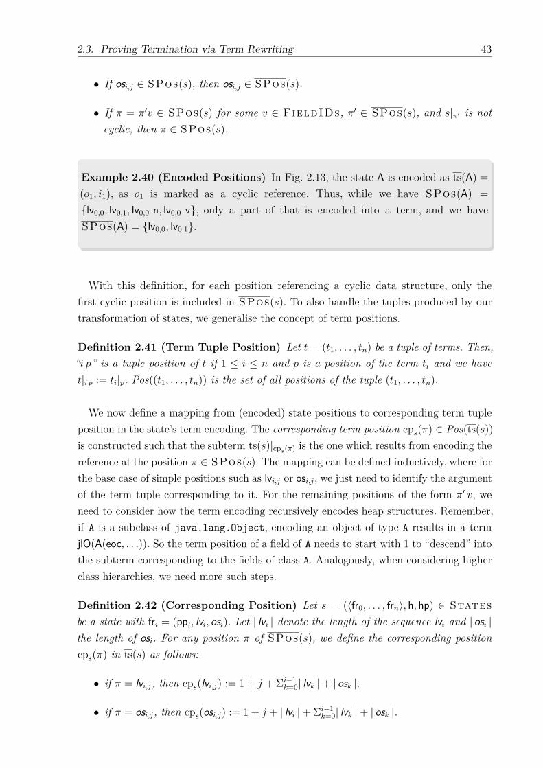
2.3. Proving Termination via Term Rewriting 43
• If osi,j ∈ SPos(s), then osi,j ∈ SPos(s).
• If π = π′v ∈ SPos(s) for some v ∈ FieldIDs, π′ ∈ SPos(s), and s|π′ is notcyclic, then π ∈ SPos(s).
Example 2.40 (Encoded Positions) In Fig. 2.13, the state A is encoded as ts(A) =(o1, i1), as o1 is marked as a cyclic reference. Thus, while we have SPos(A) ={lv0,0, lv0,1, lv0,0 n, lv0,0 v}, only a part of that is encoded into a term, and we haveSPos(A) = {lv0,0, lv0,1}.
With this definition, for each position referencing a cyclic data structure, only thefirst cyclic position is included in SPos(s). To also handle the tuples produced by ourtransformation of states, we generalise the concept of term positions.
Definition 2.41 (Term Tuple Position) Let t = (t1, . . . , tn) be a tuple of terms. Then,“i p” is a tuple position of t if 1 ≤ i ≤ n and p is a position of the term ti and we havet|i p := ti|p. Pos((t1, . . . , tn)) is the set of all positions of the tuple (t1, . . . , tn).
We now define a mapping from (encoded) state positions to corresponding term tupleposition in the state’s term encoding. The corresponding term position cps(π) ∈ Pos(ts(s))is constructed such that the subterm ts(s)|cps(π) is the one which results from encoding thereference at the position π ∈ SPos(s). The mapping can be defined inductively, where forthe base case of simple positions such as lvi,j or osi,j, we just need to identify the argumentof the term tuple corresponding to it. For the remaining positions of the form π′ v, weneed to consider how the term encoding recursively encodes heap structures. Remember,if A is a subclass of java.lang.Object, encoding an object of type A results in a termjlO(A(eoc, . . .)). So the term position of a field of A needs to start with 1 to “descend” intothe subterm corresponding to the fields of class A. Analogously, when considering higherclass hierarchies, we need more such steps.
Definition 2.42 (Corresponding Position) Let s = (〈fr0, . . . , frn〉, h, hp) ∈ Statesbe a state with fri = (ppi, lvi, osi). Let | lvi | denote the length of the sequence lvi and | osi |the length of osi. For any position π of SPos(s), we define the corresponding positioncps(π) in ts(s) as follows:
• if π = lvi,j, then cps(lvi,j) := 1 + j + Σi−1k=0| lvk |+ | osk |.
• if π = osi,j, then cps(osi,j) := 1 + j + | lvi |+ Σi−1k=0| lvk |+ | osk |.

44 Chapter 2. Termination Analysis of Java Bytecode Programs
• if π = π′ v for some v ∈ FieldIDs, then let Cl be the class in which v is defined.Furthermore let (Cl0 = java.lang.Object, Cl1, . . . , Cln = Cl) be the sequence ofclasses such that Cli is the direct superclass of Cli+1. Finally let m be the numberof the field described by v in Cl according to the order used in Def. 2.32. Then wedefine cps(π) := cps(π′) 1n (m+ 1).
Example 2.43 We continue Ex. 2.34 and consider state D in Fig. 2.11 withthe term encoding tD = fD(jlO(List(eoc, o3, i2)), i1, jlO(List(eoc, o3, i2))). The posi-tions of D are the same as the encoded positions, i.e., we have SPos(D) ={lv0,0, lv0,0 n, lv0,1, os0,0, os0,0 n} = SPos(D).For the state position π = os0,0 n, we obtain the term tuple position p = cpD(π) =
cps(os0,0) 11 (1 + 1) = (1 + 0 + 2) 1 (1 + 1) = 3 1 2. Here, the class hierarchy for the field nis java.lang.Object, List, i.e., n from Def. 2.42 is 1. Furthermore, m is 1, as n is thefirst encoded field of List. As we can see, tD|p = o3 = D|π holds, i.e., the correspondingposition of π points to the encoding of π in the state encoding of s.
We now prove the correspondence demonstrated in Ex. 2.43. Thus, for a term encodingts(s) of a state s we have that for every encoded position π ∈ SPos(s), the term encodingof the reference s|π is the same as the subterm at the corresponding term position of π,i.e., the equality ts(s)|cps(π) = tr(s, s|π) holds.
Lemma 2.44 (“Soundness” of Corresponding Position) Let s ∈ States andlet π ∈ SPos(s). Then we have ts(s)|cps(π) = tr(s, s|π).
Proof. We prove this lemma by induction over π. In the base case π is either lvi,j or osi,j,and the lemma obviously holds.Let now π = π′ v for some v ∈ FieldIDs, Cl be the class in which v is defined and
m be the number of the field described by v in Cl according to the order used in Def. 2.32Let furthermore (Cl0 = java.lang.Object, Cl1, . . . , Cln = Cl) be the sequence of classessuch that Cli is the direct superclass of Cli+1. Then we have cps(π) = cps(π′) 1n (m+ 1).Furthermore we have that tr(s, s|π′) = Cl0(Cl1(. . . (Cln(t, t1, . . . , t`), . . . ))) holds for
some terms t, t1, . . . , t` where ` ≥ m by definition of tr and because we know that s|π′ is notcyclic (as its successor π is in SPos(s)). Hence we have tr(s, s|π′)|1n(m+1) = tm = tr(s, s|π)because of the definition of tr. The induction hypothesis implies tr(s, s|π′) = ts(s)|cps(π′)
and hence tr(s, s|π) = tr(s, s|π′)|1n(m+1) = (ts(s)|cps(π′))|1n(m+1) = ts(s)|cps(π) holds by thedefinition of cps. �

2.3. Proving Termination via Term Rewriting 45
The map cps provides a term position for every encoded state position, but it is notsurjective. This is due to our term encoding, in which a non-trivial object results in severalsubterms corresponding to a single reference. In such cases, we create one subterm for eachelement of the class hierarchy, and hence, several term positions correspond to a singleposition in the state.
Example 2.45 We continue Ex. 2.43 and consider state D in Fig. 2.11 with the termencoding tD = fD(jlO(List(eoc, o3, i2)), i1, jlO(List(eoc, o3, i2))). There is no π ∈ SPos(D)with cps(π) = 1 1 or cps(π) = 1 1 1, i.e., we cannot address the subterms List(eoc, o3, i2)and eoc at the positions 1 1 and 1 1 1 of ts(D,D). These positions are induced by the termencoding of lv0,0, but are only a fragment of the term encoding for a single reference.
To handle such cases, we define the set of corresponding suffixes, which we can appendto corresponding positions to address additional subterms introduced by the translation.
Definition 2.46 (Corresponding Suffixes) Let s = (cs, h, hp) ∈ States and π ∈SPos(s). Then we define cps(π) as follows.
• If s|π = null, or s|π is cyclic, or h(s|π) /∈ Instances, then we define cps(π) :={ε}.
• Otherwise let h(s|π) = (Cl, f), and let (Cl0 = java.lang.Object, Cl1, . . . , Cln = Cl)be the sequence of classes such that Cli is the direct superclass of Cli+1. Then wedefine cps(π) := {ε, 1, . . . , 1n+1}.
Example 2.47 We continue Ex. 2.45 and consider state D in Fig. 2.11. To address allsubterms of the term encoding ts(D,D), we can now use a concatenation of positionsin cp and the suffixes from cp. So, using cpD(lv0,0) = 1 as prefix and the elementsof cps(lv0,0) = {1, 1 1} as suffixes, we can now construct 1 1 and 1 1 1, addressing thesubterms List(eoc, o3, i2) and eoc respectively.Note that 1 1 2 cannot be constructed from the corresponding position of lv0,0 and
its suffixes, as we have cpD(lv0,0 n) = 1 1 2. This is intended, as 1 1 2 corresponds to theterm encoding of the reference o3, whereas 1 1 1 is part of the encoding of the referenceo1 = D|lv0,0 .
Together, cp and cp can address every position in the tuple of terms resulting from thetransformation of a state.

46 Chapter 2. Termination Analysis of Java Bytecode Programs
Lemma 2.48 Let s ∈ States. Then Pos(ts(s)) = {cps(π) p | π ∈ SPos(s), p ∈cps(π)}.
Proof. This follows trivially from the definitions of ti, cp and cp. �
We now connect these relationships between state and term positions to the notion ofinstances. Just as s′ v s means that all state positions of s also exist in s′, we can concludea similar relationship for the positions in their respective term encodings.
Lemma 2.49 (Instance and Corresponding Positions) Let s, s′ ∈ States withs′ v s and let π ∈ SPos(s). Then we have cps(π) = cps′(π) and cps(π) ⊆ cps′(π).
Proof. First note that π ∈ SPos(s) implies π ∈ SPos(s′) by Lemma 2.37, and similarly,π ∈ SPos(s) also implies π ∈ SPos(s′). From this, we can conclude the first part of theproposition, as cps(π) depends only on the number of local variables and operand stackentries in a state and the class hierarchy, which is fixed for one considered program.The claim cps(π) ⊆ cps′(π) follows trivially from s′ v s. �
In a last step, we show that if s′ is an instance of s and the same variable r occurs attwo different positions p and p′ in the term encoding of s, then the subterms at thesepositions in the encoding of s′ are also identical. The reason for this is that variables interm encodings correspond to references in the respective states, and hence, equal variablesmean equal references. At the same time, the definition of v ensures that references thatare equal in the more abstract state s are also equal in s′.
Lemma 2.50 Let s, s′ ∈ States with s′ v s and let ts(s)|p = ts(s)|p′ ∈ Refs. Thenwe also have ts(s′)|p = ts(s′)|p′.
Proof. Because of ts(s)|p = r ∈ Refs, we have ts(s)|p = tr(s, r). Let π ∈ SPos(s) besuch that cps(π) q = p for a q ∈ cps(π). Such π and q must exist by Lemma 2.48. Thenwe have q = ε because of the definitions of cp and tr. Analogously, let π′ ∈ SPos(s) besuch that cps(π′) = p′.Now we have r = ts(s)|p = ts(s)|cps(π) = tr(s, s|π) and hence s|π = r. Analogously
we have s|π′ = r. Hence π and π′ address the same reference in s, i.e., we have s|π =s|π′ . Because s′ is an instance of s we also have s′|π = s′|π′ . By Lemma 2.49, we havep = cps(π) = cps′(π) and p′ = cps(π′) = cps′(π′). As π and π′ also address the samereference in s′, by Lemma 2.44 we have ts(s′)|p = ts(s′)|cps′ (π) = tr(s′, s′|π) = tr(s′, s′|π′) =ts(s′)|cps′ (π′) = ts(s′)|p′ . �

2.3. Proving Termination via Term Rewriting 47
Example 2.51 As in Ex. 2.36, we consider states B and D from Fig. 2.11. We haveD v B and
ts(B,B) = fB(o1, i1, o1)
ts(D,B) = fB(List(eoc, o3, i2), i1, List(eoc, o3, i2))
So we have ts(B,B)|1 = ts(B,B)|3 = o1 ∈ Refs. In D, o1 was replaced everywhere by o2,which points to list element, and consequently, ts(D,B)|1 = ts(D,B)|3 = List(eoc, o3, i2)holds.
Finally, we can combine these lemmas to prove Lemma 2.35, showing that if s′ v s,there is some substitution σ such that ts(s′) = ts(s)σ.
Proof. (Proof of Lemma 2.35) Let s = (cs, h, hp) and s′ = (cs′, h′, hp′) Moreover, let π ∈SPos(s) with s|π = r ∈ Refs. Since s′ v s, by Lemma 2.37, (resp. by its extension toencoded positions) we also have π ∈ SPos(s′). Hence, there exists a reference r′ withr′ = s′|π. We will now show that the term representation of r in s matches the termrepresentation of r′ in s′. In other words, there is a substitution σr = [r/t] such thattr(s, r)σr = tr(s′, r′).
In Lemma 2.50, we showed that if the same variable r occurs at two different positionsp and p′ in the tuple of terms ts(s), then the terms at the positions p and p′ in the tupleof terms ts(s′) are also identical. Hence, the different substitutions σr for the differentreferences r above can be combined into one single substitution σ satisfying ts(s)σ = ts(s′).To prove the existence of a substitution σr with tr(s, r)σr = tr(s′, r′), we perform
induction on the term structure of tr(s, r).If tr(s, r) = i ∈ Z, then h(r) = h(s|π) = [i, i] ∈ Integers. As s′ v s, we also have
h′(s′|π) = [i, i]. Hence, tr(s′, r′) = i = tr(s, r) and thus, σr is the identity.If tr(s, r) = null, then r = s|π = null. Hence s′ v s implies r′ = s′|π = null as well. So
tr(s′, r′) = null = tr(s, r) and thus, σr is again the identity.If tr(s, r) is the variable r, then we simply let σr be the substitution that instantiates
the variable r by the term tr(s′, r′).Finally, we regard the case where h(r) ∈ Instances, and thus,
tr(s, r) = ti(s, r) = Cl0(Cl1(. . . (Cln(eoc, vn,1, . . . , vn,mn), . . . ), v1,1, . . . , v1,m1))
(Note that the class Cl0 = java.lang.Object has no fields.) As h(r) = h(s|π) ∈Instances and s′ v s holds, we have that h′(r′) = h′(s′|π) ∈ Instances as welland the types of h(r) and h′(r′) are equal.

48 Chapter 2. Termination Analysis of Java Bytecode Programs
Thus,
tr(s′, r′) = ti(s′, r′) = Cl0(Cl1(. . . (Cln(eoc, v′n,1, . . . , v′n,mn), . . . ), v′1,1, . . . , v′1,m1)).
Let pi,j be the position of vi,j in ts(s) and of v′i,j in ts(s′), and let πi,j ∈ SPos(s) besuch that pi,j = cps(πi,j). So for πi,j we have s|πi,j = ri,j such that vi,j = tr(s, ri,j) byLemma 2.44.
By Lemma 2.49, cps(πi,j) = cps′(πi,j) = pi,j, and hence v′i,j = tr(s′, s′|πi,j) by Lemma 2.44.Hence, by the induction hypothesis there is a substitution σri,j such that vi,jσri,j = v′i,j.As discussed above, by Lemma 2.50 the different substitutions σri,j can be combined
into one single substitution σr satisfying vi,jσr = v′i,j for all i, j. This implies tr(s, r)σr =tr(s′, r′). �
2.3.3 Transforming Termination Graphs
We now extend our transformation of states to terms to a transformation of edges intermination graphs to term rewrite rules. Our goal is to create rules that allow a rewritestep on the term encoding of a state whenever the original program can be evaluated onthat state. Then, if no rewrite steps are possible, further evaluation of the program is notpossible, and consequently, termination of the generated rules implies termination of theresulting program.
To this end, we use one symbol for each state in our termination graph. The argumentsto this symbol are the tuple of term encodings as defined above in Def. 2.33. We thendefine a translation function rule(s, l, s′) to map an edge e between two states s and s′
with a label l to a rewrite rule. In the most simple case, if e corresponds to a normalevaluation step and hence, the label ` is Eval∅, and we create a rule ts(s, s)→ ts(s′, s′).By Lemma 2.50, we know that for every concrete state c v s, there is a substitution σsuch that ts(c, s) = ts(s, s)σ, and hence, we can apply the rule on ts(c, s). In this way, ourrewrite rules are based on the termination graph, but apply to any concrete evaluation.
Example 2.52 (Evaluation Simulated by Term Rewriting) We again considerthe termination graph for get in Fig. 2.13. In the following, we will discuss how toautomatically obtain the rule fB(o1, i1, o1) → fC(o1, i3, o1, i1) J i3 = i1 − 1 K for the eval-uation edge between B and C. In a concrete evaluation in which we want to get thesecond list element, we could for example obtain a state B′ v B with the term encodingt = fB(o′1, 2, o′1) (remember, the considered list has to be cyclic and thus, its term encod-ing is always just a variable). Rewriting t with our rule yields the term fC(o′1, 1, o′1, 2),matching the method get, in which we decrement the variable x at the start of the loop.

2.3. Proving Termination via Term Rewriting 49
a1 a2 a3 a4 a5 . . .
c1 c2 c5 . . .
t1 t2 t3 t4 t5 . . .
Eval Ins Refine Eval
Eval Eval
↪→rule((a1,Eval,a2)) ↪→rule((a2,Ins,a3)) ↪→rule((a3,Refine,a4)) ↪→rule((a4,Eval,a5))
v vv
vv
ts ts ts
Figure 2.14: Relation between concrete computation sequences, paths in the terminationgraph and the generated rewrite rules
This relation is displayed in Fig. 2.14, where the states c1, c2, and c5 correspond toa sequence of concrete states obtained by evaluation. The states a1, a2, . . . , an are thesequence of states in the termination graph that represent the evaluation (which haveto exist by Thm. 2.23). By transforming each of the edges in the graph to rewrite rules,we can then emulate the computation on the term rewrite level, and thus have a rewritesequence t1 ↪→ t2 ↪→ . . . ↪→ tn, where each term ti corresponds to an abstract state ai inthe graph.We can translate almost all evaluation edges of the form (s,EvalC , s′) to the rule
ts(s, s) → ts(s′, s′) J tc(C) K, where the mapping tc(C) just transforms the set of integerarithmetic operations and relations on the edge into a conjunction of these constraints.However, this does not hold for edges encoding a putfield instruction, i.e., those on whicha write access to an object instance happens. For such evaluations, we need to take intoaccount that sharing effects are not represented completely by our term representation.Consequently, if we have an evaluation step in which some reference r that may sharewith another reference r′ is changed by a write access, our rewrite system cannot easilyrepresent the effect of this change on r. To solve this problem, we use a fresh variableinstead of the term encoding of r′ on the right-hand side of our rule. This fresh variable canthen be instantiated by any term, including the one that matches the actual change. So ingeneral, we encode evaluation edges from state s to state s′ as ts(s, s)→ ts(s′, s′) J tc(C) K,where ts usually behaves like ts. Only if the evaluation edge represents a write access tor′, ts encodes all occurrences of references r with r %$ r′ by a fresh variable.
Example 2.53 (Translation of EvalC Edges) Consider the edge between G and Hin Fig. 2.11, which is encoded as the rule
fG(jlO(List(eoc, o3, i2)), i1, i1, i2)→ fH(o3, i1) J i1 6= i2 K
Note that the edge between G and H actually corresponds to several evaluation steps.However, to illustrate our translation, we handle this as one step and in general, a

50 Chapter 2. Termination Analysis of Java Bytecode Programs
sequence of evaluation steps could be encoded into one rule.
The translation of refinement edges, i.e., cases with ` = RefineR is very similar. Asfollowing a refinement edge corresponds to choosing a case in a case analysis, we canassume that all additional information we obtain in the refined state already held in theoriginal state (if it does not, we can use a rule obtained from the edges correspondingto the alternative cases instead). Hence, we transform refinement edges from state s tostate s′ as ts(s′, s) → ts(s′, s′), using the more refined term encoding of s′ (as it is moreconcrete) also on the left-hand side of the rule, but using s as label for the defined symbol.
Example 2.54 (Translation of RefineR Edges) Consider the edges from B to Cand D in Fig. 2.11. Any concrete state represented by B is represented by one of therefinement successors C and D (cf. Def. 2.14), so its term encoding has to be an instanceof the term encoding of C or D. Consequently, we encode the two edges as follows.
fB(null, i1, null)→ fC(null, i1, null)
fB(jlO(List(eoc, o3, i2)), i1, jlO(List(eoc, o3, i2)))→
fD(jlO(List(eoc, o3, i2)), i1, jlO(List(eoc, o3, i2)))
Finally, when we are encoding an instance edge, the situation is reversed. Here, thesource state contains more concrete information than the target state. Hence, we encodeinstance edges as ts(s, s)→ ts(s, s′).
Example 2.55 (Translation of Ins Edges) Consider the edges from B to G, F to Gand O to G in Fig. 2.13. The state G is more abstract than both B and F, which bothcontain definite information about the connection between this and cur. On the otherhand, O is just a variable renaming of G. We obtain the following three rules:
fB(jlO(List(eoc, o2, i2)), i1, jlO(List(eoc, o2, i2)))→
fG(jlO(List(eoc, o2, i2)), i1, jlO(List(eoc, o2, i2)))
fF(jlO(List(eoc, o2, i2)), i3, o2)→
fG(jlO(List(eoc, o2, i2)), i3, o2)
fO(jlO(List(eoc, o2, i2)), i3, o5)→
fG(jlO(List(eoc, o2, i2)), i3, o5)

2.3. Proving Termination via Term Rewriting 51
Definition 2.56 (int-rewrite Rules From Termination Graphs) Let G = (V,E) bea termination graph, and e = (s, `, s′) ∈ E an edge in G with s = (cs, h, hp). We definethe corresponding rule rule(e):
• if ` = Ins, then rule(e) := ts(s, s)→ ts(s, s′).
• if ` = RefineR, then rule(e) := ts(s′, s)→ ts(s′, s′).
• if ` = EvalC, then rule(e) := ts(s, s) → ts(s′, s′) J tc(C) K, where ts is like ts, butif the edge represents a write access to some reference r, ts encodes all occurrencesof references r′ with r %$ r′ by a fresh variable.
Finally, we define the int-rewrite system corresponding to G as rules(G) := {rule(e) | G =(V,E), e ∈ E}.
Based on this, we can now transform all edges in our termination graphs to a rewritesystem simulating the original program. However, not all rewrite sequences correspondto valid programs runs. There are two reasons for this. One is the missing informationabout the start of computations. Whereas a program has a clearly defined start, a rewritesequence can start in any term, representing any state. The second difference is due toour representation of sharing effects and cyclicity, which we only approximate in our termencoding. The most important consequence is that non-termination proofs for the resultingterm rewrite system do not allow to conclude non-termination of the original program.
Example 2.57 If G is the graph from Fig. 2.11, rules(G) results in the following rules:
fA(o1, i1)→ fB(o1, i1, o1)
fB(null, i1, null)→ fC(null, i1, null)
fC(null, i1, null)→ fCe()
fB(jlO(List(eoc, o3, i2)), i1, jlO(List(eoc, o3, i2)))→
fD(jlO(List(eoc, o3, i2)), i1, jlO(List(eoc, o3, i2)))
fD(jlO(List(eoc, o3, i2)), i1, jlO(List(eoc, o3, i2)))→ fE(jlO(List(eoc, o3, i2)), i1, i1, i2)
fE(jlO(List(eoc, o3, i2)), i1, i1, i1)→ fF(jlO(List(eoc, o3, i1)), i1, i1, i1)
fF(jlO(List(eoc, o3, i1)), i1, i1, i1)→ fFe()
fE(jlO(List(eoc, o3, i2)), i1, i1, i2)→ fG(jlO(List(eoc, o3, i2)), i1, i1, i2)
fG(jlO(List(eoc, o3, i2)), i1, i1, i2)→ fH(o3, i1) J i1 6= i2 K
fH(o3, i1)→ fI(o3, i1)
fI(o3, i1)→ fA(o3, i1)

52 Chapter 2. Termination Analysis of Java Bytecode Programs
Our second soundness theorem now states that the transformation of termination graphsto TRSs discussed above indeed suffices to prove termination graphs well-founded:
Theorem 2.58 Let G be a termination graph. If rules(G) is terminating, G is well-founded.
We prove this below, as we again first need to introduce some additional lemmas, butwe can already combine Thm. 2.23 and Thm. 2.58 to conclude the overall soundness ofour termination analysis approach:
Corollary 2.59 Let P be some program and G a termination graph for P . If rules(G)is terminating, then P is terminating.
Proof. If rules(G) is terminating, then Thm. 2.58 implies that G is well-founded. Further-more, Def. 2.24 implies that all evaluations represented by G are then also finite. At thesame time, Thm. 2.23 implies that all possible evaluations of P are represented by G, andhence, all evaluations of P are terminating. �
We now prove Thm. 2.58 by a case analysis, considering each edge type on its own. Ina first step, we consider the case of an evaluation edge. We prove that the rule obtainedfor the evaluation edge indeed rewrites the term encoding of a represented concrete stateinto the term encoding of its evaluation successor.
Lemma 2.60 (Correctness of rule(e) for Evaluation Edges) Let G = (V,E) bea termination graph with (s,EvalC , s′) = e ∈ E. Let c be a concrete state with c v s
and let c′ result from c by a single JBC evaluation step. Then we have ts(c, s) ↪→rule(e)
ts(c′, s′).
Proof. Let rule(e) = `→ r Jϕ K. By Lemma 2.35, there exists a substitution σ such that`σ = ts(s, s)σ = ts(c, s). We will now show that σ can be extended to σ such that `σ = `σ,rσ = ts(c′, s′), and ϕσ is valid.For this, we consider the term encoding of ts(c′, s′), for which, by Lemma 2.35, there
exists some substitution ν such that ts(c′, s′) = ts(s′, s′)ν = rν. We now define
σ(x) :=
σ(x) if x is a variable in `
ν(x) if x is a variable not in `, but in r
c otherwise, where c is chosen such that ϕ is valid

2.3. Proving Termination via Term Rewriting 53
This correctly instantiates free variables caused by write accesses (cf. Def. 2.56). Obviously,`σ = ts(c, s) holds, and what remains is to show rσ = ts(c′, s′). For this, we show thatν(x) = σ(x) for all x that also occur in `. As x occurs in `, the reference x is reachablein the state s and x 6= null. Note that since x occurs both in ` and r, it was not sharingwith any possible write access (otherwise, it would have been replaced by a free variable).Hence, the heaps of s and s′ do not differ at the address x, and analogously, the heaps ofc and c′ do not differ either. Thus, σ(x) = ν(x) and consequently, rσ(x) = ts(c′, s′).
As a concrete evaluation step from c to c′ was possible, there is a satisfying assignmentfor the variables in ϕ. For those variables occurring in ` or r, we have already chosenthe corresponding values from the satisfying assignment. For the remaining variables onlyoccurring in ϕ, σ is constructed such that ϕ is satisfied. Hence, ϕσ is valid, and a rewritestep with rule(e) is allowed. �
We can now lift this result from single evaluation edges to sequences of edges, whichmay also include refinement (concretisation) and instance (abstraction) steps.
Lemma 2.61 (Simulation of Concrete Evaluations by rules(G)) LetG = (V,E) be a termination graph with s ∈ V and c ∈ States be a concretestate with c v s. Let c′ result from c by a single JBC evaluation step. By Thm. 2.23there is a successor s′ ∈ V with s
(Ins−→ ∪ Refine−→
)∗◦ Eval−→ s′ in G such that c′ v s′.
Then, ts(c, s) ↪→+rules(G) ts(c′, s′).
Proof. Let the path between s and s′ be s = s0, s1, . . . , sn = s′ such that `i is the label ofthe edge between si−1 and si. By Thm. 2.23, `n is EvalC and all `i with 1 ≤ i < n− 1are either RefineR or Ins, and we have c v s0, . . . , c v sn−1.
We now prove the proposition by induction over the length n of the path between s ands′. In the base case, we have n = 1, `1 = EvalC , and by Lemma 2.60, ts(c, s) ↪→+
rule((s,`1,s′))
ts(c′, s′) holds.In the induction step, let n > 1. By our induction hypothesis, we have ts(c, s1) ↪→+
rules(G)
ts(c′, s′). We now prove that ts(c, s0) ↪→rule((s0,`1,s1)) ts(c, s1) holds, and combine this withthe induction hypothesis to obtain ts(c, s0) ↪→+
rules(G) ts(c′, s′). By construction of our pathfrom s to s′, `1 is either Ins or RefineR.
If `1 = Ins, then rule((s0, `1, s1)) is just ts(s0, s0)→ ts(s0, s1). As c v s0, by Lemma 2.35,there is some substitution σ with ts(s0, s0)σ = ts(c, s0). Hence, by using σ in the rewriterelation, we get ts(c, s0) ↪→σ
rule((s0,Ins,s1))→ ts(c, s1).If `1 = RefineR, then rule((s0, `1, s1)) is just ts(s1, s0) → ts(s1, s1). As c v s1, by
Lemma 2.35, there is some substitution σ with ts(s1, s1)σ = ts(c, s1). Hence, by using σin the rewrite relation, we get ts(c, s0) ↪→σ
rule((s0,RefineR,s1))→ ts(c, s1). �

54 Chapter 2. Termination Analysis of Java Bytecode Programs
Based on this lemma about the simulation of single evaluation steps in the resultingint-TRS, we can now finally prove Thm. 2.58.
Proof. (Proof of Theorem 2.58) We prove the theorem by contradiction. Assume rules(G)is terminating, and let G = (V,E) be a termination graph that is not well-founded, i.e.,there is a concrete state c ∈ States with c v s ∈ V and an infinite computationstarting in c. Consequently, there is an infinite sequence of states c = c1, c2, c3, . . . suchthat ci+1 is obtained from ci by evaluation. By Thm. 2.23, there is a corresponding sequences1, s2, s3, . . . of states from G, such that si
(Ins−→ ∪ Refine−→
)∗◦ Eval−→ si+1 and ci v si holds.
Then, by Lemma 2.61, we can simulate each of these steps in rules(G), i.e., we havets(ci, si) ↪→+
rules(G) ts(ci+1, si+1). As c1, c2, . . . is an infinite sequence, the correspondingsequence of term encodings is an infinite reduction in rules(G), and hence, rules(G) is notterminating. �

2.4. Post-processing Termination Graphs 55
2.4 Post-processing Termination Graphs
In the basic termination analysis presented above, we directly transform a terminationgraph into a term rewrite system. However, to strengthen our analysis and allow it tohandle more complex problems, we have developed a number of techniques that workdirectly on the termination graph and provide data that can be used to obtain a moreprecise term encoding. The first set of techniques is presented in Sect. 2.4.1 and allows togreatly simplify the resulting term rewrite systems. In many cases, these techniques evenallow to prove termination of programs that work with cyclic data structures. However,these techniques do not allow to prove termination of algorithms that only terminatebecause the used data structures are cyclic. In Sect. 2.4.2, we introduce a technique thatcan be used to prove termination of algorithms that “mark” visited elements, and terminatewhen no unmarked elements remain. Finally, in Sect. 2.4.3, we handle examples that onlyterminate because a data structure is cyclic, i.e., list iterations that continue until reachingthe first element again.
2.4.1 Optimisations of the Term Transformation
The transformation of termination graphs to int-TRSs defined in Def. 2.56 provides thebasis for termination analysis of JBC programs. In the implementation of our approach,a number of additional optimisations were added to make the technique more efficient andallow for the analysis of larger programs.
In a first step, we can split the termination analysis of the resulting term rewrite systemsinto smaller parts. For this, we use the observation that a non-terminating computationhas to eventually stay in one strongly connected component (SCC) of the program, andhence, it is enough to prove every SCC terminating on its own.14 Hence, we use a simplegraph analysis on the termination graph to identify its SCCs, and then encode each SCCinto a separate int-TRS that is then analysed on its own. This reduces the size of theconsidered problems, and allows to easily parallelise their analysis.
In a second step, we simplify the representation of states as terms. For this, we computewhich references are influencing the control flow in the encoded part of the graph. Dueto renamings in refinements, such references may be different from state to state. Hence,we compute a set of interesting references IRefss for each state s. As our symbolicevaluation is deterministic, it suffices to consider those references that lead to a refinement.Hence, for refinement edges (s,RefineR, s′), we require R ⊆ IRefss. Furthermore, wepropagate interesting references backwards, i.e., if r is marked as interesting in some state14 Note that the precision of the overall method does not suffer from this. As we use term rewriting as
back-end, we do not consider start states and hence, every term (“configuration”) can serve as thestart of a reduction. In other formalisms that consider start terms (e.g., the integer transition systemspresented in Chapter 4), this simplification would lose precision.

56 Chapter 2. Termination Analysis of Java Bytecode Programs
s, and some other reference r′ “contributes” to r in some predecessor s′, we mark r′ asinteresting in s′. Here, “contribute” can mean that r is r′, or that the edge between s′ ands is marked by an expression like r = r′ + 1.
Example 2.62 (Interesting References in Fig. 2.13) We compute the interestingreferences for the only SCC S of Fig. 2.13, made up by the nodes G, H, J, K, L, M, N, O,P and their connecting edges.Based on the existing refinement edges, we initialise IRefsH to {i3}, IRefsK to{o1, o3} and IRefsL to {o3}. We then propagate the information backwards, untilreaching a fixed point. So because i3 is in IRefsH , we also add i3 to IRefsG , as Gis a predecessor of H. Then, we also add i6 to IRefsO , because O has an Ins edgeto G, and i6 is the reference that appears in O at the positions of i3 in G. Similarly, wecontinue for all other edges and states, until reaching a fixpoint with the following setsof interesting references:
IRefsG = {i3, o1, o3} IRefsH = {i3, i6, o1, o3} IRefsJ = {i8, i6, o1, o3}
IRefsK = {i6, o1, o3} IRefsL = {i6, o1, o3} IRefsN = {i6, o1, o5}
IRefsO = {i6, o1, o5} IRefsM = {i6, o1} IRefsP = {i6, o1, o2}
While these are the relevant references that are needed to determine decisions aboutthe control flow, it does not suffice to encode just these reference. As example, considerthe reference o5 ∈ IRefsN , which is only reachable through the object referenced byo4. Hence, we also add references that point to an object from which we can reach aninteresting reference by following some fields. So if we have an interesting reference r in astate s at position s|π, then all references at prefixes τ ∈ SPos(s) of π are relevant forthe term encoding, and we construct the set IRefss from them.
Example 2.63 (Interesting References in Fig. 2.13) For the graph from Fig. 2.13,we obtain the following references that are interesting for the term encoding:
IRefsG = {i3, o1, o3} IRefsH = {i3, i6, o1, o3} IRefsJ = {i8, i6, o1, o3}IRefsK = {i6, o1, o3} IRefsL = {i6, o1, o3} IRefsN = {i6, o1, o4, o5}IRefsO = {i6, o1, o5} IRefsM = {i6, o1} IRefsP = {i6, o1, o2}
Definition 2.64 (Interesting References) Let G = (V,E) be a termination graph, andlet S ⊆ V be an SCC of G. Let G′ = (S, E ′) be the subgraph induced by S, with edges

2.4. Post-processing Termination Graphs 57
class DList {DList prev;DList next;static int length(DList x) {
int r = 0;while (x != null) {
x = x.next;r++;
}return r;
}}
(a) Java program
00: iconst_0 #load 001: istore_1 #store to r02: aload_0 #load x03: ifnull 17 #jump if
# x null06: aload_0 #load x07: getfield next #read x.next10: astore_0 #store to x11: iinc 1, 1 # increment r14: goto 0217: iload_1 #load r18: ireturn #return r
(b) JBC for length
Figure 2.15: length computation on doubly linked list
E ′ = {(s, `, s′) ∈ E | s, s′ ∈ S}. Then IRefsS(s) ⊆ SRefs(s)} is the set of interestingreferences of s in S, defined as the minimal set of references with
• if (s,RefineR, s′) ∈ E ′, then R ⊆ IRefsS(s).
• if (s, l, s′) ∈ E ′ with l ∈ {RefineR, Ins}, then we have {s|π | π ∈ SPos(s) ∩SPos(s′), s′|π ∈ IRefsS(s′)} ⊆ IRefsS(s).
• if (s,EvalC , s′) ∈ E ′, then IRefsS(s′) ∩ {s|π | π ∈ SPos(s)} ⊆ IRefsS(s).
• if (s,EvalC , s′) ∈ E ′, i = i′ ./ i′′ ∈ C and i ∈ IRefsS(s′), then {i′, i′′} ⊆IRefsS(s).
Finally, we define the set of interesting term encoding references of s as IRefsSs =
{s|τ | π, τ ∈ SPos(s), s|π ∈ IRefsS(s), τ prefix of π}.
We will use the set IRefss to restrict our term encoding ts of states to those referenceswe need for a termination proof, greatly reducing the number of variables and constraintsin the resulting term rewrite system. However, we can do even better and finally makeuse of the detailed information we keep in the cyclicity heap predicate F . As example,consider the program in Fig. 2.15, which introduces a class DList with fields next andprev that can be used to construct a doubly linked list (as in Fig. 2.10). The methodlength then computes the length of such a list by following the next pointer until reachingthe end of the list. This method only terminates on lists without cycles that only use thenext field, displayed on the left of Fig. 2.10.A termination graph for the method in Fig. 2.15 is displayed in Fig. 2.16. There, we
abbreviate the class name DList as DL and the field names next (resp. prev) as n (resp.p). We start with state A, representing all cases of calling the method on a list in whichall cycles use both next and prev fields. Between A and B, the variable r is initialised to

58 Chapter 2. Termination Analysis of Java Bytecode Programs
00 |x :o1 |εo1:DL(?) o1 {p,n}
A
02 |x :o1, r :0 |εo1:DL(?) o1 {p,n}
B
03 |x :o1, r :0 |o1
o1:DL(?) o1 {p,n}
C
03 |x :null, r :0 |null D 03 |x :o2, r :0 |o2
o2:DL(p=o3, n=o4)o3:DL(?) o4:DL(?)o2%$o3 o2%$o4 o3%$o4o2, o3, o4 {p,n}
E
02 |x :o4, r :1 |εo4:DL(?) o4 {p,n}
F
02 |x :o5, r : i1 |εo5:DL(?) o5 {p,n} i1: [≥0]
G
03 |x :o5, r : i1 |o5
o5:DL(?) o5 {p,n} i1: [≥0]
H
03 |x :null, r : i1 |nulli1: [≥0]
I
03 |x :o6, r : i1 |o6
o6:DL(p=o7, n=o8)o7:DL(?) o8:DL(?)o6%$o7 o6%$o8 o7%$o8o6, o7, o8 {p,n} i1: [≥0]
J02 |x :o8, r : i2 |εo8:DL(?) o8 {p,n} i2: [≥1]
K
1 = 0 + 1
i2 = i1 + 1
Figure 2.16: Termination Graph for length
0. Evaluation then continues to C, where the value of x (o1) is tested for equality to null.We perform an instance refinement, yielding states D and E. From D, further evaluationleads to a return statement. In E, we have replaced o1 by a new reference o2, resolvedto a DList object instance with fields prev and next. These fields in turn contain freshreferences o3 and o4 that share with o2, and carry the same cyclicity information. Symbolicevaluation from E on can continue without need for further refinements until reachingstate F at program position 02. On the way, the value of r was incremented, and x wasupdated to contain the value of o2’s next field, o4.
B and F are at the same program position, but only differ in the value of r. We mergethe two states, resulting in G, where r points to any non-negative number. Symbolicevaluation from G proceeds as from B, leading to a refinement for the null check in H, toa method end in I and to another state at the same program position as G in K. Here, Kis just an instance of G, and we can draw an instance edge from K to G, completing thetermination graph.
With the translation of terms presented in Sect. 2.3.2, we cannot prove termination of themethod. The reason for this is the heap predicate {p,n} that is used to mark all occurringobjects. According to Def. 2.32, this means that all these references are transformed to justa variable of the same name, as we cannot represent cyclic objects as terms. On the otherhand, the cycles allowed in the data structure are irrelevant for the termination argumentneeded for length: In our main loop, we only ever use the next field, so as long as theinput list contains no cycles entirely made up from next fields, we can prove termination.Intuitively, the problem stems from the fact that our loop only considers the next fieldsin the data structure, and in this restricted view, it is indeed acyclic.

2.4. Post-processing Termination Graphs 59
To formalise this intuitive notion of “considered fields”, we introduce two concepts. Thefirst, interesting fields IFieldsSCl, is closely related to the interesting references fromabove. It is the set of fields of the class Cl that “lead” to an interesting reference in aincluded in some SCC S of the termination graph. Secondly, we introduce read fieldsRFieldsSCl, which are all those fields that are read somewhere in the SCC S. The twosets are often orthogonal. For example, an interesting reference may also appear in somefield f , but if the field is never read (and hence, its contents are never observed), it is notimportant for the control flow. At the same time, a read field may be of no importancebecause its value is only used to accumulate a result and not influence the control flow.Hence, the encoded fields EFieldsSCl of a class Cl combine the two sets, collecting thosefields that may contain interesting references and which are read in the SCC S.
Example 2.65 (Interesting, Read, and Encoded Fields in Fig. 2.16) We con-sider the SCC S of nodes G, H, J and K and the only class DList. In H, a refinement isperformed with respect to the reference o5, and we obtain IRefsSG = IRefsSH = {o5},IRefs SJ = {o6, o8}, and IRefs SK = {o8}. So in J, the field next contains the interestingreference o8. Hence, we obtain IFieldsSDList = {next}. Only the field next is read, andconsequently, we have RFieldsSDList = {next} and hence, EFieldsSDList = {next},too.
Definition 2.66 (Interesting, Read, and Encoded Fields) Let G = (V,E) be a ter-mination graph, and let S ⊆ V be an SCC of G. For a class Cl with fields F , we defineIFieldsSCl := {f ∈ F | ∃s ∈ S, π ∈ SPos(s).s|π f ∈ IRefsS}. Furthermore, letRFieldsSCl be the set of fields f of Cl for which the instruction getfield f is executedsomewhere in S. Finally, EFieldsSCl := IFieldsSCl ∩RFieldsSCl.
We now use the information in IRefs and EFields to refine our encoding of states.In the following, we fix an SCC S that we want to transform into a rewrite system. First,we adapt the term encoding of object instances to only encode those fields of a class Clthat are in EFieldsSCl. We also improve the encoding of possibly cyclic objects. So whenwe have the predicate r F in our state and want to encode a reference r of type Cl, wecheck if F ⊆ EFieldsSCl holds. If not, we are only encoding an acyclic projection of r,and can easily give a term encoding of it. For this, we call r definitely cyclic in a state sif there is a position π ∈ SPos(s) and a suffix τ such that s|π = s|πτ .
Definition 2.67 (Refined Term Encoding of Object Instances) We start our en-coding at the root of the class hierarchy with java.lang.Object and define ti(s, r) :=ti(s, r, java.lang.Object).

60 Chapter 2. Termination Analysis of Java Bytecode Programs
Let s = (cs, h, hp) ∈ States and let h(r) = (Clr, f) ∈ Instances. Let (Cl1 =java.lang.Object, Cl2, . . . , Cln = Clr) be ordered according to the class hierarchy, i.e.,Cli is the direct superclass of Cli+1. We define the term ti(s, r, Cli) as follows:
ti(s, r, Cli) :=
r if r is def. cyclic
r if r F∈ hp with
F ⊆ EFieldsSCli
Cli(ti(s, r, Cli+1), tr(s, f(f1)), . . . , tr(s, f(fm))) otherwise, if Cli 6= Clr
Cli(eoc, tr(s, f(f1)), . . . , tr(s, f(fm))) otherwise, if Cli = Clr
Here, let f1, . . . , fm be the fields of EFieldsSCli in some fixed order.
Furthermore, we restrict ourselves to encoding the interesting references in states, notencoding those values that do not influence the control flow.
Definition 2.68 (Refined Term Encoding of States) Let s = (〈fr0, . . . , frn〉, h, hp) ∈States be a state with fri = (ppi, lvi, osi) and let lv0 ◦ os0 ◦ lv1 ◦ os1 ◦ . . . lvn ◦ osn = r ∈Refs∗ be the concatenation of all reference lists of local variables and operand stacks.Let r1 . . . rk be those references in r which also occur in IRefsSs . We define the followingmapping from states to encodings of their references ts(s) = (tr(s, r1), . . . , tr(s, rk)) andts(s, id) = fid(ts(s)) to transform a state to a term with label id.
The proofs for the soundness of our approach can easily be adapted to these refined termencodings. In practice, these two optimisations greatly reduce the arity of the generatedterms, and allow us to use termination arguments about acyclic parts of cyclic datastructures. The advantages of this optimisation can be seen in our evaluation in Sect. 2.6.
Example 2.69 (Refined Term Encoding of Fig. 2.16) We continue Ex. 2.65 anduse the refined encodings defined in Def. 2.67 and Def. 2.68 to generate rules for theSCC S:
fG(o5)→ fH(o5, o5)
fH(DL(o8),DL(o8))→ fJ(DL(o8),DL(o8)) (2.3)
fJ(DL(o8),DL(o8))→ fK(o8)
fK(o8)→ fG(o8)
The termination argument for the method is now obvious, as (2.3), which shortens theremaining list by one element, has to be used in every cycle of the rewrite system.

2.4. Post-processing Termination Graphs 61
public class List {public GraphNode val;public List next;
}
public class GraphNode {private int mark;private Object val;private List children ;
private static void visit( GraphNode node ,int expectedMark ) {
if (node.mark == expectedMark ) {node.mark = expectedMark + 1;List curChild = node. children ;while ( curChild != null) {
GraphNode child = curChild .val;curChild = curChild .next;if (child != null) {
visit(child , expectedMark );}
}}
}}
Figure 2.17: Marking visit algorithm on a graph
Further techniques to simplify the obtained term rewrite systems will be presentedin Sect. 3.3. Using these techniques, we can simplify the TRS in 2.69 to a single rulefG(DL(o8))→ fG(o8), neatly capturing the termination argument of the original method.
2.4.2 Marking Algorithms
When handling possibly cyclic data structures such as graphs, common implementationsof algorithms that have to visit all (reachable) elements use a so-called “marker”. A markeris an attribute of the handled objects, used to indicate if a certain object has already beenvisited. A (recursive) example of such an algorithm on a graph is displayed in Fig. 2.17.Here, the data structure is constructed from two types GraphNode and List. The type Listjust represents a sequence of GraphNode elements, and is used to represent the successorsof each node in the graph. Each GraphNode has such a list of successors, some Object asvalue and a single integer field mark. The method visit can then be used to visit all nodesof the graph. Every time it is called on a node, it checks if the value of mark matchesthe expected value for unvisited nodes. If that is the case, mark is incremented (makingsure that no further visits happen) and visit is called recursively on all successors. The

62 Chapter 2. Termination Analysis of Java Bytecode Programs
static void visit(List x){int e = x.val;while (x.val == e) {
x.val = e + 1;x = x.next;
}}
}
(a) Java program
00: aload_0 #load x01: getfield v #read x.val04: istore_1 #store to e05: aload_0 #load x06: getfield v #read x.val09: iload_1 #load e10: if_icmpne 28 #jump if marked13: aload_0 #load x14: iload_1 #load e15: iconst_1 #load 116: iadd #add e and 117: putfield v #write x.val20: aload_0 #load x21: getfield n #read x.next24: astore_0 #store to x25: goto 528: return
(b) JBC for visit
Figure 2.18: Marking visit algorithm on a list
algorithm terminates because it guarantees that each element is only visited once, andthe number of elements is finite and does not increase. As we have not presented how tohandle recursion in this thesis, we will illustrate a technique to handle such examples usinga more simple example. However, our implementation can indeed automatically provetermination of the example in Fig. 2.17.
To illustrate our technique, we now switch to a simplified version of Fig. 2.17, displayedin Fig. 2.18. Here, we do not consider a graph, but the singly-linked list structure fromabove. We use the value field val to hold the mark we use for the algorithm. The generalbehaviour of the algorithm, and the termination argument do not change: In each iterationof visit, we only continue if the value of the field val matches the expected value e, andafter checking this, we change the value of val.
A part of the termination graph for our List version of visit is displayed in Fig. 2.19,where we again abbreviate List as L and its fields next and val as n and v. In the figure,only the strongly connected component corresponding to the loop is displayed. State Arepresents all states at the beginning of the loop in which x refers to any (possibly cyclic)List object and e is some integer. The first evaluation step loads the value of x onto thestack and leads to B. There, we need to perform a refinement to decide if o1 is null or not.In C, corresponding to the null case, the program ends with a NullPointerException.In D, we replaced o1 by a reference o2 which is resolved to an actual List object, withfield values o3 and i2. Of course, o2 and o3 may be equal, or join, and o3 is marked aspossibly cyclic as well.Before continuing the evaluation in D and accessing the next field of o2, we need to

2.4. Post-processing Termination Graphs 63
05 |x :o1,e : i1 |εo1:L(?) i1:Z o1
A
06 |x :o1,e : i1 |o1
o1:L(?) i1:Z o1
B
06 |x :null,e : i1 |nullC
06 |x :o2,e : i1 |o2
o2:L(n=o3, v= i2)o3 : L(?) i1 : Z i2 : Zo2,o3 o2%$o3 o2=?o3
D
06 |x :o2,e : i1 |o2
o2:L(n=o3, v= i2)o3 : L(?) i1 : Z i2 : Zo2,o3 o2%$o3
E
06 |x :o2,e : i1 |o2
o2:L(n=o2, v= i2)i1:Z i2:Z
F
10 |x :o2,e : i1 | i1, i2o2:L(n=o3, v= i2) o2%$o3o3:L(?) i1:Z i2:Zo2,o3
G
05 |x :o2,e : i1 |εo2:L(n=o2, v= i4) i3:Z
N
T:10 |x :o2,e : i1 | i1, i2o2: L(n = o3, v = i2) o2%$o3o3:L(?) i1:Z i2:Zo2,o3
H
F:10 |x :o2,e : i1 | i1, i1o2:L(n=o3, v= i1)o3:L(?) i1:Zo2,o3 o2%$o3
I
F:10 |x :o2,e : i1 | i1, i1o2:L(n=o2, v= i1)i1:Z i1:Z
M
10 |x :o2,e : i1 | i1, i2o2:L(n=o2, v= i2)i1:Z i2:Z
K
T:10 |x :o2,e : i1 | i1, i2o2:L(n=o2, v= i2)i1:Z i2:Z
L
05 |x :o3,e : i1 |εo3:L(?) i1:Z o3
J
i1 = i1i4 = i1+1
i1 6= i2
i1 6= i2i1 = i1i3 = i1+1
Figure 2.19: Termination Graph for visit
resolve all equalities and perform an equality refinement. From this, we obtain states Eand F, where F corresponds to the case of the one-element list, and E to the more generalcase. From E, we can continue a few steps to push i2 (the value of x.val) and i1 (thevalue of e) onto the operand stack, yielding G. There, we want to compare the two values.As we cannot decide the outcome of this comparison, we do a case split and obtain statesH and I. In H, the two values are not equal (i.e., the value of val is not the expectedvalue) and hence, the loop terminates. In I, we continue in the loop, incrementing the valfield and stepping to the next list element. Here, we again label the edge with the checkedrelation (in this case, i1 = i2, but we directly rename i2 to i1 to document the equality inthe state). With that, we reach state J, which is just a renaming of A, and hence, we drawan instance edge. The states F, K, . . . , N are completely analogous, corresponding to thecase of the one-element list.
To prove termination of algorithms like visit, we try to find a suitable marking propertyM . Formally, M maps each state to the set of references that have a certain property. Toprove termination using such a property, we add a corresponding new local variable #M toeach state s, representing the number of references that have the checked property. So in aconcrete state c, the variable #M in c points to the natural number |M(c)|. In an abstractstates s, we let the “#M” just contain a reference to the interval [≥ 0]. Thus, s representsthe same states as before. We then track how the value of these newly introduced countervariables changes in an evaluation. Whenever we have a symbolic evaluation step that

64 Chapter 2. Termination Analysis of Java Bytecode Programs
checks the property, we know that #M > 0 holds and annotate the corresponding evaluationedge with this information. Finally, whenever the number of objects satisfying M maychange (e.g., a write access changes the checked field), we annotate the corresponding edgeswith the effect these changes have on our counter variables. By adding these additionalinformation to our states and edges, it is automatically picked up by our term encodingand thus translated into the rewrite system. These simple integer arguments can then beused for a termination proof.
Example 2.70 (Marking Property in Fig. 2.19) In our example, we use the prop-erty MList.val=e, which maps each state to the set of (reachable) references pointing toa List object with a val field that is equal to the value of the first local variable e. Soformally, we have
MList.val=e(s) = {r ∈ SRefs(s) | h(r) = (List, v) ∈ Instances ∧v(val) = s|lv0,1}
The property x.val == e holds on the evaluation steps between states I and J andstates M and N, when the instruction if_icmpne is evaluated. So to these edges, we canadd the checked constraint #M > 0.Finally, we also evaluate x.val = e + 1 in each loop iteration. As we know that
x.val == e held before, we can conclude that this change decreases the number ofobjects satisfying the property. Hence, we can also decrease the counter #M and addthis to the edges between I and J and M and N.
For our example visit we obtain the following rewrite system (after some additionalsimplifications from Sect. 3.3) from the only SCC in Fig. 2.19:
fA(o1, i1,#M)→ fA(o2, i1,#′M) J #M > 0 ∧#′M = #M − 1 K
fA(o1, i1,#M)→ fA(o3, i1,#′M) J #M > 0 ∧#′M = #M − 1 K
The first rule corresponds to the path A. . .D F. . .A, and the second rule corresponds toA. . .D E. . .A. As x is cyclic, there is no term representation for the List object here, andwe hence only encode the references o1, o2, and o3.
To detect and use marking properties automatically, we first restrict ourselves to theshape “Cl.f ./ i”, where ./ is any integer relation and i a reference to a constant integerin the considered SCC. To find marking properties, we first compute all constant integerreferences i in our SCC by a simple graph analysis.15 We then search for all comparisons15Due to our single static assignment syntax for references, a reference r is constant in an SCC if at all
instance edges, r is matched to r.

2.4. Post-processing Termination Graphs 65
of the form r ./ i on edges in the SCC. If we find an edge with such a comparison, we thensearch for all fields Cl.f with value r in the source state of the edge and note Cl.f ./ ias a candidate marking property. After we performed this for all edges, we choose thosecandidate properties that occur on every cycle in the SCC as marking properties.
Definition 2.71 (Marking Property) We callM : States → Po(Refs) a markingproperty. For a class Cl, f a field in Cl, ./ an integer relation, and i some constant integerreference, we define the field-relation marking property
MCl.f./i(s) = {r ∈ SRefs(s) |s = (cs, h, hp) ∧ h(r) = (Cl’, v) ∈ Instances
∧ Cl′ subclass of Cl ∧ v(f) ./ h(i)}
Example 2.72 (Finding a Marking Property in Fig. 2.19) The only constantreference in Fig. 2.19 is i1, the value of e. In the evaluation between I and J, we checkthe property i1 = i1, where i1 occurs in the field List.val (of o2). Hence, we obtain thecandidate property List.val = i1. Similarly, we check i1 = i1 between M and N, and weagain obtain the candidate List.val = i1. Now, List.val = i1 is a property checked onall loops through the SCC, and i1 is a constant, hence we choose it as marking property.By choice, we know that our property is checked on the edge between I and J and on theedge between M and N, and hence we extend them to state that #M is positive.
In a last step, we have to detect and bound changes to the newly introduced countervariables. A counter for a marking property of the form “Cl.f ./ i” can only increasewhen a new object of type Cl or a subtype of Cl is created, or the field Cl.f is modified.16
First, we will consider the case of a write access to the field Cl.f. In such a write access,the original value w is replaced by an updated value u. We consider three cases:
(i) If w ./ i ∧ ¬(u ./ i) is a tautology, then #M may be decremented by one.
(ii) If w ./ i↔ u ./ i is a tautology, then #M remains unchanged.
(iii) Otherwise, the value of #M may increase by one.
To check if a formula such as w ./ i∧¬(u ./ i) is a tautology, we use a standard SMT solver.On its own, such a formula is usually not a tautology (unless the considered variables areinteger literals). However, we can provide information from the context of the write access.For this, we collect all formulas on edges leading to the evaluation step, starting from the16 Remember that i is required to be a constant. Furthermore, the counter may also decrease when the
number of reachable objects becomes smaller. However, as we cannot track this reliably, we choose toignore such changes.

66 Chapter 2. Termination Analysis of Java Bytecode Programs
last preceding instantiation edge.17 We then build a conjunction ϕ from these formulas,and check if ϕ→ (w ./ i ∧ ¬(u ./ i)) (resp. ϕ→ (w ./ i↔ u ./ i)) is a tautology.Handling newly created objects is completely analogous. Instead of the updated value
u for the field Cl.f, we consider the default field value d and then distinguish only twocases. If ϕ → ¬(d ./ i) (with ϕ as above) is a tautology, then the counter #M does notneed to be increased. In all other cases, we have to assume that the default value satisfiesour marking property, and hence, #M increases.
Example 2.73 (Tracking Marking Property Changes in Fig. 2.19) As above,we use the marking property List.val = i1. In Fig. 2.19, the field List.val is onlymodified in two evaluation steps, namely between I and J and between M and N.Between I and J, we update List.val to replace the old value i1 by the incrementedvalue i3. To track the change to #M , we check that i3 = i1 + 1→ (i1 = i1 ∧ ¬(i3 = i1))is indeed a tautology by a simple SMT call. As this succeeds, we update the edge tostate that #M decreases by one in the write access. Analogously, we handle the updatebetween M and N, checking the formula i4 = i1 + 1→ (i1 = i1 ∧ ¬(i4 = i1)).
Definition 2.74 (Adding Marking Properties) Let S be an SCC of a terminationgraph G and M be a marking property of the form Cl.f ./ i for the states in S. We createa new SCC S ′ from S in the following way. First, we initialise S ′ to S. Then, we add alocal variable at position π containing a reference #M,s to each state s in S ′. Furthermorewe extend the heaps to map #M,s to the interval [0,∞). For each edge e, we determinethe context formula ϕe as the conjunction of the labels of the maximal path S ′ leading to ethat does not include a Ins edge. We then change all edges e = (s, `, s′) in S ′ accordingto the following rules:
(i) If ` = EvalC and e represents execution of a new Cl instruction and d is thedefault value of the field Cl.f, we replace C by C ′ as follows:
(a) If ϕe → ¬(d ./ i) is a tautology, then C ′ = C ∪ {#M,s′ = #M,s}.
(b) Otherwise, C ′ = C ∪ {#M,s′ = #M,s + 1}.
(ii) If ` = EvalC and e represents execution of a putfield Cl.f instruction, wherew is the old value of Cl.f and u is the new value, we replace C by C ′ as follows:
(a) If ϕe → (w ./ i ∧ ¬(u ./ i)) is a tautology, then C ′ = C ∪ {#M,s′ = #M,s − 1}.17The are two reasons for starting in such edges. An incoming instantiation edge usually means that a
state has several predecessors, i.e., to use information from these predecessors, we would need to use adisjunction. Furthermore, instantiation edges usually rename variables, while all other edges providesingle stating assignment semantics.

2.4. Post-processing Termination Graphs 67
(b) If ϕe → (w ./ i↔ u ./ i) is a tautology, then C ′ = C ∪ {#M,s′ = #M,s}.
(c) Otherwise, C ′ = C ∪ {#M,s′ = #M,s + 1}.
(iii) If ` = EvalC and r ./ i ∈ C such that there is a position π ∈ SPos(s) withs|π Cl.f = r, we replace C by C ′ = C ∪ {#M,s′ = #M,s,#M,s > 0 }.
(iv) If ` = EvalC and the three cases above do not apply, we replace C by C ′ =C ∪ {#M,s′ = #M,s}.
(v) If ` = RefineR or ` = Ins, we do not change the edge.
Theorem 2.75 (Soundness of Adding Marking Properties) Let S ′ be an SCCobtained from S using Def. 2.74 with the marking property M . Then, if an infinitesequence c1, c2, . . . of concrete states is represented by S, there is an infinite sequencec′1, c
′2, . . . of concrete states represented by S ′.
Proof. We will first construct the sequence c′1, c′2, . . . explicitly and then prove that it isrepresented by our modified SCC S ′.
Formally, “c1, c2, . . .” being represented by S means that for any state cj, there is a statesj ∈ S such that sj
(Ins−→ ∪ Refine−→
)∗◦ Eval−→ sj+1 as in Thm. 2.23. We construct the states
c′j from cj by adding a new local variable at position π as in Def. 2.74, where c′j|π = |M(cj)|and the heap of c′j maps the natural number |M(cj)| to the singleton interval {|M(cj)|}.We now prove that the subgraph of S ′ represents the sequence c′1, c′2, . . . using the
states s′j that correspond to the sequence s1, s2, . . . obtained from Thm. 2.23 for the statesc1, c2, . . .. As the values of our additional variables allow any natural number, we only needto consider the additional constraints imposed by our extension of edge labels. Thus, itsuffices to consider a pair c′j, c′j+1 at a time. The cases (iv) and (v) of Def. 2.74 are trivial,and hence we only need to consider the three special cases of EvalC edges.
For the case (iii), we have to show that the additional constraint c′j|π > 0 holds. As (iii)applies, there is a r ./ i in the constraints C and some τ Cl.f ∈ SPos(sj) with sj|τ Cl.f = r
by choice of our marking property. As cj v sj, we can conclude τ Cl.f ∈ SPos(cj) byLemma 2.37. So there is some reference r′ = cj|τ in cj such that r′ is resolved to an objectwith a type Cl′ that is a subtype of Cl, and it has a field Cl.f whose content satisfies ourmarking property. Hence, r′ ∈M(cj) and thus, c′j|π = |M(cj)| > 0.
For the case (ii), we again have to show that the additional constraints holds. In the case(a), i.e., cj+1|π = cj|π−1, we know that ϕe → (w ./ i∧¬(u ./ i)) is a tautology. Thus, w ./ i
with w = sj|τ Cl.f holds, and as in the case for (iii), we obtain cj|τ ∈M(cj). Similarly, from¬(u ./ i) we can conclude cj+1|τ 6∈M(cj+1). As no other references were manipulated, weobtain M(cj+1) = M(cj)∪{cj|τ} and thus cj+1|π = |M(cj+1)| = |M(cj)|− 1 = cj|π− 1, i.e.,

68 Chapter 2. Termination Analysis of Java Bytecode Programs
void iterate (List i) {List x = this.n;while (x != this)
x = x.n;}
(a) Java program
00: aload_0 #load this01: getfield n #read this.next04: astore_1 #store to x05: aload_1 #load x06: aload_0 #load this07: if_acmpeq 18 #jump if x == this10: aload_1 #load x11: getfield n #read x.n14: astore_1 #store x15: goto 0518: return
(b) JBC for iterate
Figure 2.20: List iteration on cyclic lists
just the generated constraint. The proofs for the other subcases of (ii) and for the case(i) are completely analogous and thus omitted here. �
Thm. 2.75 allows us to analyse a modified SCC S ′ instead of the original graph SCC Sand still conclude termination of the input program from a termination proof for S ′. Inpractice, the search for marking properties of the restricted form from above is very fast,and we try to find as many properties as possible before encoding the SCC to a rewritesystem.
2.4.3 Annotating Distances on the Heap
We have described how to handle algorithms that terminate even though the used datastructure is cyclic. Now, we want to discuss the analysis of algorithms that only terminatebecause their input is in a certain cyclic shape. A simple example of such an algorithm isdisplayed in Fig. 2.20. The method iterate iterates over all elements of a list and onlyterminates when reaching the first element again. It terminates on acyclic lists (with aNullPointerException), but not on lists that are lasso-shaped.A part of the termination graph for a call of the method iterate with a cyclic list is
displayed in Fig. 2.21.18 Again, we have shortened List to L and the field names nextand val to n and v respectively. The first displayed state is A, at the beginning of theloop in iterate. Here, the variable this (abbreviated as t) contains o1, which can beresolved to a List on the heap. Its next field in turn contains o2, which can be equalto o1 (representing the one-element list), but definitely reaches the reference o1 again byfollowing next fields (indicated by o2
{n}99K! o1). We have already initialised the local variablex to contain this successor o2. In the first few evaluation steps, we load the values of thisand x to the operand stack to compare them, reaching B.18Here, “cyclic list” means that the first element is indeed reached after a number of elements.

2.4. Post-processing Termination Graphs 69
05 |t :o1,x :o2 |εo1:L(n=o2, v= i1)o2:L(?) i1:Zo1%$o2 o1 =? o2o1,o2 o2
{n}99K! o1
A
07 |t :o1,x :o2 |o1, o2
o1:L(n=o2, v= i1)o2:L(?) i1:Zo1%$o2 o1 =? o2o1,o2 o2
{n}99K! o1
B
07 |t :o1,x :o1 |o1, o1
o1:L(n=o1, v= i1) i1:Z
C
07 |t :o1,x :o2 |o1, o2
o1:L(n=o2, v= i1)o2:L(?) i1:Zo1%$o2o1,o2 o2
{n}99K! o1
D
11 |t :o1,x :o2 |o2
o1:L(n=o2, v= i1)o2:L(?) i1:Zo1%$o2o1,o2 o2
{n}99K! o1
E11 |t :o1,x :o3 |o3
o1:L(n=o3, v= i1) i1:Zo3:L(n=o4, v= i2) i2:Zo4:L(?) o1%$o4 o4 =? o1o1,o3,o4 o4
{n}99K! o1
F
05 |t :o1,x :o4 |εo1:L(n=o3, v= i1) i1:Zo3:L(n=o4, v= i2) i2:Zo4:L(?) o1%$o4 o4 =? o1o1,o3,o4 o4
{n}99K! o1
G
05 |t :o1,x :o4 |εo1:L(?) o4:L(?)o1,o4 o1%$o4 o4 =? o1o1{n}99K! o4 o4
{n}99K! o1
H
07 |t :o1,x :o4 |o1, o4
o1:L(?) o4:L(?)o1,o4 o1%$o4 o4 =? o1o1{n}99K! o4 o4
{n}99K! o1
I
07 |t :o1,x :o4 |o1, o4
o1:L(?) o4:L(?)o1,o4 o1%$o4o1{n}99K! o4 o4
{n}99K! o1
J
11 |t :o1,x :o4 |o4
o1:L(?) o4:L(?)o1,o4 o1%$o4o1{n}99K! o4 o4
{n}99K! o1
K
11 |t :o1,x :o5 |o5
o1:L(?) o6:L(?) i3:Zo5:L(n=o6, v= i3) o6 =?o1o1,o5,o6 o1%$o5 o6%$o1o1{n}99K! o5 o6
{n}99K! o1
L
15 |t :o1,x :o6 |εo1:L(?) o6:L(?) i3:Zo1,o6 o6%$o1 o6 =?o1o1{n}99K! o6 o6
{n}99K! o1
M
Figure 2.21: Termination Graph for iterate
In B, we perform a refinement to decide if the two references o1 and o2 are the same,resulting in states C and D. From C, where they are the same, further evaluation leads toa program end. From D, we can continue evaluation until we want to access the next fieldof o2 in E. As in the example get from Fig. 2.13, the instance refinement of E yields onlyone successor for the case that o2 points to an actual object instance (as the null casewould contradict the restriction o2
{n}99K! o1). In F, we have replaced o2 by o3, which has anew next-successor o4. From o2
{n}99K! o1, we can conclude that either o4 is equal to o1, oro4 will eventually reach o1 by following the next field. Hence, we add predicates o4 =? o1
and o4{n}99K! o1, and drop o2
{n}99K! o1. Evaluation then continues, storing o4 to x and reachingthe state G. This is now at the same program position as A, and we merge the two statesto obtain a more general state H. In H, we have abstracted away the concrete connectionbetween this and x and replaced it by the heap predicate o1
{n}99K! o4. The remainingevaluation steps I to L are completely analogous to the first loop iteration. Something newhappens in the evaluation between L to M. There, the value o5 in the local variable x isoverwritten by o6, its successor. Thus, the reference o5 is not reachable anymore in thestate M and in the garbage-collection process, we drop it from the state. However, to not

70 Chapter 2. Termination Analysis of Java Bytecode Programs
lose the information from the predicate o1{n}99K! o5, we create o1
{n}99K! o6 instead, as o6 isthe next-successor of o5. From M, we then jump back to the start of the loop, and theresulting state is just a variable renaming of H.A termination argument for the loop of the method iterate has to be based on the
“distance” between the List objects referred to by x and this. The connection betweenthe two elements is represented by the heap predicate {n}99K!. Our idea is to associate anatural number with each F99K! heap predicate to make this distance explicit, and thentrack how it is changed and checked in the symbolic evaluation.
As in the previous section, we introduce additional local variables that represent thesedistances. So for each predicate r F99K! r′, we add a distance counter variable #
rF99K!r′
thatmeasures the distance between r and r′. To speak about connections between referencesexplicitly, we use the notation r1
τ→s r2 to denote that in a state s, following the sequencesof fields τ from a reference r1 leads to the reference r2. Formally, r1
τ→s r2 iff there is someπ ∈ SPos(s) with s|π = r1 and s|π τ = r2.
Definition 2.76 (F -Distance δF Between Positions) Let c be a concrete state andπ, π′ ∈ SPos(c) and F ⊆ FieldIDs a set of fields. If s|π τ→ s|π′, then we defineδFs (π, π′) = min{|τ | | τ ∈ FieldIDs∗ ∧s|π τ→ s|π′}, where |τ | is the length of thesequence τ .
In our abstract states, we ensure that the counter variable #rF99K!r′
allows all possibledistances, i.e., we assign the symbolic value [≥ 0]. However, we encode the relations betweensuch distances using constraints on our edges. As example, let some state s contain thepredicate r F99K! r′. If, by an equality refinement, we ensure that r 6= r′ holds, we know thatthe distance between the two references is greater than 0, and hence can require #
rF99K!r′
> 0.If we perform an instance refinement on r in s and obtain a new successor r in a field F ,we know that this successor also has a path to r′ (and hence add #
rF99K!r′
to the successorstate), and that this path is shorter. Hence, we can add the constraint #
rF99K!r′
> #rF99K!r′
.Similarly, when we garbage-collect a reference r′ and add a new predicate r F99K! r′ toone of its successors, we can require #
rF99K!r′
< #rF99K!r′
. Since these constraints stem fromrefinement edges, we now extend RefineR to RefineC,R, where the constraint set Cis handled as in EvalC edges.
Example 2.77 (Distance Annotations for Fig. 2.21) We only consider the SCC Sconsisting of the states H, I, K, L, and M and their connecting edges. We first modify thestates to make the distances represented by F99K! predicates explicit. So first, we modifyall states to contain a local variable #
rF99K!r′
for each r F99K! r′ predicate they contain. Welet these variables contain references of the same name, which can be resolved to [≥ 0]on the heap.

2.4. Post-processing Termination Graphs 71
In a second step, we annotate edges with information about the newly introduced refer-ences. For most edges, where the predicates, and hence the reference, remain unchanged,no additional constraints are needed.
From the equality refinement between I and J, we obtain that o1 and o4 are not equal,and hence the path between the two is non-empty. Hence, we extend the constraints by#o1{n}99K!o4
> 0 ∧#o4{n}99K!o1
> 0.For the instance refinement between K to L, we extend the constraints on the edge
by #o1{n}99K!o4
= #o1{n}99K!o5
to reflect that we substituted o4 by o5. Furthermore, we add#o6{n}99K!o1
< #o4{n}99K!o1
to reflect that the newly created next-successor of o4 has a shorterpath to o1. For the edge from L to M, we add the constraint #
o1{n}99K!o5
+ 1 = #o1{n}99K!o6
toreflect that the path from o1 to o5 is one element shorter than the path to one of o5’ssuccessors.
Using these additional constraints, we obtain the following rewrite system (after someadditional simplifications from Sect. 3.3) from the SCC S:
fH(o1, o4,#o1{n}99K!o4
,#o4{n}99K!o1
)→ fH(o1, o6,#o1{n}99K!o6
,#o6{n}99K!o1
)
J#o6{n}99K!o1
< #o4{n}99K!o1
∧#o1{n}99K!o4
< #o1{n}99K!o6∧
#o1{n}99K!o4
> 0 ∧#o4{n}99K!o1
> 0K
Proving termination of this single rule is trivial, as the last argument of fH becomessmaller in each application of the rule, and the rule is only applicable as long as thatargument is positive.
We now want to formally define how we obtain the constraints on the length of heapconnections abstracted by r F99K! r′.
Definition 2.78 (Adding Distance Annotations) Let S be an SCC of a terminationgraph G. We create the distance-annotated SCC S ′ from S in the following way. First, weinitialise S ′ to S. Then, we add local variables at position π
rF99K!r′
containing a reference#rF99K!r′
to each state s in S ′ for each r F99K! r′ occurring in s. Furthermore we extend theheaps to map #
rF99K!r′
to the interval [≥ 0]. We then change all edges e = (s, `, s′) in S ′
according to the following rules, where s = (cs, h, hp):
(i) If ` = Refine{r,r′},C encodes an equality refinement and we decide r 6= r′, then wereplace C by C ′ = C ∪ {#
rF99K!r′
> 0 | r F99K! r′ ∈ hp}.
(ii) If ` = Refine{r},C encodes an instance refinement with r F99K! r′ ∈ hp, then wereplace C by C ′ = C ∪ {#
rF99K!r′
> #rF99K!r′
| r content of a new field f ∈ F }.

72 Chapter 2. Termination Analysis of Java Bytecode Programs
(iii) If ` = EvalC is an evaluation step in which a reference r′ becomes unreachable ins′ and r F99K! r′ ∈ hp, then we replace C by C ′ = C ∪ {#
rF99K!r′
+ k ≥ #rF99K!r′
| r′ τ→s
r′, where τ uses only fields from F ∧ k = |τ |}.
(iv) In all other cases, we do not change the edge labels.
Theorem 2.79 (Soundness of Adding Distance Annotations) Let S ′ be an SCCobtained from S using Def. 2.78. Then, if an infinite sequence c1, c2, . . . of concrete statesis represented by S, there is an infinite sequence c′1, c′2, . . . of concrete states representedby S ′.
Proof. As in the proof for Thm. 2.75, we first construct the sequence c′1, c′2, . . . explicitlyand then prove that it is represented by our modified SCC S ′.
Formally, c1, c2, . . . being represented by S means that for any state ci, there is a statesi ∈ S such that si
(Ins−→ ∪ Refine−→
)∗◦ Eval−→ si+1 as in Thm. 2.23. To construct c′i, we start
with a copy of ci. We then collect the set D of heap predicates of the form r F99K! r′ in thecorresponding state si. For each r F99K! r′ ∈ D, we choose π, π′ ∈ SPos(si) with si|π = r
and si|′π = r′ and add a local variable at position πrF99K!r′
(as in Def. 2.78) to c′i, with valueδFci(π, π
′). Thus, each of the distance variables is set to the actual minimal correspondingdistance in the considered state ci. The value of δFci(π, π
′) is defined, as si|π F99K! si|π′ensures that such a connection exists in ci v si.We now prove that the subgraph of S ′ represents the sequence c′1, c′2, . . . using the
states s′i that correspond to the sequence s1, s2, . . . obtained from Thm. 2.23 for the statesc1, c2, . . .. As the values of our additional variables allow any natural number, we only needto consider the additional constraints imposed by our extension of edge labels. Thus, itsuffices to consider a pair c′i, c′i+1 at a time, and we can ignore the trivial case (iv).
In case (i), we have some si|π =? si|π′ and refine to the state s′i where the two variablesare not the same. By choice of the sequence s1, s2, . . ., we can conclude that ci|π 6= ci|π′holds as well. At the same time, si|π F99K! si|π′ implies that δFci(π, π
′) is defined and asci|π 6= ci|π′ , we can conclude that ci|π
rF99K!r′
= δFci(π, π′) > 0. Hence, our additional constraint
holds.In case (ii), we perform an instance refinement on the state si on some reference r to
obtain a new state s′i. We have to consider all constraints for the additional variablesintroduced for the predicates r F99K! r′. Let r be a reference in s′i introduced in the fieldf ∈ F by the instance refinement. Then, for π ∈ SPos(si) with si|π = r, we haves′i|π f = r. Let π′ ∈ SPos(si) be such that si|π′ = r′. Then, we have ci|π
rF99K!r′
= δFci(π, π′)
and obviously, δFci(π, π′)− 1 = δFci(π f, π
′). Thus, our additional constraint #si|π
F99K!si|π′
>
#si|π f
F99K!si|π′
holds.

2.4. Post-processing Termination Graphs 73
Finally, in case (iii), we perform garbage-collection after evaluating a state si. We againhave to consider all constraints for the additional variables introduced for the predicatesr F99K! r′. Let π, π′ ∈ SPos(si) as in the case (ii). If r′ is a reference that is garbage-collected in si+1 and r′ is a successor of r′ with r′ τ→si r
′, then we have si|π′ τ = r′
and by definition of v, we also have ci|π′ τ→ci ci|π′ τ . From si|π F99K! si|π′ , we can deduceci|π ρ→ci ci|π′ for some minimal ρ with δFci(π, π
′) = |ρ|, and thus also ci|π ρ τ→ci ci|π′ τ and henceδFci(π, π
′ τ) ≤ |ρ|+|τ | = δFci(π, π′)+|τ |. Thus, we have ci|π
rF99K!r′
= δFci(π, π′τ) ≤ ci|π
rF99K!r′
+|τ |and our additional constraint holds. �
As with the marking properties from above, we use Thm. 2.79 to post-process all SCCsbefore encoding the SCC to a rewrite system.

74 Chapter 2. Termination Analysis of Java Bytecode Programs
2.5 Proving Non-termination of Java Programs
In the previous two sections, we discussed how to analyse if a program represented by agiven termination graph is terminating. Now, we discuss how to use termination graphsto prove non-termination. For this, we have to handle two separate problems. First, wehave to identify cycles in the termination graph that represent an infinite computation.In a second step, we have to check if these states are indeed reachable from the programstart, or are only introduced by the over-approximation of our termination graphs. We firstpresent a solution to the second problem in Sect. 2.5.1, showing how to prove reachabilityof arbitrary states in a termination graph. Then, we describe two techniques to identifynon-terminating states in Sect. 2.5.2.Our technique to prove reachability of certain states can be used for more than non-
termination proving. A number of error-detection analyses can be built in the same style,i.e., an analysis that identifies states of interest (e.g., those leading to non-termination, acertain exception, . . . ) and the same back-end that finds a witness at the program leadingto this state.
2.5.1 Proving States Reachable
In a great number of cases, it is interesting to find suitable preconditions for reaching agiven (symbolic) program state e, for example to provide a witness leading to a certainerror. At the same time, proving the existence of a contradiction-free precondition provesthat the given state e is reachable at all. We denote such a precondition in the formof a witness state w, where evaluation of all states represented by w (i.e., satisfying theprecondition) will eventually lead to a state that was represented by e.
Definition 2.80 (Witness State) Let e, w ∈ States. The state w is a witness statefor e if w SyEv−→
∗e′ for some e′ ∈ States with e′ v e.
Example 2.81 (Witness State for length Result 2)03 |x :null, r :2 |null I1
00 |x :o1 |null
o1:DL(p=null, n=o2)o2:DL(p=o1, n=null)
A1
We look at the method length from Fig. 2.15 again andwant to find a witness state at the method start for thestate I1 on the right, i.e., a sufficiently restricted state atthe beginning of the method that will make it return 2.The state A1 on the right is such a witness, enforcing thatthe argument x points to a properly connected doubly-linked list of length 2 at themethod start.

2.5. Proving Non-termination of Java Programs 75
To obtain witness states automatically, we again use our termination graphs. Here, wetraverse the edges backwards, starting from a symbolic state s in the graph that representsthe state e we want to find a witness for. We construct a witness path wn, wn−1, . . . , w0 = e
from this, where for each wi, we have a symbolic state si in the graph such that (si, `, si−1)is an edge in the graph. We obtain wi from wi−1 by reversing the effects of the symbolicevaluation step represented by the edge (si, `, si−1). To iteratively construct a witness atthe start state, we start with the trivial witness path s0 = s and then extend it, keepingthe two invariants that wi v si and that wi is a witness state for e.
The most simple case is handling a refinement edge like (si,RefineR, si−1). As a refine-ment just represents a case analysis, we can just reuse wi−1 as witness state correspondingto si.
To reverse the effect of an evaluation edge (si,EvalC , si−1), we apply the rules for oursymbolic evaluation backwards. For many instructions (such as aload or getfield, whichcopy references onto the operand stack), this is deterministic, and hence trivial. However,when the predecessor state si contains references that are not present in si−1 (e.g., becausea value was overwritten), we have to choose suitable values for these references. Here, weuse a simple heuristic: By default, we re-use the value of the reference in si in our newlyconstructed witness state wi. However, for integer values, we additionally use an SMTsolver to ensure that the conditions C on the edge are satisfied, thus making sure thatwi evaluates to wi−1. So when reversing an edge labelled with i2 = i1 + 1, and we haveinstantiated i2 by the number 3 in our witness, then we choose 2 as value for i1.Finally, we need to reverse the effect of instantiation edges (si, Ins, si−1). Here, we
use the concept of intersecting states (cf. [BOG11, Ott14] for a detailed discussion anddefinition), the dual operation to merging states. The intersection s ∩ s′ of two states s,s′ is a fresh state s that only represents those states that were represented by both s ands′. So formally, we require that for all c v s, both c v s and c v s′ hold. So to reversean instance edge, we want to restrict our witness state wi−1 to those states that are alsorepresented by si, and hence define wi = si ∩ wi−1.
Example 2.82 (Constructing a Witness State for length Result 2) We con-tinue Ex. 2.81 and discuss how to construct a more general witness for I1 at the methodstart from the termination graph in Fig. 2.16. The witness path we construct is displayedin Fig. 2.22. The nodes on the witness path are connected by the edges we had toreverse to obtain them. So to reverse the incoming Refine edge of I, we need to donothing, and construct H1 corresponding to the state H in the termination graph as acopy of I1. To reverse the effect of the evaluation between G and H, we have to reversethe instruction aload_0. For this, we just have to pop the topmost entry of H1’s operandstack and obtain G1.

76 Chapter 2. Termination Analysis of Java Bytecode Programs
03 |x :null, r :2 |null I1
03 |x :null, r :2 |null H1
02 |x :null, r :2 |ε G1
02 |x :null, r :2 |ε K1
03 |x :o1, r :1 |o1
o1:DL(p=o2, n=null)o2 : DL(?) o2 %$ o1o1, o2 {p,n}
J1
03 |x :o1, r :1 |o1
o1:DL(p=o2, n=null)o2 : DL(?) o2 %$ o1o1, o2 {p,n}
H2 02 |x :o1, r :1 |εo1:DL(p=o2, n=null)o2 : DL(?) o2 %$ o1o1, o2 {p,n}
G2
02 |x :o1, r :1 |εo1:DL(p=o2, n=null)o2 : DL(?) o2 %$ o1o1, o2 {p,n}
K2
03 |x :o3, r :1 |o3
o1:DL(p=o2, n=null)o3:DL(p=o4, n=o1)o2:DL(?) o4:DL(?)o2%$o1 o2%$o3 o2%$o4o4%$o1 o4%$o3o1=?o4 o2=?o3 o2=?o4o1, o2, o3, o4 {p,n}
J2 02 |x :o3, r :0 |εo1:DL(p=o2, n=null)o3:DL(p=o4, n=o1)o2:DL(?) o4:DL(?)o2%$o1 o2%$o3 o2%$o4o4%$o1 o4%$o3o1=?o4 o2=?o3 o2=?o4o1, o2, o3, o4 {p,n}
G3
02 |x :o3, r :0 |εo1:DL(p=o2, n=null)o3:DL(p=o4, n=o1)o2:DL(?) o4:DL(?)o2%$o1 o2%$o3 o2%$o4o4%$o1 o4%$o3o1=?o4 o2=?o3 o2=?o4o1, o2, o3, o4 {p,n}
B3
Figure 2.22: Witness path obtained by reverse termination graph traversal
In the next step, we have three incoming Ins edges and have to choose which one toreverse. For this, we construct the state intersections G1 ∩ B, G1 ∩ F, and G1 ∩ K. Thefirst two lead to contradicting states (as the local variable r is 2 in G1, but 0 (resp. 1) inB and F) and are hence not usable. Thus, we continue with K1 = G1 ∩ K.We now need to reverse a sequence of evaluation steps. First, we need to reverse the
effect of the instruction iinc 1,1, which increments the local variable x by 1. In thetermination graph, K has the reference i2 in variable x, and in J, the variable contains i1.Furthermore, the evaluation edge is labelled with i2 = i1 + 1. We know that our currentwitness instantiates the reference i2 with the value 2, and thus we ask an SMT solver toprovide a model for 2 = i1 + 1 to obtain a fitting value for i1. Hence, our next witnessstate J1 instantiates i1 by 1.We also need to reverse the effects of the instructions astore_0 and getfield next.
Here, astore_0 overwrites the current value of x, and its old content is not available inthe state anymore. As discussed above, we take the values for such overwritten referencesfrom the state in the termination graph (however, we rename all references to avoidclashes). If this leads to new objects on the heap, we check if their field values appearelsewhere in the state and thus might already be instantiated by our current witness.In this case, we copy a DList object from J to J1, but its next field is the reference o8,which we instantiated with null in our current witness. Hence, we use the value nullfor the next field, and obtain J1.The refine edge from H to J is easily reversed, leading to witness H2. The evaluation

2.5. Proving Non-termination of Java Programs 77
from G to H can be handled as before, yielding G2. To continue, we again have to choosebetween the three incoming Ins edges of G. The edge from B is again not an option,as the state intersection B ∩ G2 is empty again. The other two incoming edges are bothpossible, and we randomly choose the one from K to obtain the new witness K2. Usingthe one from F would yield the same result for this example. In our implementation, wejust explore all possible incoming edges in such situations.The several evaluation steps between J and K are reversed as above, i.e., we use a
simple SMT query to find out that we have to let r point to 0, and copy another DListobject into our witness state, letting its next pointer contain a reference to the list weconstructed so far. The resulting state is displayed as J2. The other steps from G to Jare reversed as before, and thus we obtain the witness G3. Again, we have to choose oneof the three incoming Ins edges. This time, B ∩ G3 is not leading to a contradiction,and as we are interested in a witness at the method start, and B is “nearer” to the startof the termination graph, we choose it. We have stopped the construction at this stateB3 for space reasons, but a state A3 would look just the same (without variable r).
Thus, using the reversal of edges in the termination graph, we have shown that lengthreturns 2 whenever we call the method with the parameter x pointing to a DList structurewith two elements connected by the next field, and where the last object’s next fieldcontains null. The values of the prev fields play no role.
Theorem 2.83 (Generating Witnesses) Let e ∈ States and (s1, `, s2) be an edgein a termination graph, s2 w w2 ∈ States and w2 be a witness state for some e ∈States. Let w1 ∈ States with:
• if ` = EvalC, then w1 is obtained from w2 by applying the symbolic evaluationused between s1 and s2 backwards. Fresh variables in w1 are instantiated such thatw1 v s1 and w1
SyEv−→ w2 holds.
• if ` = RefineR, then w1 = w2.
• if ` = Ins, then w1 = s1 ∩ w2.
Then w1 is a witness state for e and w1 v s1 holds.
Proof. We prove the theorem by case analysis. The case ` = EvalC is trivial.If ` = RefineR, the first claim is trivial, as w2 = w1 already is a witness state for e byour precondition. By Def. 2.14, we have s2 v s1. Thus, as v is transitive, we concludefrom w1 = w2 v s2 v s1 that w1 v s1 holds.

78 Chapter 2. Termination Analysis of Java Bytecode Programs
If ` = Ins, then w1 v s1 follows from w1 = s1 ∩ w2 and the definition of ∩. Furthermore,as w1 only represents a subset of w2, the first claim follows as well. �
Using the rules in Thm. 2.83 repeatedly, we can thus construct a witness at the beginningof a method.
2.5.2 Finding Non-terminating States
Using the witness generation techniques from above, we can now try to prove non-termination. Whenever we identify a (symbolic) state that leads to an infinite computation,we can then try to find a witness at the method start to prove that this infinite compu-tation is indeed reachable. To identify non-terminating states, we present two techniques.The first one, presented in Sect. 2.5.2.1, tries to identify a states s that, when evaluated,leads back to the same state s. We call such non-termination behaviour looping, as thesame evaluation steps are repeated again and again. This technique can also handle (some)programs that rely on the heap. On the other hand, in Sect. 2.5.2.2, we present a sec-ond technique that can identify cases of non-looping non-termination, but fails in thepresence of heap-manipulation. Proving non-looping non-termination is beyond the reachof other tools for imperative languages. For example, TnT [GHM+08] can only handlenon-terminating examples where a fixed cycle of instructions is repeated again and again.
2.5.2.1 Identifying Looping Non-termination
We present our first non-termination technique using the example in Fig. 2.23. The methodcontains implements a standard traversal to find an element in a binary search tree.However, it contains a (relatively common) bug, as it fails to terminate when actuallyfinding the requested number in the tree. While the loop body correctly descends into thetree when the current tree node’s value is larger/smaller than the search value, it doesnothing when the value was found. A fix to this would insert else { return true; }at the end of the loop. We will now discuss how to identify such problems automatically.
Again, we build a termination graph for the method. A fragment of the graph is displayedin Fig. 2.24, where all parts of the graph not corresponding to the non-terminating casehave been replaced by two clouds. The state A is at the beginning of the method, andwe will only consider calls where A was called with a positive argument x.19 The stateB corresponds to the case split needed for the symbolic evaluation of the first branchinginstruction, if_icmple. The successor state C corresponds to the “true” case (indicatedby the “T” in the state) and leads to the next branching instruction, if_icmpge in D.Again, we perform a case split, obtaining the state E for the “true” case. From E, we again
19This does not make a difference, but will serve as basis for an example later on.

2.5. Proving Non-termination of Java Programs 79
class Tree {Tree left , right;int value;
static boolean contains (Tree t, int x) {
while (t != null) {int v = t.value;if (v > x)
t = t.left;else if (v < x)
t = t.right; }return false;
}}
(a) Java program
00: aload_0 # load t01: ifnull 36 # if t == null04: aload_0 # load t05: getfield v # read t.v08: istore_2 # store to v09: iload_2 # load v10: iload_1 # load x11: if_icmple 22 # if v <= x14: aload_0 # read t15: getfield l # read t.l18: astore_0 # t = t.l19: goto 022: iload_2 # load v23: iload_1 # load x24: if_icmpge 0 # if t.v >= x27: aload_0 # load t28: getfield r # read t.r31: astore_0 # t = t.r32: goto 035: iconst_036: ireturn
(b) JBC for contains
Figure 2.23: contains implementation for binary search trees
jump to the beginning of the loop in F, and the resulting state is an instance of the startstate A.
Example 2.84 (Looping Non-termination) 00 |t :o1, x :1 |ε
o1:T(v=1, l=null, r=null)
A′
For the program in Fig. 2.23, the state A′ on theright is a witness to (looping) non-termination. Thetwo constraints on the path from A back to A in Fig. 2.24 are met (as v == x holds),and hence, symbolic evaluation of A′ will reproduce this path. As the state remainsunchanged in this, A′ is thus evaluated to A′, and this can be repeated ad infinitum.
To prove looping non-termination, we analyse each cycle s = s0, s1, . . . , sn = s in thetermination graph. Our goal is to find a state w v s such that when executing the loop,the values of references in w do not change. However, we can weaken this requirement,using the concept of interesting references from Def. 2.64. We only need the referencesIRefsS(s) (where S = {s1, . . . , sn}, i.e., the states of our cycle) to remain unchanged,as this guarantees that the control flow remains unchanged. To formalise the requirementof not changing some interesting references, we introduce vΠ, the instance relation on

80 Chapter 2. Termination Analysis of Java Bytecode Programs
00 |t :o1, x : i1 |εo1:T(v= i2, l=o2, r=o3)o2:T(?) o3:T(?)i1: [>0] i2:Z
A 11 |t :o1, x : i1, v : i2 | i1,i2o1:T(v= i2, l=o2, r=o3)o2:T(?) o3:T(?)i1: [>0] i2:Z
B T: 11 |t :o1, x : i1, v : i2 | i1,i2o1:T(v= i2, l=o2, r=o3)o2:T(?) o3:T(?)i1: [>0] i2:Z
C
24 |t :o1, x : i1, v : i2 | i1,i2o1:T(v= i2, l=o2, r=o3)o2:T(?) o3:T(?)i1: [>0] i2:Z
DT: 24 |t :o1, x : i1, v : i2 | i1,i2o1:T(v= i2, l=o2, r=o3)o2:T(?) o3:T(?)i1: [>0] i2:Z
E00 |t :o1, x : i1 |εo1:T(v= i2, l=o2, r=o3)o2:T(?) o3:T(?)i1: [>0] i2:Z
F
. . . . . . i2 ≤ i1
i2 ≥ i1
Figure 2.24: Part of termination graph for contains on binary trees
states restricted to a set of state position Π. It is defined just as v in Def. 2.13, but onlyconsiders positions that occur in Π. To express that interesting references stay the sameon our cycle, we can then require that evaluation of a state w v s leads back to a statew′ v s such that w vΠ w′ for Π = {π ∈ SPos(s) | s|π ∈ IRefs
Ss } holds.
Example 2.85 (Looping Non-termination With Interesting References) Tosee why we use vΠ to only check some values, consider the (non-terminating) programfragment while (x != null) { res += x.value; } . Here, the value of x neverchanges, but res may change in each iteration. However, as the value of res has noinfluence on the control flow, we can safely ignore this change in a termination proof.
Theorem 2.86 (Looping Non-Termination) Let s occur in a cycle of the termina-tion graph and Π = {π ∈ SPos(s) | s|π ∈ IRefs
Ss } be its interesting references. If
there is a w v s with wSyEv−→ +w′ with w′ vΠ w, then any concrete state that is an
instance of w starts an infinite JBC evaluation.
Proof. We prove the theorem by contradiction. Let s = s0, . . . , sn = s be the path froms to s in the termination graph. We assume that there is a concrete state c v w thatstarts no infinite computation. As w SyEv−→+w′, there is a corresponding concrete JBCevaluation c SyEv−→+ c′ with w′ v w′. As w′ vΠ w v s, this corresponds to one run throughthe loop.
By assumption, c and hence, c′ start no infinite computation. Thus when continuing theevaluation of c′, one stays within the loop for some more time, but eventually leaves the

2.5. Proving Non-termination of Java Programs 81
loop. Let e be the last state in the evaluation of c′ that is still within the loop and let e′ bethe first state in this evaluation which is outside the loop. So we have c′ SyEv−→∗ e SyEv−→ e′ andthere is a state si from the loop with e v si but e′ 6v si+1 (i.e, e SyEv−→ e′ is the evaluationstep where the loop is left).Thus in the termination graph, the state si has several successors (at least one in the
loop and one outside of it). By soundness of the graph construction, e′ is an instance ofone of the successors of si.By the definition of termination graphs, the only states with more than one successor
are states with outgoing refinement edges. Let R be the set of references that these edgesare marked with. Then the references from R are interesting in si and by the definition ofinteresting references, the corresponding references are also interesting in s. This meansthat Π contains the positions of those references whose values determine whether oneleaves the loop in an instance of si.Let wi v wi be the state in the evaluation w
SyEv−→+w′ that corresponds to the statesi (i.e., w
SyEv−→ ∗wiSyEv−→ ∗w′). Since c′ v w′ vΠ w and since the evaluation steps that
evaluated w′ to e were also used to evaluate w to wi, we also obtain e vΠ wi. Note thatwhen evaluating wi further, we stay in the loop. But as Π contains the positions of thosereferences whose values determine whether one leaves the loop, one obtains a correspondingevaluation in e, i.e., one cannot leave the loop when evaluating e. In other words, thesuccessor state e′ cannot be outside the loop, which is a contradiction. �
It remains to show how to find states as w in Thm. 2.86 automatically. For this, weconsider each cycle s = s0, s1, . . . , sn = s in the termination graph, such that sn−1 and snare connected by an Ins edge. We proceed in three steps. First, we use an SMT solver tofind suitable instantiations of integer values. In a second step, we use a backwards traversalof the loop (as for the witness generation) to find suitable instantiations for object values.As the second step is a heuristic process, we then perform symbolic evaluation on thecandidate witness to check that the requirements of Thm. 2.86 are indeed met.
1. Finding Suitable Values for Interesting Integer References. To find instantiationsfor the interesting integer references in our witness w, we convert the cycle s = s0, . . . , sn =s edge by edge to a formula ϕ over the integers such that every model of ϕ is a suitableinstantiation. Here, we use the references as variables of our formula and essentially, ϕ is aconjunction of all constraints that the edges are labelled with. To compute ϕ, we processeach edge (si, `, si+1).If ` is RefineR, then we connect the (renamed) references in si and si+1 by adding
the equations si|π = si+1|π to ϕ for all π ∈ SPos(si) where si|π ∈ R and si|π pointsto an integer value. Similarly, if ` = Ins, we add the equations si|π = si+1|π for allπ ∈ SPos(si+1) that point to integers. Finally, if ` = EvalC , we add the constraints

82 Chapter 2. Termination Analysis of Java Bytecode Programs
and computations from C as new conjuncts to the formula ϕ.20
Our encoding of the final Ins edge of our cycle s = s0, . . . , sn = s implicitly requiresthat the values at the end of one run through the cycle are again the same as at thebeginning. This enforces that the integer variables are the same after one loop iteration,and thus is sufficient to prove that the computation is looping.To make use of additional information we have in our states, we also construct a state
integer formula µ from the state s, where µ just contains inequalities matching the integerinterval information in our states. So if h is the heap of s, then µ = ∧{a < r ∧ r < b |h(r) = (a, b) ∈ Integers}.
Example 2.87 (Integer Instantiations for Looping Non-termination) ForFig. 2.24 and the cycle A,B,C,D,E,F,A, we obtain the formula i2 ≤ i1 ∧ i2 ≥ i1 (wheretrivial equalities of the form i1 = i1 were removed). Furthermore, our state integerformula µ is 0 < i1 for A. Any standard SMT solver can find a model for ϕ ∧ µ, e.g.,using the model i1 = i2 = 1.
2. Guessing Suitable Values for Interesting Non-integer References. We want tofind a state w v s such that executing the loop does not change the values of interestingreferences in w. In the first step, we already determined the values of the interesting integerreferences in w. It remains to determine suitable values for the other interesting references(i.e., object values).
To this end, we use a heuristic. We take the state sn−1 at the end of our loop andinstantiate integer references according to the model found for ϕ in the first step, yieldinga state w′. We now use backwards evaluation from Thm. 2.83 to obtain a witness candidatew at the loop start s that leads to w′. By using our backwards evaluation, we construct astate at the beginning of the considered cycle that definitely leads back to our instantiatedstate. Thus, all object variables are instantiated according to the restrictions induced bythe considered cycle in the program.
3. Validating Guessed Non-integer Reference Values In the second step of our witnesssynthesis process, we cannot guarantee that the chosen heap values lead to looping non-termination. Hence, we now check if w′ vΠ w holds. If this is the case, all preconditions ofThm. 2.86 are satisfied and w starts an infinite evaluation. We then use witness generationto obtain a state at the program start, proving non-termination of the overall program.
20Remember that we use a single static assignment technique. Thus, we do not have to perform renamingsto avoid name clashes.

2.5. Proving Non-termination of Java Programs 83
static void nonLoop (int x, int y) {
if (y >= 0) {while(x >= y) {
int z = x - y;if (z > 0) {
x--;} else {
x = 2*x + 1;y++; }}}}
(a) nonLoop(x,y)
. . . |x : i4, y : i2 | . . .i4:Z i2: [≥0]
B
. . . |x : i1, y : i2 | . . .i1:Z i2: [≥0]
A
. . . |x : i6, y : i7 | . . .i6:Z i7: [>0]
C
i1 ≥ i2, i3 = i1 − i2,i3 > 0, i4 = i1 − 1
i1 ≥ i2, i3 = i1 − i2,i3 ≤ 0, i5 = 2 · i1,i6 = i5 + 1, i7 = i2 + 1
(b) Graph for nonLoop
Figure 2.25: Small Java example method and Termination Graph
2.5.2.2 Identifying Non-looping Non-termination
To handle examples where even those variables influencing the control flow change, wepresent a second method to find non-looping non-terminating states. In contrast to the tech-nique of Sect. 2.5.2.1, this method is restricted to loops that have no sub-loops and whosetermination behavior only depends on integer arithmetic (i.e., the interesting referencesin all states of the loop may only refer to integers).For such cases, we can construct a formula that represents the loop condition and the
computation on each path through the loop. If we can prove that no variable assignmentthat satisfies the loop condition violates it in the next loop iteration, then we can concludenon-termination under the condition that the loop condition is satisfiable. We will illustrateour approach using the method nonLoop in Fig. 2.25(a).
Example 2.88 (Non-periodic Non-termination) The method nonLoop does notterminate for inputs x ≥ y ≥ 0. As example, consider the following sequence of val-ues of (x, y):
(1, 0) a→ (0, 0) b→ (1, 1) b→ (3, 2) a→ (2, 2) b→ (5, 3) a→ (4, 3) a→ (3, 3) b→ (7, 4) a→ . . .
The label on the connecting arrow indicates which branch of the if statement in theloop was taken, where a corresponds to the first case (where just x is decremented) andb corresponds to the second case (where x and y are increased). So this non-terminationis non-looping, as no state is reached twice. Furthermore, it is non-periodic, as no fixedsequence of program positions is repeated infinitely often.

84 Chapter 2. Termination Analysis of Java Bytecode Programs
Again, we use our termination graph, of which a fragment in displayed in Fig. 2.25(b).We call a node in a cycle with a predecessor outside of the cycle a loop head node. We thenconsider all paths p1, . . . , pn from a loop head node s back to itself (without traversingthe loop head node). Each path pi is again a sequence of states s = si0, s
i1, . . . , s
ini
= s. Foreach path, we construct a loop condition formula ϕi (expressing the condition for using thepath) and a loop body formula ψi (expressing how the values of the interesting referencesare changed on the path).The formulas ϕi and ψi are generated as in Step 1 of Sect. 2.5.2.1. We construct ϕi
from constraints obtained from RefineR and Ins edges ϕi, as well as from constraintsfrom C in EvalC that express relations and are from RelOp. Only the constraints fromArithOp are used to construct ψj.
Example 2.89 (Loop Condition and Body Formulas) In Fig. 2.25(b), the node Ais a loop head node and we have two paths p1 = A, . . . ,B,A and p2 = A, . . . ,C,A.
For p1, we obtain the loop condition formula ϕ1 = i1 ≥ i2 ∧ i3 > 0 and the loop bodyformula ψ1 = i3 = i1 − i2 ∧ i4 = i1 − 1. For p2, we generate ϕ2 = i1 ≥ i2 ∧ i3 ≤ 0 andψ2 = i3 = i1 − i2 ∧ i5 = 2 · i1 ∧ i6 = i5 + 1 ∧ i7 = i2 + 1.
We now want to prove that after a run through the loop, we can always run throughit another time. For this, we construct a formula from the paths p1, . . . , pn that expressesthat we leave the loop (i.e., no path condition formula is satisfied) after ϕi∧ψi was satisfiedonce. If this formula is proved unsatisfiable, we have proved non-termination.
To construct this formula, we again use our state integer formula µ for the loop head nodeto make use of state invariants. Furthermore, to express the concept of several iterationsin a formula, we use a labelling function `k. For any formula ξ, `k(ξ) results from ξ bylabelling all variables with k. We use the labels 1, . . . , n for the paths through the loopand the label r for the resulting variables (for the second run). Finally, the formula ιjconnects the variables labelled with j to the unlabelled variables in µ and to the variableslabelled with r in the formulas for the second iteration. Using these helpers, we constructρ(p1, . . . , pn):
ρ(p1, . . . , pn) = µ︸ ︷︷ ︸invariants
∧ (∨n
j=1(`j(ϕj) ∧ `j(ψj) ∧ ιj))︸ ︷︷ ︸
first run through the loop
∧ (∧n
j=1(¬`r(ϕj) ∧ `r(ψj)))︸ ︷︷ ︸
second run, leaving the loop
In the last part of ρ, we do not only consider the negated conditions ¬`r(ϕj), but wealso need `r(ψj), as ϕj often contains variables computed in the loop body. For examplein nonLoop, `r(ϕ1) contains ir3 > 0. But to determine how ir3 results from the “inputarguments” ir1, ir2, one needs `r(ψ1) which contains ir3 = ir1 − ir2. If an SMT solver proves

2.5. Proving Non-termination of Java Programs 85
unsatisfiability of ρ(p1, . . . , pn), we know that whenever a variable assignment satisfies aloop condition, then after one execution of the loop body, a loop condition is satisfiedagain (i.e., the loop runs forever). Note that we generalised the notion of “loop conditions”,as we discover the conditions by symbolic evaluation of the loop. Consequently, we canalso handle loop control constructs like break or continue.So unsatisfiability of ρ(p1, . . . , pn) implies that the loop is non-terminating, provided
that the loop condition can be satisfied at all. To check this, we use an SMT solver to finda model for
σ(p1, . . . , pn) = µ ∧ (∨n
j=1(`j(ϕj) ∧ `j(ψj) ∧ ιj))
Using this model, the loop head node can be instantiated with integer values, and thetechnique from Thm. 2.83 can be used to prove that the loop is reachable at all.
Example 2.90 (Non-termination of Fig. 2.25(b)) We re-use the results fromEx. 2.89. The formula ιj is just i1 = ij1 ∧ . . . ∧ i7 = ij7 ∧ i
j1 = ir1 ∧ . . . ∧ i
j7 = ir7, and
µ is −1 < i2 in our case. From this, we first construct the formula σ(p1, p2):
− 1 < i2
∧ ( (i11 ≥ i12 ∧ i13 > 0) ∧ (i13 = i11 − i12 ∧ i14 = i11 − 1)
∨ (i21 ≥ i22 ∧ i23 ≤ 0) ∧ (i23 = i21 − i22 ∧ i25 = 2 · i21 ∧ i26 = i25 + 1 ∧ i27 = i22 + 1))
From this, we construct ρ(p1, p2):
σ(p1, p2)
∧ ( ¬(ir1 ≥ ir2 ∧ ir3 > 0) ∧ (ir3 = ir1 − ir2 ∧ ir4 = ir1 − 1)
∧ ¬(ir1 ≥ ir2 ∧ ir3 ≤ 0) ∧ (ir3 = ir1 − ir2 ∧ ir5 = 2 · ir1 ∧ ir6 = ir5 + 1 ∧ ir7 = ir2 + 1))
An SMT solver easily proves ρ(p1, p2) unsatisfiable, and for σ(p1, p2), we obtain the modeli1 = i11 = i13 = 1, i2 = i12 = ir2 = i14 = ir1 = 0, i.e., the proof that for x = 1, y = 0, theloop does not terminate.
Theorem 2.91 (Non-Looping Non-Termination) Let s be a loop head node in aSCC S of termination graph where IRefsSs only points to integer values and letp1, . . . , pn be all paths from s back to s. Let ρ(p1, . . . , pn) be unsatisfiable and letσ(p1, . . . , pn) be satisfiable by some model M (i.e., M is an assignment of integer refer-ences to concrete integers). Let c v s be a concrete state where every integer referencein c has been assigned the value given in M . Then c starts an infinite JBC evaluation.

86 Chapter 2. Termination Analysis of Java Bytecode Programs
Proof. We prove the theorem by contradiction. Assume that c does not start an infiniteevaluation, i.e., its evaluation is finite. For this, consider the sequence c = c0
SyEv−→+ c1SyEv−→
+ . . .SyEv−→+ cm−1
SyEv−→+cm, which is part of this evaluation. Here, all ci are instances of theloop head node s and all states in the computations between ci and ci+1 are no instancesof s. Moreover, no state reached after cm in the evaluation is an instance of s. We knowthat m is at least 1, as M is a satisfying assignment for the disjunction of loop conditionsσ(p1, . . . , pn) and thus, the loop is traversed at least once.
From the values of the integer variables in cm−1, we can construct another assignmentM ′
satisfying σ(p1, . . . , pn), as by construction, the loop is traversed once more (leading to cm).But as the loop is left after reaching cm, none of the loop conditions `r(ϕj) holds for thesevalues. Moreover, M ′ can also be extended to satisfy all `r(ψj), which are conjunctionsof equations of the form i = i′ ./ i′′, where i is always a fresh variable. Then M ′ is alsosatisfying assignment for ρ(p1, . . . , pn), which contradicts its unsatisfiability. �

2.6. Evaluation 87
2.6 Evaluation
We implemented all described techniques in our tool AProVE [GST06] and evaluatedthem using a set of 441 standard benchmarks from the Termination Problem Data Base(TPDB) used in the International Termination Competition21. Of these, 306 examples areknown to be terminating and 130 are known to be non-terminating, with 5 examples havingan unknown termination behaviour (these include a version of the Collatz conjecture, forexample). The examples are drawn from a wide variety of sources, many correspondingto standard algorithms on integers and recursive data structures taken from textbooks. Anotable subset of 60 examples correspond to the methods of java.util.LinkedList andjava.util.HashMap in the Java standard library.As termination proving back-end in our comparison, we used the existing implementa-
tions of the DP Framework [GTSF06], together with its extensions for Integer Term Rewrit-ing [FGP+09] and the termination analysis techniques for Integer Rewriting presented inChapter 3. To process SMT queries, we used the two SMT solvers yices [DdM06] (forlinear integer arithmetic problems) and Z3 [dMB08] (for non-linear integer queries). Wecompared the following configurations:
• AProVE-Basic is an implementation of the techniques from Sect. 2.2 (andextensions for handling recursion and arrays) and Sect. 2.3.
• AProVE-EF is like AProVE-basic, but uses the refined encoding of objectinstances presented in Def. 2.67 (where only “interesting” fields are encoded).
• AProVE-IRefs is like AProVE-basic, but uses the refined encoding ofstates presented in Def. 2.68 (where only interesting references are encoded).
• AProVE-Mark is like AProVE-basic, but also encodes marking propertiesas defined in Def. 2.74.
• AProVE-Dist is like AProVE-basic, but also encodes distances betweenobjects as defined in Def. 2.78.
• AProVE-Term combines the termination analysis techniques of AProVE-EF, AProVE-IRefs, AProVE-Mark, and AProVE-Dist.
• AProVE-LNT is like AProVE-Term, but additionally uses the techniquefrom Thm. 2.86 to identify instances of looping non-termination.
• AProVE-NLNT is like AProVE-Term, but additionally uses the techniquefrom Thm. 2.91 to identify instances of non-looping non-termination.
21See http://www.termination-portal.org/wiki/Termination_Competition.

88 Chapter 2. Termination Analysis of Java Bytecode Programs
Term. Nonterm. Failure Timeout avg. Res. avg. Run.AProVE-Basic 266 0 101 74 5.88 55.16AProVE-EF 274 0 101 66 5.27 49.22AProVE-IRefs 268 0 110 63 4.98 46.99AProVE-Mark 268 0 102 71 6.46 53.54AProVE-Dist 277 0 92 72 6.23 54.14AProVE-Term 289 0 105 47 6.17 37.10AProVE-LNT 289 82 43 27 5.38 23.38AProVE-NLNT 289 117 14 21 5.09 19.26AProVE 289 125 10 17 5.10 16.62Julia 205 79 157 0 6.13 6.52COSTA 163 0 278 0 4.2 13.17
Table 2.1: Evaluation results of several versions of AProVE and competing tools
• AProVE combines all of the presented techniques.
• Julia [SMP10] is a competing (non-)termination analyser for Java Bytecodeprograms, based on abstract interpretation [CC77] and the path length domain torepresent the heap.
• COSTA [AAC+08] is a competing termination and cost analyser for Java Byte-code programs, using similar techniques as Julia.
The results of our evaluation are displayed in Tab. 2.1, Fig. 2.26, and Fig. 2.27. Theevaluation results for all AProVE versions and COSTA were obtained on a computerwith 6GB of RAM and an Intel i7 CPU clocked at 3.07 GHz using a timeout of 300 secondsfor each example. The results for Julia were obtained through an API to their cloudservice, running on an unknown hardware configuration, with again 300 seconds as timeout.Allowing for a longer timeout did not yield additional results. In Tab. 2.1 the first columnindicates the number of successful termination proofs, the second the number of successfulnon-termination proofs and the third the number of aborted proof attempts (for examplebecause no further technique was applicable). The fourth column lists the number ofexamples where the proof timed out. In the last two columns, the average runtime (inseconds) of the tools is documented, where “avg. Res.” is the average restricted to successfulproof attempts and “avg. Run.” is the average for all examples.The results in Tab. 2.1 show that each of the proposed techniques is able to solve
additional examples, and that the combination of all of these techniques also yields astronger tool. It is important to note that our non-termination proving techniques arehighly efficient and hardly slow down termination proving. The runtime for successfulproofs shows that AProVE is not only more precise than Julia and COSTA,but also has comparable runtimes for “simple” examples. The longer average runtime on

2.6. Evaluation 89
0.5 1 5 10 30 60 120 300 NR0.5
1
5
10
30
60
120
300
NR
AProVE (s)
Juli
a(s)
Figure 2.26: Results of AProVE and Julia on terminating (x) and non-terminating(o) examples. “NR” indicates that no result was obtained.
0.5 1 5 10 30 60 120 300 NR0.5
1
5
10
30
60
120
300
NR
AProVE (s)
CO
ST
A(s)
Figure 2.27: Results of AProVE and COSTA on terminating (x) examples. “NR”indicates that no result was obtained.

90 Chapter 2. Termination Analysis of Java Bytecode Programs
the complete example set is mostly due to a strategy choice in our back-end, which triesto apply more and more complex techniques instead of giving up. This interpretation issupported by Fig. 2.26 and Fig. 2.27, which display the runtimes for all (non-)terminatingexamples. There, we see that the runtimes for examples that are handled by AProVEand one of Julia and COSTA are mostly comparable, and some of the examplesthat AProVE alone can handle take a long time. The experiments confirm the resultsof the Termination Competition, where AProVE also was the most powerful tool fortermination analysis of JBC programs in the past few years.

2.7. Conclusion and Outlook 91
2.7 Conclusion and Outlook
In this chapter, we discussed a transformational approach to (dis)proving terminationof Java Bytecode programs. The basis of our approach are termination graphs,which over-approximate all computations starting in a given state (usually at the programstart). We introduced these graphs in Sect. 2.2 and formally defined them in Def. 2.22.The concept of termination graphs has been developed in a series of papers [OBvEG10,BOvEG10, BOG11, BSOG12, BMOG12], extending them to also handle exceptions, arraysand recursion. A detailed discussion can be found in the upcoming PhD thesis of CarstenOtto [Ott14].In Sect. 2.3, we presented a non-termination-preserving transformation of termination
graphs into Integer Term Rewrite systems, leveraging the power of existing rewritingtermination analysis tools. Our simple translation of single edges in termination graphsto rewrite rules was defined in Def. 2.56 and proved correct in Thm. 2.58. We builton this transformation in a number of optimising post-processing steps in Sect. 2.4. InDef. 2.67, we defined a more advanced handling of cyclic data structures, and in Def. 2.68,we showed how to greatly simplify the rewrite systems obtained by our transformation. InSect. 2.75, we showed the soundness of an extension handling algorithms that iterate overdata structures by “marking” elements they already visited, and in Sect. 2.79, we showedan approach to handle algorithms that make use of distances between objects on the heap.
Finally, we discussed a technique of finding “witnesses” at the program start that lead tocertain program states. Again, we used our termination graphs to construct these witnesses,using a procedure based on Thm. 2.83. This is a rather surprising use, as termination graphsover-approximate program runs, but here, we use them to show that certain program runsdefinitely exist. We used this for two non-termination proving approaches. In Thm. 2.86,we find instances of looping non-termination, where a program state is visited over andover again. For this class of non-terminating programs, we also support non-terminatingalgorithms making use of the heap. In Thm. 2.91, we try to find instances of non-loopingtermination using an SMT-based approach.While our evaluation results show that the approach is viable and can solve a large
number of interesting termination problem, all presented techniques are limited in a numberof ways. For example, the price we pay for a relatively simple automation of our terminationgraphs is that the expressiveness of our heap predicates is severely limited. It wouldbe interesting to explore if extending termination graphs using related formalisms forabstraction of heap structures leads to better results. For example, plenty of work exists onusing separation logic [ORY01] to represent the heap. While the automation of separationlogic-based proofs is inherently complex, some progress [BCC+07, YLB+08, CRB10] hasbeen reported. Another related approach to handling the heap is [HNR10, HBJ12], whichexplores the use of graph grammars to represent data structures. An approach combining

92 Chapter 2. Termination Analysis of Java Bytecode Programs
the advantages of both techniques could be an interesting extension. For this, our heappredicates could be used as standard abstract domain for the heap, and when a terminationproof fails, the relevant parts of the code and changing data structures are identified toswitch to a more detailed view based on separation logic or graph grammars. In a similarvein, exploring the use of a more complex domain to represent integers in terminationgraphs, e.g., the Octagon domain [Min06] is of great interest. Stronger integer invariantscould help to prove more states in the termination graph unreachable, and hence makethe approach more scalable.
Another limitation of termination graphs is the very restricted modularity of the analysis.At the moment, the termination analysis of large-scale programs in our implementation failsin the construction of termination graphs, which, e.g., require the (repeated) analysis of allcalled library methods to approximate their side-effects. A modular approach, allowing tocompute summaries for single functions and then re-using these summaries in the analysiswould be needed to solve this problem. Related work on bi-abduction [CDOY11] showsthat such summaries can be computed in some cases, and allow for a dramatic scalingeffect. First steps in this direction have been taken in [Fro13], with promising results.Our non-termination proving techniques could be strengthened by extending them to
more complex cases. The current approach to find non-looping non-terminating exam-ples requires that all program states described by the conjunction of conditions on apath through the termination graph are non-terminating. This is a useful assumption inpractice (as many termination bugs are due to forgotten or mis-handled cases in a loop,which are detected by this technique), but numerous examples require a more advancedtechnique. When only some configurations handled by certain path through a loop leadto program divergence, our analysis currently fails. Identifying such states (for examplefrom generalised counterexamples to termination arguments) and building a more complexnon-termination argument seems to be an interesting direction for future research.Finally, our technique could be used for complexity analysis of Java Bytecode
programs. First work in this direction [MS12] has shown that a transformation similarto ours from JBC to integer rewriting is not only non-termination-preserving, but alsopreserves an upper bound on the program complexity. At the same time, complexityanalysis tools for rewriting [AM08, HM08a, HM08b, NEG13, AM13] have shown promisingresults. Hence, combining our approach with a suitable complexity proving back-end mightyield a strong fully automated tool for complexity analysis of JBC programs.

3 Chapter 3
Termination Analysis of IntegerTerm Rewriting
Lets get alongThere’s nothing here to doLets go find a rainbowI could be wrong but what am i to do
Oasis, Guess God Thinks I’m Abel
In the previous chapter, we discussed how to prove termination of Java Bytecodeprograms by transforming them into a set of integer term rewriting systems that need tobe proved terminating instead. While fully automated termination analysis of (standard)Term Rewrite Systems has been researched extensively in the past, the addition of integersand their standard operations to the formalism has seen far less interest. These additionalfeatures make the analysis of int-TRSs significantly more complex On the other hand,our very specific goal of using integer rewriting termination analysis as back-end for aJBC termination tool allows to disregard many of the problems that make the analysisof rewrite systems hard. For example, we do not need to consider different evaluationstrategies, and we can also exclude the case of nested defined function symbols, whichmakes the synthesis of termination arguments significantly harder. In this chapter, we willshow how to adapt and combine a number of existing techniques to termination analysisof our formalism, and discuss how their effectiveness can be greatly increased by programtransformation techniques tailored to our problem setting.
We consider integer term rewriting only as a target language for our higher-level analysesand consequently, many of the presented techniques will be focussed on the handling ofautomatically generated rewrite systems. This marks an important difference to classicalconsiderations of term rewriting in termination analysis. Whereas standard term rewritingis often studied as a small and simple formalism exposing the need for very complextermination arguments, we consider the opposite class of problems. The systems we want

94 Chapter 3. Termination Analysis of Integer Term Rewriting
to analyse are automatically generated, large and contain much unneeded information.At the same time, proving their termination only requires relatively simple terminationarguments. To handle this, we present a number of techniques to simplify and pre-processrewrite systems obtained from Java programs, removing much of the cruft introducedby our translation.Our overall proof strategy for integer term rewriting systems is an adaptation of the
DP Framework [GTS04, GTSF06] for int-TRSs. In this setting, we prove terminationiteratively by simplification of the input problem. In each step, we try to prove that asubset of rules of the considered rewrite system cannot occur infinitely often in a reduction.If this succeeds, we remove this subset of rules and only consider the remainder of therewrite system in further proof steps. In this way, each proof step simplifies the consideredproblem, until it is trivial to solve. Formally, the termination arguments used for eachstep can be seen as part of a lexicographic termination argument for the original problem.However, our approach only requires to look for one part of the termination argument ata time, instead of trying to synthesise a lexicographic rank function at once. Furthermore,our approach allows us to modify the rewrite system in the process. For example, we cansometimes split the overall proof into independent subproofs, or choose to annotate ruleswith non-trivial inductive invariants.
This chapter is structured as follows. We first discuss related work in Sect. 3.1. Then,we present the general framework for our termination proofs in Sect. 3.2. Analogousto the DP Framework, each of our proof steps is the application of a “processor” thattransforms an input problem into a set of output problems, whose termination thenusually implies termination of the input problem. In Sect. 3.3 we present a first set ofprocessors aimed at simplifying and pre-processing the huge rewrite systems generated byour JBC termination analysis. Then, we present a constraint-solving based technique toprove parts of an int-TRS terminating in Sect. 3.4. However, the technique is restrictedto int-TRSs without terms. In Sect. 3.5, we discuss two different approaches to handleterms in combination with the approach from Sect. 3.4. Finally, we show a method toimprove the precision of our termination proving techniques based on inferring inductiveinvariant-like properties of a rewrite system in Sect. 3.6, and finally, we discuss how to provenon-termination of integer rewriting in Sect. 3.7. We evaluate our techniques in Sect. 3.8,comparing the presented techniques with each other and with earlier work. Finally, inSect. 3.9, we conclude and discuss future directions for research.

3.1. Related Work 95
3.1 Related Work
This discussion of related work is organized as follows. We first present different generalframeworks for termination proofs, i.e., known methods to compose simple (local) termi-nation arguments to handle a complete program. Then, we discuss a number of relatedmethods to find such termination arguments, which often take the form of linear rankfunctions. Finally, we consider the state of the art regarding the handling of automaticallygenerated programs in automated termination provers, and then a small set of relatedinvariant generation and non-termination procedures.
Proof Frameworks Our termination proving approach is based on an adaptation of theDependency Pair (DP) Framework [GTS04, HM05, GTSF06, Thi07] to integer rewriting.In the DP Framework, termination proofs are obtained by repeatedly modifying (andusually simplifying) the considered problem by processors until a result is reached. Intu-itively, the sequence of partial termination arguments obtained in this process forms alexicographic termination argument. The main advantage of the approach is that eachpartial argument is (relatively) easy to synthesise, and that one can easily switch betweendifferent techniques in each step.
Implementations in tools such as AProVE [GST06] and TTT2 [KSZM09] have consis-tently led to the most powerful automatic termination provers for rewriting. Two standardprocessors are used in all variations of the framework. The DP Graph Processor is used tosplit the considered problem into independent sub-problems, which can then be analysedon their own and in parallel. The Reduction Pair Processor allows to prove parts of arewrite system terminating by using orders on terms with certain properties. We willpresent adaptations of these processors to our setting in the following.Adaptations of the DP Framework to different contexts have been similarly successful.
For example, in complexity analysis of rewriting, approaches based on the DP Frame-work [HM08a, HM08b, NEG13, AM13] have proved to be very effective. Analogously,adaptations to prove termination of extended rewriting formalisms have been presented.In [FGP+09, Plü09], standard rewriting was extended by integers and their pre-definedoperations, leading to Integer Term Rewrite Systems (ITRSs).A related approach uses the syntax and proof structure of standard term rewriting,
but allows only integers and no terms as data [FK08, FK09, Fal09, FKS11, Hoe12]. Ourint-TRS are more expressive than this formalism, as they also support the use of terms torepresent user-defined data structures. On other hand, they are more restricted than ITRSs,which also support nested function calls. In recent work [SNS11, Kop13], generalising theextension of rewriting to integers to other theories was also considered. In all of these, thegeneral proof strategy is built around the DP Framework and its basic processors.The Size-Change Principle [LJB01] is a common approach to automatic termination

96 Chapter 3. Termination Analysis of Integer Term Rewriting
analysis for functional programs. In a first step, input programs are abstracted to theirsize-change information (e.g., “variable x is decreased and is larger than variable y”, orsimilar information for inductively defined data structures), leading to size-change graphs.In a second step, these size-change graphs are then analysed for termination. The problemof existence of a size-change termination proof for a given program abstraction is decidable,due to the restricted nature of the considered programs and termination arguments. Incontrast to other proof frameworks, size-change allows no iterative improvement of atermination argument. While different abstractions can be combined in the constructionof size-change graphs, once these are chosen, no further improvement is possible.
In later work, an approach based on the size-change principle was considerably strength-ened by calling-context graphs [MV06], which provide a number of refinements for theabstraction phase of size-change termination proofs. The most significant improvementis a more precise abstraction of the control-flow, using essentially a specialised versionof the Dependency Pair Graph [AG97] from the DP approach. In recent work, the size-change principle was generalised from being based on simple size changes to monotonicityconstraints over the integers [CLS05, CGB+11], allowing for a more precise abstractionof programs. There, the termination proof was also modularised to allow for an iterativesimplification approach similar to the DP Framework.In automatic termination proving of imperative programs, different proof techniques
have dominated. First approaches only generated a simple (often linear) rank function foreach considered loop. In later work, lexicographic termination arguments of a fixed lengthwere synthesised using one constraint system [BMS05a, BMS05b]. One line of continuingresearch extended this approach to construct more complex lexicographic combinations byiteratively extending a given argument to handle more program cases. These approachesare in turn divided into two groups. One group, implementing a technique similar to theDP Framework, enforces that each newly created argument proves at least a part of theprogram terminating [ADFG10], i.e., is based on a syntactic criterion to ensure progress.The approach of [LORR13] uses a Max-SMT-based technique to construct a lexicographictermination argument similar to [ADFG10], but relaxes the criterion for progress. Here,finding new parts of the termination argument can be interleaved with finding new programinvariants.The second group implements a counterexample-guided approach [HLNR10, CSZ13,
BCF13]. In these methods, a termination argument is speculated using a set of sampleprogram runs, and then a standard safety prover (e.g., [BR01, HJMS03, CKSY05, McM06,AGC12]) is used to check if the argument holds for all program runs. If it does not, acounterexample in the form of a program run that is not “covered” by the existing argumentis produced. Thus, every time such a counterexample is found, it can be used to extendthe existing termination argument, and the search for another counterexample is started.A detailed discussion of the approach an extension of it can be found in Chapter 4.

3.1. Related Work 97
Another common approach to termination analysis of imperative programs is based onTransition Invariants [PR04b]. Here, the termination argument is not based on a lexico-graphic combination, but on disjunctively well-founded relations (dwf relations). Like thesize-change principle, dwf relations are an application of Ramsey theory to termination anal-ysis. However, the concept is sufficiently general to be a complete criterion for termination,and thus subsumes size-change. To obtain a dwf relation, simpler termination arguments(e.g. in the form of linear rank functions) are combined by a simple union, and unlike inlexicographic arguments, these simple arguments do not need to be ordered. A number ofimplementations of this algorithm exist for C programs [CPR06, PR07, GLPR12]. Thedisadvantage is that while checking a lexicographic termination argument only requireschecking a single loop iteration at a time, checking the validity of a transition invariantrequires checking the far more complex transitive closure of the program relation.The concept of Compositional Transition Invariants [KSTW10] was presented to miti-
gate this problem. There, the transition invariant is constructed such that it itself is transi-tive, considerably simplifying the validity check of the termination argument. Recent workhas compared transition invariant-based approaches with the size-change principle [HJP10].Experiments in [CSZ13] indicate that the higher cost of synthesising lexicographic orders isnegligible, compared to the cost of checking the transitive closure of the program relation.Recent work in [GG13] extends the incremental structure of termination proofs using
transition invariants. Unlike the original method, this approach not only iteratively con-structs a termination argument, but also uses the partial termination argument to identifyparts of the program that definitely terminate, and ignores them in the remaining proof.An interesting property of this new approach is that it implicitly produces preconditionsfor termination.
In [TSWK11], another iterative termination proving approach based on successive sum-marisation is presented. There, single loops without subloops are proved terminating usingan instantiation of a termination argument from a pre-defined library. If this succeeds, theloop is replaced by a summary, and the process can continue with outer loops.
Termination Arguments for (Integer) Loops Most of the work discussed above is basedon composing simple termination arguments for single loops (which may be nested) in theprogram. For these, a number of different synthesis approaches exist, handling differenttypes of programs and termination arguments. All discussed approaches use a variation ofrank functions that assign a value to a program state at a certain program location. Toprove termination, one then has to show that the value of a rank function decreases ineach step of a computation and is bounded from below. Then, every computation finallystops.Linear rank functions using rational and integer coefficients have seen much research
interest. A first fully automated approach was already presented in [SG91], using a tem-

98 Chapter 3. Termination Analysis of Integer Term Rewriting
plate for the rank function and then techniques from linear programming to find suitableinstantiations. Later work [CS01, CS02] used Farkas’ Lemma to prove that the presentedalgorithm is complete, i.e., will always generate a linear rank function if one exists. Asimilar (complete) approach for single loops with only one path through the loop waspresented in [PR04a], where the rank function is not found by instantiation of a template,but by a suitable linear combination of constraints occurring in a loop. In [ADFG10] and[Hoe12], the approach was extended to also handle more complex programs with severalloops and program positions. Our own synthesis procedure for linear rank functions fromThm. 3.24 adapts the approach to our setting. In [FKS11], linear and non-linear integerrank functions are deduced using a set of transformation rules on the rule constraints.While not a complete method, it is more efficient than other methods in many cases and alsosucceeds when non-linear rank functions are required. Finally, [BMPZ12, BGM12, BG13a]provide extensive overviews of the current state of the art and comparisons of the differentapproaches to the synthesis of linear rank functions, including a number of decidabilityand complexity results.
A generalisation of rank functions to term rewrite systems are polynomial interpreta-tions [Lan79], which assign a (possibly non-linear) polynomial to every occurring symbol.So whereas rank functions can be viewed as assigning a polynomial to every program posi-tion, polynomial interpretations also assign polynomials to the symbols used to constructuser-defined data structures. Similar concepts were developed in termination analysis oflogic programming, where norms and level mappings are used to assign numerical valuesto terms. Synthesis techniques for such interpretations are based on templates, whichare then combined to produce a constraint system. A solution to this system is then aninstantiation of the templates suitable for a termination proof. However, nested terms(such as List(List(. . .))) directly lead to non-linear constraints, and thus, the resultingconstraints are hard to solve. The best known solution to this approach is a SAT-basedencoding of the constraints [FGM+07], for which the ranges of template variables arelimited. This approach was later extended to a combined approach for both term andinteger values [FGP+09]. More recent work in [BLO+12] has shown that a heuristic-basedreduction to linear arithmetic problems (again making use of limited ranges for the in-volved variables) can yield comparable results. The advantage of this approach is that incombination with a max-SMT solver, too limited variables ranges can be identified andenlarged in an iterative solving procedure.
Finally, recent work has studied termination analysis in the presence of machine-boundedintegers (i.e., where int is a 32-bit value with overflow semantics). Here, [CKRW10]proposes several methods, where again a SAT-based template method proves to be mostefficient. Later work in [FKS12] shows that using a pre-processing step to make overflowsemantics explicit by extending the program to “normalise” values back into the intendedvalue range is also very promising. Experimental evaluations show that using this pre-

3.1. Related Work 99
processing and a standard tool based on unbounded integers is usually more efficient thanthe specialised approach.
Handling User-defined Data Structures In our approach, (nested) terms are used torepresent instances of user-defined data structures. In related approaches to terminationanalysis, such data structures are usually abstracted away to integers relatively early. Thetool THOR [MTLT10, Mag10] uses symbolic execution with separation logic [IO01,ORY01, Rey02] to keep track of numerical information about data structures. In anabstraction step, the obtained information is used to replace heap accesses by numericalabstractions. The numerical relations obtained depend on the user-provided predicatesused to abstract data structures. For lists, this is usually their length, and for trees, theirheight.
In a similar approach, the path length domain [SMP10] represents every data structureby the maximal path allowed in that structure. So a list of integers [5, 2, 9] is representedby its length 3. In Sect. 3.5, we will discuss an adaptation of this idea to int-TRSs.Finally, [AAG+10] presents a method that allows to extract relevant integers that are
stored on the heap, and duplicates them as local variables. This allows to keep track ofthese values, even after abstracting the heap using the path length domain. This is closelyrelated to our argument duplication optimisation in Sect. 3.5, which copies integers insideof terms.
Simplification of Automatically Generated Programs Similarly to our translation ofJava Bytecode programs to int-TRSs, the tools Julia and COSTA for termina-tion (and cost) analysis of JBC programs generate constraint logic programs from theirinput, which is then given to a back-end termination prover. To improve the performanceof their back-ends on these generated programs, they use several simplification techniques.In [AAG+08], two techniques are presented. The first one reduces the number of duplicatedvariables in the generated program, as a great number of such duplicates occurs naturallyin the stack-based evaluation of JBC. We present a similar technique for int-TRSs inThm. 3.17, also handling duplications in user-defined data structures. The second tech-nique removes variables deemed unnecessary for termination and cost analysis, based onthe existence of constraints on such variables. A similar approach is presented in [SLM09],where variables not changing over a loop iteration (called “left-open” and “right-open”)are removed. Finally, [FKS11] presents a technique to remove variables that never occurin rule constraints. Our handling of unneeded arguments in Thm. 3.15 generalises theapproach, and extends it to also handle data structures encoded as terms. In research onautomatic model checking, many similar analyses have been presented to compute the“cone of influence”, in which a modelled system is reduced to only contain variables thatmay influence the property to prove.

100 Chapter 3. Termination Analysis of Integer Term Rewriting
To handle the great number of rules produced by an automatic translation of an im-perative language, [FKS11] proposes to eliminate all intermediate rules between “controlpoints” of the program. Similarly, [SLM09] proposes an “unfolding” technique to eliminateintermediate rules. Our technique from Thm. 3.10 again extends this to also handle terms,using narrowing [GTSF06].
Quasi-Invariants and Non-Termination The idea of our eventual invariants is closelyrelated to the idea of eventual rank functions discussed in [BMS05d] and follows the proofmethod from [BMS05a]. The main difference is that our approach is presented in moregeneral terms, and in the interaction with the surrounding proof framework. Very recentwork in [LORR13] shows a generalisation similar to ours, but uses a Max-SMT-basedapproach to infer invariants.Non-termination proving for integer programs without start states has not seen large
interest in the research community. In [PM09], finding non-termination queries for binaryconstraint logic programs is discussed. There, the non-termination analysis is based onproving that a derivation in the logic program leads to a “more general” query, meaningthat the constraints on the involved terms and integers are less strict.
For non-termination of programs with a designated start, a number of approaches exist.In TnT [GHM+08], loops reachable from the program start are enumerated and split intoa stem and a cycle (that may repeat infinitely often). Then, a recurrent set for the cycle issearched, where applying the instructions of the cycle on a state in the recurrent set leadsback to the recurrent set. The constraint systems used in the synthesis process usuallyrequire non-linear arithmetic, and are hence often a source of solver timeouts. A similarapproach is used in TRex [HLNR10], which alternates the technique with a terminationproving technique. Here, loops are not enumerated randomly, but only those loops thatcould not be shown to be terminating are handed off to the non-termination procedure.In Invel [VR08], non-termination of Java programs based on a combination of
theorem proving and invariant generation using the KeY system is used to prove non-termination. The search for non-termination arguments in Invel only has very limitedsupport for programs operating on the heap. In Julia, the constraint logic programsobtained for termination analysis are under certain circumstances precise representationsof the input program. In these cases, non-termination of the input program is proved if theunderlying termination checker reports non-termination of the generated logic program.For term rewriting, a number of fully automatic non-termination proving techniques
exist. However, they are usually restricted to handling programs without pre-defined integeroperations. To detect rewrite systems where the same term is generated over and over,repeated narrowing (i.e., application of rules to a not fully instantiated term) followinga number of heuristics is used [GTS05]. Later extensions of this approach can also provenon-termination of rewrite systems that produce ever-growing terms following the same

3.1. Related Work 101
pattern [EEG12]. For string rewriting, approaches based on heuristically generating apart of the graph representing the rewrite relation [Zan05] and automata theory [Wal04,GHW05] were presented. Finally, [ZSHM10] presents a method that uses SAT solving tofind loops of a bounded length in a String Rewrite System.

102 Chapter 3. Termination Analysis of Integer Term Rewriting
3.2 Proof Framework
We analyse int-TRSs as defined in Def. 2.28. To prove their termination, we structure ourproofs as proof trees, where each node is labelled by an int-TRS. In our framework, weiteratively apply a series of processors on the leaves of the proof tree, and each applicationeither yields a sequence of new, modified (and usually simplified) int-TRSs or a result in theform of yes (for a terminating system) or no (for a non-terminating system). We can thenpropagate these results upwards in the proof tree. For this, each applied processor is markedas being either sound (if the termination of all resulting int-TRSs implies termination ofR), or complete (if termination of R implies the termination of all of the resulting rewritesystems) or both.
Definition 3.1 (Processor) A processor P maps an int-TRSs R to a set {R1, . . . ,Rn}or one of the special values yes or no. We call P sound if the termination of all resultingint-TRSs implies termination of R and it only returns yes if R is terminating. We callP complete if non-termination of one of the resulting int-TRSs implies non-terminationof R and it only returns no if R is non-terminating.
We build a proof tree for an input int-TRS R by starting with R as root and appendingnew children R1, . . . ,Rn to a leaf Rl whenever we have a processor P with P(Rl) ={R1, . . . ,Rn}. Such a proof tree proves termination of its root R if all leaves are yes andall applied processors are sound, and it proves non-termination of R if one of the leaves islabelled with no and all processors applied between the root and that leaf are complete.
Example 3.2 (Proof Tree for Terminating Example)R1
R2
yes
R3
yes
Figure 3.1
Fig. 3.1 displays a proof tree for a terminating int-TRS R. For example,we could have R2 = {f(x) → f(x − 1) Jx > 0 K}, R3 = {g(x) →g(x − 1) Jx > 0 K}, and R1 = R2 ∪ R3. Then, a simple processorallows us to consider R2 and R3 instead of R1, as the two differentrules are obviously (syntactically) independent of each other (a soundand complete processor to do this will be presented in Thm. 3.5). Forthe resulting subsystems, we can automatically find simple terminationarguments to conclude their termination, and a corresponding processor will be definedin Thm. 3.20.
We will first present a simple processor to split a large int-TRS under analysis into severalsmaller ones, taken from [FKS11] (which in turn is an adaptation of [GTS04, GTSF06] toconditional integer rules). For this, we generalise the idea of the simple syntactical splitting

3.2. Proof Framework 103
in Ex. 3.2 by building a rule graph from an int-TRS R.1 The nodes of a rule graph arethe rules of R, and we connect two rules `1 → r1 Jϕ1 K and `2 → r2 Jϕ2 K by a directededge if they can be used after each other. Intuitively, this matches the concept of controlflow graphs in imperative programming languages, indicating how evaluation sequencesmay be composed from the definition of the program.
Definition 3.3 (Rule Graph) Let R be an int-TRS. The rule graph of R is the directedgraph RG(R) := (R, E) with
E := {(ρ1, ρ2) ∈ R2 | ∃t1, t2, t3 ∈ T (Σ,V).t1 ↪→ρ1 t2 ↪→ρ2 t3}
Of course, in the presence of non-linear arithmetic in the constraints of R, RG(R)may not be computable. However, in many cases (e.g., for linear arithmetic), and usingapproximations otherwise, we can compute the graph for two given rules using a simpletechnique. To check if `1 → r1 Jϕ1 K and `2 → r2 Jϕ2 K can be applied after each other,we first rename all variables to avoid name clashes. Then, we try to find the most generalunifier (mgu) σ for the terms r1 and `2, i.e., the most general substitution such thatr1σ = `2σ. If no such σ exists, the two rules cannot be applied after each other, becausethe constraints imposed by the respective terms are contradictory. So in the most simplecase, we have rules . . . → f(. . .) and g(. . .) → . . . and we cannot find a unifier because fand g represent different “program positions”. We may also have rules . . .→ f(List(. . .), . . .)and f(null, . . .)→ . . ., where the first rule ensures that a list is non-empty and the secondrule is only applicable if the list is empty.
On the other hand, if we succeed in finding a unifier σ, we have only ensured that theconstraints on the term structure are satisfiable. To check that our integer constraintsare satisfiable as well, we then check if ϕ1σ ∧ ϕ2σ is satisfiable. If that is not the case,the rules cannot be applied after each other. So for example, we could have rules . . . →f(. . . , x) Jx > 0 K and f(. . . , y) → J y < 0 K. Then our unifier σ would at least rename xand y to a common variable v, and we would then find (x > 0)σ∧(y < 0)σ = v > 0∧v < 0to be unsatisfiable. In such cases, the two rules cannot be evaluated after each other andwe do not need to add an edge. In all other cases, we add an edge between the two rulesto our rule graph.
1This is called a “dependency graph” in [GTSF06] and a “termination graph” in [FKS11]. As we donot use the dependency pairs forming the basis of [GTSF06], and want to avoid confusion with thetermination graphs from Chapter 2, we choose yet another new name.

104 Chapter 3. Termination Analysis of Integer Term Rewriting
Example 3.4 (Rule Graph) We consider the int-TRSR with the following three rules:
f(x1, y1, a)→ f(x′1, y1, a) Jx1 + y1 = 2 · z1 ∧ x′1 = x1 + 1 K (3.1)
f(x2, y2, a)→ f(x′2, y′2, b) Jx2 + y2 = 2 · z2 ∧ x′2 = x2 + 1 ∧ y′2 = y2 + 1 K (3.2)
f(x3, y3, b)→ f(x3, y′3, a) J y′3 = x′3 + 1 K (3.3)
The rule graph for this system is surprisingly simple:
(3.1) (3.2) (3.3)
To construct the graph, we have to check each potential edge individually. For example,for the edge (3.1) to (3.2), we find the unifier σ = [x2/(x1 + 1), y2/y1]. We then proceedto check the following condition for satisfiability:
(x1 + y1 = 2 · z1 ∧ x′1 = x1 + 1)∧ ((x1 + 1) + y1 = 2 · z2 ∧ x′2 = (x1 + 1) + 1∧ y′2 = y1 + 1)
However, x1 + y2 = 2 · z1 ∧ (x1 + 1) + y1 = 2 · z2 is unsatisfiable, so we do not need todraw an edge. For the edge from (3.2) to (3.1), we cannot find a unifier, as the constantsb and a in the third argument of f clash. The remaining edges are handled similarly.
Based on RG, we present the first simple processor for int-TRSs, which we use to split arewrite system into several smaller subsystems, which can then be analysed independently.For this, we use the SCCs2 of the rule graph. Obviously, any non-terminating reductioneventually only uses rules from a single SCC, and thus it suffices to show that no infinitereduction is possible for each SCC individually.
Theorem 3.5 (Rule Graph Processor) LetR be an int-TRS and S1, . . . ,Sn the non-trivial SCCs of RG(R). Then RGProc(R) = {S1, . . . ,Sn} is a sound and complete pro-cessor.
For the proof, we refer to [FKS11, Hoe12].
2A non-trivial SCC S of G is a set of nodes such that each of the nodes in S has a non-empty path toevery other node in S.

3.3. Simplifying Integer Term Rewrite Systems 105
3.3 Simplifying Integer Term Rewrite Systems
We now introduce three processors to simplify the int-TRSs obtained by our automatictranslation of termination graphs from Sect. 2.3. The systems we obtain from this trans-lation differ greatly from the compact rewrite systems often considered in terminationanalysis of term rewriting, which are often hand-crafted to expose specific, very hardtermination problems. In our systems, each evaluation step in the original program causesa rule to be created. At the same time, we have many variables that are not related tothe termination argument, even after restricting ourselves to interesting variables as inDef. 2.68. Furthermore, the rules obtained from our translation are often not left-linear,i.e., variables may appear several times on the left-hand side of a rule. This stems from theuse of term encodings of JBC states as left-hand sides, as such states often duplicate thesame reference (e.g., as local variable and temporarily on the operand stack). Applicationof such a rule then requires an implicit equality check of the duplicated variables, slowingdown a number of analysis techniques. In this section, we will present a solution to eachof these problems.
Reducing the Number of Rules In a first step, we want to reduce the number of rulesappearing in our rewrite systems. In our translation, a long sequence of simple evaluationsteps in the termination graph is transformed into a long chain of rewrite rules. This makesit hard to synthesise a termination argument, as the number of constraints needed for thisis linear in the number of rules. At the same time, information about changes to programvariables is spread out over a large number of rules, making it hard to easily reason aboutthe effects a whole iteration of a loop has on a state. Our goal now is to “compress” suchlong chains of rules by narrowing the involved rules.
A narrowing of a term (or rule) is similar to performing a standard rewrite step. However,whereas in rewriting we apply a rule `→ r to a term t by finding a matching substitutionσ such that `σ = t, in a narrowing, we search for a unifier µ such that `µ = tµ holds. Sowe do not only apply a rule to t, but we first instantiate the variables in t (i.e., we “narrow”the set of terms represented by it) to allow the rule to apply.
Definition 3.6 (Narrowing) A term t′ is a narrowing of the term t with the int-rule` → r Jϕ K using the unifier µ (written t µ
`→r Jϕ K t′) if µ is the most general unifier of
` and t and t′ = rµ. Here we always assume that ` and t are variable disjoint (otherwisethe variables in the rule are renamed).

106 Chapter 3. Termination Analysis of Integer Term Rewriting
Example 3.7 (Narrowing) Consider the following two rules from Ex. 2.57:
fA(o11, i
11)→ fB(o1
1, i11, o
11) (3.4)
fB(jlO(List(eoc, o23, i
22)), i21, jlO(List(eoc, o2
3, i22)))→
fD(jlO(List(eoc, o23, i
22)), i21, jlO(List(eoc, o2
3, i22))) (3.5)
We can narrow the right-hand side fB(o11, i
11, o
11) of rule (3.4) with the rule
(3.5) using the unifier µ = [o11/jlO(List(eoc, o2
3, i22), i11/i21)] to obtain the term
fD(jlO(List(eoc, o23, i
22)), i21, jlO(List(eoc, o2
3, i22))).
Like in Ex. 3.7, we will use narrowing of right-hand sides of rules to obtain new ruleswhich simulate the effect of applying two rules directly after each other. To propagate theconstraints on the term structure encoded in the unifier obtained in the narrowing, wealso apply them to the left-hand side of our original rule. So in Ex. 3.7, narrowing theright-hand side of rule (3.4) allowed to simulate the effect of applying rule (3.5) directlyafterwards. To reflect that we can only apply rule (3.5) in certain conditions (namely,that the first argument has the shape jlO(List(. . .))), we use the obtained unifier µ on theleft-hand side of the original rule to obtain a new rule. Similarly, we apply the unifier tothe conditions of the two rules, to keep track of possibly changed variable names.Our goal is then to use narrowing to eliminate unneeded defined symbols (i.e., those
generated for states on a long, linear path in the termination graph) and produce a simplerrewrite system.3 To this end, we first define two helpful sets. For an int-TRS R and adefined symbol f ∈ Σd, let R→f = {` → r Jϕ K ∈ R | root(r) = f} consist of all ruleswhere f appears as root of the right-hand side and Rf→ = {`→ r Jϕ K ∈ R | root(`) = f}contain all those rules where f appears as root of their left-hand side. If R has no directlyrecursive f-rules (i.e., if R→f ∩Rf→ = ∅), then we can eliminate f by directly applying therules from Rf→ to the right-hand sides of the rules in R→f . For this, we narrow each rulefrom R→f with all rules from Rf→ to obtain rules that skip the intermediate symbol f:
Definition 3.8 (f-cleaned System R−f) Let R be an int-TRS and let f ∈ Σd such thatR→f ∩Rf→ = ∅. Then we define the f-cleaned system as R−f = (R \ (R→f ∪Rf→)) ∪R′,where R′ = {`µ→ r′ J(ϕ ∧ ϕ)µ K | `→ r Jϕ K ∈ R→f , `→ r Jϕ K ∈ Rf→, r
µ
`→r Jϕ Kr′}.
3Note that our form of narrowing differs from the narrowing of dependency pairs in [GTSF06], wherenarrowing steps only take place below the root position, whereas here we narrow only at the rootposition. It extends the pair narrowing of dependency pairs on the root position in [Emm08] by alsohandling our rule constraints.

3.3. Simplifying Integer Term Rewrite Systems 107
Example 3.9 (f-cleaning) We continue with the rules from Ex. 3.7 and first eliminatefB. We have R→fB = {(3.4)} and RfB→ = {(3.5)}. Let t′ be the term we obtained fromnarrowing the right-hand side of (3.4) with (3.5) in Ex. 3.7 and µ as in that narrowing.Then for R′ from Def. 3.8, we obtain
{(fA(jlO(List(eoc, o23, i
22), i21))→ fD(jlO(List(eoc, o2
3, i22)), i21, jlO(List(eoc, o2
3, i22)))}
Further f-cleaning of the original system from Ex. 2.57 yields
fA(null, i1)→ fCe()
fA(jlO(List(eoc, o3, i1)), i1)→ fFe()
fA(jlO(List(eoc, o3, i2)), i1)→ fA(o3, i1) J i1 6= i2 K
Theorem 3.10 (Rule Compression Processor Sound and Complete) Let R bean int-TRS and f be as in Def. 3.8. Then RCProc(R) = {R−f} is a sound and completeprocessor.
Proof. We have to prove that R terminates if and only if R−f terminates.Soundness: Let R have an infinite reduction t1 →σ1
`1→r1 Jϕ1 K t2 →σ2`2→r2 Jϕ2 K . . . where we
assume that `i → ri Jϕi K and `j → rj Jϕj K are variable disjoint whenever i 6= j.W.l.o.g. let `1 → r1 Jϕ1 K /∈ Rf→. For every i where `i → ri Jϕi K ∈ R→f we have
`i+1 → ri+1 Jϕi+1 K ∈ Rf→, since root(ri) = f.Moreover, ti = `iσi, ti+1 = riσi = `i+1σi+1, and both ϕiσi and ϕi+1σi+1 are valid. So there
is a µ = mgu(ri, `i+1) such that ri µ`i+1→ri+1 Jϕi+1 K ri+1µ and `iµ→ ri+1µ Jϕi∧ϕi+1)µ K ∈
R′ ⊆ R−f , with R′ as in Def. 3.8.As `i → ri Jϕi K and `i+1 → ri+1 Jϕi+1 K are variable disjoint, there exists a substitution
γ such that µγ is like σi for all variables in `i → ri Jϕi K and like σi+1 for all variablesin `i+1 → ri+1 Jϕi+1 K. Hence, `iµγ = `iσi = ti, ri+1µγ = ri+1σi+1 = ti+2, and bothϕiµγ = ϕiσi and ϕi+1µγ = ϕi+1σi+1 are valid. Thus, ti →γ
`iµ→ri+1µJ(ϕi∧ϕi+1)µK ti+2.By iterating this replacement of rule applications from R→f , we also eliminate all ap-
plications of rules from Rf→, since they are always preceded by a rule from R→f . In thisway, we obtain an infinite reduction w.r.t. R−f .Completeness: Every infinite reduction w.r.t. R−f can be transformed into an infinitereduction w.r.t. R. The reason is that whenever t rewrites to t′ with a rule from R′ ⊆ R−f ,then t also rewrites to t′ in 2 steps with R. To see this, let t→σ
`µ→r′ Jϕ∧ϕ)µ K t′. Hence, ϕµσ

108 Chapter 3. Termination Analysis of Integer Term Rewriting
and ϕµσ are valid. Here, both `→ r Jϕ K and `→ r Jϕ K are from R and r µ
`→r Jϕ Kr′
(i.e., rµ = `µ and r′ = rµ). Thus, t = `µσ →µσ`→r Jϕ K rµσ = `µσ →µσ
`→r Jϕ Krµσ = r′σ = t′.�
Reducing the Number of Arguments In a second simplification step, we want to reducethe number of arguments of the symbols in our int-TRSs, only leaving those that maycontribute to a termination argument. For this, we first define the concept of argumentfilters.
Definition 3.11 (Argument Filter [GTSF06]) An argument filter π for a signature Σmaps every n-ary function symbol to a (possibly empty) list [i1, . . . , ik] with 1 ≤ i1 < . . . <
ik ≤ n. The signature Σπ consists of all function symbols f ∈ Σ, but for π(f) = [i1, . . . , ik],the arity of f in Σπ is k. Every argument filter π induces a mapping from T (Σ,V) toT (Σπ,V) as follows:
π(t) =
t, if t is a variablef(π(ti1), . . . , π(tik)) if t = f(t1, . . . , tn) and π(f) = [i1, . . . , ik].
For every int-TRS R, we define π(R) = {π(`)→ π(r) Jϕ K | `→ r Jϕ K ∈ R}.
To determine which arguments may contribute to a termination proof, we consider someterm t obtained at the “end” of some reduction. So t is in normal form, and we considerthe possible reasons that make it impossible to apply a rule. Our goal is to identify thosearguments of rules that are needed to determine that an evaluation “stops”, and filtereverything else away.First, all rules ` → r Jϕ K may not match t, i.e., there is no substitution σ such that
t = `σ. Then, there has to be some subterm s` = f(u`1, . . . , u`n) of ` and a correspondingsubterm st = f(ut1, . . . , utn) of t such that at least one of the arguments does not “fit”. Sothere is some argument i of f such that no σ with uti = u`iσ exists. This can only happenwhen the i-th argument of f in a left-hand side ` is not a variable. Such an argument thusmay be important for the termination behaviour of the int-TRS, and we call it needed.
However as we are interested only in infinite reductions (or more precisely, their absence),we can weaken this somewhat. If the i-th argument of f on all right-hand sides of rules inR always has the same shape (e.g., it is always g(. . .)) and the i-th argument on left-handsides always has the same shape (e.g., it is also always g(. . .)), then in an infinite reduction,we will always create the “right” term in that argument. Thus, finding a substitution thatmakes these arguments the same will always succeed, and hence the argument will alwaysmatch and we hence do not need to consider it as needed.Another case is that no matcher exists for ` and t because a variable appears several
times in `, and would need to be instantiated with conflicting values to match t. In thatcase, we just mark all arguments involved in such non-linear matchings as needed.

3.3. Simplifying Integer Term Rewrite Systems 109
Finally, if matching succeeds, application of a rule may fail because the rule constraintis not satisfied. To handle this case, we just mark those arguments as needed that containvariables also occurring in a condition, i.e., where V(uti) ∩ V(ϕ) 6= ∅.4 Again, we canweaken this requirement. Remember that we allow integer arithmetic only to occur in thecondition, and hence, when assigning a value to a new variable x′ on the right-hand side,we have to introduce a constraint. However, these assignment can of course never fail, asx′ is usually otherwise unrestricted. For this, we define the assignment-free version of ϕ.
Definition 3.12 (Assignment-free Constraint) For a rule `→ r Jϕ K we call atoms“x = t” of ϕ assignments if x is a variable that neither occurs in ` nor t nor in anyother atom of ϕ. We define the assignment-free constraint ϕ as the constraint obtained byremoving all assignments from ϕ.
Up to now, we only discussed how arguments in a single rule may contribute to ter-mination. However, when we know that an argument i of some symbol f(t1, . . . , tn) onthe right-hand side of a rule is needed, we of course need to propagate this informationbackwards to all arguments on the left-hand side that contribute to the needed argument.So for example, if ti is a variable x, all occurrences of x on the left-hand side are alsoneeded.
Definition 3.13 (Unneeded Argument Filter) The needed argument positions N ⊆(Σ× N) for an int-TRS R are the smallest set with (f, i) ∈ N if 1 ≤ i ≤ ar(f) and one ofthe following holds for some rule `→ r Jϕ K of R:
• matching: ` contains a subterm f(t1, . . . , tn), the right-hand side of some rule in Rcontains f(u1, . . . , un), and there is no matcher σ with tiσ = ui.
• non-linearity: ` contains f(t1, . . . , tn) and a variable x ∈ V(ti) occurs more than oncein `.
• constraint: ` contains a subterm f(t1, . . . , tn) and V(ti) ∩ V(ϕ) 6= ∅.
• propagation: ` contains a subterm f(t1, . . . , tn) such that a needed variable y occursin ti. A variable y is needed if one of the following holds:
– y occurs at a needed position of r. (Here, y occurs at a needed position ofa term t iff t = y or t = g(t1, . . . , tm), (g, j) ∈ N , and y occurs at a neededposition of tj.)
– ϕ contains an assignment “x = t” where x is needed and y ∈ V(t)
We define the unneeded argument filter as πN(f) = [ ] for f ∈ Z and πN(f) = [i1, . . . , ik]for any f ∈ Σc∪Σd, where {i1, . . . , ik} = {i | (f, i) ∈ N} and ij < ij+1 for all j.
4Here, we use V(t) to denote the set of variables occurring in t.

110 Chapter 3. Termination Analysis of Integer Term Rewriting
Example 3.14 (Unneeded Arguments) Let R consist of the following two rules:
f(jlO(List(eoc, o1, i1)), o2, i3, i4)→ g(jlO(List(eoc, o1, i1)), o2, i′3, i4) J i′3 = i3+i1 K (3.6)
g(jlO(List(eoc, o1, i1)), o2, i3, i4)→ f(o1, o2, i3, i′4) J i′4 = i4−1 ∧ i4 > 0 K
(3.7)
The two rules iterate over the list in the first argument, accumulating the values of thelist elements in the third argument. It stops after the number of elements specified inthe fourth argument have been processed. Intuitively, the system has two terminationarguments, one based on the list length and one on the size of i4.We now compute the needed arguments of R. For this, we first consider each of the
rules on its own, and then propagate information. For (3.6), argument (f, 1) is needed, asit occurs on right-hand side of (3.7) without the function symbol jlO. As the assignment-free constraint of the rule is empty (i.e., just true), no other argument is marked asneeded.
For (3.7), we get the assignment-free constraint i4 > 0 and hence mark (g, 4) as needed.Propagation of these two results then also marks (f, 4), (jlO, 1), (List, 2) and (g, 1) asneeded. Applying πN to R then yields the following system:
f(jlO(List(o1)), i4)→ g(jlO(List(o1)), i4) (3.8)
g(jlO(List(o1)), i4)→ f(o1, i′4) J i′4 = i4 − 1 ∧ i4 > 0 K (3.9)
Theorem 3.15 (UAFProc Sound and Complete) Let R be an int-TRS and πN itsunneeded argument filter. Then UAFProc(R) = {πN(R)} is a sound and complete pro-cessor.
Proof.Soundness: For any argument filter π, non-termination of R implies non-termination ofπ(R), since every (root) rewrite step s→`→r Jϕ K t implies π(s)→π(`)→π(r) Jϕ K π(t).Completeness: For readability, we write “π” instead of “πN”.Let s1 →σ1
π(`1)→π(r1) Jϕ1 K s2 →σ2π(`2)→π(r2) Jϕ2 K . . . be an infinite reduction w.r.t. π(R). Our
goal is to obtain an infinite reduction w.r.t. R. Let s1 be a term with π(s1) = s1 suchthat for all subterms f(u1, . . . , un) of s1, all 1 ≤ i ≤ n with (f, i) /∈ N , and all subtermsf(t1, . . . , tn) of left-hand sides, we have that ti matches ui. Then we say that s1 has the lhsmatching property. Due to the conditions “matching” and “non-linearity” in Def. 3.13, fromπ(`1)σ1 = s1 we can therefore conclude that there exists a substitution σ1 with `1σ1 = s1

3.3. Simplifying Integer Term Rewrite Systems 111
such that π(`1σ1) = s1 = π(`1)σ1. By the condition “constraint” in Def. 3.13, we candefine σ1 to coincide with σ1 on all variables from ϕ1. By the condition “propagation”, σ1
can be extended to ϕ1’s remaining variables such that ϕ1σ1 = ϕ1σ1 is valid, and hence,s1 →σ1
`1→r1Jϕ1K s2, where s2 = r1σ1. Due to the condition “propagation” in Def. 3.13, theroot symbols of needed subterms in s2 = r1σ1 coincide with the corresponding ones in s2 =π(r1)σ1. Thus, we obtain π(s2) = s2. By construction, s2 also has the lhs matching property.Hence, by repeating the above construction, one finally obtains an infinite reductions1 →σ1
`1→r1 Jϕ1 K s2 →σ2`2→r2 Jϕ2 K . . . �
While we can already greatly reduce the number of arguments in our automaticallygenerated int-TRSs using UAFProc, it fails on variables that occur several times on theleft-hand side of a rule. On the other hand, this occurs naturally in our translation, asreferences in JBC states are often duplicated in several local variables, fields of objectsinstances and on the operand stack. However, if we generate terms for such duplicatedreferences, this is due to their duplication in the encoded states. Hence, this duplicationalso appears in every rule generated for these states, and this exists on both the right andleft-hand sides of rules. For this case, we define the duplicate argument filter and use theauxiliary function d(f, i) that maps an argument to the set of arguments of f that alwayscontain the same value in all occurrences of f. Obviously, it is enough to just keep onerepresentative for each set d(f, i):
Definition 3.16 (Duplicate Argument Filter) Let R be an int-TRS and f ∈ Σc∪Σd.Then the set d(f, i) contains those argument positions of f which always result from du-plicating f’s i-th argument, in all rules of R. In other words, for 1 ≤ j ≤ n, we havej ∈ d(f, i) iff ti = tj holds for all subterms t = f(t1, . . . , tn) occurring in R.An argument filter πD is a duplicate argument filter if for any f ∈ Σc∪Σd, πD(f) =
[i1, . . . , ik] implies that the sets d(f, ij) are pairwise disjoint and that d(f, i1)∪ . . . ∪d(f, ik) ={1, . . . , ar(f)}.
Theorem 3.17 (DAFProc Sound and Complete) Let πD be a duplicate argumentfilter. Then DAFProc(R) = {πD(R)} is a sound and complete processor.
Proof. Soundness: Again, soundness is trivial for all argument filters.Completeness: Every infinite reduction w.r.t. πD(R) can easily be transformed into a
corresponding reduction w.r.t. R. If the j-th argument position of a function symbol fwas removed by πD, then the reason was that j ∈ d(f, i) for some position i that wasnot removed. Hence, for all terms in the reduction, one can restore f’s j-th argumentby copying the subterm at argument position i to position j. In this way, all removedarguments can be obtained again, which results in a corresponding reduction w.r.t. R.�

112 Chapter 3. Termination Analysis of Integer Term Rewriting
3.4 Proving Termination of Integer RewritingTo prove termination of an int-TRS R, we use the well-known concept of inferring anorder on terms from polynomial interpretations. For this, we interpret function symbols ofarity n with polynomials over n variables. By a simple homomorphic extension, we canuse this interpretation to map each term to a corresponding polynomial. Then, we canuse standard arithmetic reasoning tools to check if a term t is “larger” than another termt′ by checking if the polynomial for t is always greater than the polynomial for t′. Thus, apolynomial interpretation measures terms as an arithmetic expression and we can definean order � on terms by defining t � s if the measure of t is greater than or equal to themeasure of s.If we can prove that in every application of a rule from R, this measure is actually
decreasing and bounded from below, then we have proved termination. If R were non-terminating, then there would be some infinite reduction t1 ↪→ t2 ↪→ . . ., and we couldapply our measure to obtain a sequence i1 � i2 � i3 . . .. So if this sequence were infinite,it would be a contradiction to the lower bound we found for the measure.
In order to strengthen this approach, we only require some rulesR� ⊆ R to be decreasingthe measure and bounded from below. For all other rules R� = R \R�, we only requirethat they do not increase the measure. This already suffices to prove that the rules in R�cannot occur infinitely often in a reduction, by the same argument as above.
Definition 3.18 (Polynomial Interpretations, Reduction Pairs [GTSF06])Let R be an int-TRS and R some ring. We call a mapping I : Σd∪Σc∪Z→
⋃i∈N(Ri → R)
from function symbols to functions an interpretation for R if every symbol of arity nis mapped to a function with n arguments. We extend it homomorphically to terms bydefining
I(t) =
t if t ∈ V
I(f)(I(t1), . . . , I(tn)) if t = f(t1, . . . tn), f ∈ Σd ∪ Σc ∪ Z
If an interpretation Pol maps all function symbols to polynomials, we call Pol a polynomialinterpretation, and we will only consider these in the following.We call (�,�) a reduction pair iff both are quasi-orders, � is closed under substitutions
(i.e., if t � s, then also tσ � sσ for all σ), � is closed under substitutions and is well-founded, and � and � are compatible (i.e., � ◦ � ⊆ � ⊇ � ◦ �). For a reduction pairand an int-TRS R, we define the sets R� = {`→ r Jϕ K | ϕ =⇒ ` � r} and R� = {`→r Jϕ K | ϕ =⇒ ` � r}.A polynomial interpretation induces two polynomial orders �Pol and �Pol, where t �Pol s
iff Pol(t) > Pol(s) (for all instantiations of all occurring variables) and Pol(t) ≥ b holdsfor some b ∈ R and t �Pol s iff Pol(t) ≥ Pol(s). Then, (�Pol ,�Pol) is a reduction pair.

3.4. Proving Termination of Integer Rewriting 113
Example 3.19 (Interpretations) Let R be the following int-TRS:
f(List(n, v))→ f(List(n, v′)) J v > 0 ∧ v′ = v − 1 K (3.10)
f(List(n, v))→ f(n) J v ≤ 0 K (3.11)
We define the interpretation I over the natural numbers as follows:
I(f) = |X1| I(List) = |X1|+ 1
Then, we have I(f(List(n, v))) = I(f)(I(List)(I(n), I(v))) = 1 + |n| and I(f(n)) =I(f)(I(n)) = |n| for the left and right-hand side of (3.11), and as over the natural numbers,every value is trivially bounded from below by 0, we have (3.11) ∈ R�. Similarly, weobtain (3.10) ∈ R� and thus, (�I ,�I) is a reduction pair for R.
Theorem 3.20 (RPProc Sound and Complete) Let R be an int-TRS and (�,�) be a reduction pair for R with R = R� ∪ R�. Then, RPProc(R) = {R \ R�}is a sound and complete processor.
We omit the standard proof for Thm. 3.20 here and instead refer to [GTSF06, FKS11].
Example 3.21 (Proving Termination with Reduction Pairs) We continue withEx. 3.19. With the reduction pair (�Pol1 ,�Pol1), we obtain RPProc(R) = R′ = {(3.10)}.We now choose a second polynomial interpretation Pol2 over the integers:
Pol2(f) = X1 Pol2(List) = X2
Then, we have Pol2(f(List(n, v))) = v and Pol2(f(List(n, v′))) = v′, and the formulav > 0∧ v′ = v− 1 =⇒ v > v′ ∧ ∃b.v ≥ b holds (e.g., for b = 0). Thus, (�Pol2 ,�Pol2) is areduction pair for R′, with R′� = R′. Then we have RPProc(R′) = ∅, and in this case,all int-TRSs obtained from the processor are terminating. As we only used the soundRPProc processor, we have proved termination of R.
The main problem we need to solve is the synthesis of suitable reduction pairs. In thefollowing, we will present a method to synthesise polynomial interpretations for int-TRSs

114 Chapter 3. Termination Analysis of Integer Term Rewriting
without constructor terms, i.e., systems with Σc = ∅. We will later discuss how to extendthese approaches to also handle systems including terms.
We first restrict ourselves to int-TRSs without constructor terms and with only linearconditions. We call such restricted systems Linear Integer Rewrite Systems (LIRS). Thetechnique we present to synthesise polynomial interpretations is an extension of [PR04a],which was restricted to only handling single-path loops. It is similar to the approachpresented in [ADFG10] for flowchart programs, but adapted to integer rewriting. As wewill see, the advantage of restricting ourselves to linear programs and linear polynomialinterpretations allows to synthesise an interpretation by solving linear integer arithmeticconstraints only. For this, we can use any of a number of standard tools.
We normalise the rules in our LIRS such that the arguments on the left-hand side arejust pairwise different variables x1, . . . , xp, so f(x, 1, x) is replaced by f(x1, x2, x3) and theconstraints x2 = 1 and x1 = x3 are added. Similarly, we normalise the arguments on theright-hand side to variables y1, . . . , yq. As we are only considering integer rewriting, thisis a simple syntactic transformation that may lead to additional conjuncts in the ruleconstraint. We furthermore rename all fresh variables occurring only in the constraintto z1, . . . , zk. Then, all rules are of the form f(x1, . . . , xp) → g(y1, . . . , yq) Jϕ K with ϕ
consisting of conjuncts of the form∑pj=1 ai,jxj+
∑qj=1 bi,jyj+
∑kj=1 ci,jzj ./ di for coefficients
ai,j, bi,j, ci,j, di ∈ Z. Finally, we also normalise each conjunct into linear inequalities of theform ∑p
j=1 ajxj +∑qj=1 bjyj +∑k
j=1 cjzj ≥ d. For this, we transform t = d into t ≤ d∧−t ≤−d, and t < d into t ≤ d− 1. As our constraint is thus just a system of linear inequalities,we write it as A · (x1, . . . , xp, z1, . . . , zk, y1, . . . , yq)t ≤ d, where each row of A and entry ofd correspond to one inequality in our constraint.5
Example 3.22 (Normalising Linear Integer Rewrite Systems) We first nor-malise the Integer Rewrite System R with the following two rules:
f(n, v)→ f(n, v′) J v > 0 ∧ v′ = v − 1 K (3.12)
f(n, v)→ f(n′, v′) Jn > 0 ∧ n′ = n− 1 K (3.13)
First, we rename variable and write constraints as simple ≤-constraints:
f(x1, x2)→ f(y1, y2) J−x2 ≤ −1 ∧ −x1 + y1 ≤ 0 ∧ x1 − y1 ≤ 0∧
− x2 + y2 ≤ −1 ∧ x2 − y2 ≤ 1 K
f(x1, x2)→ f(y1, y2) J−x1 ≤ −1 ∧ −x1 + y1 ≤ −1 ∧ x1 − y1 ≤ 1 K
5Variables typeset as v denote vectors, and by vt, we denote the transposition of v. Furthermore, wecompare column vectors point-wise, i.e., (v1, . . . , vn)t ≤ (v′1, . . . v′n)t holds iff
∧ni=1 vi ≤ v′i.

3.4. Proving Termination of Integer Rewriting 115
We then write this in matrix form and obtain
f(x1, x2)→ f(y1, y2) J
0 −1 0 0−1 0 1 0
1 0 −1 00 −1 0 10 1 0 −1
·
x1
x2
y1
y2
≤
−100−1
1
K (3.14)
f(x1, x2)→ f(y1, y2) J
−1 0 0 0−1 0 1 0
1 0 −1 0
·x1
x2
y1
y2
≤−1−1
1
K (3.15)
Definition 3.23 (Normalised Linear Integer Rewrite Systems) We call a set ofrules R a Normalised Linear Integer Rewrite System if all rules ρ ∈ R are of the form
f(x1, . . . , xp)→ g(y1, . . . , yq) JAρ ·(x z y
)t≤ dρ K
for vectors x = (x1, . . . , xp)t, y = (y1, . . . , yq)t, and z = (z1, . . . zk)t, Aρ ∈ Zm×(p+q+k), anddρ ∈ Zm, where m corresponds to the number of conjuncts in the constraint of the rule ρand all xi, yj, and z` are pairwise different.
Based on this normal form, we can use standard tools from linear algebra to synthe-sise a linear ranking function. For this, we express the requirements on a polynomialinterpretation inducing a reduction pair in the same syntax of vectors and matrices. Soinstead of searching for a (linear) polynomial pf ∈ Z[X1, . . . , Xn] for the symbol f, wenow search for a row vector µf ∈ Z1×n with µf · (X1, . . . , Xn)t = pf . The conditions ofDef. 3.18 on � are thus that the constraints of rules f(x) → g(y) JAρ · (x, z,y)t ≤ d Kimply Pol(f)(x) = µf · x ≥ µg · y = Pol(g)(y). Furthermore, for �, we require that thislast inequality is strict and that Pol(f)(x) = µf · x ≥ b holds for some b ∈ Z.
Theorem 3.24 (Synthesising Linear Polynomial Interpretations) Let R be aNormalised Linear Integer Rewrite System. We construct constraints for each ruleρ = f(x)→ g(y) JAρ ·(x, z,y)t ≤ dρ K ∈ R with x = (x1, . . . , xar(f)), y = (y1, . . . , yar(g)),z = (z1, . . . , zk), Aρ ∈ Zmρ×(ar(f)+k+ar(g)), and dρ ∈ Zmρ×1, where mρ is the number ofconjuncts in the constraints of ρ.
Let µf ∈ Zar(f) for every f ∈ Σ and λρ1,λρ2 ∈ N1×mρ0 for every ρ ∈ R be such that the
following constraints hold:

116 Chapter 3. Termination Analysis of Integer Term Rewriting
λρ1 · Aρ =(−µf 0 . . . 0 µg
)(3.16)
λρ1 · dρ ≤ ερ ≤ 0 (3.17)
Then we can define a polynomial interpretation Pol by Pol(f) = µf · (X1, . . . , Xar(f))t
and (�Pol ,�Pol) is a reduction pair for R. Here,R�Pol are those rules where ερ is negativeand the following holds:
λρ2 · Aρ =(−µf 0 . . . 0
)(3.18)
Proof. We first prove that for every f(x)→ g(y) JAρ · (x, z,y)t ≤ dρ K ∈ R, we indeedhave Pol(f(x)) ≥ Pol(g(y))⇔ 0 ≥ −Pol(f(x)) + Pol(g(y)):
−Pol(f(x)) + Pol(g(y)) = −µf · x+ µg · y by constr. of Pol
=(−µf 0 . . . 0 µg
)·(x z y
)t= λρ1 · Aρ ·
(x z y
)tby (3.16)
≤ λρ1 · dρ by the constraint of ρ and λρ1 ∈ N1×mρ0
≤ ερ ≤ 0 by (3.17)
Now, to prove that R� is non-empty, we consider the rules ρ for which ερ is negativeand (3.18) holds. For these, we have have −Pol(f(x)) + Pol(g(y)) ≤ ερ as above, andthus Pol(f(x)) + ερ ≥ Pol(g(y)). As ερ < 0, this entails a strict inequality. It remainsto show that the value of Pol(f(x)) is bounded from below by some constant bρ ∈ Z, or,equivalently, −Pol(f(x)) ≤ bρ:
−Pol(f(x)) = −µf · x by constr. of Pol
=(−µf 0 . . . 0
)·(x z y
)t= λρ2 · Aρ ·
(x z y
)tby (3.18)
≤ λρ2 · dρ by the constraint of ρ and λρ2 ∈ N1×mρ0
= bρ �
In the case of rank functions with rational coefficients (instead of integer coefficients),it is relatively easy to show that Thm. 3.24 is “complete” in the sense of being a sufficientand necessary condition for the existence of a linear polynomial interpretation that entailsa reduction pair. For the formal proof, we refer to [Hoe12]. Furthermore, the rank functionsobtained through Thm. 3.24 are truly linear in the sense of having no constant coefficient,and thus a function like X1 + X2 + 1 could not be found. However, this can easily be

3.4. Proving Termination of Integer Rewriting 117
extended by changing all defined symbol to contain a new argument that is always 1, andthen using the coefficient obtained for this argument as constant coefficient.
Example 3.25 (Synthesising a Linear Polynomial Interpretation) We continuewith the LIRS from Ex. 3.22. For µf =
(1 0
), λ(3.14)
1 =(0 1 0 0 0
), λ(3.15)
1 =(0 1 0
), and λ(3.15)
2 =(1 0 0
), we get the following:
λ(3.14)1 · A(3.14) =
(−µf µf
)λ
(3.15)1 · A(3.15) =
(−µf µf
)λ
(3.15)1 ·m = −1
λ(3.15)2 · A(3.15) =
(−µf 0
)Indeed, Pol(f) = X1 is a polynomial interpretation with (3.14) ∈ R� and (3.15) ∈ R�.

118 Chapter 3. Termination Analysis of Integer Term Rewriting
3.5 Handling Terms in Integer Term Rewriting
To adapt the polynomial interpretation synthesis method from Thm. 3.24 to general int-TRSs, we will now present two different techniques. In Sect. 3.5.1, we will discuss thefirst one, in spirit similar to the path length abstract domain [SMP10]. Here, we representterms by their height, i.e., suitable integers and integer constraints. For example, a listList(List(n, i2), i1) is represented by its height `, which in the case of a well-typed integer listis also its length. For this height `, we can also infer ` ≥ 2. A disadvantage of this approachis that integer information nested in constructor terms is lost, and we will also present atechnique that mitigates this problem. The advantage of applying this abstraction late, onthe generated int-TRSs systems, instead of early on in the analysis as Julia, COSTA,and THOR do, is two-fold. First, we can make use of the more precise information aboutheap structures in the construction of the termination graph, and thus often obtain lesscomplex int-TRSs. Second, we can use this technique as a part of our overall terminationanalysis, and thus combine it with other techniques that make use of the detailed termstructure.In Sect. 3.5.2, we present a second approach to handle terms in int-TRSs based on
temporary filters. So we temporarily remove integers (resp. terms) and use specialisedtechniques for the term (resp. integer) domains to find suitable reduction pairs for thefiltered system. These can then be used to construct reduction pairs for the originalsystem, allowing to apply the RPProc processor to simplify it. So whereas this techniqueallows to use powerful existing techniques restricted to either term or integer reasoning,the abstraction to term heights allows a limited combination of these types of reasoning(limited by the loss of information implied by our abstraction step).
To handle integer and term arguments differently, we first need to define a rudimentarytype system on int-TRSs. To identify all integer arguments of function symbols, we markevery argument containing an integer constant or a variable that occurs in the integerrule constraint. Then, we propagate this information through the system. Similarly, wemark arguments that contain a constructor symbol from Σc as term arguments and thenpropagate this information.
Definition 3.26 (Integer and Term Arguments) We define the set of integer argu-ments IA ⊆ (Σ×N) for an int-TRS R as the smallest set with (f, i) ∈ N if 1 ≤ i ≤ ar(f)and one of the following holds for some rule `→ r Jϕ K of R:
• ` or r contain a subterm f(t1, . . . , tn) and ti ∈ Z.
• ` or r contain a subterm f(t1, . . . , tn) and ti ∈ V and ti ∈ V(ϕ).
• ` or r contain a subterm f(t1, . . . , tn) and ti ∈ V occurs as sj in another subtermg(s1, . . . , sm) and (g, j) ∈ IA.
3.5. Handling Terms in Integer Term Rewriting 119
Similarly, we define the set of term arguments TA ⊆ (Σ×N) for an int-TRS R as thesmallest set with (f, i) ∈ N if 1 ≤ i ≤ ar(f) and one of the following holds for some rule`→ r Jϕ K of R:
• ` or r contain a subterm f(t1, . . . , tn) and ti = g(. . .) for g ∈ Σc.
• ` or r contain a subterm f(t1, . . . , tn) and ti ∈ V occurs as sj in another subtermg(s1, . . . , sm) and (g, j) ∈ TA.
Of course, it is possible to construct int-TRSs that are not well-typed, i.e., where anargument is marked as both integer and term argument. However, we never automaticallygenerate these from our well-formed Java Bytecode programs, and thus will ignoresuch cases from now on. In the rest of this section, we fix an int-term rewrite system Rand its signature Σ = Σd ∪ Σc ∪ Z.
3.5.1 Projecting Terms onto Term Height
We now present an integer abstraction for terms similar to the path-length abstraction forheap structures. Our aim is to represent terms by their “maximal height”, i.e., the maximalnumber of nested constructor symbols. Our aim is to extend this concept to our rewriterules such that they constrain such heights instead of matching and replacing terms. Sofrom a rule f(List(n, i))→ f(n), we want to automatically obtain that the height h1 of thefirst argument on the left-hand side has to be at least 1, and that the height h′1 of the firstargument on the right-hand side is smaller by at least one than h1. From this, we couldthen generate the rule f(h1)→ f(h′1) Jh1 ≥ 1∧h′1 + 1 ≤ h1 K, for which we can easily provetermination using Thm. 3.24. So first, we formally define the height of a term. For this,we ignore the values of integers nested in a term, and completely disregard them.
Definition 3.27 (Term Height) Let t ∈ T (Σc ∪Z,V) be a term. Then the term heightof t is defined recursively as
th(t) =
0 if t ∈ V ∪ Z
1 + max{th(ti) | 1 ≤ i ≤ n} if t = f(t1, . . . , tn)
Example 3.28 (Term Height) For t1 = List(n, i), we have th(t1) = 1, and for t2 =List(List(n, 7), 12) we have th(t2) = 2.
The definition of th is “monotonic”, i.e., for any term t, its term height th(t) is notgreater than that of all instantiations tσ for some substitution σ. We will use this in thetransformation of our rewrite rules, whose semantics are defined by such instantiations.

120 Chapter 3. Termination Analysis of Integer Term Rewriting
Lemma 3.29 (Term Height Monotonic) Let t ∈ T (Σc ∪Z,V) and σ : V → T (Σc ∪Z,V). Then th(t) ≤ th(tσ).
Proof. We prove by induction on the term structure. In the base case, we either havet ∈ Z and then t = tσ and thus th(t) = th(tσ), or t ∈ V and then th(t) = 0 ≤ th(tσ), asth is obviously a natural number. In the induction step, we consider t = f(t1, . . . , tn) anduse that the claim holds for t1, . . . , tn as induction hypothesis IH. Then,
th(t) = 1 + max{th(ti) | 1 ≤ i ≤ n}(IH)≤ 1 + max{th(tiσ) | 1 ≤ i ≤ n}
= th(tσ) �
As our rewrite rules usually do not contain fully instantiated terms, but use variables tomatch terms, we need to relate the size of these variables v to the size of the enclosing termst. To this end, we compute how deeply “nested” v appears in t. So in t = List(List(v, 1), 2),the height of t is 2 plus the height of v, because v is nested two levels deep in t. For this,we ignore integers and variables in integer positions, as we also ignore these in the termheight. So in our f(List(n, i))→ f(n) example, we need to relate the size of n to the sizeof List(n, i). To this end, we define the nesting level of a variable v in a term t, essentiallydescribing the minimal difference in the term height of instantiations vσ of v and tσ.
Definition 3.30 (Nesting Level) Let t ∈ T (Σc ∪Z,V) be a term and v ∈ V a variable.Then the nesting level nl(t, v) of v in t is defined as
nl(t, v) =
0 if t = v
∞ if v 6∈ V(t)
1 + max{nl(ti, v) | 1 ≤ i ≤ n, v ∈ V(ti)} if v ∈ V(t) ∧ t = f(t1, . . . , tn)
Example 3.31 (Nesting Level) For t1 = List(n, i), we have nl(t1, n) = 1, and fort2 = List(List(n,m), n), we have nl(t2, n) = 2.
We now use our type filter from above to define the term height projection πth for termsof the form f(t1, . . . , tn), where f ∈ Σd. Such a term represents the state of an evaluationat some point f, and its arguments t1, . . . , tn correspond to the data values at that point.Our aim is to replace all term data by its respective height, thus obtaining a term onlycontaining integers and variables below f.

3.5. Handling Terms in Integer Term Rewriting 121
Definition 3.32 (Term Height Projection) Let t = f(t1, . . . , tn) for some f ∈ Σd,t1, . . . , tn ∈ T (Σc ∪ Z,V), and TA as in Def. 3.26. Then πth(t) = f(t1, . . . , tn) with
ti =
ti if (f, i) 6∈ TA
th(ti) otherwise
Example 3.33 (Term Height Projection) We consider R = {f(List(n, i)) → f(n)}.When rewriting List(List(List(n, 9), 4), 11) withR, we obtain the following sequence, underwhich we have denoted the term height projection of the respective terms:
f(List(List(List(n, 9), 4), 11)) ↪→ f(List(List(n, 9), 4)) ↪→ f(List(n, 9)) ↪→ f(n)
f(3) f(2) f(1) f(0)
The goal now is to find an analogous translation Πth of rules that is “compatible” with πth,i.e., such that if we have t ↪→ρ t
′ for some rule ρ, we also have πth(t) ↪→Πth(ρ) πth(t′). Then, wecan reproduce all original evaluations in the translated system, and hence, the translation isnon-termination preserving. To this end, we look at a rule f(t1, . . . , tn)→ g(s1, . . . , sm) Jϕ K.Of course, we do not need to change those arguments of f and g that are not term arguments.We handle term arguments by replacing them by variables, and then adding constraintsabout these variables. So when replacing an argument ti by a variable hi representing itsheight, we know by Lemma 3.29 that this height is at least th(ti). Thus, we add a constrainthi ≥ th(ti). Furthermore, for all variables v occurring at term positions inside of ti, weknow that whenever we instantiate ti in a rule application, the height of the instantiationof v will be smaller than the height of the instantiation of ti. Moreover, we know that thedifference between the two will be at least as large as the nesting level nl(ti, v) of v in ti.Thus, we can add the constraint v+ nl(ti, v) ≤ hi. Finally, we know that the height of anyargument si on the right-hand side is no larger than the heights of the variables occurringat term arguments in si plus their respective nesting levels. In practice, representing themaximum is not feasible due to its inherent blowup, as our int-TRSs support no predefinedmax operator. Thus, each max constraint would have to be represented by a disjunction ofall possible cases. Thus, in practice, we replace each max term by the sum of its argumentsif we cannot statically determine the maximum element.
Definition 3.34 (Term Height Projection for Rules) Let TA as in Def. 3.26 andρ = f(t1, . . . , tn) → g(s1, . . . , sm) Jϕ K be a rewrite rule. Then we define the term heightprojection for ρ as Πth(ρ) = f(h1, . . . , hn) → g(h′1, . . . , h′m) Jϕ ∧ ψ K where hi (resp. h′i)is a fresh variable if (f, i) ∈ TA (resp. (g, i) ∈ TA) and otherwise just ti (resp. si). The

122 Chapter 3. Termination Analysis of Integer Term Rewriting
constraint ψ is defined as follows:
ψ =∧
1≤i≤n(f,i)∈TA
hi ≥ th(ti) ∧∧
v∈VTA(ti)(v + nl(ti, v) ≤ hi ∧ v ≥ 0)
∧∧
1≤i≤m(g,i)∈TA
h′i ≥ th(si) ∧∧
v∈VTA(si)(v + nl(si, v) ≤ h′i ∧ v ≥ 0)
∧ h′i ≤ max{th(si),max{v + nl(si, v) | v ∈ VTA(si)}}
Here VTA(t) denotes the variables occurring in t in arguments marked in TA as termarguments.We extend Πth to sets of rules R by defining Πth(R) = {Πth(ρ) | ρ ∈ R}.
The following examples demonstrate how well suited the term height projection is toprove termination of standard iteration patterns on user-defined data structures.
Example 3.35 (Term Height Projection for Rules) We continue with R fromEx. 3.33. For this, we obtain
Πth(R) = {f(h1)→ f(h′1) Jh1 ≥ 1 ∧ n+ 1 ≤ h1 ∧ n ≥ 0 ∧ h′1 ≥ 0 ∧ n ≤ h′1 ∧ h′1 ≤ n K}
As we wanted, we now have f(3) ↪→Πth(R) f(2) ↪→Πth(R) f(1) ↪→Πth(R) f(0).Similarly, for the related TRS R′ = {f(List(List(n, v2), v1))→ f(List(n, v2))}, we obtain
Πth(R′) = {f(h1)→ f(h′1) Jh1 ≥ 2 ∧ n+ 2 ≤ h1 ∧ n ≥ 0
∧ h′1 ≥ 1 ∧ n+ 1 ≤ h′1 ∧ h′1 ≤ n+ 1 K}
Here, we obtain the condition h′1 ≤ max{1, n+1}, which we then simplify to h′1 ≤ n+1.
Example 3.36 (Term Height Projection for Rules II) For the TRS R ={f(Tree(`, r))→ f(`), f(Tree(`, r))→ f(r)} with a binary constructor, we obtain
Πth(R) = {f(h1)→ f(h′1) Jh1 ≥ 1 ∧ `+ 1 ≤ h1 ∧ r + 1 ≤ h1
∧ ` ≥ 0 ∧ r ≥ 0 ∧ h′1 ≥ 0 ∧ ` ≤ h′1 ∧ h′1 ≤ ` K,
f(h1)→ f(h′1) Jh1 ≥ 1 ∧ `+ 1 ≤ h1 ∧ r + 1 ≤ h1
∧ ` ≥ 0 ∧ r ≥ 0 ∧ h′1 ≥ 0 ∧ r ≤ h′1 ∧ h′1 ≤ r K}

3.5. Handling Terms in Integer Term Rewriting 123
Example 3.37 (Term Height Projection for Rules III) We look at the examplefrom Ex. 3.19 again. There, R consists of the following two rules:
f(List(n, v))→ f(List(n, v′)) J v > 0 ∧ v′ = v − 1 K
f(List(n, v))→ f(n) J v ≤ 0 K
For this R, we obtain the following projected int-TRS:
Πth(R) = {f(h1)→ f(h′1) J v > 0 ∧ v′ = v − 1 ∧ h1 ≥ 1 ∧ n+ 1 ≤ h1 ∧ n ≥ 0
∧ h′1 ≥ 1 ∧ n+ 1 ≤ h′1 ∧ h′1 ≤ n+ 1 K,
f(h1)→ f(h′1) J v ≤ 0 ∧ h1 ≥ 1 ∧ n+ 1 ≤ h1 ∧ n ≥ 0
∧ h′1 ≥ 0 ∧ n ≤ h′1 ∧ h′1 ≤ n K}
Here, the first rule of Πth(R) is not terminating anymore, as our projection does notcorrectly encode the variable v.
Theorem 3.38 Let R be an int-TRS. If Πth(R) terminates, then R also terminates.
To prove the soundness of this theorem, we first need to prove the following lemmaabout the relation between the term height of a variable v occurring at a term position oft and the term height of t.
Lemma 3.39 Let t ∈ T (Σc ∪ Z,V), v ∈ VTA(t), and σ : V → T (Σc ∪ Z,V). Thenth(vσ) + nl(t, v) ≤ th(tσ).
Proof. We prove the lemma by induction. In the base case, t = v. Then th(vσ)+nl(v, v) =th(vσ) ≤ th(vσ). We do not need to consider the cases t ∈ Σc ∪ Z, as that contradictsv ∈ VTA(t).In the induction step, we consider t = f(t1, . . . , tn) and use that the claim holds for
those t1, . . . , tn with v ∈ VTA(ti) as induction hypothesis IH. At least one such ti exists, as

124 Chapter 3. Termination Analysis of Integer Term Rewriting
we have v ∈ VTA(t). Then,
th(vσ) + nl(t, v) = th(vσ) + 1 + max{nl(ti, v) | 1 ≤ i ≤ n, v ∈ V(ti)}
= max{1 + th(vσ) + nl(ti, v) | 1 ≤ i ≤ n, v ∈ V(ti)}(IH)≤ max{1 + th(tiσ) | 1 ≤ i ≤ n, v ∈ V(ti)}
= max{th(tσ) | 1 ≤ i ≤ n, v ∈ V(ti)}
= th(tσ) �
Finally, we also need to prove the following lemma about the relation between the termheight of an instantiated term tσ and the term heights th(vσ) of the variables v occurringin t.
Lemma 3.40 Let t ∈ T (Σc ∪ Z,V) and σ : V → T (Σc ∪ Z,V). Then th(tσ) ≤max{th(t),max{th(vσ) + nl(t, v) | v ∈ VTA(t)}}.
Proof. We prove the lemma by induction. In the base case, we consider three cases. Fort = v ∈ V , we have th(vσ) ≤ th(v) + (th(vσ) + nl(v, v)) = 0 + max{0, th(vσ) + 0}. Fort ∈ Σc, we have th(tσ) = th(t) = 1 ≤ max{th(t)} = max{1}. Finally, for t ∈ Z, we haveth(tσ) = 0, which is a lower bound for any term height.In the induction step, we consider t = f(t1, . . . , tn) and use that the claim holds for
t1, . . . , tn as induction hypothesis IH:
th(tσ) = 1 + max{th(tiσ) | 1 ≤ i ≤ n}(IH)≤ 1 + max{max{th(ti),
max{th(vσ) + nl(ti, v) | v ∈ VTA(ti)}} | 1 ≤ i ≤ n}
= max{1 + max{th(ti) | 1 ≤ i ≤ n},
1 + max{th(vσ) + nl(ti, v) | 1 ≤ i ≤ n, v ∈ VTA(ti)}}
= max{th(t),max{th(vσ) + 1 + nl(ti, v) | 1 ≤ i ≤ n, v ∈ VTA(ti)}} (Def. 3.27)
≤ max{th(t),max{th(vσ) + nl(t, v) | 1 ≤ i ≤ n, v ∈ VTA(ti)}} (Def. 3.30)
= max{th(t),max{th(vσ) + nl(t, v) | v ∈ VTA(t)} as⋃
1≤i≤nVTA(ti) = VTA(t)
�
Proof. (of Thm. 3.38) We prove the theorem by contradiction. Assume that R has aninfinite reduction t1 ↪→R t2 ↪→R . . .. We then construct an infinite reduction πth(t1) ↪→Πth(R)
t2 ↪→Πth(R) . . .. To prove that this sequence is indeed a reduction, we show that the followingdiagram commutes:

3.5. Handling Terms in Integer Term Rewriting 125
f(a1, . . . , an) = ti g(a′1, . . . , a′m) = ti+1
f(h1, . . . , hn) = πth(ti) f(h′1, . . . , h′m) = πth(ti+1)
↪→σ`→r Jϕ K
↪→σ′
Πth(`→r Jϕ K)
πth πth
To apply the projected rule, we construct σ′ from σ. First, σ may replace some variablesby terms. For such variables v, we define σ′(v) = th(σ(v)), i.e., we replace all terms in thecodomain of σ by their respective term heights. Furthermore, σ′ is extended to instantiatethe additional variables hi/h′i introduced by our translation with suitable values, whichwe take from their term instantiation in our concrete rewrite step. For this, we constructσ′ from σ as follows:
σ(v) =
th(σ(v)) if v ∈ VTA(ti) ∪ VTA(ti+1)
th(σ(ai)) if v = hi
th(σ(a′i)) if v = h′i
σ(v) otherwise
We now need to prove that the rule Πth(`→ r Jϕ K) = `′ → r′ Jϕ ∧ ψ K can indeed beapplied to πth(ti) using the matcher σ′. We only replaced term arguments of `′ by variableshi, and hence by construction of σ′, `′σ′ = πth(ti) holds. Similarly, we have r′σ′ = πth(ti+1).What remains is to prove that the constraints ϕ ∧ ψ hold. As we did not modify integervariables, this is trivial for ϕσ′. So we only need to consider the additional conjunctsintroduced in ψ.Constraints of the form hi ≥ th(ti) (resp. h′i ≥ th(si)) are valid because we chose
σ(hi) = th(aiσ) = th(tiσ) and th(tiσ) ≥ th(ti) holds by Lemma 3.29.For constraints of the form v+nl(ti, v) ≤ hi, we can apply Lemma 3.39. For the constraintsof the form v ≥ 0 for the term variables v, we use that they denote a height and are hencealways natural numbers.Finally, we apply that σ′(h′i) = th(σ(a′i)) = th(siσ) and that σ(v) = th(σ(v)) for v ∈VTA(si) holds and thus, we can use Lemma 3.40 to conclude that th(siσ) ≤ max{th(si),max{σ(v) + nl(si, v) | v ∈ VTA(si)}} holds.Hence, the constraint ϕ ∧ ψ holds, and the theorem is proven. �

126 Chapter 3. Termination Analysis of Integer Term Rewriting
Corollary 3.41 (THProc is Sound) Let R be an int-TRS. Then THProc(R) ={Πth(R)} is a sound processor.
Finally, we present a small optimisation to avoid the problem presented in Ex. 3.37,where the projection of terms onto their term height “hides” integer variables importantfor a termination proof whenever they are nested inside a constructor term. In manycases, such as in the example displayed in Ex. 3.37, we can avoid this problem by justduplicating the integer variable information before applying the THProc processor. Sofor the rule f(List(n, v)) → f(List(n, v′)) J v > 0 ∧ v′ = v − 1 K, we construct the rulef(List(n, v), v))→ f(List(n, v′), v′) J v > 0 ∧ v′ = v − 1 K.
Definition 3.42 (Nested Argument Duplication) Let R be an int-TRS and f ∈ Σc∪Σd, and I be some set of positions. Then we define the nested argument duplication df,I
for a term as
df,I(t) =
f(df,I(t1), . . . , df,I(tn), v1, . . . , vm) if t = f(t1, . . . , tn) and I = {p1, . . . , pm}
and vi = t|pi if pi ∈ Pos(t)
and otherwise vi a fresh variable
g(df,I(t1), . . . , df,I(tn)) if t = g(t1, . . . , tn) and f 6= g
t otherwise
We then lift df,I to rules by defining df,I(` → r Jϕ K) = df,I(`) → df,I(r) Jϕ K, and analo-gously to whole int-TRSs.
Theorem 3.43 (ADProc Sound and Complete) Let R be an int-TRS, f ∈ Σc ∪Σd,and I be some set of positions. Then ADProc(R) = {df,I(R)} is a sound and completeprocessor.
Proof. Every reduction using R can be transformed into a reduction using df,I(R) byapplication of df,I to every term, and similarly, every reduction using df,I(R) can betransformed to one using R by filtering out all added arguments. �
The choice of f, I in the application of ADProc is based on heuristics. In practice, weapply ADProc before THProc, and then use it for every defined symbol f ∈ Σd with the setI of all positions that point to an integer argument in one of the non-root subterms of R.

3.5. Handling Terms in Integer Term Rewriting 127
Example 3.44 (Nested Argument Duplication) We again look at the examplefrom Ex. 3.19 and Ex. 3.37. We choose I = {1 2} and apply ADProc for f and I andobtain R′ consisting of the following two rules:
f(List(n, v), v)→ f(List(n, v′), v′) J v > 0 ∧ v′ = v − 1 K
f(List(n, v), v)→ f(n, v′) J v ≤ 0 K
For this R′, we obtain the following projected int-TRS:
Πth(R) = {f(h1, v)→ f(h′1, v′) J v > 0 ∧ v′ = v − 1 ∧ h1 ≥ 1 ∧ n+ 1 ≤ h1 ∧ n ≥ 0
∧ h′1 ≥ 1 ∧ n+ 1 ≤ h′1 ∧ h′1 ≤ n+ 1 K,
f(h1, v)→ f(h′1, v′) J v ≤ 0 ∧ h1 ≥ 1 ∧ n+ 1 ≤ h1 ∧ n ≥ 0
∧ h′1 ≥ 0 ∧ n ≤ h′1 ∧ h′1 ≤ n K}
Now, we can again prove termination using Thm. 3.24.
3.5.2 Temporary Projections
In a second approach to prove termination of int-TRSs with terms, we use our rudimentarytype system to transform an int-TRS to a TRS without integers or to an int-TRS withoutterms that can then be handled by specialised techniques. The important insight hereis that any reduction pair obtained for the resulting system can be used to construct areduction pair for the original system.
Example 3.45 (Proving Termination by Projections) We again look at the exam-ple R′ obtained by argument duplication in Ex. 3.44:
f(List(n, v), v)→ f(List(n, v′), v′) J v > 0 ∧ v′ = v − 1 K (3.19)
f(List(n, v), v)→ f(n, v′) J v ≤ 0 K (3.20)
First, we filter out all arguments that are not marked as Term Arguments TA and obtainR′|TA:
f(List(n))→ f(List(n)) (3.21)
f(List(n))→ f(n) (3.22)
Here, (3.19) and (3.21) correspond to each other, as do (3.20) and (3.22). Using standard

128 Chapter 3. Termination Analysis of Integer Term Rewriting
techniques for term rewriting, we obtain the reduction pair (�TA,�TA) with (R′|TA)�TA ={(3.22)} and (R′|TA)�TA = {(3.21)}. As this reduction pair was constructed by ignoringthe integer arguments ofR′, we can just construct an analogous reduction pair forR′ fromit by extending the ordering to the original system, this time explicitly ignoring integerarguments. Hence, we get (�,�) with (R′)� = {(3.20)} and (R′)� = {(3.19)}. We usethis with the RPProc processor to obtain a simplified system R = R′ \ (R′)� = {(3.19)}.To prove termination of R, we consider its projection on integer arguments R|IA:
f(v)→ f(v′) J v > 0 ∧ v′ = v − 1 K (3.23)
For this, we apply Thm. 3.24 to obtain a reduction pair (�IA, �IA) with (R|IA)�IA ={(3.23)} and (R|IA)�IA = ∅. Again, we construct a corresponding reduction pair (�, �)from this, obtaining R� = {(3.19)}. Application of the RPProc processor then provestermination of R, and thus also of R′, and hence R.
To generalise this example, we now formally define the term and integer restrictions ofa given int-TRS.
Definition 3.46 (Term and Integer Argument Restriction) We define the term ar-gument restriction that removes all integer arguments as π|TA(f) = [ ] for f ∈ Z andπ|TA(f) = [i1, . . . , ik] for any f ∈ Σc∪Σd, where {i1, . . . , ik} = {j | (f, j) ∈ TA} andi` < i`+1 for all `. The integer argument restriction π|IA is defined analogously, retainingonly integer arguments.
Let R be an int-TRS. Then we define the term and integer restrictions of R as
π|TA(R) = {π|TA(`)→ π|TA(r) | `→ r Jϕ K ∈ R}
andπ|IA(R) = {π|IA(`)→ π|IA(r) Jϕ K | `→ r Jϕ K ∈ R}
By construction, π|TA(R) is a standard rewrite system without predefined integers, andπ|IA(R) is an int-TRS without user-defined data structures. For both of these classes, anumber of existing approaches can be used to construct a reduction pair as in Def. 3.18.As discussed above, these can then be used for a termination proof of the resulting system.
Theorem 3.47 (Reduction Pairs From Restrictions) Let R be an int-TRS. Then,if (�TA,�TA) is a reduction pair for π|TA(R), then (�,�) is a reduction pair for R witht1 � t2 iff π|TA(t1) � π|TA(t2) and t1 � t2 iff π|TA(t1) � π|TA(t2). The same holds forthe restriction π|IA.

3.5. Handling Terms in Integer Term Rewriting 129
Proof. Obviously, if�TA and�TA are quasi-orders, then so are � and�. For compatibility,we have that if t1 � t2 and t2 � t3, then by construction also π|TA(t1) � π|TA(t2) andπ|TA(t2) � π|TA(t3). Then, from the compatibility of �TA and �TA, we get π|TA(t1) �π|TA(t3) and hence t1 � t3. We can prove the same for � ◦ � analogously. The remainingconditions (closed under substitutions, . . .) can be proven analogously. �
We can combine Thm. 3.47 with the RPProc from Thm. 3.20 to prove termination asin Ex. 3.45. While the approach based on THProc from above can, in principle, supportmixed term/integer termination arguments, proving termination by projection allows tomake use of existing, more advanced and complex techniques for finding reduction pairs.
Example 3.48 (Mixed Integer/Term Reasoning) A somewhat artificial (but rep-resentative) example for the need of combining integer and term arguments in a termi-nation proof is
f(L(L(o)), i)→ f(null, i′) J i′ = i+ 1 K
f(null, i)→ f(L(L(o′)), i′) J i > 0 ∧ i′ = i− 2 K
Filtering out terms resp. integers results in the following systems (where π|TA(R) is onthe left and π|IA(R) on the right):
f(L(L(o)))→ f(null) f(i)→ f(i′) J i′ = i+ 1 K
f(null)→ f(L(L(o′))) f(i)→ f(i′) J i > 0 ∧ i′ = i− 2 K
Both systems are non-terminating. On the other hand, we obtain the following systemby applying the term height processor THProc:
f(h1, i)→ f(h′1, i′) J i′ = i+ 1 ∧ h1 ≥ 2 ∧ o+ 2 ≤ h1 ∧ o ≥ 0 ∧ h′1 ≥ 1 ∧ h′1 ≤ 1 K(3.24)
f(h1, i)→ f(h′1, i′) J i′ > 0 ∧ i′ = i− 2 ∧ h1 ≥ 1
∧ h′1 ≥ 2 ∧ o+ 2 ≤ h′1 ∧ o ≥ 0 ∧ h′1 ≤ o+ 2 K (3.25)
Here, the constraints still reflect the alternating nature of the system, and we can con-clude that (3.24) cannot be used several times consecutively. Thus, we can still provetermination.

130 Chapter 3. Termination Analysis of Integer Term Rewriting
Example 3.49 (Complex Term Orders Needed) To illustrate that an abstractionto term height does not always suffice, we consider the following system, automaticallyobtained by AProVE from the example Flatten.jar in the Termination ProblemData Base:
f(TreeList(Tree(l, r), xs))→ f(TreeList(l,TreeList(r, xs))) (3.26)
f(TreeList(null, xs))→ f(xs) (3.27)
Termination of this system can be trivially proven using a polynomial order Pol overthe naturals with Pol(TreeList) = 1 +X1 +X2, Pol(Tree) = 2 +X1 +X2, Pol(null) = 0,and Pol(f) = X1. This captures that in each application of (3.26), one TreeList symbolis replaced by one Tree symbol. State of the art tools for termination proving of termrewriting can easily find this polynomial order, as does AProVE.
Applying the term height processor THProc yields the following non-terminating sys-tem:
f(h1)→ f(h′1) Jh1 ≥ 2 ∧ l + 2 ≤ h1 ∧ l ≥ 0 ∧ r + 2 ≤ h1 ∧ r ≥ 0
∧ xs+ 1 ≤ h1 ∧ xs ≥ 0 ∧ h′1 ≥ 2 ∧ l + 1 ≤ h′1 ∧ l ≥ 0
∧ r + 2 ≤ h′1 ∧ r ≥ 0 ∧ xs+ 2 ≤ h′1 ∧ xs ≥ 0
∧ h′1 ≤ max{2, l + 1, r + 2, xs+ 2} K
In the resulting system, the difference between TreeList and Tree is not visible anymore,making a termination proof impossible.
Empirical evidence for the respective power of the two approaches is discussed in detailin the evaluation at the end of this chapter.

3.6. Synthesising Eventual Invariants 131
3.6 Synthesising Eventual InvariantsIn constrast to many other basic formalisms used in program analysis, our int-TRS settingdoes not handle start symbols. So essentially, we assume that our computation couldstart at any program point, and hence, we cannot handle programs such as start(x) →f(x, 1), f(x, k)→ f(x−k, k) Jx > 0 K, where we only want to consider reductions starting instart(x) that ensure that k is positive.6 To prove the example terminating when consideringstart symbols, we need to prove that k = 1 (or k > 0) is an invariant. For this, we haveto prove initiation (i.e., k = 1 holds in all states we start with) and inductiveness (orconsecution, i.e., if k = 1 holds before applying a rule, it holds after applying the rule). Aswe have no start states, we cannot prove initiation.
However, we can still prove eventual invariants by only proving inductiveness of a givencandidate formula ϕ. If we succeed in that, we only need to consider two cases. Eitherϕ eventually holds in an evaluation, and then continues to hold (as it is inductive), orϕ never holds. As we are interested in proving termination, we are primarily interestedin infinite evaluations (or their absence). Thus, for the case that a formula ϕ eventuallyholds, it suffices to consider the suffix of the computation where ϕ holds. Thus, if we canprove inductiveness of ϕ, we only need to handle the case that ϕ always holds, or that ¬ϕalways holds.
Example 3.50 (Eventual Invariants) We consider the following int-TRS R:
f(x, y)→ f(x′, y′) Jx > 0 ∧ x′ = x+ y ∧ y′ = y − 1 K
We cannot find a simple (linear) termination argument for R. However, the conditionϕ = y < 0 is inductive: If y < 0 holds, then after one reduction step with f, y < 0 stillholds. Thus, we instead consider the following int-TRS, assuming that ϕ either alwaysholds, or that it never does:
f(x, y)→ f(x′, y′) Jx > 0 ∧ x′ = x+ y ∧ y′ = y − 1 ∧ y < 0 K
f(x, y)→ f(x′, y′) Jx > 0 ∧ x′ = x+ y ∧ y′ = y − 1 ∧ y ≥ 0 K
Now, we can easily prove termination using two successive application of the RPProcprocessor, one time using that in each step y is strictly decreasing and bounded frombelow (by y ≥ 0), and the other time that x is strictly decreasing and bounded frombelow (by x > 0).
6We will discuss a formalism that supports such start information in Chapter 4. However, that formalismdoes not support terms to represent user-defined data structures. Using our term height projectionfrom Def. 3.34 as a pre-processing step would yield suitable systems restricted to only using integers,but would not allow to make use of more complex termination arguments using term structures.

132 Chapter 3. Termination Analysis of Integer Term Rewriting
We will now formally define what we mean by an invariant and how we can checkits inductiveness. For this, we again restrict ourselves to the Normalised Linear IntegerRewrite Systems from Def. 3.23.
Definition 3.51 (Eventual Invariant) Let R be an int-TRS. We call a map A fromf ∈ Σd to FIA(X1, . . . , Xar(f))7 a formula annotation forR. We call A an eventual invariantif it is inductive for each rule, i.e., for all f(x1, . . . , xn)→ g(y1, . . . , ym) Jϕ K ∈ R, we have(ϕ ∧ (A(f))(x1, . . . , xn)) =⇒ (A(g))(y1, . . . , ym).
In our example Ex. 3.50, we used the inductive formula annotation A(f) = X2 < 0.Based on this definition and the observations from above, we can define a sound andcomplete processor.
Theorem 3.52 (EIProc Sound and Complete) Let R be a Normalised Linear Inte-ger Rewrite system and A be an eventual invariant for R. Then EIProc(R) = {RA,R¬A}is a sound and complete processor for
RA ={f(x1, . . . , xn)→ g(y1, . . . , ym)
Jϕ ∧ (A(f))(x1, . . . , xn) ∧ (A(g))(y1, . . . , ym) K
| f(x1, . . . , xn)→ g(y1, . . . , ym) Jϕ K ∈ R}
R¬A ={f(x1, . . . , xn)→ g(y1, . . . , ym)
Jϕ ∧ ¬(A(f))(x1, . . . , xn) ∧ ¬(A(g))(y1, . . . , ym) K
| f(x1, . . . , xn)→ g(y1, . . . , ym) Jϕ K ∈ R}
Proof. Soundness: Assume t1 ↪→R t2 ↪→R . . . is an infinite reduction in R. We have twocases. In the first case, there is some term ti = f(x1, . . . , xn) where A(f)(x1, . . . , xn) holds.Then, by the inductiveness of A, A holds for all following terms ti+1, . . . as well. Hence,ti ↪→RA ti+1 ↪→RA . . . is an infinite reduction of RA. In the second case, no term ti existswhere A holds. Hence, t1 ↪→R¬A t2 ↪→R¬A . . . is an infinite reduction in R¬A.
Completeness: As we only strengthen the conditions on each rule, every reduction inRA and R¬A is also a reduction in R. Thus, every infinite reduction in RA or R¬A is alsoa reduction in R. �
It remains to explain how to find suitable eventual invariants. In our implementation,we use a number of heuristics. In the most simple case, we search for rules of the form`→ r J yk = x`+t∧yk ≥ 0 K. We then speculate the candidate t < 0 (as yk is bounded frombelow, a termination proof would require it to decrease) and then propagate t < 0 through
7Here, FIA(V ) denotes the set of first-order formulas over the variables V using integer arithmetic.
3.6. Synthesising Eventual Invariants 133
our rewrite system to complete our candidate. Using a SMT solver, we can then easilyverify if the candidate is actually inductive. More advanced techniques, e.g., a techniquesimilar to the Max-SMT-based approach to combined termination and invariant provingin [LORR13], are possible, but have not been required for the examples we have evaluateduntil now.

134 Chapter 3. Termination Analysis of Integer Term Rewriting
3.7 Proving Non-termination of Integer Term Rewriting
Finally, we present two techniques for proving non-termination of int-TRSs similar to thetechniques presented in Sect. 2.5 for JBC programs. Here, we adapt them to the setting ofint-rewriting, and also extend our technique for non-looping non-termination to also handlenested loops. While we use our int-TRS primarily after our incomplete translation fromJava Bytecode programs, non-termination proofs for int-rewriting are still useful. Ifwe can prove that a system we obtain is non-terminating, we can give up searching for atermination proof, and report this failure back to the front-end. For example, this is veryuseful in the “generate and test” setting used to find suitable preconditions in [Fro13]. Weagain restrict ourselves to Normalised Linear Integer Rewrite Systems as in Def. 3.23.
3.7.1 Looping Non-termination
Our first technique tries to identify looping computations in an int-rewrite system R. Here,a looping computation is rewrite sequence t1 ↪→ t2 ↪→ . . . ↪→ tk such that t1 = tk holds.We again use that in our restricted Integer Rewrite Systems, we can represent finite
computations by a formula that can be checked by a standard SMT solver. So for example,for a sequence of rules ρ1, ρ2, . . . , ρk−1, ρk, we can construct a formula that is satisfiableif and only if we can apply these rules after each other. As we are restricted to Nor-malised Linear Integer Rewrite Systems, each rule is of the form ρi = fi(x1, . . . , xni) →fi+1(y1, . . . , yni+1) Jϕi K and the effect it has on the considered values is completely encodedin the formula ϕi. Thus, by renaming the variables y` of ρi and x` of ρi+1 to a commonname vi+1
` , we can connect the “output” of the rule ρi to the “input” of the rule ρi+1.
Definition 3.53 (Formula Encoding a Rule Sequence) Let ρ1, ρ2, . . . , ρk be a pathof rules in RG(R), with ρi = fi(x1, . . . , xni)→ fi+1(y1, . . . , yni+1) Jϕi K. Then we define theformula F (ρ1, ρ2, . . . , ρk) encoding the effect of this sequence on variable values as
F (ρ1, ρ2, . . . , ρk) =k∧i=1
ϕi[xi1/vi1, . . . , xni/vini , yi1/v
i+11 , . . . , yni+1/v
i+1ni+1
]
Example 3.54 (Formula Encoding a Rule Sequence) We consider R with the fol-lowing two rules (for reasons of readability, we present R not in NLIRS shape, but itcan easily be transformed into it):
f(x1, x2)→ g(y1, y2) Jx1 < y1 ∧ x2 > y2 ∧ x1 < x2 K (3.28)
g(x1, x2)→ f(y1, y2) J y1 = x1 − 1 ∧ y2 = x2 + 1 K (3.29)

3.7. Proving Non-termination of Integer Term Rewriting 135
We can encode the effect of using the two rules after each other into the following formula:
F ((3.28), (3.29)) = (v11 < v2
1 ∧ v12 > v2
2 ∧ v11 < v1
2) ∧ (v31 = v2
1 − 1 ∧ v32 = v2
2 + 1)
Lemma 3.55 Let R be an int-TRS, ρ1, ρ2, . . . , ρk with ρi as in Def. 3.53, andM : V → Z be a model for F (ρ1, ρ2, . . . , ρk). Then, f1(M(v1
1), . . . ,M(v1n1)) ↪→ρ1
f2(M(v21), . . . ,M(v2
n2)) ↪→ρ2 . . . ↪→ρk fk+1(M(vk+11 ), . . . ,M(vk+1
nk+1)) is a rewrite sequence
in R.
Proof. We prove the lemma by induction over k. In the base case k = 0, we are triv-ially done. Now we assume that the claim holds for some fixed k ∈ N as inductionhypothesis and want to prove it for the sequence ρ1, ρ2, . . . , ρk, ρk+1. By construction,F (ρ1, ρ2, . . . , ρk+1) = F (ρ1, ρ2, . . . , ρk)∧ψ, and thus, ifM is a model for F (ρ1, ρ2, . . . , ρk+1),it is also a model for F (ρ1, ρ2, . . . , ρk). So we can apply our induction hypothesis and have arewrite sequence f1(M(v1
1), . . . ,M(v1n1)) ↪→ρ1 . . . ↪→ρk fk+1(M(vk+1
1 ), . . . ,M(vk+1nk+1
)). Whatremains is to prove that fk+1(M(vk+1
1 ), . . . ,M(vk+1nk+1
)) ↪→σρk+1
fk+2(M(vk+21 ), . . . ,M(vk+2
nk+2))
is a valid rewrite step with ρk+1 = fk+1(x1, . . . , xnk+1) → fk+2(y1, . . . , ynk+1) Jϕk+1 K. Bychoosing our matcher σ(xj) = M(vk+1
j ) and σ(yj) = M(vk+2j ), we can conclude that ϕk+1
holds from the fact that M is a model for F (ρ1, ρ2, . . . , ρk+1). �
We can make use of Lemma 3.55 to prove looping non-termination by encoding a cycleof rules, and requiring that the values at the end of one iteration of this cycle are identicalto the values at the beginning of the cycle. For this, we first identify cycles in the rulegraph RG(R). Such a cycle takes the form ρ1, ρ2, . . . , ρk, where ρk has an edge back to ρ1
in the graph. We then construct a formula for the path ρ1, . . . , ρk and extend it to requirethat the values after application of ρk correspond to the initial start values. If it satisfiable,then R is non-terminating.
Theorem 3.56 (LNTProc Complete) Let R be a NLIRS and ρ1, . . . , ρk a path inRG(R) such that ρk has an edge back to ρ1 = f(x1, . . . , xn). If γρ1,...,ρk = F (ρ1, . . . , ρk)∧∧ni=1 v
1i = vk+1
i is satisfiable, then LNTProc(R) = no is a complete processor.
Proof. Assume that γρ1,...,ρk is satisfiable. Then, there is a model M such that we canapply Lemma 3.55 to conclude that there is a rewrite sequence of the following form:
f1(M(v11), . . . ,M(v1
n1)) ↪→ρ1 . . . ↪→ρk fk+1(M(vk+11 ), . . . ,M(vk+1
nk+1))

136 Chapter 3. Termination Analysis of Integer Term Rewriting
By construction of γρ1,...,ρk , we know that v1i = vk+1
i . Furthermore, the choice of our cycleρ1, . . . , ρk implies f1 = fk+1, and thus, f1(M(v1
1), . . . ,M(v1n)) = f1(M(vk+1
1 ), . . . ,M(vk+1n )).
Hence, we can repeat the application of the rules ρ1, . . . , ρk over and over again, and thus,R is non-terminating. �
Example 3.57 (Looping Non-termination) We continue Ex. 3.54 and prove non-termination. First, we construct γ(3.28),(3.29):
(v11 < v2
1 ∧ v12 > v2
2 ∧ v11 < v1
2) ∧ (v31 = v2
1 − 1 ∧ v32 = v2
2 + 1) ∧ (v11 = v3
1 ∧ v12 = v3
2)
The formula γ(3.28),(3.29) is satisfiable with a modelM withM(v11) = M(v3
1) = 1,M(v21) =
2, M(v12) = M(v3
2) = 5, and M(v22) = 4 and hence, R is non-terminating. Indeed, we
have the following looping rewrite sequence:
f(1, 5) ↪→R g(2, 4) ↪→R f(1, 5)
3.7.2 Non-looping Non-termination
In a second step, we also want to extend our approach to non-looping non-termination toint-TRSs, and now also support handling subloops. For this, we also want to avoid explicitlyenumerating cycles of the rule graph, but also let the underlying SMT solver take care ofthe program structure. To this end, we encode our current “program position” not usinga defined symbol anymore, but convert this information into an additional variable. Sofor every defined symbol f ∈ Σd, we choose a unique number nf and instead of using f toconstruct a term, we just use a tuple of arguments whose first element is nf .
Example 3.58 (Program Position as Data in Terms) We considerR with the fol-lowing three rules:
f(x, y)→ g(z1, z2, y) Jx = z1 + z2 ∧ x > y K
g(z1, z2, y)→ f(x, y) Jx = 2 · z1 ∧ z1 + z2 > y ∧ z1 > z2 K
g(z1, z2, y)→ f(x, y) Jx = 2 · z2 ∧ z1 + z2 > y ∧ z2 ≥ z1 K

3.7. Proving Non-termination of Integer Term Rewriting 137
We represent the program position f by nf = 1 and g by ng = 2 and obtain the following:
(pp`, x, y)→ (ppr, z1, z2, y) Jx = z1 + z2 ∧ x > y ∧ pp` = 1 ∧ ppr = 2 K (3.30)
(pp`, z1, z2, y)→ (ppr, x, y) Jx = 2 · z1 ∧ z1 + z2 > y ∧ z1 > z2 ∧ pp` = 2 ∧ ppr = 1 K(3.31)
(pp`, z1, z2, y)→ (ppr, x, y) Jx = 2 · z2 ∧ z1 + z2 > y ∧ z2 ≥ z1 ∧ pp` = 2 ∧ ppr = 1 K(3.32)
To prove non-looping non-termination, we now proceed as in Sect. 2.5.2.2. We considera subset S of rules in our (normalised) rewrite system and require that whenever one of therules in S is usable, we can afterwards again use at least one rule from S. By representingthe program position using an additional variable, we do not need to explicitly expresswhich rules may follow after application of some ρ ∈ S, but have encoded this explicitlyin our constraints.
Definition 3.59 Let R be a NLIRS, S ⊂ R and n : Σd → N an injective map. We firstdefine the program position mapping pp for rules as
pp(f(x1, . . . , xn)→ g(y1, . . . , ym) Jϕ K) =
(pp`, x1, . . . , xn)→ (ppr, y1, . . . , ym) Jϕ ∧ pp` = n(f) ∧ ppr = n(g) K
As usual, we extend pp to sets of rules. As in Sect. 2.5.2.2, we split the constraints ofeach rule ρ ∈ pp(S) into a condition formula ϕρ and an update formula ψρ and re-use thelabelling function `k. Then, we construct the following repetition formula ωS :
ωS = (∨ρ∈S
(`1(ϕρ) ∧ `1(ψρ) ∧ ιρ))︸ ︷︷ ︸first rule application
∧ (∧ρ∈S
(¬`2(ϕρ) ∧ `2(ψρ)))︸ ︷︷ ︸no second rule application
Again, ιρ combines the “output” variables from the first evaluation step with the “input”variables of the second step and is defined as ∧ni=1 y
1i = x2
i , where n is the arity of theright-hand side of ρ.
Theorem 3.60 (NLNTProc Complete) Let R be a NLIRS and ∅ 6= S ⊆ R a subsetof rules where at least one rule has a satisfiable constraint. Then, if ωS from Def. 3.59is unsatisfiable, NLNTProc(R) = no is a complete processor.

138 Chapter 3. Termination Analysis of Integer Term Rewriting
Proof. Let ρ1 be the rule with a satisfiable constraint. Then we have a one-step rewritesequence (pp1, t1, . . . , tn) ↪→ρ1 (pp2, t
′1, . . . , t
′m). We now prove that we can always extend
a sequence of rewrite steps with rules from S. Assume that it currently ends in . . . ↪→ρk
(ppk, s1, . . . , s′`) and we cannot apply another rule from S. Then, as we could rewrite using
ρk, the first half of ωS is satisfied. Our function pp ensures that matching always succeeds(as we use no symbols from Σ anymore!) and thus not being able to apply another rulemeans that ¬`r(ϕρ) holds for all ρ. Hence, as the assignments ψρ are always triviallysatisfiable, ωS would be satisfiable. This contradicts our precondition. �
Example 3.61 (Non-Looping Non-Termination) We return to the example Rfrom Def. 3.58. We obtain the following formulas condition and assignment formulas:
ϕ(3.30) = x > y ∧ pp` = 1 ψ(3.30) = z1 + z2 = x ∧ ppr = 2
ϕ(3.31) = z1 + z2 > y ∧ z1 > z2 ∧ pp` = 2 ψ(3.31) = x = 2 · z1 ∧ ppr = 1
ϕ(3.32) = z1 + z2 > y ∧ z2 ≥ z1 ∧ pp` = 2 ψ(3.32) = x = 2 · z2 ∧ ppr = 1
For S = R, we then obtain
ωS = `1(ϕ(3.30)∧ ψ(3.30)∧ ι(3.30))∨`1(ϕ(3.31)∧ ψ(3.31)∧ ι(3.31))∨`1(ϕ(3.32)∧ ψ(3.32)∧ ι(3.32))
∧ `2(¬ϕ(3.30) ∧ ψ(3.30)) ∨ `2(¬ϕ(3.31) ∧ ψ(3.31)) ∨ `2(¬ϕ(3.32) ∧ ψ(3.32))
This formula is unsatisfiable, and hence, R is non-terminating.
Example 3.62 (Looping vs. Non-Looping Non-Termination) We illustrate thatnot all non-terminating int-TRSs identified by LNTProc can be identified by NLNTProc.As example, consider
f(x)→ f(x′) Jx > 0 K (3.33)
Here, NLNTProc fails, as not every reduction using rule (3.33) allows to apply (3.33)another time. For example, instantiating x′ with a negative number lets the reductionend. However, using LNTProc, we can easily show that (3.33) is non-terminating for thevalues x = x′ = 1.

3.8. Evaluation 139
3.8 Evaluation
We implemented all described techniques in our tool AProVE [GST06]. As we developedint-TRS primarily as a back-end for our Java Bytecode termination analysis, we willevaluate it in this context. So as in Sect. 2.6, we use a set of standard benchmarks fromthe Termination Problem Data Base for JBC programs for our evaluation. However, herewe excluded benchmarks that are known to be non-terminating, leaving 311 benchmarksof which 306 are known to be terminating and 5 have an unknown termination behaviour.To process SMT queries, we again use the two SMT solvers yices [DdM06] (for
linear integer arithmetic problems) and Z3 [dMB08] (for non-linear integer queries). Tocompare the respective precision and performance of our termination proving methods,we compared the following 13 configurations using AProVE-Basic as common basis.The configuration AProVE-Basic matches the front-end configuration of AProVEin Sect. 2.6 and implements the general proof framework. It also provides the rule graphprocessor RGProc from Thm. 3.5 and the reduction pair processor RPProc from Thm. 3.20with the reduction pair synthesis from Thm. 3.24. Finally, it also uses all simplificationtechniques from Sect. 3.3.
• AProVE-Basic, without any further extensions.
• AProVE-TH extends AProVE-Basic by using the term height processorTHProc from Cor. 3.41 to handle terms.
• AProVE-TH-AD extends AProVE-TH by also using the nested argumentduplication processor ADProc from Thm. 3.43.
• AProVE-Proj extends AProVE-Basic by using the temporary projectionsfrom Thm. 3.47 to obtain reduction pairs.
• AProVE-Proj-AD extends AProVE-Proj by also using the nested ar-gument duplication processor ADProc from Thm. 3.43.
• AProVE-Term combines AProVE-TH-AD and AProVE-Proj-AD.
To evaluate the effect of our simplification techniques, we benchmarked the followingfour configurations:
• AProVE-Term-noSimp is AProVE-Term without the simplificationprocessors from Sect. 3.3.
• AProVE-Term-onlyRC extends AProVE-Term-noSimp by the rulecombination processor RCProc from Thm. 3.10.

140 Chapter 3. Termination Analysis of Integer Term Rewriting
Term. Failure Timeout avg. Res. avg. Run.AProVE-Basic 157 145 9 2.71 13.82AProVE-TH 216 10 85 5.62 86.08AProVE-TH-AD 251 10 50 5.67 52.98AProVE-Proj 231 69 11 4.58 16.53AProVE-Proj-AD 266 30 15 6.44 20.94AProVE-Term 285 7 19 6.36 24.51AProVE-Term-noSimp 146 4 161 18.84 164.21AProVE-Term-onlyRC 277 9 25 6.17 30.85AProVE-Term-onlyUAF 159 5 147 18.78 151.50AProVE-Term-onlyDAF 148 4 159 17.79 161.90AProVE-Inv 288 7 16 6.31 21.63AProVE 288 7 16 6.39 21.71AProVE-ITRS 239 12 60 11.50 67.42
Table 3.1: Evaluation results of several version of our int-TRS framework in AProVEand AProVE-ITRS
• AProVE-Term-onlyUAF extends AProVE-Term-noSimp by theunneeded argument filter processor UAFProc from Thm. 3.15.
• AProVE-Term-onlyDAF extends AProVE-Term-noSimp by theduplicated argument filter processor DAFProc from Thm. 3.17.
Finally, we also evaluated our invariant generation and non-termination techniques:
• AProVE-Inv extends AProVE-Term by the eventual invariant processorEIProc from Thm. 3.52.
• AProVE extends AProVE-Inv with the non-termination processors LNTProcand NLNTProc from Thm. 3.56 and Thm. 3.60, which are always run in parallel totermination proving attempts.
To allow comparison with prior work, we also evaluated the configuration AProVE-ITRS, which uses our JBC front-end and the simplification techniques from Sect. 3.3, butproduces Integer Term Rewrite Systems and uses the techniques presented in [FGP+09].The results of our evaluation are displayed in Tab. 3.1. The first column indicates
the number of successful termination proofs, the second the number of aborted proofattempts (for example because no further technique was applicable). The third columnlists the number of examples where the proof timed out. In the last two columns, theaverage runtime (in seconds) of the tools is documented, where “avg. Res.” is the averagerestricted to successful proof attempts and “avg. Run.” is the average for all examples.The experiments were performed on a computer with 6GB of RAM and an Intel i7 CPU

3.8. Evaluation 141
clocked at 3.07 GHz using a timeout of 300 seconds for each example. Allowing for a longertimeout (we tested up to 6000 seconds) did not yield additional results.
Our experiments show that both approaches to handling mixed term/integer problemshave their merits, as AProVE-TH-AD and AProVE-Proj-AD both allow tosolve an impressive number of termination problems on their own. However, they allowto handle different examples, and combining the two approaches in AProVE-Termleads to a tool that is stronger overall.The simplification techniques of Sect. 3.3 are a practical contribution allowing the
other presented techniques to work in reasonable time and memory limits. The resultsof AProVE-Term-onlyRC show that the reduction of the number of consideredrules is the most significant factor, but also that the unneeded and duplicate argumentfilters still decrease the time needed to find a termination proof significantly.
Our technique to inferring eventual invariants allows to solves three additional examples,without a significant cost when attempting to prove other examples terminating. Similarly,our non-termination techniques do not slow down the overall proof. In the consideredbenchmark set, they cannot show their usefulness. However, in separate benchmark setsbased in which non-terminating int-TRSs are frequently generated to optimise a precondi-tion inference technique, they improve the overall performance of our tool dramatically.Finally, the comparison with AProVE-ITRS shows that our relatively simple
approach, in which we do not search for mixed term/integer termination arguments, issufficient for the analysis of real-world programs. This matches our intuition, as termi-nation arguments that combine user-defined data structures and integers are relativelyuncommon – in most cases, termination arguments are restricted to one type of reasoning,i.e., the relation of certain integer numbers or the size of a traversed data structure. Onpaper, AProVE-ITRS provides techniques to prove most of the considered examplesterminating. However, due to the very general nature of the used techniques, it needsa large number of heuristics to reduce the search space for termination arguments toa reasonable (i.e., searchable) size. In practice, these heuristics often fail and using ourcombination of specialised, more restricted techniques is more successful.
At this point, we also want to point to the evaluation of our techniques from Chapter 4in Sect. 4.4, where our termination proving approach for pure integer programs is evaluatedagainst comparable tools. The detailed results are shown in Tab. 4.1, where AProVEis the second best tool, only surpassed by the approach from Chapter 4, which integratesmany of the techniques we presented here for int-TRSs.

142 Chapter 3. Termination Analysis of Integer Term Rewriting
3.9 Conclusion and Outlook
In this chapter, we discussed termination analysis of int-TRSs as a back-end for terminationanalysis of Java Bytecode programs. We structure our proofs analogously to theDP Framework, and an overview of our proof framework was given in Sect. 3.2. We thendiscussed three automatic simplification techniques for the rewrite systems automaticallyobtained by our JBC front-end. The first, defined in Thm. 3.10, reduces the number ofrules in a system by allowing to skip intermediate steps. The second and third technique,defined in Thm. 3.15 and Thm. 3.17 reduce the number of variables in the system byremoving arguments that are duplicated or unneeded for a termination proof.
In Sect. 3.4, we presented a common technique to prove transitions of a rewrite systemterminating using reduction pairs in Thm. 3.20, and adapted a synthesis method forreduction pairs to the setting of int-TRSs without terms in Thm. 3.24. In Sect. 3.5we then discussed two techniques to handle int-TRSs with terms. The first one, based onprojecting terms onto their respective heights, was presented in Cor. 3.41. As an alternative,in Thm. 3.47 we defined a method that temporarily removes integers or terms and thenapplies specialised techniques to obtain a reduction pair for the original system. In Sect. 3.6,we discussed how to strengthen all presented techniques by finding quasi-invariants thateventually hold. Finally, in Sect. 3.7, we adapted our non-termination techniques fromSect. 2.5 to the int-TRS setting. In Sect. 3.8, we empirically showed the power and precisionof the presented techniques.
Our evaluation results show that the presented methods handle the considered problemswell and provide a strong back-end for our JBC analysis. However, a number of extensionscould strengthen the overall approach. One interesting problem is the handling of startsymbols. While in our int-TRSs, we assume that an evaluation can start at any point,with arbitrary variable values, this does not match the semantics of real programs. Thisabstraction is of practical importance when loops only terminate in their intended context,and are non-terminating in the general case. For such examples, it would be desirable tobe able to express where evaluations start. Then, invariant generation techniques couldbe used to make the reachable state space more explicit and enable context-dependenttermination proofs. Such techniques exist (and indeed, we will show one of them in thenext chapter), but are usually restricted to numerical domains. Extending these techniquesto also handle terms would allow to make use of our relatively precise transformation fromJBC to term rewriting.
A second line of research is leading into a similar direction. Recent work in combining ter-mination analysis and invariant generation in a combined Max-SMT approach [LORR13]has shown that in many cases, searching for a linear rank function can be combined withthe search for additional (useful) invariants. As the approach is not strictly dependent oninformation about start symbols, adapting it to our term-based setting might allow for a

3.9. Conclusion and Outlook 143
stronger tool.Finding efficient algorithms to synthesise non-linear rank functions is an open research
problem. Based on the recent improvement in power and efficiency of SMT solvers fornon-linear arithmetic, re-considering the restriction to linear rank functions might be aninteresting option. While termination arguments usually do not require quadratic or cubicreasoning, extending the search space for rank functions to also include operations suchas max or min might be very useful.
Finally, just as termination analysis techniques for term rewriting were extended to pow-erful complexity analysis techniques, extending the presented techniques for terminationproving of int-TRS to complexity bound proving seems like a fruitful line of research. Ourtechniques of mixing integer and term reasoning work by over-approximating the rewriterelation of the input system. Thus, these same techniques could be used to obtain upperbounds on the runtime complexity of a int-TRS. Combined with the results of [MS12],which show that a translation from Java Bytecode to int-TRSs is also preserving thecomplexity of the original program, this would allow for a complexity analysis toolchainanalogous to our current termination proving toolchain.


4 Chapter 4
Termination Analysis of IntegerTransition Systems
And where the stars are shining brightIt’s getting better man!
Oasis, It’s Getting Better
While we have shown in Chapter 3 that Integer Term Rewriting is an apt intermediatelanguage in termination proving, much of recent work on termination analysis is insteadbased on the simpler formalism of Integer Transition Systems. The main difference betweenthe two is that the latter can only represent integers, but instead usually allows to specifya designated start for computations. Consequently, data structures are not representedas terms but need to be abstracted to integers first, for example using the techniquepresented in Sect. 3.5.1. The advantage of this simpler formalism is that it is in wide usein other areas of program analysis, allowing to make use of results in these fields. Mostnotably, many techniques for safety proving are working on such programs. While the aimof termination proving is to show that eventually, a program stops doing something, safetyproving is concerned with showing that a program always is “safe”, i.e., never reaches astate that is deemed unsafe.Safety proving can be viewed as proving unsafe states to be unreachable. In infinite
state systems (such as programs based on mathematical integers), this usually requires totrack the relationship between different variables and constants over the run of a wholeprogram, which is done by inferring suitable program invariants. Such invariants can alsobe crucial in termination analysis. As example, consider the following program:
y := 1;while x > 0 do
x := x − y;y := y + 1;
done

146 Chapter 4. Termination Analysis of Integer Transition Systems
To prove termination of this program, we need to find a termination argument such as “xdecreases until 0”. However, this is only valid if we prove the supporting invariant “y > 0”at the same time. Thus, the two are interrelated: Without “y > 0”, we cannot provethe validity of the termination argument “x decreases until 0”; and without “x decreasestowards 0”, we would not know that “y > 0” is an interesting invariant.
Tools following the termination proving method pioneered by Terminator [CPR05,CPR06] address this problem using a strategy that oscillates between calls to a stan-dard safety prover and calls to a standard rank function synthesis tool. In this setting, acandidate termination argument is iteratively constructed. For this, counterexamples toearlier versions of the argument are used to speculate a new termination argument. Thesafety prover either disproves this speculated termination argument by providing a coun-terexample, or finds invariants that support the termination argument and thus proves itsgenerality. If a counterexample is found, it is provided to a rank function synthesis methodto guess a better termination argument, and the process restarts. In this combination, thesafety prover does not need to be adapted to termination proving, and thus any standardtool can be used. At the same time, the rank function synthesis tool does not need toknow about the specifics of the considered programming language, as they are completelyhandled by the safety prover. As we are going to extend this approach, we will discuss itin detail in Sect. 4.2.1.A difficulty with the Terminator approach is that the underlying tools do not
share much information about the overall state of the termination proof. For example, therank function synthesis tool is only applied to the counterexamples found so far, whiletheir context in the program is not considered at all. On the other hand, the safety proveris unaware of the state of the termination proof, e.g., which parts of the program havealready been deemed terminating and how those parts might contribute to other potentiallyinfinite executions. We will present a new technique allowing for better cooperation of theinvolved tools in Sect. 4.2.2.Finally, we will study how termination and non-termination proving are related. In
systems with a designated start state, proving non-termination requires two differenttypes of reasoning. First, a set of non-terminating states has to be identified, and then,we need to prove that one of these states is indeed reachable from the program start, asin Sect. 2.5. For the second part of the proof, we can leverage the power of existing safetyprovers, whose sole task is (dis)proving the reachability of certain states. However, toprove a set of non-terminating states not reachable, the safety prover generates invariants.These invariants provide valuable information related to the termination behaviour of theconsidered program, and in Sect. 4.3 we will discuss how to make use of this by lettingnon-termination and termination proving techniques alternate.This chapter is structured as follows. First, we formally introduce Integer Transition
Systems in Sect. 4.1. In Sect. 4.2, we first discuss the Terminator approach to

147
termination proving in Sect. 4.2.1 and then present cooperation graphs in Sect. 4.2.2,significantly increasing the performance of the approach. Then, in Sect. 4.3, we firstdiscuss how to identify sets of non-terminating states and then show how to use thesetechniques in an alternating termination/non-termination proving environment. Finally,we evaluate our techniques in Sect. 4.4 and conclude in Sect. 4.5. For a discussion of relatedwork, we refer to Sect. 3.1.

148 Chapter 4. Termination Analysis of Integer Transition Systems
4.1 Integer Transition Systems
As discussed above, integer transition systems are isomorphic to int-rewrite systems thatdo not use terms. Without terms, we can greatly simplify the used formalism, allowing fora more succinct representation of the considered programs. Instead of working with a setof rewrite rules, we consider programs as a graph of program locations, connected by edgesindicating a possible evaluation step leading from one location to another. We use a globalset of variables V, and label the edges with formulas describing how the values of thesevariables change. In such formulas, x, y, z, . . . ∈ V denote the variables at the beginning ofan evaluation step (the pre-variables) and their primed versions x′, y′, z′, . . . ∈ V ′ indicatethe variables after an evaluation step (the post-variables).
Definition 4.1 (Integer Transition Systems) Let L be a set of locations, V a finiteset of integer variables, and `0 ∈ L the canonical start location. Furthermore, let T ⊆L × FLIA(V ∪ V ′) × L be the set of transitions, where V ′ := {v′ | v ∈ V} and FLIA(M)is the set of quantor-free first-order formulas over the theory of linear integer arithmeticwith free variables M . W.l.o.g., we forbid disjunctions in transitions labels, and insteadrepresent them using several transitions. Then, (L,V , T ) is an Integer Transition System(ITS).
A configuration is a pair (`, v), with ` ∈ L and v a valuation of the variables in V.Instead of v : V → Z, we often use the column vector v ∈ Z1×|V| to represent the valuesof the variables V in some fixed order. Using this representation, we often write the labelof transitions (`, ρ, `′) ∈ T as a linear inequation, i.e., instead of ρ we use Aρ
(xx′
)≥ aρ.
Here, x′ is the vector of post-values corresponding to x.We write (`,v) τ→ (`′,v′) for an evaluation step with transition τ ∈ T if τ = (`, A
(xx′
)≥
a, `′) ∈ T and A(vv′
)≥ a holds. We often drop τ if we do not care about the used transition.
A run is a possibly infinite sequence (`0,v0)→ (`1,v1)→ . . . with arbitrary input valuesv0. We call a transition system terminating if and only if it has no infinite run.
Example 4.2 We will study the program P1 with two nested loops in Fig. 4.1(a),which is similar to the control-flow of a standard bubble sort routine. The outer loop isterminating because in each iteration, a counter variable i is incremented by 1 until itreaches some bound n. In the inner loop, the counter j is bounded by i, and we incrementj by c in each iteration. The conditional code block before the loops ensures that c ispositive, and hence, the inner loop terminates as well.
In Fig. 4.1(b), a corresponding program graph is displayed, obtained by a (syntactic)transformation. The first two transitions from `0 to `1 correspond to the first four lines ofthe program, ensuring that c is positive. Here, the transition τ0 is allowed if c is already

4.1. Integer Transition Systems 149
i := 0;if(c ≤ 0) then
c := 1 - c;fiwhile i < n do
j := 0;while j ≤ i doj := j + c;
donei := i + 1;
done
(a) Imperative program
`0
`1
`2
τ0 : i := 0if(c > 0)
τ1 : i := 0if(c ≤ 0)c := 1− c
τ2 : if(i < n)j := 0
τ3 : if(j > i)i := i+ 1
τ4 : if(j ≤ i);j := j + c;
(b) Program graph
Figure 4.1: A simple bubble sort-like program
positive. If that is not the case, the transition τ1 can be used, setting the value of c toa positive value. Finally, τ2, τ3, and τ4 represent the loop, where τ4 corresponds to theinner loop and τ2 and τ4 represent the rest of the body of the outer loop.
In examples, we usually represent path labels as lists of simple assignments or conditions.These are always equivalent to formulas over linear integer arithmetic, which we oftenrepresent as linear inequalities. So for example, the label of τ1 is equivalent to the formulan′ = n ∧ i′ = 0 ∧ j′ = j ∧ c ≤ 0 ∧ c′ = 1− c and the following system of linear inequalities:
1 0 0 0 −1 0 0 0−1 0 0 0 1 0 0 0
0 0 0 0 0 0 1 00 0 0 0 0 0 −1 00 0 0 1 0 0 0 −10 0 0 −1 0 0 0 10 −1 0 0 0 0 0 00 1 0 0 0 1 0 00 −1 0 0 0 −1 0 0
·
n
c
i
j
n′
c′
i′
j′
≥
00000001−1
Apart from the explicit start state, Integer Transition Systems are equivalent to theLinear Integer Rewrite Systems from Chapter 3, and the matrix representation of edgelabels is similar to the normalised LIRSs from Def. 3.23. In fact, every integer transitionsystem (L,V , T ) can be represented as an integer rewrite system using a simple syntactictransformation. For a fixed variable order {v1, . . . , vn} = V , we can transform each transi-
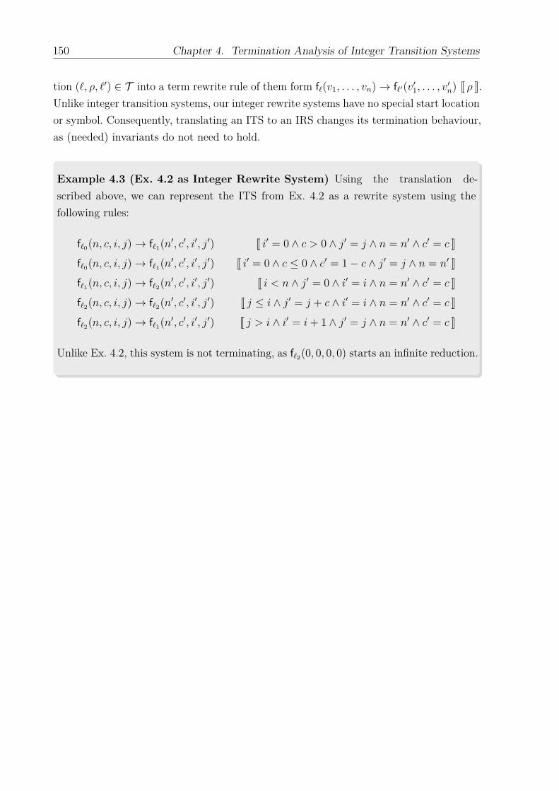
150 Chapter 4. Termination Analysis of Integer Transition Systems
tion (`, ρ, `′) ∈ T into a term rewrite rule of them form f`(v1, . . . , vn)→ f`′(v′1, . . . , v′n) J ρ K.Unlike integer transition systems, our integer rewrite systems have no special start locationor symbol. Consequently, translating an ITS to an IRS changes its termination behaviour,as (needed) invariants do not need to hold.
Example 4.3 (Ex. 4.2 as Integer Rewrite System) Using the translation de-scribed above, we can represent the ITS from Ex. 4.2 as a rewrite system using thefollowing rules:
f`0(n, c, i, j)→ f`1(n′, c′, i′, j′) J i′ = 0 ∧ c > 0 ∧ j′ = j ∧ n = n′ ∧ c′ = c K
f`0(n, c, i, j)→ f`1(n′, c′, i′, j′) J i′ = 0 ∧ c ≤ 0 ∧ c′ = 1− c ∧ j′ = j ∧ n = n′ K
f`1(n, c, i, j)→ f`2(n′, c′, i′, j′) J i < n ∧ j′ = 0 ∧ i′ = i ∧ n = n′ ∧ c′ = c K
f`2(n, c, i, j)→ f`2(n′, c′, i′, j′) J j ≤ i ∧ j′ = j + c ∧ i′ = i ∧ n = n′ ∧ c′ = c K
f`2(n, c, i, j)→ f`1(n′, c′, i′, j′) J j > i ∧ i′ = i+ 1 ∧ j′ = j ∧ n = n′ ∧ c′ = c K
Unlike Ex. 4.2, this system is not terminating, as f`2(0, 0, 0, 0) starts an infinite reduction.

4.2. Termination Proving by Safety Proving 151
4.2 Termination Proving by Safety ProvingAs discussed above, many recent termination proving techniques build on fully automaticsafety provers, i.e., tools that can prove certain “unsafe” program states to be unreachable.We will not discuss the details of safety proving, but only define the general propertyconsidered by them:
Definition 4.4 (Safety) Let P = (L,V , T ) be a Integer Transition System and err ∈ Lthe canonical error location. We call P safe if there is no run (`0,x0), . . . , (err ,xe) in P.
For the following, we fix P = (L,V , T ) as the considered program. In Sect. 4.2.1, wefirst present the reduction of termination analysis to a safety problem in detail, closelyfollowing the approach in [CSZ13]. We then present a new interpretation of this idea inSect. 4.2.2 in the form of cooperation graphs. In contrast to earlier work, these graphsallow to couple the power of standard safety provers with many standard techniques fromtermination analysis of declarative languages, e.g., the simplification-oriented methodsfrom Chapter 3. This results in a solution that greatly improves the performance andprecision of the overall approach.
4.2.1 Iterative Construction of Termination Arguments
We again construct lexicographic termination arguments. However, unlike our approachfollowing the DP Framework in Chapter 3, we will now explicitly construct such a lexi-cographic termination argument. For this, we combine linear rank functions as programmeasures, and require them to be decreasing over the course of a program run. We alsorequire these measures to be bounded from below. To delegate proving these propertiesfor a given rank function to a safety prover, we consider the dual problem and try to showthat in no program run, the measure increases or decreases below a certain bound. Forthis, we take snapshots of the program variables at certain points. Then, we can use thesafety prover to compare the value of the chosen measure at the time of the snapshot withits value at a later point. We can then check the necessary conditions of a terminationproof, i.e., show that the measure does not increase and that it is always greater than ourspeculated lower bound.
We do not need to allow such program state snapshots in every program evaluation step.It suffices to restrict this to the cutpoint set of a program [Flo67], where a cutpoint setdescribes those locations that are always used again and again in an infinite computation.More formally, a cutpoint set is a minimal set of vertices in the program graph that, ifremoved, leaves a program graph without cycles.
Definition 4.5 (Cutpoint Set) We call Cutpoints(P) ⊆ L a cutpoint set if (L \Cutpoints(P),V , {(`, ρ, `′) ∈ T | `, `′ 6∈ Cutpoints(P)}) is a program graph with-out cycles.

152 Chapter 4. Termination Analysis of Integer Transition Systems
Input: Program P = (L,V , T )Output: Transitions T ′ reaching err if not proven terminating1: T ′ = T2: for all p in Cutpoints(P) do3: pc := CutpointDuplicate(p)4: for all (p, ρ, `) in T do5: T ′ := (T \ {(p, ρ, `)}) ∪ {(pc, ρ, `)}6: end for7: T := T ∪ {(p, snapshot(p), pc), (p, nosnapshot(p), pc)}8: T := T ∪ {(p, spp > 0, err)}9: end for
10: return TAlgorithm 1: Instrument, preparing the termination as safety instrumentation.
In a first step, we present the changes needed to allow a safety prover to check atermination argument. To extend the input program to take snapshots of variable values,we create a copy vc of each variable v ∈ V . Then, for each cutpoint location p, we createa duplicate location pc. Between the two, we will allow to take a snapshot. For this, weadd one transition between p and pc in which we create no snapshot, and hence no valuesare changed. The second transition we create sets all variables vc to the current value ofv for all v ∈ V. Furthermore, we set a (boolean) flag spp = 1 to indicate that a snapshotwas taken. Then, we just “move” all transitions starting in p to start in its newly createdduplicate pc. Thus, our program now behaves as before, but additionally allows to createvariable snapshots at the beginning of a loop and check these after one iteration of thatloop.
The structure of our termination arguments allows us to only consider one loop iterationat a time. Hence, once we have taken a snapshot at the beginning of a loop, we just needto check that our chosen measure decreases in each loop iteration, but do not need toconsider the behaviour of several loop iterations together. Thus, we only allow to use thetransitions between p and pc if spp is not set. Finally, we add an error location err to ourprogram. Then, for each cutpoint p ∈ P , we add a transition from p to err that is enabledif our termination argument does not hold. Initially, we have no termination argument, sowe allow a transition to the error location whenever we have already taken a snapshot.
The algorithm Instrument in Fig. 1 performs this instrumentation. Here, theauxiliary method snapshot creates the transition label to copy all variables and setand check spp, and nosnapshot creates the transition label that does nothing butcheck spp.
Example 4.6 (Ex. 4.2 Instrumented) Applying Instrument to the exampleprogram P1 from Fig. 4.1(b) results in Fig. 4.2. Here, we used Cutpoints(P1) = {`2}.

4.2. Termination Proving by Safety Proving 153
`0
`1
`c2`2
err
τ0 : i := 0if(c > 0)
τ1 : i := 0if(c <= 0)c := 1− c
τ2 : if(i < n)j := 0
γ`2 : if(sp`2 ≤ 0)nc := ncc := cic := ijc := jsp`2 := 1
η`2 : if(sp`2 ≤ 0)
τ3 : if(j > i)i := i+ 1
τ4 : if(j ≤ i);j := j + c;
θ`2 : if(sp`2 > 0)if(¬false)
Figure 4.2: Instrumented version of Fig. 4.1
Proving termination of the original program is now possible by repeated safety checkingof the instrumented version. When safety checking fails, the safety prover provides a runending in the error location err that is a counterexample to our current terminationargument. Based on this counterexample, we then speculate a new termination argumentthat hopefully generalises to the whole program. The counterexamples returned by thesafety prover take the form of a lasso: A stem leading to some cutpoint p, where we take asnapshot of the program state, and then a cycle leading back to the cutpoint p, from whichwe then reach the error location. Intuitively, the meaning of the found counterexample isthat after the found stem, the cycle may be executed an infinite number of times; or atleast that our termination argument does not yet explain why this is not the case.
Example 4.7 (Lasso and Stem of a Counterexample) We again consider P1 fromFig. 4.1(b). Applying Instrument to P1 results in Fig. 4.2, where we usedCutpoints(P1) = {`2}. A safety prover now might return the counterexample
π1 = 〈τ0, τ2, γ`2 , τ4, θ`2〉
The stem of π1 is 〈τ0, τ2〉 and its cycle is 〈γ`2 , τ4〉. Thus, the cycle of the counterexampleπ1 corresponds to one iteration of the inner loop of the program P1.

154 Chapter 4. Termination Analysis of Integer Transition Systems
To gain as much information as possible from the concrete structure of the counterexam-ple, we use a simple symbolic integer domain [Min06] and abstract interpretation [CC77].For this, we restrict ourselves to program runs in which the stem of the counterexampleis executed first, and then the cycle is repeated an arbitrary number of times. We callan invariant that holds for all of these program runs a path invariant and use it to sup-port our rank function synthesis. This is based on the intuition that a counterexamplerepresents a “class” of similar program runs, and that a path invariant obtained from thecounterexample is likely to hold for program runs from that class.
Definition 4.8 (Lasso, Stem, Cycle, Path Invariant of a Counterexample)Let the run π = τ0 . . . τnθ be a counterexample to safety of a program graph obtainedfrom Instrument(P), where θ = (p, ρ, err). Then, there is some transition τi =(p, ρi,CutpointDuplicate(p)) and we call σ = τ0 . . . τi−1 the stem of π and φ =τi τi+1 . . . τn the cycle of π.We define the path invariant of φ as the integer invariants we can discover for V in
the program restricted to program runs of the form σφ∗ (i.e., where σ is followed by anarbitrary number of repetitions of φ). Then we define the cycle formula ϕ for π as theconjunction of the path invariant and the combined labels of all transitions of φ.
Example 4.9 (Path Invariants from Counterexamples) For the counterexampleπ1 from Ex. 4.7, we obtain the path invariant c > 0∧ i = 0∧ i < n∧ j ≥ 0. We combinethis with the representation of the cycle, yielding the cycle formula
ϕ1 = c > 0 ∧ i = 0 ∧ i < n ∧ j ≥ 0 ∧ j ≤ i ∧ j′ = j + c ∧ n′ = n ∧ c′ = c ∧ i = i′
Our goal is to find a rank function that proves the program runs represented by ourcounterexample to be terminating. To this end, we use the technique we described inSect. 3.4, restricted to a single program transition. For this transition, described by thecycle formula, we want a rank function f that strictly decreases in each iteration allowedby the transition label, so we require f(v1, . . . , vn) > f(v′1, . . . , v′n). We also want f to bebounded from below, and fix this bound to be 0 and hence just require f(v1, . . . , vn) ≥ 0.
Example 4.10 (Rank Functions From Counterexamples) For the cycle formulaϕ1 from Ex. 4.9, we can obtain the rank function f1(n, c, i, j) = i − j, as the followingtwo conditions indeed hold:
ϕ1 =⇒ f1(n, c, i, j) = i− j > i′ − j′ = f1(n′, c′, i′, j′)
ϕ1 =⇒ f1(n, c, i, j) = i− j ≥ 0

4.2. Termination Proving by Safety Proving 155
`0
`1
`c2`2
err
τ0 : i := 0if(c > 0)
τ1 : i := 0if(c <= 0)c := 1− c
τ2 : if(i < n)j := 0
γ`2 : if(sp`2 ≤ 0)nc := ncc := cic := ijc := jsp`2 := 1
η`2 : if(sp`2 ≤ 0)
τ3 : if(j > i)i := i+ 1
τ4 : if(j ≤ i);j := j + c;
θ′`2 : if(sp`2 > 0)if(¬(ic − jc > i− j ∧ ic − jc ≥ 0))
Figure 4.3: Strengthened version of Fig. 4.2
However, f ′1(n, c, i, j) = −j is also a valid rank function. It is obviously decreasing, andthe subformula j ≤ i ∧ i = 0 of ϕ1 ensures that f ′1 is always non-negative.
When a rank function for a counterexample was found, we have refined our terminationargument. Consequently, we also refine our program graph using this new rank function,and restrict the corresponding transition to the error location accordingly. We only wantto find new counterexamples that are not covered by the found termination argument, sowe change the label to require that either our rank function increased in a loop iteration(i.e., f(vc1, . . . , vcn) < f(v1, . . . , vn)) or that the rank function’s value is not bounded frombelow (i.e., f(vc1, . . . , vcn) < 0).
Example 4.11 (Strengthening Programs Graphs With Rank Functions) Weuse the rank function f from Ex. 4.10 to strengthen the transition θ`2 from `2 to errin Fig. 4.2. For this, we extend the label with ¬(ic − jc > i − j ∧ ic − jc ≥ 0)). Theresulting program graph, using θ′`2 instead of θ`2 is displayed in Fig. 4.3.
After we have changed our program graph to reflect the updated termination argument,the process can begin again. However, when we obtain a second counterexample, we need

156 Chapter 4. Termination Analysis of Integer Transition Systems
to combine the rank function found for this new counterexample with the rank functionsfound earlier. As we discussed above, we explicitly create lexicographic termination argu-ments [AG00, BMS05a, HM05, GTSF06, ADFG10, CGB+11]. For this, we use a sequenceof n ranking functions to map each program state to a vector of n values and use a lexico-graphic ordering on these vectors, i.e., we define (x1, x2, . . . , xn) > (y1, y2, . . . , yn) if andonly if x1 > y1 or n > 1, x1 = y1, and (x2, . . . , xn) > (y2, . . . , yn).To construct such a lexicographic argument, we consider all counterexamples found so
far for a certain cutpoint p, and their cycle formulas ϕ1, . . . , ϕm. We want to find a sequenceof m ranking functions f1, . . . , fm such that whenever one loop iteration represented bythe cycle formulas was performed, the overall measure of the program according to ourlexicographic combination decreases, or more formally, that the following holds:
m∨i=1
ϕi =⇒ (f1(v′1, . . . , v′n), . . . , fm(v′1, . . . , v′n)) > (f1(v1, . . . , vn), . . . , fm(v1, . . . , vn))
(4.1)
To describe and construct lexicographic termination arguments over program variablesv1, . . . , vn, we define two boolean auxiliary functions:
L>(f, ϕ)⇔ ϕ→ f(v′1, . . . , v′n) > f(v1, . . . , vn) ∧ f(v1, . . . , vn) ≥ 0
L≥(f, ϕ)⇔ ϕ→ f(v′1, . . . , v′n) ≥ f(v1, . . . , vn)
Using these, we can now describe our lexicographic ranking function synthesis problem aslooking for a permutation σ and rank functions f1, . . . , fm such that the following variationof (4.1) holds:
∨1≤i≤m
L>(fi, ϕσ(i)) ∧ ∧
1≤j<iL≥(fj, ϕσ(i))
(4.2)
In other words, σ is used to bring our counterexamples into some order fitting our rankingfunctions. For each counterexample we require that its relation is decreasing and boundedby one of the rank functions fi, while the value of all “prior” rank functions is not increasedby the relation of the considered counterexample.
Example 4.12 (Combining Several Counterexamples) We continue with thestrengthened program graph in Fig. 4.3 obtained in Ex. 4.11. The counterexample π1
from before is not valid in the changed program anymore, but a second counterexample,corresponding to the outer loop, can be found:
π2 = 〈τ0, τ2, η`2 , τ4, γ`2 , τ3, τ2, θ′`2〉

4.2. Termination Proving by Safety Proving 157
This counterexample corresponds to the first iteration of the outer loop of the program.We separate π2 into a stem σ2 = 〈τ0, τ2, η`2 , τ4〉 and a cycle φ2 = 〈γ`2 , τ3, τ2〉. The obtainedpath invariant is c > 0 ∧ i ≥ 0 ∧ i < n ∧ j ≥ 0 and thus, the following cycle formula isobtained:
ϕ2 = c > 0 ∧ i ≥ 0 ∧ i < n ∧ j ≥ 0 ∧ i′ = i+ 1 ∧ 1 > i′ ∧ i′ < n ∧ j′ = 0 ∧ c′ = c ∧ n′ = n
Note the atom 1 > i, which is an artifact of the check j > i on transition τ3. It stemsfrom our concrete counterexample, in which j is set to 1 at this point.
Our rank function synthesis for the two counterexamples π1, π2, results in 〈π2, π1〉 withrank functions 〈f2, f1〉, where f1 is as above, and f2(n, c, i, j) = n− i. Note that in thiscase, the value of f2 is invariant for the relation ϕ1, so (4.2) from above holds. We mightalso replace f2 by f ′2(n, c, i, j) = −i, which would satisfy (4.2) as well.
As before, we want to strengthen program graphs with the newly obtained terminationarguments. To this end, we need to encode a violation of the argument as a formula wecan use as label for a transition from cutpoints to the error location. For this, we nowdefine nodecrease, which takes as argument the cutpoint that is currently handledand a lexicographic termination argument to encode:
nodecrease(p, 〈f1, . . . , fm〉) = spp > 0
∧ ¬
∨1≤i≤m
fi(vc1, . . . , vcn) > fi(v1, . . . , vn)
∧ fi(vc1, . . . , vcn) ≥ 0
∧∧
1≤j<ifj(v,1 . . . , vcn) ≥ fj(v1, . . . vn)
Example 4.13 (Combining Several Counterexamples) We extend the programgraph of Fig. 4.3 with the lexicographic termination argument found in Ex. 4.12. Theresulting program graph, Fig. 4.4, replaces the transition θ′`2 by a new transition θ′′`2 ,labelled with the value of nodecrease(`2, 〈f2, f1〉).
On the new program graph, the safety proof succeeds, as standard safety provers areable to infer the (needed) invariant c > 0 from τ1. As the safety proof is equivalent to aproof of validity of the termination argument we constructed, we have proven terminationof our example.

158 Chapter 4. Termination Analysis of Integer Transition Systems
`0
`1
`c2`2
err
τ0 : i := 0if(c > 0)
τ1 : i := 0if(c <= 0)c := 1− c
τ2 : if(i < n)j := 0
γ`2 : if(sp`2 ≤ 0)nc := ncc := cic := ijc := jsp`2 := 1
η`2 : if(sp`2 ≤ 0)
τ3 : if(j > i)i := i+ 1
τ4 : if(j ≤ i);j := j + c;
θ′′`2 : if(sp`2 > 0)if(¬((nc − ic > n− i ∧ nc − ic ≥ 0)∨(ic − jc > i− j ∧ ic − jc ≥ 0∧ nc − ic ≥ n− i)))
Figure 4.4: Strengthened version of Fig. 4.3
The complete algorithm for this iterative termination analysis is displayed as algorithmRefinement in Fig. 2. There, we first use Instrument from Fig. 1 to transformour input program into a safety problem. Then, we initialise empty sequences Πp of coun-terexamples for each cutpoint p in our program, and start searching for counterexamples.Whenever a counterexample with stem stem leading to a cycle cycle on the cutpoint pis found, we extend Πp to store this counterexample. We then synthesise a lexicographicranking function as above and use it to strengthen the condition on the edge from p to theerror location. If no further counterexample is found, termination is proven. The algorithmRefinement matches the informal description of the approach given in [CSZ13].
The procedure Refinement is depending on a number of (non-obvious) choices. Forexample, when searching for a suitable rank function based on a set of counterexamples,we usually have several options. Not all of these eventually lead to a termination proof.
Example 4.14 (Wrong Choice of Rank Function) In Ex. 4.12, we used the rankfunction f2(n, c, i, j) = n− i. Instead, we could also use f ′2(n, c, i, j) = −i. The additionaln in f2 is not needed to show decrease of the rank function, but to ensure that it isbounded from below. In this case, this property follows from the conjunct i < n of thepath formula for our counterexample π2. The path formula also contains i′ = i+1∧i′ < 1,and so f ′2 is also a possible rank function. In general, rank functions using fewer variables

4.2. Termination Proving by Safety Proving 159
Input: Program POutput: “P Terminating” or “Unknown”1: T ′ = Instrument(P)2: for all p in Cutpoints(P) do3: Πp = 〈〉4: end for5: while ex. counterexample (stem, p, cycle) from `0 to err in T ′ do6: Πp = Πp · (stem, cycle)7: if ex. σ, f1, . . . , fn for Πp with (4.2) then8: T ′ := (T ′ \ {(p, τ, err}) ∪ {(p, nodecrease(p, 〈f1 . . . fn〉), err)}9: else10: return “Unknown”11: end if12: end while13: return “P Terminating”
Algorithm 2: Procedure Refinement
are preferable, as in our experience, they are more likely to generally hold. However, inour case, f ′2 would not allow to prove termination; instead another counterexample π3
would be returned:
π3 = 〈τ0, τ2, η`2 , τ4, η`2 , τ3, τ2, η`2 , τ4, η`2 , τ4, γ`2 , τ3, τ2, θ′`2〉
Here, another unrolling of the loop is considered. As i = 1 holds when a copy of thevariable values is made in γ`2 , f ′2(n, c, i, j) = −i is not bounded by 0 anymore, and hencethe transition to the error location is enabled. This would trigger the search for a newrank function, yielding either the (useful) f2 or f ′′2 (n, c, i, j) = 1− i. Choosing f ′′2 wouldlead to finding a new counterexample, corresponding to a second loop unrolling, andleading to the same process again.
Problems with choosing the right rank function as in Ex. 4.14 occur often in the presenceof nested loops where the inner and outer loops work on the same variables. In these cases,tools like Terminator often diverge.1 Choosing the right rank function often not onlydepends on the counterexamples considered so far, but also on the larger program context.In the next section, we will discuss a solution to this problem.
4.2.2 Cooperative Termination Proving
We now extend the older work described in Sect. 4.2.1. As discussed above, the success ofthe Terminator method depends on several uninformed choices in the termination
1In fact, Terminator is not able to prove termination of our bubble sort-like example in Fig. 4.1(a).

160 Chapter 4. Termination Analysis of Integer Transition Systems
argument synthesis. At the same time, definite results, i.e., termination arguments that werealready validated, do not simplify the safety proof. Other than the iterative simplification-based approach for Integer Term Rewriting presented in Chapter 3, the considered problemis not simplified by successful proof steps.In this section, we will present a cooperative termination analysis approach based on
safety proving. Here, the termination argument synthesis is strengthened by not onlyusing a few counterexamples, but also their program context. This reduces the numberof iterations until a correct termination argument is found, and sometimes is needed tomake the process converge. At the same time, the program is simplified when certaintermination arguments are found by removing transitions. This greatly simplifies the workof the underlying safety prover, improving performance of the overall analysis.
Example 4.15 (Removing Transitions Generally not Sound)
`0
`1
`2
τ0 : if(n > 0)i := 0τ2 : if(i < n)
i := i+ 1
τ1 : if(i ≥ n)τ3 : if(i = n);
i := i+ 1n := n+ 1
Figure 4.5: A simple program
The techniques from Chapter 3 cannotbe adapted directly to our termination-as-safety setting. To see why, consider the non-terminating example Fig. 4.5, in which twoloops occur after each other. We can easily finda rank function n− i that shows that τ2 is de-creasing and bounded from below. However,removing the transition is incorrect, as the re-maining program would be terminating. Theroot of this problem is that while some reach-able program states lead to non-termination(i.e., all those where n = i at location `2), they become unreachable when removing atransition.
In our method, program graphs serve two uses at the same time: They describe the setof reachable states, i.e., states which need to be considered for termination analysis (a setinteresting to the safety prover) and they record the state of our termination proof. Theseusages have diverging goals: To ensure soundness of the results of the safety checker, wemust ensure that the set of reachable states remains unchanged. For the termination proof,we want to simplify and reduce the problem as much as possible. A solution to this usageconflict is to duplicate the program information. In our cooperation graphs, we duplicateall program parts relevant for program termination (i.e., cycles in the program graph).
The original program is then used for safety analysis, while the duplicated parts can bemodified and simplified to record the state of termination analysis. Thus, the safety doesnot need to prove precise invariants for program parts that are already proven terminating.

4.2. Termination Proving by Safety Proving 161
`0
`1
`2
`t1
`t2 `c2
err
τ0 : i := 0if(c > 0)
τ1 : i := 0if(c <= 0)c := 1− c
τ2 : if(i < n)j := 0
τ3 : if(j > i)i := i+ 1
τ4 : if(j ≤ i);j := j + c;
ε`2 : skip
τ t2 : if(i < n)j := 0
γ`2 : if(sp`2 ≤ 0)nc := ncc := cic := ijc := jsp`2 := 1
η`2 : if(sp`2 ≤ 0)
τ t3 : if(j > i)i := i+ 1
τ t4 : if(j ≤ i);j := j + c;
θ`2 : if(sp`2 > 0)if(¬false)
Figure 4.6: Cooperation graph for Fig. 4.1
We connect the two subgraphs, allowing to jump from the safety to the terminationsubgraph (but not in the other direction).
Example 4.16 (Cooperation Graph) To illustrate cooperation graphs, we go backto the example from Fig. 4.1. The corresponding cooperation graph is displayed inFig. 4.6. There, nodes on the left and colored in gray are safety nodes, corresponding tothe initial program in Fig. 4.1. On the right, the (only) strongly connected componentof the program is copied, and its black termination nodes will be used to track theprogress of termination proof. Between the two, transitions at cutpoints allow to non-deterministically jump from the safety to the termination part of the graph. On the nodesof the termination subgraph, we used a procedure analogous to Instrument to allowto take program state snapshots and to check the validity of termination arguments.
In the resulting graph, reasoning about termination is performed on the terminationsubgraph by a procedure built around an efficient rank function synthesis, similar to themethods presented in Chapter 3. We can also adapt other techniques from the handling of

162 Chapter 4. Termination Analysis of Integer Transition Systems
int-TRSs, e.g., remove transitions and add eventual invariants. Reasoning about reachablestates and program invariants is performed on the combination of the two, where speculatedtermination arguments in the termination graph direct the search for invariants, and thesafety subgraph ensures that the set of reachable states does not change.
So the advantage of the duplication (i.e., the termination and safety subgraphs) is thatwe can easily restrict certain operations to either subgraph, but we maintain a connectionbetween them. Intuitively, the safety subgraph describes an over-approximation of all reach-able states, while the termination subgraph is an over-approximation of those states forwhich termination has not been proven yet. In our setting, iterative program simplificationsencode the progress of the termination proof search and are directly available to the safetyprover when searching for more counterexamples. The structure of the graph guides thesafety prover to unproven parts of the program, directly yielding relevant counterexamplesthat can be used by the rank function synthesis to produce better termination arguments.If these do not allow a program simplification, they still guide the generation of invariantsby the safety prover for nodes in the safety subgraph. These in turn then support reasoningabout the validity of termination arguments in the termination subgraph.So to prove termination, we use a mix of the techniques from Chapter 3 and of the
approach from Sect. 4.2.1. Again, we use counterexamples to the current termination argu-ment to drive the termination proof. However, when we find a counterexample, we do nottry to construct a termination argument from it alone. Instead, we consider all transitionsfrom the termination subgraph that are in the same strongly connected component (SCC)as the cycle of the found counterexample. We call this enclosing SCC the SCC context ofa cycle.For this SCC context, we try to find a rank function, using the same constraints as in
Sect. 3.24, i.e., we require that all transitions do not increase the program measure andsome are decreasing it. This allows us to avoid many heuristics needed to choose the “right”rank function, as additional information from the SCC is available. In Ex. 4.12, we neededto choose between “n− i” and “−i”. By considering the additional transitions in its SCCcontext, we can see that in general, −i is not bounded from below, and can hence makethe informed choice of “n− i”. When we can also prove that a transition always decreasesthe measure and is bounded from below, we can just remove it from the program graph.In any case, we can use the found rank function to strengthen the termination argument,as above.
Example 4.17 (Simplifying Cooperation Graphs) We prove termination ofFig. 4.1 using the cooperation graph in Fig. 4.6. We start searching for a counterexample,yielding the run
π′1 = 〈τ0, τ2, ε`2 , η`2 , τt4, γ`2 , τ
t3, τ
t2, θ′`2〉

4.2. Termination Proving by Safety Proving 163
Here, the stem σ′1 = 〈τ0, τ2〉 is drawn from the safety subgraph, and then the cycleφ′1 = 〈η`2 , τ t4, γ`2 , τ t3, τ t2〉 comes from the termination subgraph (here, we just ignore theconnecting transition ε`2). The SCC context of the cycle φ′1 is the entire terminationsubgraph, i.e., the nodes `t1, `t2, and `c2 and all their connecting transitions η`2 , γ`2 , τ t4, τ t3,and τ t2.We now try to find a rank function that not only takes the program variables, but
also the program location into account. For this, we generate point-wise rank functionsf`t1 , f`t2 , and f`c2 . In our example, we obtain
f 1`t2
(i, j, k, n) = n− i f 1`c2
(i, j, k, n) = n− i
f 1`t1
(i, j, k, n) = n− i+ 1
Using these, we the following inequalities hold for the transitions in the SCC (whererelevant parts of the transition formula are displayed as preconditions), showing thatall transitions do not increase the program measure, and τ t2 decreases it and is boundedfrom below:
γ`2 : n′ = n ∧ i′ = i ⇒ n− i ≥ n′ − i′
η`2 : n′ = n ∧ i′ = i ⇒ n− i ≥ n′ − i′
τ t2 : n′ = n ∧ i′ = i ⇒ n− i+ 1 > n′ − i′
τ t2 : i < n ⇒ n− i+ 1 ≥ 0
τ t3 : n′ = n ∧ i′ = i+ 1 ⇒ n− i ≥ n′ − i′ + 1
τ t4 : n′ = n ∧ i′ = i ⇒ n− i ≥ n′ − i′
Hence, we have proven that in every infinite computation, τ t2 can only occur finitely often.This allows to remove the edge τ t2 from the termination subgraph (without changingthe set of reachable states). As this disconnects a part of the SCC, we now perform asimplification step restricting the termination subgraph to nodes and transitions thatmay occur in a loop, removing `t1 and τ t3. The resulting, simplified cooperation graph isdisplayed in Fig. 4.7.
By examining the SCC context of a counterexample, and not only its cycle (e.g. τ t2 inthe SCC context considered in Ex. 4.17) we can see that the rank function n− i is a betterrank function than j−i because τ t2 modifies j. This solves the problem of finding a suitableheuristic for choosing rank functions in Sect. 4.2.1. Without τ t2, j appears as a constantand hence, j > i looks like a suitable candidate invariant supporting the well-foundednessof the measure j − i. At the same time, considering all transitions (and hence all runsthat are allowed by these transitions) allows to conclude that τ t2 cannot occur infinitely

164 Chapter 4. Termination Analysis of Integer Transition Systems
`0
`1
`2 `t2 `c2
err
τ0 : i := 0if(c > 0)
τ1 : i := 0if(c <= 0)c := 1− c
τ2 : if(i < n)j := 0
τ3 : if(j > i)i := i+ 1
τ4 : if(j ≤ i);j := j + c;
ε`2 : skip
γ`2 : if(sp`2 ≤ 0)nc := ncc := cic := ijc := jsp`2 := 1
η`2 : if(sp`2 ≤ 0)
τ t4 : if(j ≤ i);j := j + c;
θ′`2 : if(sp`2 > 0)if(¬(ic − jc > i− j
∧ ic − jc ≥ 0))
Figure 4.7: Simplified cooperation graph for Fig. 4.1
often in a program run. Based on this, we can remove it from the program graph, makingreasoning about it simpler.
In some cases, it is not possible to find such a suitable rank function. This may happenwhen the information on transitions alone does not suffice, but invariants only valid inthe specific program context are needed. An example of this is the simple example at thebeginning of this chapter, or the transition τ t4 in our example Fig. 4.7. In such cases, wecan fall back to the standard Terminator method, as discussed above in Sect. 4.2.1.
Example 4.18 (Strengthening Cooperation Graphs) We continue Ex. 4.17 andsearch for a counterexample in Fig. 4.7. Now, all possible cycles allowed in the terminationsubgraph use the transition τ t4, and we might find the counterexample
π′2 = 〈τ0, τ2, ε`2 , γ`2 , τt4, θ`2〉
Here, we cannot find a rank function for all transitions in the SCC context (as we didfor the first counterexample), as we are missing the crucial invariant c > 0. We fall backto the method from Sect. 4.2.1, in which we speculate a rank function for the programby searching one only for the counterexamples found so far. Again, this leads to the

4.2. Termination Proving by Safety Proving 165
Input: Program P = (L,V , T )Output: Cooperation graph C with start location SafetyLoc(`0)1: C := ∅2: for all (`, τ, `′) in T do3: C := C ∪ {(SafetyLoc(`), τ, SafetyLoc(`′))}4: end for5: for all (`, τ, `′) in SCC_Transitions(T ) do6: C := C ∪ {(TerminationLoc(`), τ,TerminationLoc(`′))}7: end for8: for all p in Cutpoints(P) do9: pt := TerminationLoc(p)10: pc := CutpointDuplicate(p)11: C := C ∪ {(SafetyLoc(p), skip, pt)}12: for all (pt, τ, `′) in C do13: C := (C \ {(pt, τ, `′)}) ∪ {(pc, τ, `′)}14: end for15: C := C ∪ {(pt, snapshot(p), pc), (pt, nosnapshot(p), pc)}16: C := C ∪ {(pt, spp > 0, err)}17: end for18: return C
Algorithm 3: Procedure InstrumentCoop, initialising a new cooperation graph.
rank function i− j, which we use to strengthen the label of transition θ′`2 . As before, nofurther counterexamples are found, and we have proven termination.
For a general approach, we first adapt Instrument from Alg. 1 to produce a coopera-tion graph. The resulting procedure InstrumentCoop is displayed in Alg. 3. We usetwo auxiliary mappings SafetyLoc and TerminationLoc that map locationsfrom the input program to fresh locations. In the first loop, we use SafetyLoc tocreate the safety subgraph of the cooperation graph by copying all transitions from theoriginal program. In the second step, we use the function SCC_Transitions toidentify all program transitions that are part of a non-trivial SCC, i.e., those transitionsthat may make the program non-terminating.2 We then create the termination subgraphby copying these transitions to new locations obtained from TerminationLoc. Weuse Safety(C) to refer to the safety subgraph of the graph induced by the transitions C,and Termination(C) to refer to the termination subgraph. The final step of Instru-mentCoop applies the snapshotting/termination argument checking instrumentationfrom Alg. 1 to the termination subgraph. In this step, we also connect cutpoints in thesafety subgraph to their corresponding counterparts in the termination subgraph.
2A non-trivial is an SCC with at least one edge.

166 Chapter 4. Termination Analysis of Integer Transition Systems
Example 4.19 (Constructing Cooperation Graphs) In Fig. 4.7, the locations `0,`1, `2 and their connecting transitions make up the safety subgraph and are created bythe loop in lines 2–4. The locations `t1 and `t2 and their outgoing transitions are createdby the loop in lines 5–6, and the additional transitions η`2 , γ`2 and θ`2 are introduced bythe final loop in Alg. 1.
To prove the correctness of our approach, we formalise the intuitive view of cooperationgraphs as a tool to split (infinite) program executions into a finite prefix (in the safetysubgraph) and an infinite suffix (in the termination subgraph). For this, we first considerthe structure of infinite program executions. As there are only finitely many programtransitions, an infinite execution has to eventually re-use only a limited set of recurrenttransitions, and these transitions are then used infinitely often in an infinite execution.
Definition 4.20 Let π = (`0,x0), (`1,x1), . . . be an infinite execution of P. Let ti be thetransition between states (`i,xi) and (`i+1,xi+1). Then, there is an index n and a setR ⊆ T of recurrent transitions such that for every m > n, there is a m′ > m withtm′ = tm ∈ R, i.e., every element of R appears infinitely often in π. W.l.o.g. we choose aminimal n such that `n is a cutpoint.
We then call σπ = (`1,x1), . . . , (`n,xn) the stem of π and φπ = (`n,xn), (`n+1,xn+1), . . .the cycle of the computation π (cf. the analogous definitions for counterexample runs inDef. 4.8). Note that φt does not need to be periodic. We define the set of recurrent transitionsof the program T as Tω = {t ∈ R | ∃ an execution π with recurrent transitions R}.
We now show that this natural split of infinite executions into a stem and a cycle ismirrored in the construction of our cooperation graphs:
Lemma 4.21 (Cooperation Graphs Sound) Let C = InstrumentCoop(P),π be an infinite execution of P, and n, σπ, and φπ as in Def. 4.20. Then, there arecorresponding configuration sequences σ′π and φ′π such that σ′π φ′π is an infinite executionin C, with σ′π in Safety(C) and φ′π in Termination(C).
Proof. Let π = (`0,x0), (`1,x1), . . .. As Safety(C) is just a copy of the original program,we can just define
σ′π = (SafetyLoc(`0),x0), . . . , (SafetyLoc(`n),xn)
Here, line 3 of the algorithm Instrument ensures that the corresponding transitionsexist.

4.2. Termination Proving by Safety Proving 167
By choice of n, `n is a cutpoint. Hence, our cooperation graph contains a transition(SafetyLoc(`n), skip,TerminationLoc(`n)). As all remaining transitions in theexecution after (`n,xn) get used an infinite number of times, they have to be part of anSCC, and hence, by line 6 of the algorithm, copies of them exist in Termination(C).Consequently, we can then construct φ′π by starting with (TerminationLoc(`n),xn)and then simulating the infinite suffix (`n,xn), . . . of the original execution π. For thissimulation, we can just use the copied transitions. Only at cutpoints, where lines 8–16 ofInstrument introduce additional transitions to take value snapshots, additional stepsneed to be introduced in π′t to accommodate the use of the (unrestricted) nosnapshottransition. �
Our complete termination proving RefinementCoop procedure is displayed asAlg. 4. First, an input program is turned into a cooperation graph. Then, in a first pre-processing loop, as many transitions as possible are removed by searching for a suitableranking function for a complete SCC. This essentially means that the techniques fromChapter 3 are applied to the termination subgraph. Then, the procedure follows anadaption of Refine from Alg. 2. If a counterexample to the current set of terminationarguments is found, we first try to find a rank function that allows the removal of moretransitions in the loop. If that is not possible, we fall back to the procedure from the originalrefinement procedure, trying to find a lexicographic rank function for all counterexamplesfound so far. This is then used to strengthen the transition to the error location.
In RefinementCoop, we use S-orienting rank functions, which are similar to thereduction pairs of Sect. 3.4. Such rank functions ensure that all transitions in S do notincrease the state measure, and that at least one decreases it and bounds it from below.3
Definition 4.22 (S-orienting Rank Functions) Let S be a set of transitions. We callf : L× (V → Z)→ Z an S-orienting rank function if and only if there is some non-emptysubset S> ⊆ S such that the following two conditions hold:
∧(`,A(xx′
)≥a,`′)∈S
∀x,x′.A(xx′
)≥ a→ f((`,x)) ≥ f((`′,x′))
∧(`,A(xx′
)≥a,`′)∈S>
∀x,x′.A(xx′
)≥ a→ (f((`,x)) > f((`′,x′)) ∧ f((`,x)) ≥ 0)
We set Decreasing(S, f) = S>.
Based on this, we can prove that our transition removal in the termination subgraphis sound. We show that if t appears in the set of infinitely recurring transitions of some
3So if we represent the transitions in S as rewrite rules RS as in Ex. 4.3, a S-orienting rank function canbe obtained by finding a reduction pair (�,�) forRS with (RS)�∪(RS)� = RS , i.e., corresponding tothe conditions of the reduction pair processor RPProc of Def. 3.18. In this way, all methods presentedin Chapter 3 can be applied to our termination subgraph.

168 Chapter 4. Termination Analysis of Integer Transition Systems
Input: Program P with start state `0, transitions TOutput: “Terminating” or “Unknown”1: C := InstrumentCoop(T )2: for all S in SCCs(Termination(C)) do3: while ∃ S-orienting rank function f do4: C := C \ Decreasing(S, f)5: S := S \ Decreasing(S, f)6: end while7: end for8: for all p in Cutpoints(Termination(C)) do9: Πp = 〈〉10: end for11: while ex. counterexample (stem, p, cycle) from SafetyLoc(`0) to err in C do12: S := SCC_Context(Termination(C), cycle)13: Πp = Πp · (stem, cycle)14: if ex. S-orienting rank function f then15: C := C \ Decreasing(S, f)16: else if ex. σ, f1, . . . , fn for Πp with (4.2) then17: C := (C \ {(p, τ, err}) ∪ {(p, nodecrease(p, 〈f1 . . . fn〉), err)}18: else19: return “Unknown”20: end if21: end while22: return “P Terminating”
Algorithm 4: Procedure RefinementCoop, oscillating between a safety proverand a rank function synthesis tool using a cooperation graph.
transition set S, there is no S-orienting rank function f with t ∈ Decreasing(S, f)that would allow removal of t.
Lemma 4.23 (Transition Removal Sound) Let S be a set of transitions and t ∈ Sω.Then, there is no S-orienting rank function f with t ∈ Decreasing(S, f).
Proof. We prove the lemma by contradiction. If t ∈ Sω, there is an infinite S-executionπ = (`1,x1), (`2,x2), . . . such that the transition t is used infinitely often, i.e., we have aninfinite series of indices ι1, ι2, . . . such that t is used between (`ιi ,xιi) and (`ιi+1,xιi+1).Then, when applying f to the states in ρ and considering the constraints from Def. 4.22,we get the following series of inequalities:
f((`ι1 ,xι1)) > f((`ι1+1,xι1+1)) ≥ . . . ≥ f((`ι2 ,xι2)) > f((`ι2+1,xι2+1)) ≥ . . .
Transitivity of the order > on the integers then implies:
f((`ι1 ,xι1)) > f((`ι2 ,xι2)) > . . .

4.2. Termination Proving by Safety Proving 169
Thus, the value of f((`j,xj)) is infinitely decreasing. But Def. 4.22 also enforces thatthe value of f is non-negative at each use of t. Hence, no infinite sequence in whicht ∈ Decreasing(S, f) is used again and again exists. �
Hence, if we find a S-orienting rank function for an SCC in the termination subgraph,we can safely remove all decreasing transitions, as they are not infinitely recurring andhence cannot cause non-termination. We can now finally prove correctness of our algorithmRefinementCoop.
Theorem 4.24 If RefinementCoop(P) returns “Terminating”, P is terminat-ing.
Proof. We combine the results of Lemmas 4.21 and 4.23. Assume that P has an infiniterun π, but RefinementCoop returns “Terminating”.
Let C = InstrumentCoop(P). By Lemma 4.21, there exists an execution σ′π φ′π inInstrumentCoop(P) corresponding to π. As in Def. 4.20,π has an infinite suffix usingonly a restricted set of infinitely recurrent transitions R ⊆ T . By Lemma 4.23, the counter-parts of R in Termination(C) can never be decreasing under a Termination(C)-orienting rank function. Thus, the simplification steps in lines 4 and 11 of Refinementdo not remove these transitions. Hence, as “Terminating” is only returned when nocounterexample is found anymore, the condition on the path to the error location errgenerated by nodecrease has to be always false.This implies that there is a sequence of rank functions f1, . . . , fm on some cutpoint p
such that
¬
∨1≤i≤m
fi(s) > fi(s′) ∧ fi(s) ≥ 0 ∧ ∧
1≤j<ifj(s) ≥ fj(s′)
is always false for program states s, s′ connected by one loop iteration over p. Hence, wehave that the following holds for all possible such states:
∨1≤i≤m
fi(s) > fi(s′) ∧ fi(s) ≥ 0 ∧ ∧
1≤j<ifj(s) ≥ fj(s′)
By an argument similar to Lemma 4.23, this implies infinite descent in the well-foundedlexicographic order of > on m-tuples over the well-founded domain for our rank functions,and hence is a contradiction to our initial assumption that π is infinite. �
In practice, it is desirable to remove as many transitions as possible in the pre-processingstep of RefinementCoop. The reason for this are the relative performances of

170 Chapter 4. Termination Analysis of Integer Transition Systems
standard safety provers and rank function tools. Spending more time on obtaining more(and better) rank functions has almost no measurable cost relative to calling a safetyprover on a large example program. On the other hand, most loops in real programs areof a relative simple structure, and a more complex termination proving strategy is onlyrequired for a few hard loops. Reflecting this, we strengthen the program information usingthe abstract interpretation framework [CC77] to infer and propagate integer invariants,adding these to the constraints on our transitions. Here, the choice of a suitable integerdomain is important for the performance of the overall approach. We use the octagondomain [Min06] with an aggressive abstraction strategy, which seems to scale well to largeproblems. Using this extension for our example cooperation graph from Fig. 4.6 allowsto extend all transitions following `1 by the conjunct c > 0. Then, all transitions of thetermination subgraph can be removed in the pre-processing step, and the safety proverinstantly returns safety because the error location err is not reachable.

4.3. Alternating Termination/Non-termination Proving 171
4.3 Alternating Termination/Non-termination Proving
Proving non-termination represents an interesting complement to the problem of provingtermination. Unlike termination proving, which can be supported by a safety prover onlyconsidering finite program traces, non-termination proving requires reasoning about infiniteprogram runs. Beyond the obvious importance of proving non-termination for programverification, it has been shown to be useful for termination proving itself when combinedappropriately [HLNR10].In the following, we describe an approach which alternates between termination and
non-termination proving, making use of the structure of our cooperation graphs. The keyidea is to refine an over-approximation of the transitions that may occur in an infinitecomputation using termination proving, and to refine an over-approximation of the set ofreachable states by non-termination proving. So when a termination proof step using ourtechniques from Sect. 4.2 succeeds, we can reduce the number of transitions to considerin the remaining proof. When it fails, we obtain a counterexample that we can use torefine the termination argument, or to construct a possible non-termination argument. Anon-termination argument takes the form of a set of states that start an infinite evaluation,and we validate it by asking a safety prover to check reachability of the non-terminatingset of states. Disproving this requires finding a suitable program invariant. So if the non-termination proof fails, we can use this program invariant to strengthen our program, andbegin another termination proving attempt based on the new information.In the following, we first discuss a number of techniques to construct non-termination
arguments in Sect. 4.3.1. Then, in Sect. 4.3.2, we combine this into an alternatingtermination/non-termination proving procedure.
4.3.1 Synthesising Recurrent Sets
A proof of non-termination requires to show that the input program has an infinite run.For this, we adapt the notion of recurrent sets of states from [GHM+08]. A recurrent setdescribes program configurations that always start an infinite run. Formally, we requirethat for each state s in a recurrent set, there is an evaluation starting in s that eventuallyleads to a state s′ in the recurrent set. Furthermore, at least one of the states in therecurrent set needs to be reachable from the program start. In contrast to the originaldefinition of [GHM+08], we extend this notion to several program locations, and assignone set of recurrent states R` to each program location `. Following [HLNR10], we alsodefine the weaker notion of partial recurrent sets, which do not need to be reachable fromthe program start.

172 Chapter 4. Termination Analysis of Integer Transition Systems
if(x ≥ 0 ∧ k ≥ 0) thenwhile x 6= 0 do
x := x + k;done
fi
(a) Imperative program
`0
`1
τ0 : if(x ≥ 0 ∧ k ≥ 0)
τ1 : if(x 6= 0);x := x+ k;
(b) Program graph
Figure 4.8: A simple non-terminating program
Theorem 4.25 (Recurrent Sets) Let P = (L,V , T ) be a program. P has a partialrecurrent set if and only if there is a set R` for each ` ∈ L such that the followingconditions hold:
∃` ∈ L.R` 6= ∅ (4.3)
∀` ∈ L.∀(`,x) ∈ R`.∃(`′,x′) ∈ R`′ .(`,x)→ (`′,x′) (4.4)
Then, R = ⋃`∈LR` is a partial recurrent set. If any state from R is reachable from
the start location, i.e., if (`0,x0) →∗ (`,x) ∈ R holds, we call R a recurrent set. P isnon-terminating if and only if it has a recurrent set.
Proof. “⇒”: Let (`0,x0) → (`1,x1) → . . . be an infinite run. Then, we can construct arecurrent set by defining R` = {(`i,xi) | `i = `}.“⇐”: We construct an infinite run step-wise. We start with an arbitrary run of the
form (`0,x0)→n (`,x) ∈ R for some n ∈ N0. Then, each such run can be extended with(`,x)→ (`′,x′) by (4.4), i.e., we then have a longer run (`0,x0)→n+1 (`′,x′) ∈ R. �
Example 4.26 ((Partial) Recurrent Sets) We consider the program P in Fig. 4.8.Here, R`0 = ∅ and R`1 = {(`1, v) | v(x) < 0 ∧ v(k) ≤ 0} define a partial recurrent setfor P . However, R is not reachable, and a safety prover would need to infer the invariantx ≥ 0 ∧ k ≥ 0 for the loop to prove this.The sets R`0 = ∅ and R`1 = {(`1, v) | v(x) > 0 ∧ v(k) ≥ 0} make up another partial
recurrent set, which is indeed reachable from the start state with inputs x = 1, k = 1.
Obviously, as recurrent sets are a complete criterion for non-termination, we generallycannot decide if a recurrent set exists for a given program P . However, we will now present

4.3. Alternating Termination/Non-termination Proving 173
a number of incomplete procedures that can generate suitable partial recurrent sets formany examples. Obviously, the techniques from Sect. 2.5 and Sect. 3.7 can be adapted tofind recurrent sets. Here, looping non-termination corresponds to one-element recurrentsets (as the same program state is reached over and over again). Our technique for findingcases of non-looping non-termination results in recurrent sets described by conjunctionsof conditions occurring on program paths. While these techniques lead to very simpleconstraint systems, they often fail to find recurrent sets for interesting examples.
In the following, we extend a method from [GHM+08], which is using a template-basedtechnique to find recurrent sets. For this, a recurrent set is symbolically represented usinga system of linear inequalities templates, and then the conditions of Thm. 4.25 are encodedas a (non-linear) integer arithmetic problem that can be solved by a constraint solver. Amodel for the resulting formula that instantiates the template. In contrast to the originalapproach, our extension is able to handle non-deterministic programs and several programpoints.
To adapt this to several program points, we represent each recurrent set R` by a systemof (symbolic) linear inequalities, and let R` be the solutions to these inequalities. Usingnotation from linear algebra and ordering our program variables V as {v1, . . . , vn}, wedenote these template systems as T` · (v1, . . . , vn)t ≤ t`. Based on these templates, weexpress the conditions of Thm. 4.25 using only integer arithmetic. For this, membership of astate (`,v) in a recurrent set (i.e., (4.3)) is encoded as T` ·v ≤ t`. To express (`,v)→ (`′,v′)from (4.4), i.e., that a transition from T evaluates (`,v) to (`′,v′), we use the formula∨
(`,Ax≤a,`′)∈T A · (v v′)t ≤ a.So if P = (L,V , T ) is our program and V a set of fresh (integer-valued) variables
V , we create existentially quantified template matrices and vectors T` ∈ V k×n, t` ∈ V k,where n = |V| is the number of program variables and k ∈ N>1 determines the numberof inequalities used for each recurrent set.4 Then, we can express the constraints (4.4) ofThm. 4.25 as follows:
∀v.∧`∈L
T` · v ≤ t` =⇒∨
(`,Ax≤a,`′)∈T∃v′.A · (v v′)t ≤ a ∧ T`′ · v′ ≤ t`′
(4.5)
However, this constraint system is rather unsuitable for our purposes – its quantifieralternation and the used non-linear integer arithmetic is beyond the reach of modernconstraint solving tools. So in the following, we will discuss a number of modificationsto this system. Of course, we cannot avoid the non-linearity of the constraints, whichstems from our use of templates for recurrent sets. On the other hand, the alternation of
4The choice of k is a trade-off between power and performance of the method. Small values of k greatlyreduce the size of the generated formula, and thus allow the constraint solving back-end to find moresolutions. On the other hand, certain recurrent sets can only be described by a larger number ofconstraints. In practice, we use values of k between 1 and 4 and only test larger values when solvingthe system for a smaller value failed.

174 Chapter 4. Termination Analysis of Integer Transition Systems
quantifiers is not needed in all cases.The method originally proposed in [GHM+08] is restricted to deterministic programs,
and uses this to significantly simplify the constructed constraint system. In (4.5), we donot compute an explicit value for v′ (i.e., the values of all variables after using a transition(`, A · (v v′)t ≤ a, `′)), but allow a choice of values that satisfies our transitions constraint.This is needed in cases a program uses non-deterministic output, i.e., contains a statementlike x = rand(). However, if a program does not use random input, we can always separatethe label A · (v v′)t ≤ a of a transition τ into a set of guard constraints Gτ · v ≤ gτ onthe pre-variables of a transition and an update v′ = Uτv + uτ that maps the values ofpre-variables to the values of the post-variables. In that case, we can replace occurrencesof v′ in (4.5) after using transition τ by the term Uτv + uτ , and obtain the followingconstraint:
∀v.∧`∈L
T` · v ≤ t` =⇒∨
τ=(`,Ax≤a,`′)∈TGτ · v ≤ gτ ∧ T`′ · Uτ · v ≤ t`′ − T`′ · uτ
(4.6)
Then, we can use the well-known Farkas’ Lemma from linear algebra to eliminate theuniversally quantified v from (4.6):
Theorem 4.27 (Farkas’ Lemma [Far02]) Let A · x ≤ a be a satisfiable system oflinear inequalities over the reals. Then, ∀xA · x ≤ a =⇒ c · x ≤ d holds if and only ifthere exists a non-negative vector λ such that λ · A = c and λ · a ≤ d.
While Farkas’ Lemma is not complete over integer-valued variables, it is still sound,and thus applicable to our case. To apply it, we have to transform the constraints of (4.6)into a disjunction of implications. The resulting system is finally suitable for automatichandling by current constraint solvers.
Definition 4.28 (Synthesising Recurrent Sets for Deterministic Programs)Let P = (L,V , T ) be a deterministic program, k ∈ N≥1, and V a set of fresh (integer-valued)variables V . Furthermore, let T` ∈ V k×n, t` ∈ V k be template matrices, where n = |V| isthe number of program variables. Then, we can express the constraints of Thm. 4.25 asfollows, where Λ` ≥ 0 means that all entries of the matrix Λ` are non-negative:
∧`∈L
∨τ=(`,ρ,`′)∈T
∃Λ` ≥ 0. Λ` · T` = Gτ
T` · Uτ
∧ Λ` · t` ≤
gτ
t`′ − T`′ · uτ
(4.7)
Example 4.29 (Synthesising Recurrent Sets for Deterministic Programs)We return to the example program P in Fig. 4.8. To represent τ1 using matrices, we

4.3. Alternating Termination/Non-termination Proving 175
first split the implicit disjunction of x 6= 0, obtaining τ1,< = x < 0 ∧ x′ = x + k andτ1,> = x > 0 ∧ x′ = x + k. We can represent these two deterministic transitions usingthe following matrices and vectors:
Gτ1,< =(
1 0)
gτ1,< =(−1)
Uτ1,< =1 1
0 1
uτ1,< =0
0
Gτ1,> =
(−1 0
)gτ1,> =
(1)
Uτ1,> =1 1
0 1
uτ1,> =0
0
Then, (4.7) is satisfied for some (uninteresting) values of Λ and the following instantiationof our (two-dimensional) template:
T`1 =1 0
0 1
t`1 =−1
0
Indeed, T`1 · (x k)t ≤ t`1 is equivalent to the two inequalities x ≤ −1 and k ≤ 0, matchingthe first recurrent set for P we found in Ex. 4.26.
While this approach applies to many programs that are of interest in nonterminationanalysis, non-deterministic programs do occur and need to be handled. A number ofsolutions to this problem exist. One, closed recurrent sets [CCF+13], strengthens therestrictions of recurrent set to require that every instantiation of non-deterministicallychosen values has to lead back to the recurrent set. To model this, we do not use an affineupdate function Uv + u, but a system of inequalities. So our representation is similar tothe original transition label Ax ≤ x, but now separates constraints on the pre-variablesfrom constraints on the post-variables.
For this, we model the relation between pre- and post-variables using two matrices U , U ′
and a vector u. Then, v,v′ just needs to satisfy the inequalities(U U ′
)· (v v′)t ≤ u.
Based on this, we can adapt (4.6) to the non-deterministic case. For this, we require thatthe recurrent set at the source location entails the guard of at least one transition and thatevery allowed instantiation of the (possibly non-deterministically chosen) post-variablesis part of the recurrent set at the target location:
∀vv′.∧`∈L
∨τ=(`,Ax≤a,`′)∈T
(T` · v ≤ t` =⇒ Gτ · v ≤ gτ)
∧(T` · v ≤ t` ∧
(U U ′
)·
vv′
≤ u =⇒ T`′ · v′ ≤ t`′)(4.8)

176 Chapter 4. Termination Analysis of Integer Transition Systems
This constraint is stricter than necessary. Whereas here, we require that all evaluationslead back to the recurrent set, it would suffice to require that at least one does. However,this weaker constraint is not easily formalised as a constraint system, whereas we canagain modify (4.8) this to make use of Farkas’ Lemma, to avoid quantifier alternation.
Definition 4.30 (Synthesising Recurrent Sets for Non-deterministic Programs)Let P = (L,V , T ) be a program, k ∈ N≥1, and V a set of fresh (integer-valued) variablesV . Furthermore, let T` ∈ V k×n, t` ∈ V k be template matrices, where n = |V| is the numberof program variables. Then, we can express the constraints of Thm. 4.25 as follows:
∧`∈L
∨τ=(`,ρ,`′)∈T
∃Λ` ≥ 0,Λ′` ≥ 0,Λ′′` ≥ 0.Λ` 0
Λ′` Λ′′`
T` 0Uτ U ′τ
=Gτ 0
0 T`′
(4.9)
∧
Λ` 0Λ′` Λ′′`
t`uτ
≤gτt`′
In [CCF+13], a more refined procedure for obtaining recurrent sets based on precondition
inference via safety proving is presented. We will not discuss the details here, but want tonote that numerous approaches to solve the synthesis problem for recurrent sets exist.
4.3.2 Alternation
After identifying a (partial) recurrent set R for a given program P , we need to check if itis reachable from the program start. For this, we again use a standard safety prover, as wedo for our termination proving procedure in Sect. 4.2. In the following, we use formulasωR` to define the program configurations in a partial recurrent set at location ` and meanthat every configuration (`,v) where v satisfies ωR` is element of the recurrent set. Wecan easily obtain these formulas as a conjunction of the inequalities in our instantiationof the templates T` from above. To check that a recurrent set is reachable, we thus addedges (`, ωR` , err) to our program. If the safety prover then returns a counterexampleusing this edge, we have a proof that at least one program run exists that leads to aconfiguration which is part of the chosen recurrent set. Hence, in that case, the programis non-terminating.
Example 4.31 (Reachability of Recurrent Sets) We again return to our examplefrom before, now displayed as Fig. 4.9(a) with transitions labelled by the used formulas(where all lines are combined by conjunction). In Ex. 4.26, we found the partial recurrentset ω`1 = x < 0 ∧ k ≤ 0 for `1. In Fig. 4.9(b), we added an additional transition to the

4.3. Alternating Termination/Non-termination Proving 177
`0
`1
τ1 : x ≥ 0k ≥ 0x′ = xk′ = k
τ2 : x 6= 0x′ = x+ kk′ = k
`0’
`1’ err
τ1 : x ≥ 0k ≥ 0x′ = xk′ = k
τ2 : x 6= 0x′ = x+ kk′ = k
τ3 : x < 0 ∧ k ≤ 0
(a) (b)
Figure 4.9: First iteration of a non-termination proof
error location err that is only enabled if ω`1 holds. Then, a safety checker is able to provethis modified program safe, as the invariant x ≥ 0 ∧ k ≥ 0 holds.
If the chosen recurrent set is proven unreachable, a program invariant was producedin the safety proof. We want to make use of this invariant in further proof steps, andthus extract it from the safety proof and add it to our program. For this, we just addthe obtained invariant for a location ` as a new conjunct to the label of all transitionsstarting in `. Thus, we used the information obtained from refuting a non-terminationproof to strengthen the program, making restrictions on the invariants of our programmore explicit. Based on this strengthened program, we restart the recurrent set synthesis.As we added invariants refuting the reachability of prior recurrent sets, this now leads toa new partial recurrent set and the process can restart.
Example 4.32 (Reachability of Recurrent Sets and Invariants)We continue Ex. 4.31. From the safety proof of Fig. 4.9(b), we extract the invariantx ≥ 0 ∧ k ≥ 0. We then modify the program Fig. 4.9(a) to obtain Fig. 4.10(a). Here, weadded the invariant at location `2 to all transitions going out of `2.In the next step, we search for another recurrent set and use the second set from
Ex. 4.26, specified by ω′`1 = x > 0 ∧ k ≥ 0. We again construct a modified version of theprogram to check reachability, shown in Fig. 4.10(b). The safety prover now returns acounterexample 〈τ1, τ3〉, proving that the partial recurrent set is indeed reachable. Hence,we have proven non-termination.

178 Chapter 4. Termination Analysis of Integer Transition Systems
`0
`1
τ1 : x ≥ 0k ≥ 0x′ = xk′ = k
τ2 : x ≥ 0 ∧ k ≥ 0x 6= 0x′ = x+ kk′ = k
`0’
`1’ err
τ1 : x ≥ 0k ≥ 0x′ = xk′ = k
τ2 : x ≥ 0 ∧ k ≥ 0x 6= 0x′ = x+ kk′ = k
τ3 : x > 0 ∧ k ≥ 0
(a) (b)
Figure 4.10: Second iteration of non-termination proof of Fig. 4.9
Supporting Termination Proving The iterative strengthening of an input program byrelevant invariants is not only useful to direct a non-termination proof, but can alsostrengthen the termination proving process. The invariants obtained by refuting thereachability of non-terminating regions are intuitively related to the termination behaviour.
Example 4.33 (Termination by Non-termination Proving) We consider the ter-minating example program in Fig. 4.11(a). In this variation of Fig. 4.9(a), the crucialinvariant for a termination argument is k < 0. We again search for a partial recurrentset, obtaining ω`1 = x > 0 ∧ k ≥ 0. Using a safety prover to check reachability of statesdescribed by ω`1 refutes this as a non-termination argument, but yields the invariantk < 0. Adding this to the program yields Fig. 4.11(b), where we can trivially find therank function x, which is decreasing in each application of τ ′2.
In general, it is desirable to integrate termination and non-termination proving tech-niques in one approach. We adopt the idea of alternating provers of both kinds from[HLNR10]. However, we base our combined proving technique on cooperation graphs.Thus, a partial termination proof simplifies the program by removing transitions thatcannot contribute to an infinite computation. Based on the simplified termination sub-graph, we then synthesise partial recurrent sets. If such a set is reachable, we have provennon-termination. Otherwise, we strengthen the program transition using the invariantsobtained to refute the non-termination argument.Our procedure Alternation in Alg. 5 implements this idea. It is based on our
termination proving procedure RefinementCoop from Alg. 4, and extends it toincorporate non-termination proving. As before, we first build a cooperation graph and

4.3. Alternating Termination/Non-termination Proving 179
`0
`1
τ1 : k < 0x′ = xk′ = k
τ2 : x > 0x′ = x+ kk′ = k
`0
`1
τ1 : k < 0x′ = xk′ = k
τ ′2 : k < 0x > 0x′ = x+ kk′ = k
(a) (b)
Figure 4.11: Program before and after first iteration of a non-termination proof
then simplify it as far as possible. We then loop over the program to obtain counterexamplesto the termination argument constructed so far. For each counterexample, we first tryto further simplify our input program, i.e., find a termination argument that definitelyproves that a transition is only usable a finite number of times. If that is not possible,we try to synthesise a partial recurrent set for the SCC containing the counterexample.If we find one, we continue to check its reachability. If this succeeds, we haven provennon-termination. Otherwise, we use the obtained invariants to strengthen the program.This may allow further simplifications in the next iteration, or another partial recurrentset. If synthesising a partial recurrent set fails, we fall back to the original Terminatormethod and speculate a possible termination argument.Soundness of the procedure is a direct consequence of the soundness of the individual
components, and so we will not give an explicit proof here. It is important to note thatthe presented procedure is highly modularised: subprocedures such as the chosen tool tofind rank functions, prove safety, or find partial recurrent sets do not have to be modifiedfor their combination. Thus, independent further improvements to any of these techniquesare directly available to this alternating procedure.

180 Chapter 4. Termination Analysis of Integer Transition Systems
Input: Program P with start state `0, transitions TOutput: “Terminating”, “Non-terminating”, or “Unknown”1: C := InstrumentCoop(T )2: for all S in SCCs(Termination(C)) do3: while ∃ S-orienting rank function f do4: C := C \ Decreasing(S, f)5: S := S \ Decreasing(S, f)6: end while7: end for8: for all p in Cutpoints(Termination(C)) do9: Πp = 〈〉10: end for11: while ex. counterexample (stem, p, cycle) from SafetyLoc(`0) to err in C do12: S := SCC_Context(Termination(C), cycle)13: Πp = Πp · (stem, cycle)14: if ex. S-orienting rank function f then15: C := C \ Decreasing(S, f)16: else if ex. partial recurrent set R for S then17: if R reachable from `0 then18: return “Non-terminating”19: else20: strengthen C with refutation of reachability of R21: end if22: else if ex. σ, f1, . . . , fn for Πp with (4.2) then23: C := (C \ {(p, τ, err}) ∪ {(p, nodecrease(p, 〈f1 . . . fn〉), err)}24: else25: return “Unknown”26: end if27: end while28: return “P Terminating”
Algorithm 5: Procedure Alternation, oscillating between a termination and non-termination prover using a cooperation graph.

4.4. Evaluation 181
4.4 EvaluationWe implemented the described techniques in the tool T2. At this time, the implementationof the procedure Alternation (or, more precisely, the synthesis of recurrent setsrequired by it) is not stable enough for rigorous benchmarking. We will first discuss theevaluation of our cooperative refinement procedure, and then present some preliminaryresults for our alternation procedure.
4.4.1 Cooperative Termination Proving
To test the procedure RefinementCoop, we compared a number of configurationsof T2 and other termination provers handling integer programs:
• T2 [CSZ13], which implements the procedure Refinement from Alg. 2.
• Terminator [CPR06], which implements a technique similar to procedure toRefinement, but uses transition invariants [PR04b] to combine single rankfunctions (instead of a lexicographic combination). This is not the original imple-mentation evaluated in [CPR06], but its updated reimplementation in T2, usingthe exact same techniques.
• Cooperating-T2, which implements RefinementCoop from Alg. 4.
• ARMC [PR07], which also implements a Terminator-like procedure.
• AProVE using the techniques from Chapter 3. The techniques for handlingterms are obviously not needed here, and instead of considering a program with adesignated start, it just assumes that the evaluation could start anywhere. Thus, itsnon-termination techniques are activated (and often lead to aborting a terminationproof), but cannot yield “Non-terminating” as result.
• AProVE+Interp, which generates as many invariants as possible using theOctagon abstract domain [Min06] by calling the abstract interpretation tool In-terproc [JM09] before running AProVE. This is meant to mitigate thatAProVE ignores the start location and hence cannot make use of the initialisa-tion of certain variables.
• MCNP, an implementation of a method to prove termination using monotonicityconstraints [CGB+11], an efficient generalisation of the size-change principle [LJB01].The abstraction from integer programs to monotonicity constraints is implementedin AProVE.
• KITTeL [FKS11], another termination prover based on termination proving tech-niques from rewriting systems, similar to the techniques presented in Chapter 3.

182 Chapter 4. Termination Analysis of Integer Transition Systems
0.5 1 5 10 30 60120 300NR0.51
510
3060120300NR
T2 (s)
Co
ope
rat
ing
-T2(s)
0.5 1 5 10 30 60120 300NR0.51
510
3060120300NR
T2 (s)
Co
ope
rat
ing
-T2(s)
(a) (b)Figure 4.12: Evaluation results of Cooperating-T2 vs. Standard T2, in log scale.
Plot (a) represents the results of the two tools on terminating benchmarks, (b)represents non-terminating benchmarks. Timeout=300s. NR=“No Result”.The NR cases are due to failure of the underlying safety prover to find aninductive invariant.
During our evaluation we ran tools on a set of 449 termination proving benchmarksdrawn from a variety of applications that were also used in prior tool evaluations (e.g.,Windows device drivers, the Apache web server, the PostgreSQL server, integerapproximations of numerical programs from a book on numerical recipes [PTVF89], integerapproximations of benchmarks from LLBMC [MFS12] and other tool evaluations). Ofthese, 260 are known to be terminating and 181 are known to be non-terminating. For eightexamples, no result is known. These include the Collatz conjecture, and the remaining arevery large and hence have not been analysed manually. Our benchmarks and results canbe found at
http://verify.rwth-aachen.de/brockschmidt/Cooperating-T2/
Experiments for Terminator, T2, and Cooperating-T2 were performed on aquadcore 2.26GHz E5520 system with 4GB of RAM and running Windows 7. All otherexperiments were performed on a quadcore 3.07GHz Core i7 system with 4GB of RAMand running Debian Linux 6. We ran all tools with a timeout of 300 seconds. When a toolreturned early without a definite result or crashed, we display this in the plots using thespecial “NR” (no result) value.The results of our test runs are displayed in Fig. 4.12, Fig. 4.13, and the overview
table Tab. 4.1. Fig. 4.12 contains two plots which chart the difference between our newprocedure and T2’s previous procedure, in log scale. Plot (a) represents the results whenapplied to programs that terminate. Plot (b) contains the results from non-terminatingbenchmarks. Here both configurations of T2 use an approach similar to the approach used

4.4. Evaluation 183
0.5 1 5 10 30 60120 300NR0.51
510
3060120300NR
Terminator (s)
Co
ope
rat
ing
-T2(s)
0.5 1 5 10 30 60120 300NR0.51
510
3060120300NR
ARMC (s)
Co
ope
rat
ing
-T2(s)
0.5 1 5 10 30 60120 300NR0.51
510
3060120300NR
KITTeL (s)
Co
ope
rat
ing
-T2(s)
0.5 1 5 10 30 60120 300NR0.51
510
3060120300NR
MCNP (s)
Co
ope
rat
ing
-T2(s)
0.5 1 5 10 30 60120 300NR0.51
510
3060120300NR
AProVE (s)
Co
ope
rat
ing
-T2(s)
0.5 1 5 10 30 60120 300NR0.51
510
3060120300NR
AProVE-Interp (s)
Co
ope
rat
ing
-T2(s)
Figure 4.13: Evaluation results of Cooperating-T2 vs. other termination provingtools (see Fig. 4.12 for comparison to T2). Scatter plots are in log scale.Timeout=300s. NR=“No Result”, indicating failure of the tool.

184 Chapter 4. Termination Analysis of Integer Transition Systems
Term (#) Nonterm (#) Fail (#) avg. Term avg. Run.Cooperating-T2 245 174 30 3.42 13.77AProVE 197 0 252 2.21 47.23KITTeL 196 0 253 4.65 129.30T2 189 180 80 5.15 47.61AProVE+Interp 185 0 264 1.53 81.30Terminator 177 181 91 4.99 52.60MCNP 156 0 293 17.50 82.81ARMC 138 0 311 16.16 68.61
Table 4.1: Evaluation results of Cooperating-T2 and competing tools
in TnT [GHM+08] when finding a counterexample for which no rank function can befound (i.e., just before returning “Unknown”). We could not evaluate the non-terminationproving techniques in T2 against TnT, as we could not obtain the tool.Our method RefinementCoop from Alg. 4 has a fixed overhead, making non-
terminating proofs for examples where the first counterexample already suffices to find anon-termination argument slower. Additionally, our method exposes a performance/non-termination bug in Z3 in a few cases, leading to some additional timeouts. In non-terminating examples with many other terminating loops, our program simplificationsspeed up the search for a non-termination proof. Fig. 4.13 compares our procedure tothe other termination proving tools (to accommodate that not all tools support non-termination proofs, we only consider those examples that are not known to be non-terminating here). In Tab. 4.1 the first column indicates the number of successful ter-mination proofs, the second the number of successful non-termination proofs, and thethird the number of aborted/timed-out proof attempts. In the last two columns, the av-erage runtime (in seconds) of the tools is documented, where “avg. Term.” is the averagerestricted to successful termination proof attempts and “avg. Run.” is the average for allexamples. The improvement for terminating benchmarks is dramatic: Cooperating-T2 times out or fails far less often than competing tools. On non-terminating benchmarks,the difference is small.Overall, the performance gains of our approach over previous techniques are dramatic.
Our method does not just speed up termination proving, it also considerably improves caseswhere previous tools time out or fail. Our experimental results also show how importantsupporting invariants are, e.g., in Cooperating-T2 vs. AProVE we see thatmany results cannot be obtained without supporting invariants, as both tools essentiallyuse the same rank function synthesis algorithms. Further experiments have shown that avariation of Cooperating-T2 that does not delete transitions performs significantlyworse, failing on about 30 examples that Cooperating-T2 can handle. Furthermore,the result of AProVE+Interp indicates that an eager search for invariants in a

4.4. Evaluation 185
preprocessing step is not a suitable solution to this problem, as this leads to more timeouts.In-depth analysis shows that these are not only due to timeouts in the preprocessing toolInterproc, but that the wealth of generated invariants also slows down the latertermination proof.
4.4.2 Alternating Termination and Non-termination Proving
While a basic implementation of Alternation from Alg. 5 exists, it is not matureenough to provide stable results. The examples from Sect. 4.3 can all be handled automat-ically as described. However, the procedure often times out while trying to synthesise a(partial) recurrent set. There, the generated constraint systems, containing non-linearityin many variables, seem to be very hard to handle for our chosen SMT back-end, Z3. Weare considering a number of solutions to this. A possible solution could be to bound therange of the involved variables, unlocking far more efficient solving strategies. Anothersolution would be to use an approach like in [CCF+13], where recurrent sets are found viaprecondition-inference based on safety solving.

186 Chapter 4. Termination Analysis of Integer Transition Systems
4.5 Conclusion and OutlookIn this chapter, we first discussed cooperation graphs, allowing for a novel combinationof a rank function synthesis tool with a safety prover in termination proofs for integerprograms. For this, we first studied existing combinations of such tools, and then showedhow to greatly improve on the basic principle. For this, we gave a procedure to constructa cooperation graph in Alg. 3, and then proved that termination of our cooperation graphimplies termination of the original program in Lemma 4.21. Based on this, we presentedour termination proving procedure in Alg. 4 and proved its correctness in Thm. 4.24.
In a second step, we considered non-termination proving techniques on integer programs.For this, we first presented a number of methods to find partial recurrent sets (Def. 4.28,Def. 4.30) which prove that a set of states starts an infinite evaluation. We then showedhow to make use of partial recurrent sets in an alternating termination/non-terminationproving method based on cooperation graphs in Alg. 5.
In the future, we would like to investigate how to combine the techniques presented inChapter 3 to handle terms with our cooperation graphs, and then use this as back-endto our Java Bytecode termination analysis. A first step in this direction wouldbe to encode our termination graphs into int-TRSs with start states, and then build acooperation graph where edge labels can also express our term constraints. The componentsof RefinementCoop would then need to be adapted to handle terms. A solutionfor the rank function synthesis is obvious, and can just use the techniques presented inChapter 3. Extending a safety prover to handle terms seems to be considerably morecomplex. A first solution to this problem would be to apply our term height abstractionfrom Def. 3.34 to replace terms by integers after the pre-processing phase. This shouldyield a more powerful method for int-TRSs in all cases, as proofs in our int-TRS frameworkonly consider single SCCs without invariants, i.e., just the data that is available in thepre-processing phase of RefinementCoop. Extending this by using stronger integerreasoning as in this chapter would already be a great improvement. For our alternatingtermination proving procedure, we have already discussed a number of improvements inthe evaluation section.

5 Chapter 5
Conclusion
Yes I’m out of timeI’m out of timeI’m out of timeI’m out of timeI’m out of time
Oasis, I’m Outta Time
This thesis presented a series of contributions to the field of automated terminationanalysis of (imperative) programs. In Chapter 2, we discussed a transformational approachto termination analysis of Java Bytecode programs. In a first step, we use symbolicexecution to transform an input program into a termination graph that over-approximatesall possible program runs. In this step, language-specific details are handled. In a secondstep, we transform the termination graph into an int-TRS, using nested constructor termsto represent user-defined data structures in the original program.We discussed several improvements to this transformation, with a focus on also han-
dling cyclic data structures, which are not efficiently representable as (tree-shaped) terms.Furthermore, we discussed how to use the obtained termination graphs not only to provetermination of a given program, but how to use them to prove non-termination. Ourexperiments indicate that this transformational approach to termination is superior to thealternative approaches on the small to mid-sized programs used as examples in the annualtermination competition.In Chapter 3, we presented a framework for proving termination of int-TRSs such as
those generated in our treatment of Java Bytecode programs. We first discussedthe general proof framework, and then a basic method to termination proving for int-TRSs without terms. Afterwards, we showed how to extend this basic termination provingtechnique in two ways to rewrite systems using both integers and terms to representdata. The first technique abstracts terms away, replacing them by integers, and allowstermination arguments that relate the size of data structures and integer numbers. The

188 Chapter 5. Conclusion
second technique we presented uses temporary filters on the considered int-TRS to obtaina reduced version that either uses no terms or no integers and then applies a specialised,existing technique. Termination arguments for the filtered variant are then lifted to theoriginal system.Afterwards, we discussed a small optimisation to the method that allows to prove and
use eventual invariants. Finally, we described how to apply our non-termination techniquesfor JBC programs to int-TRSs, allowing to easily detect when a termination proof isimpossible. We evaluated all presented techniques, showing that our new framework is adramatic improvement over the state of the art.We then discussed a simplified version of the int-TRS formalism (without terms) that
allows to leverage the power of existing safety checkers for termination proving. For this,we first discussed how current tools employ safety proving in a termination proof, and thendeveloped cooperation graphs. In cooperation graphs, the safety prover and rank functiontool can work more closely together, allowing to increase the performance and precision ofthe overall approach drastically. Finally, we discussed how to combine cooperation graphswith a non-termination proving approach in an alternating procedure, allowing all involvedtools to profit from the others’ strengths. Moreover, our extensive evaluation of cooperativetermination proving shows that this technique is indeed stronger than all other existingtools.
Future Work
While this thesis provides a number of advances in automated termination proving, a largenumber of open and interesting questions remain. We discussed some of these already atthe end of the individual chapters, but most questions are not clearly associated with oneof the discussed chapters.
More Complex Programming Languages We discussed Java Bytecode in Chap-ter 2, which, in contrast to C or C++ has several properties that make it amenableto static program analysis. Its semantics are relatively simple and well-documented, andmore importantly, uniquely defined. On the other hand, in languages such as C, manysituations with un- or under-defined behaviour occur. At the same time, these languagesusually allow free access to the heap, including pointer arithmetic. Relative to the well-behaved references in JBC, this leads to a manifold of new problems. Adapting ourabstract domain for the heap to this setting may be interesting, but would require deepchanges to handle questions of memory safety. Nonetheless, first steps in this direction areexplored in our group.
While analysing C yields new problems because it allows programmers low-level accessto memory management, modern languages such as JavaScript lead to more problems

189
because of high-level features such as higher-order, sometimes self-modifying code. Byallowing to create methods dynamically, store them as part of a data structure, and thenlater calling these, a great number of problems appear for static analysis. Handling suchcases, or at least handling a certain class of such cases, would be of great use to real-worldsoftware development, which increasingly uses such languages.
Better Integration of Heap Abstraction and Termination Proving In the past years,research on proving termination of integer programs has led to significant improvementsin its applicability to real-world programs. A key improvement to make tools scale tolarge programs was to generate program invariants only on demand. Based on this, theanalysis can start with a simple and imprecise but efficient abstraction, sufficing for manyproblems. However, when needed, the abstraction can be refined to express more preciseinformation in the form of invariants.
In contrast, the state of the art in proving termination of heap programs is a two-stageapproach, in which first some (fixed) abstract domain is used to keep track of heap values.Afterwards, the result is then reduced to a simpler program (e.g., integer programs or termrewriting), which is then in turn analysed for termination. If the heap abstraction is toocoarse, the proof fails.Thus, a promising goal for further research would be to extend this abstraction refine-
ment process further, also refining the chosen heap abstraction. To implement this, twoproblems need to be solved. First, research on abstract heap domains that allow for dif-ferent abstraction levels in one analysis is needed, hopefully making use of the abstractdomains developed in the past years. A combined abstract domain would need to be ableto seamlessly switch between coarse and finer abstractions. Secondly, new techniques toidentify heap abstraction failures from failed termination proofs need to be developed.Then, counterexamples can be used to adapt the heap abstraction on demand.
Better Modularity of Termination Proofs The proposed abstraction refinement for theheap representation could also be useful in a more modular analysis of programs. For this,method or function calls could be handled separately in an analysis. By default, they couldbe approximated very roughly, e.g., by assuming that their side-effects completely changeall parts of the heap that are reachable from their parameters. Then, if a counterexampleexists that fails due to this approximation, a more fine-grained approximation of themethod effect is checked, e.g., requiring that it does not change certain (needed) parts ofthe heap. In most programs, this iterative, separated analysis should be extremely fast,following the intuition that in imperative program, termination arguments are usually notdepending on called methods, but are often using only local data.


Bibliography
[AAC+08] Elvira Albert, Puri Arenas, Michael Codish, Samir Genaim, Germán Puebla,and Damiano Zanardini. Termination analysis of Java Bytecode. InProceedings of the 10th International Conference on Formal Methods for OpenObject-Based Distributed Systems (FMOODS ’08), volume 5051 of LectureNotes in Computer Science, pages 2–18. Springer, 2008.
[AAG+08] Elvira Albert, Puri Arenas, Samir Genaim, Germán Puebla, and DamianoZanardini. Removing useless variables in cost analysis of Java Bytecode.In Proceedings of the 2008 ACM Symposium on Applied Computing (SAC ’08),pages 368–375. ACM Press, 2008.
[AAG+10] Elvira Albert, Puri Arenas, Samir Genaim, German Puebla, and Diana V.Ramírez-Deantes. From object fields to local variables: A practical approachto field-sensitive analysis. In Proceedings of the 17th International Symposiumon Static Analysis (SAS ’10) [SAS10], pages 100–116.
[ADFG10] Christophe Alias, Alain Darte, Paul Feautrier, and Laure Gonnord. Multi-dimensional rankings, program termination, and complexity bounds offlowchart programs. In Proceedings of the 17th International Symposiumon Static Analysis (SAS ’10) [SAS10], pages 117–133.
[AG97] Thomas Arts and Jürgen Giesl. Automatically proving termination wheresimplification orderings fail. In Proceedings of the 7th International JointConference on Theory and Practice of Software Development (TAPSOFT ’97),volume 1214 of Lecture Notes in Computer Science, pages 261–272. Springer,1997.
[AG00] Thomas Arts and Jürgen Giesl. Termination of term rewriting using depen-dency pairs. Theoretical Computer Science, 236(1-2):133–178, 2000.
[AGC12] Aws Albarghouthi, Arie Gurfinkel, and Marsha Chechik. Whale: aninterpolation-based algorithm for inter-procedural verification. In Proceed-ings of the 13th International Conference on Verification, Model Checking,and Abstract Interpretation (VMCAI ’12), volume 7148 of Lecture Notes inComputer Science, pages 39–55. Springer, 2012.

192 Bibliography
[AM08] Martin Avanzini and Georg Moser. Complexity analysis by rewriting. InProceedings of the 9th International Symposium on Functional and Logic Pro-gramming (FLOPS ’08), volume 4989 of Lecture Notes in Computer Science,pages 130–146. Springer, 2008.
[AM13] Martin Avanzini and Georg Moser. A combination framework for complexity.In Proceedings of the 24th International Conference on Rewriting Techniquesand Applications (RTA ’13), volume 21 of Leibniz International Proceedings inInformatics, pages 55–70. Schloss Dagstuhl–Leibniz-Zentrum für Informatik,2013.
[BBC08] James Brotherston, Richard Bornat, and Cristiano Calcagno. Cyclic proofsof program termination in separation logic. In Proceedings of the 35th Sympo-sium on Principles of Programming Languages (POPL ’08) [POP08], pages101–112.
[BBD+12] Thorsten Bormer, Marc Brockschmidt, Dino Distefano, Gidon Ernst, Jean-Christophe Filliâtre, Radu Grigore, Marieke Huisman, Vladimir Klebanov,Claude Marché, Rosemary Monahan, Wojciech Mostowski, Nadia Polikarpova,Christoph Scheben, Gerhard Schellhorn, Bogdan Tofan, Julian Tschannen, andMattias Ulbrich. The COST IC0701 verification competition 2011. In RevisedSelected Papers of the 2nd International Conference on Formal Verificationof Object-Oriented Software (FoVeOOS ’11) [FOV12], pages 3–21.
[BCC+07] Josh Berdine, Cristiano Calcagno, Byron Cook,Dino Distefano, Peter O’Hearn,Thomas Wies, and Hongseok Yang. Shape analysis for composite data struc-tures. In Proceedings of the 19th International Conference on Computer AidedVerification (CAV ’07), volume 4590 of Lecture Notes in Computer Science,pages 178–192. Springer, 2007.
[BCDO06] Josh Berdine, Byron Cook, Dino Distefano, and Peter O’Hearn. Automatictermination proofs for programs with shape-shifting heaps. In Proceedings ofthe 18th International Conference on Computer Aided Verification (CAV ’06)[CAV06], pages 386–400.
[BCF13] Marc Brockschmidt, Byron Cook, and Carsten Fuhs. Better terminationproving through cooperation. In Proceedings of the 25th International Con-ference on Computer Aided Verification (CAV ’13) [CAV13], pages 413–429. Extended version (with proofs) appeared as technical report AIB-2013-06, available online at http://sunsite.informatik.rwth-aachen.de/Publications/AIB/2013/2013-06.pdf.

Bibliography 193
[BG13a] Amir M. Ben-Amram and Samir Genaim. On the linear ranking problemfor integer linear-constraint loops. In Proceedings of the 40th Symposium onPrinciples of Programming Languages (POPL ’13), pages 51–62. ACM Press,2013.
[BG13b] James Brotherston and Nikos Gorogiannis. Cyclic abduction of inductively de-fined safety and termination preconditions, 2013. Under submission. Availableat http://www0.cs.ucl.ac.uk/staff/J.Brotherston/.
[BGM12] Amir M. Ben-Amram, Samir Genaim, and Abu Naser Masud. On the termi-nation of integer loops. ACM Transactions on Programming Languages andSystems, 34(4), 2012.
[BGP12] James Brotherston, Nikos Gorogiannis, and Rasmus Lerchedahl Petersen. Ageneric cyclic theorem prover. In Proceedings of the 10th Asian Symposium onProgramming Languages and Systems (APLAS ’12), volume 7705 of LectureNotes in Computer Science, pages 350–367. Springer, 2012.
[BHS07] Bernhard Beckert, Reiner Hähnle, and Peter H. Schmitt, editors. Verificationof Object-Oriented Software: The KeY Approach, volume 4334 of LectureNotes in Computer Science. Springer, 2007.
[BLO+12] Cristina Borralleras, Salvador Lucas, Albert Oliveras, Enric Rodríguez-Carbonell, and Albert Rubio. SAT modulo linear arithmetic for solving poly-nomial constraints. Journal of Automated Reasoning, 48(1):107–131, 2012.
[BMOG12] Marc Brockschmidt, Richard Musiol, Carsten Otto, and Jürgen Giesl. Au-tomated termination proofs for Java programs with cyclic data. In Pro-ceedings of the 24th International Conference on Computer Aided Verifica-tion (CAV ’12), volume 7358 of Lecture Notes in Computer Science, pages105–122. Springer, 2012. Extended version (with proofs) appeared as tech-nical report AIB-2012-06, available online at http://sunsite.informatik.rwth-aachen.de/Publications/AIB/2012/2012-06.pdf.
[BMPZ12] Roberto Bagnara, Fred Mesnard, Andrea Pescetti, and Enea Zaffanella. Anew look at the automatic synthesis of linear ranking functions. Informationand Computation, 215:47–67, 2012.
[BMS05a] Aaron R. Bradley, Zohar Manna, and Henny B. Sipma. Linear ranking withreachability. In Proceedings of the 17th International Conference on ComputerAided Verification (CAV ’05), volume 3576 of Lecture Notes in ComputerScience, pages 491–504. Springer, 2005.

194 Bibliography
[BMS05b] Aaron R. Bradley, Zohar Manna, and Henny B. Sipma. The polyrankingprinciple. In Proceedings of the 32nd International Colloqium on Automata,Languages and Programming (ICALP ’05), volume 3580 of Lecture Notes inComputer Science, pages 1349–1361. Springer, 2005.
[BMS05c] Aaron R. Bradley, Zohar Manna, and Henny B. Sipma. Termination analysisof integer linear loops. In Proceedings of the 16th International Conferenceon Concurrency Theory (CONCUR ’05), volume 3653 of Lecture Notes inComputer Science, pages 488–502. Springer, 2005.
[BMS05d] Aaron R. Bradley, Zohar Manna, and Henny B. Sipma. Termination ofpolynomial programs. In Proceedings of the 6th International Conferenceon Verification, Model Checking, and Abstract Interpretation (VMCAI ’05),volume 3385 of Lecture Notes in Computer Science, pages 113–129. Springer,2005.
[BN99] Franz Baader and Tobias Nipkow. Term Rewriting and all that. CambridgeUniversity Press, 1999.
[BOG11] Marc Brockschmidt, Carsten Otto, and Jürgen Giesl. Modular termina-tion proofs of recursive Java Bytecode programs by term rewrit-ing. In Proceedings of the 22nd International Conference on RewritingTechniques and Applications (RTA ’11) [RTA11], pages 155–170. Extendedversion (with proofs) appeared as technical report AIB-2011-02, availableonline at http://sunsite.informatik.rwth-aachen.de/Publications/AIB/2011/2011-02.pdf.
[BOvEG10] Marc Brockschmidt, Carsten Otto, Christian von Essen, and Jürgen Giesl.Termination graphs for Java Bytecode. In Verification, Induction, Ter-mination Analysis, volume 6463 of Lecture Notes in Computer Science, pages17–37. Springer, 2010. Extended version (with proofs) appeared as tech-nical report AIB-2010-15, available online at http://sunsite.informatik.rwth-aachen.de/Publications/AIB/2010/2010-15.pdf.
[BR01] Thomas Ball and Sriram K. Rajamani. The SLAM toolkit. In Proceedings ofthe 13th International Conference on Computer Aided Verification (CAV ’01),volume 2102 of Lecture Notes in Computer Science, pages 260–264. Springer,2001.
[Bro10] Marc Brockschmidt. The Finite Interpretation Graph: A versatile sourcefor automated termination analysis of Java Bytecode. Diploma thesis.RWTH Aachen, 2010.

Bibliography 195
[BSOG12] Marc Brockschmidt, Thomas Ströder, Carsten Otto, and Jürgen Giesl. Auto-mated detection of non-termination and NullPointerExceptions for JavaBytecode. In Revised Selected Papers of the 2nd International Con-ference on Formal Verification of Object-Oriented Software (FoVeOOS ’11)[FOV12], pages 123–141. Extended version (with proofs) appeared as tech-nical report AIB-2011-19, available online at http://sunsite.informatik.rwth-aachen.de/Publications/AIB/2011/2011-19.pdf.
[CAV06] Proceedings of the 18th International Conference on Computer Aided Verifica-tion (CAV ’06), volume 4144 of Lecture Notes in Computer Science. Springer,2006.
[CAV13] Proceedings of the 25th International Conference on Computer Aided Verifica-tion (CAV ’13), volume 8044 of Lecture Notes in Computer Science. Springer,2013.
[CC77] Patrick Cousot and Radhia Cousot. Abstract interpretation: A unified latticemodel for static analysis of programs by construction or approximation offixpoints. In Proceedings of the 4th Symposium on Principles of ProgrammingLanguages (POPL ’77), pages 238–252. ACM Press, 1977.
[CCF+13] Hong-Yi Chen, Byron Cook, Carsten Fuhs, Kaustubh Nimkar, and PeterO’Hearn. Proving nontermination via safety, 2013. Under submission.
[CDE08] Cristian Cadar, Daniel Dunbar, and Dawson R. Engler. KLEE: unassistedand automatic generation of high-coverage tests for complex systems programs.In Proceedings of the 8th USENIX Symposium on Operating Systems Designand Implementation (OSDI ’08), pages 209–224. USENIX Association, 2008.
[CDOY11] Cristiano Calcagno, Dino Distefano, Peter O’Hearn, and Hongseok Yang. Com-positional shape analysis by means of bi-abduction. Journal of the ACM,58(6):26:1–26:66, 2011.
[CGB+11] Michael Codish, Igor Gonopolskiy, Amir M. Ben-Amram, Carsten Fuhs, andJürgen Giesl. SAT-based termination analysis using monotonicity constraintsover the integers. Theory and Practice of Logic Programming, 11(4-5):503–520,2011.
[CH78] Patrick Cousot and Nicolas Halbwachs. Automatic discovery of linear re-straints among variables of a program. In Proceedings of the 5th Symposiumon Principles of Programming Languages (POPL ’78), pages 84–97. ACMPress, 1978.

196 Bibliography
[CKRW10] Byron Cook, Daniel Kroening, Philipp Rümmer, and Christoph M. Winter-steiger. Ranking function synthesis for bit-vector relations. In Proceedings ofthe 16th International Conference on Tools and Algorithms for the Construc-tion and Analysis of Systems (TACAS ’10), volume 6015 of Lecture Notes inComputer Science, pages 236–250. Springer, 2010.
[CKSY05] Edmund M. Clarke, Daniel Kroening, Natasha Sharygina, and Karen Yorav.SATABS: SAT-based predicate abstraction for ANSI-C. In Proceedings ofthe 11th International Conference on Tools and Algorithms for the Construc-tion and Analysis of Systems (TACAS ’05), volume 3440 of Lecture Notes inComputer Science, pages 570–574. Springer, 2005.
[CLS05] Michael Codish, Vitaly Lagoon, and Peter J. Stuckey. Testing for termina-tion with monotonicity constraints. In Proceedings of the 21st InternationalConference on Logic Programming (ICLP ’05), volume 3668 of Lecture Notesin Computer Science, pages 326–340. Springer, 2005.
[CPR05] Byron Cook, Andreas Podelski, and Andrey Rybalchenko. Abstraction refine-ment for termination. In Proceedings of the 12th International Symposiumon Static Analysis (SAS ’05) [SAS05], pages 87–101.
[CPR06] Byron Cook, Andreas Podelski, and Andrey Rybalchenko. Termination proofsfor systems code. In Proceedings of the ACM SIGPLAN 2006 Conferenceon Programming Language Design and Implementation (PLDI ’06), pages415–426. ACM Press, 2006.
[CRB10] Renato Cherini, Lucas Rearte, and Javier O. Blanco. A shape analysis for non-linear data structures. In Proceedings of the 17th International Symposiumon Static Analysis (SAS ’10) [SAS10], pages 201–217.
[CS01] Michael Colón and Henny Sipma. Synthesis of linear ranking functions. InProceedings of the 7th International Conference on Tools and Algorithmsfor the Construction and Analysis of Systems (TACAS ’01), volume 2031 ofLecture Notes in Computer Science, pages 67–81. Springer, 2001.
[CS02] Michael Colón and Henny Sipma. Practical methods for proving programtermination. In Proceedings of the 14th International Conference on ComputerAided Verification (CAV ’02), volume 2404 of Lecture Notes in ComputerScience, pages 442–454. Springer, 2002.
[CSZ13] Byron Cook, Abigail See, and Florian Zuleger. Ramsey vs. lexicographic termi-nation proving. In Proceedings of the 19th International Conference on Toolsand Algorithms for the Construction and Analysis of Systems (TACAS ’13),

Bibliography 197
volume 7795 of Lecture Notes in Computer Science, pages 47–61. Springer,2013.
[DdM06] Bruno Dutertre and Leonardo Mendonça de Moura. The Yices SMT solver,2006. Tool paper at http://yices.csl.sri.com/tool-paper.pdf.
[Der87] Nachum Dershowitz. Termination of rewriting. Journal of Symbolic Compu-tation, 3(1–2):69–116, 1987.
[dMB08] Leonardo Mendonça de Moura and Nikolaj Bjørner. Z3: An efficient SMTsolver. In Proceedings of the 14th International Conference on Tools and Al-gorithms for the Construction and Analysis of Systems (TACAS ’08), volume4963 of Lecture Notes in Computer Science, pages 337–340. Springer, 2008.
[EEG12] Fabian Emmes, Tim Enger, and Jürgen Giesl. Proving non-looping non-termination automatically. In Proceedings of the 6th International JointConference on Automated Reasoning (IJCAR ’12) [IJC12], pages 225–240.
[Emm08] Fabian Emmes. Automated termination analysis of context-sensitive termrewrite systems. Diploma thesis. RWTH Aachen, 2008.
[Fal09] Stephan Falke. Term Rewriting with Built-In Numbers and Collection DataStructures. PhD thesis, University of New Mexico, 2009.
[Far02] Julius Farkas. Theorie der einfachen Ungleichungen. Journal für die reineund angewandte Mathematik, 124:1–27, 1902. Available online at http://gdz.sub.uni-goettingen.de/dms/load/img/?PPN=GDZPPN002165023.
[FGM+07] Carsten Fuhs, Jürgen Giesl, Aart Middeldorp, Peter Schneider-Kamp, RenéThiemann, and Harald Zankl. SAT solving for termination analysis with poly-nomial interpretations. In Proceedings of the 10th International Conferenceon Theory and Applications of Satisfiability Testing (SAT ’07), volume 4501of Lecture Notes in Computer Science, pages 340–354. Springer, 2007.
[FGP+09] Carsten Fuhs, Jürgen Giesl, Martin Plücker, Peter Schneider-Kamp, andStephan Falke. Proving termination of integer term rewriting. In Proceedingsof the 20th International Conference on Rewriting Techniques and Applica-tions (RTA ’09) [RTA09], pages 32–47.
[FK08] Stephan Falke and Deepak Kapur. Dependency pairs for rewriting withbuilt-in numbers and semantic data structures. In Proceedings of the 19th In-ternational Conference on Rewriting Techniques and Applications (RTA ’08),volume 5117 of Lecture Notes in Computer Science, pages 94–109. Springer,2008.

198 Bibliography
[FK09] Stephan Falke and Deepak Kapur. A term rewriting approach to the auto-mated termination analysis of imperative programs. In Proceedings of the22nd International Conference on Automated Deduction (CADE ’09), volume5663 of Lecture Notes in Artificial Intelligence, pages 277–293. Springer, 2009.
[FKS11] Stephan Falke, Deepak Kapur, and Carsten Sinz. Termination analysis ofC programs using compiler intermediate languages. In Proceedings of the22nd International Conference on Rewriting Techniques and Applications(RTA ’11) [RTA11], pages 41–50. Extended version appeared as technicalreport Karlsruhe Report in Informatics 2011-6, available online at http://digbib.ubka.uni-karlsruhe.de/volltexte/documents/1978022.
[FKS12] Stephan Falke, Deepak Kapur, and Carsten Sinz. Termination analysis ofimperative programs using bitvector arithmetic. In Proceedings of the 4thInternational Conference on Verified Software: Theories, Tools, Experiments(VSTTE ’12) [VST12], pages 261–277.
[Flo67] Robert W. Floyd. Assigning meaning to programs. In Mathematical Aspectsof Computer Science, volume 19 of Proc. of Symposia in Applied Mathematics,pages 19–32. American Mathematical Society, 1967.
[FOV12] Revised Selected Papers of the 2nd International Conference on Formal Veri-fication of Object-Oriented Software (FoVeOOS ’11), volume 7421 of LectureNotes in Computer Science. Springer, 2012.
[Fro13] Florian Frohn. Modular termination analysis for Java Bytecode. Masterthesis. RWTH Aachen, 2013.
[GG13] Pierre Ganty and Samir Genaim. Proving termination starting from theend. In Proceedings of the 25th International Conference on Computer AidedVerification (CAV ’13) [CAV13], pages 397–412.
[GHM+08] Ashutosh Gupta, Thomas A. Henzinger, Rupak Majumdar, Andrey Ry-balchenko, and Ru-Gang Xu. Proving non-termination. In Proceedings ofthe 35th Symposium on Principles of Programming Languages (POPL ’08)[POP08], pages 147–158.
[GHW05] Alfons Geser, Dieter Hofbauer, and Johannes Waldmann. Termination proofsfor string rewriting systems via inverse match-bounds. Journal of AutomatedReasoning, 34(4):365–385, 2005.
[GJSB05] J. Gosling, B. Joy, G. Steele, and G. Bracha. The Java Language Specifica-tion. Addison-Wesley, 2005.

Bibliography 199
[GKS05] Patrice Godefroid, Nils Klarlund, and Koushik Sen. DART: directed au-tomated random testing. In Proceedings of the ACM SIGPLAN 2005 Con-ference on Programming Language Design and Implementation (PLDI ’05),pages 213–223. ACM Press, 2005.
[GLPR12] Sergey Grebenshchikov, Nuno P. Lopes, Corneliu Popeea, and Andrey Ry-balchenko. Synthesizing software verifiers from proof rules. In Proceedings ofthe ACM SIGPLAN 2012 Conference on Programming Language Design andImplementation (PLDI ’12), pages 405–416. ACM Press, 2012.
[GRS+11] Jürgen Giesl, Matthias Raffelsieper, Peter Schneider-Kamp, Stephan Swider-ski, and René Thiemann. Automated termination proofs for Haskell byterm rewriting. ACM Transactions on Programming Languages and Systems,33(2):7:1–7:39, 2011.
[GSS+12] Jürgen Giesl, Thomas Ströder, Peter Schneider-Kamp, Fabian Emmes, andCarsten Fuhs. Symbolic evaluation graphs and term rewriting – a generalmethodology for analyzing logic programs. In Proceedings of the 14th Inter-national Symposium on Principles and Practice of Declarative Programming(PPDP ’12), pages 1–12. ACM Press, 2012.
[GST06] Jürgen Giesl, Peter Schneider-Kamp, and René Thiemann. AProVE 1.2:Automatic termination proofs in the dependency pair framework. In Pro-ceedings of the 3rd International Joint Conference on Automated Reasoning(IJCAR ’06), volume 4130 of Lecture Notes in Computer Science, pages 281–286. Springer, 2006.
[GTS04] Jürgen Giesl, René Thiemann, and Peter Schneider-Kamp. The dependencypair framework: Combining techniques for automated termination proofs. InProceedings of the 11th International Conference on Logic for Programming,Artificial Intelligence, and Reasoning (LPAR ’04), volume 3452 of LectureNotes in Computer Science, pages 301–331. Springer, 2004.
[GTS05] Jürgen Giesl, René Thiemann, and Peter Schneider-Kamp. Proving anddisproving termination of higher-order functions. In Proceedings of the 5thInternational Workshop on the Frontiers of Combining Systems (FroCoS ’05),volume 3717 of Lecture Notes in Computer Science, pages 216–231. Springer,2005.
[GTSF06] Jürgen Giesl, René Thiemann, Peter Schneider-Kamp, and Stephan Falke.Mechanizing and improving dependency pairs. Journal of Automated Rea-soning, 37(3):155–203, 2006.

200 Bibliography
[GZ13] Samir Genaim and Damiano Zanardini. Reachability-based acyclicity analysisby abstract interpretation. Theoretical Computer Science, 474:60–79, 2013.
[HBJ12] Jonathan Heinen, Henrik Barthels, and Christina Jansen. Juggrnaut –An Abstract JVM. In Revised Selected Papers of the 2nd International Con-ference on Formal Verification of Object-Oriented Software (FoVeOOS ’11)[FOV12], pages 142–159.
[HJMS03] Thomas A. Henzinger, Ranjit Jhala, Rupak Majumdar, and Grégoire Sutre.Software verification with BLAST. In Proceedings of the 10th InternationalSPIN Workshop on Model Checking Software (SPIN ’03), volume 2648 ofLecture Notes in Computer Science, pages 235–239. Springer, 2003.
[HJP10] Matthias Heizmann, Neil D. Jones, and Andreas Podelski. Size-change ter-mination and transition invariants. In Proceedings of the 17th InternationalSymposium on Static Analysis (SAS ’10) [SAS10], pages 22–50.
[HLNR10] William R. Harris, Akash Lal, Aditya V. Nori, and Sriram K. Rajamani. Al-ternation for termination. In Proceedings of the 17th International Symposiumon Static Analysis (SAS ’10) [SAS10], pages 304–319.
[HM05] Nao Hirokawa and Aart Middeldorp. Automating the dependency pairmethod. Information and Computation, 199(1-2):172–199, 2005.
[HM08a] Nao Hirokawa and Georg Moser. Automated complexity analysis based onthe dependency pair method. In Proceedings of the 4th International JointConference on Automated Reasoning (IJCAR ’08), volume 5195 of LectureNotes in Computer Science, pages 364–379. Springer, 2008.
[HM08b] Nao Hirokawa and Georg Moser. Complexity, graphs, and the dependencypair method. In Proceedings of the 15th International Conference on Logicfor Programming, Artificial Intelligence, and Reasoning (LPAR ’08), volume5330 of Lecture Notes in Computer Science, pages 652–666. Springer, 2008.
[HNR10] Jonathan Heinen, Thomas Noll, and Stefan Rieger. Juggrnaut: GraphGrammar Abstraction for Unbounded Heap Structures. Electronic Notes inTheoretical Computer Science, 266:93–107, 2010.
[Hoe12] Matthias Hoelzel. SMT-based termination analysis of integer rewrite systems.Bachelor thesis. RWTH Aachen, 2012.
[IJC12] Proceedings of the 6th International Joint Conference on Automated Reason-ing (IJCAR ’12), volume 7364 of Lecture Notes in Computer Science. Springer,2012.

Bibliography 201
[IO01] Samin Ishtiaq and Peter O’Hearn. BI as an assertion language for mutabledata structures. In Proceedings of the 28th Symposium on Principles ofProgramming Languages (POPL ’01) [POP01], pages 14–26.
[JM09] Bertrand Jeannet and Antoine Miné. Apron: A library of numerical ab-stract domains for static analysis. In Proceedings of the 21st InternationalConference on Computer Aided Verification (CAV ’09), volume 5643 of LectureNotes in Computer Science, pages 661–667. Springer, 2009.
[Kin76] James C. King. Symbolic execution and program testing. Communicationsof the ACM, 19:385–394, 1976.
[Kop13] Cynthia Kop. Termination of LCTRSs. In 13th International Workshop onTermination (WST ’13), 2013.
[KSTW10] Daniel Kroening, Natasha Sharygina, Aliaksei Tsitovich, and Christoph M.Wintersteiger. Termination analysis with compositional transition invariants.In Proceedings of the 22nd International Conference on Computer AidedVerification (CAV ’10), volume 6174 of Lecture Notes in Computer Science,pages 89–103. Springer, 2010.
[KSZM09] Martin Korp, Christian Sternagel, Harald Zankl, and Aart Middeldorp. Ty-rolean termination tool 2. In Proceedings of the 20th International Conferenceon Rewriting Techniques and Applications (RTA ’09) [RTA09], pages 295–304.
[Lan79] Dallas Lankford. On proving term rewriting systems are noetherian. TechnicalReport Technical Report Memo MTP-3, Louisiana Technical University, 1979.
[LJB01] Chin Soon Lee, Neil D. Jones, and Amir M. Ben-Amram. The size-changeprinciple for program termination. In Proceedings of the 28th Symposium onPrinciples of Programming Languages (POPL ’01) [POP01], pages 81–92.
[LORR13] Daniel Larraz, Albert Oliveras, Enric Rodríguez-Carbonell, and Albert Rubio.Proving termination of imperative programs using max-SMT. In Proceedingsof the 13th International Conference on Formal Methods in Computer-AidedDesign (FMCAD ’13). IEEE Computer Society, 2013. to appear.
[LY99] Tim Lindholm and Frank Yellin. Java Virtual Machine Specification.Prentice Hall, 1999.
[Mag10] Stephen Magill. Instrumentation Analysis: An Automated Method for Pro-ducing Numeric Abstractions of Heap-Manipulating Programs. PhD thesis,CMU Pittsburgh, 2010.

202 Bibliography
[McM06] Ken McMillan. Lazy abstraction with interpolants. In Proceedings of the18th International Conference on Computer Aided Verification (CAV ’06)[CAV06], pages 123–136.
[MFS12] Florian Merz, Stephan Falke, and Carsten Sinz. LLBMC: Bounded modelchecking of C and C++ programs using a compiler IR. In Proceedingsof the 4th International Conference on Verified Software: Theories, Tools,Experiments (VSTTE ’12) [VST12], pages 146–161.
[Min06] Antoine Miné. The octagon abstract domain. Higher-Order and SymbolicComputation, 19(1):31–100, 2006.
[MS12] Georg Moser and Michael Schaper. A complexity preserving transformationfrom Jinja bytecode to rewrite systems. CoRR, abs/1204.1568, 2012.
[MTLT10] Stephen Magill, Ming-Hsien Tsai, Peter Lee, and Yih-Kuen Tsay. Automaticnumeric abstractions for heap-manipulating programs. In Proceedings of the37th Symposium on Principles of Programming Languages (POPL ’10), pages81–92. ACM Press, 2010.
[Mus12] Richard Musiol. Automated termination analysis for java programs on cyclicdata. Bachelor thesis. RWTH Aachen, 2012.
[MV06] Panagiotis Manolios and Daron Vroon. Termination analysis with calling con-text graphs. In Proceedings of the 18th International Conference on ComputerAided Verification (CAV ’06) [CAV06], pages 401–414.
[NEG13] Lars Noschinski, Fabian Emmes, and Jürgen Giesl. Analyzing innermost run-time complexity of term rewriting by dependency pairs. Journal of AutomatedReasoning, 51(1):27–56, 2013.
[NS12] Durica Nikolic and Fausto Spoto. Reachability analysis of program vari-ables. In Proceedings of the 6th International Joint Conference on AutomatedReasoning (IJCAR ’12) [IJC12], pages 423–438.
[OBvEG10] Carsten Otto, Marc Brockschmidt, Christian von Essen, and Jürgen Giesl.Automated termination analysis of Java Bytecode by term rewriting.In Proceedings of the 21st International Conference on Rewriting Techniquesand Applications (RTA ’10), volume 6 of Leibniz International Proceedings inInformatics, pages 259–276. Schloss Dagstuhl–Leibniz-Zentrum für Informatik,2010. Extended version (with proofs) appeared as technical report AIB-2010-08, available online at http://sunsite.informatik.rwth-aachen.de/Publications/AIB/2010/2010-08.pdf.

Bibliography 203
[ORY01] Peter O’Hearn, John C. Reynolds, and Hongseok Yang. Local reasoning aboutprograms that alter data structures. In Proceedings of the 15th InternationalWorkshop on Computer Science Logic (CSL ’01), volume 2142 of Lecture Notesin Computer Science, pages 1–19. Springer, 2001.
[Ott14] Carsten Otto. Java Program Analysis by Symbolic Execution. PhD thesis,RWTH Aachen, 2014. Under preparation.
[Plü09] Martin Plücker. Termination of integer term rewrite systems. Diploma thesis.RWTH Aachen, 2009.
[PM09] Étienne Payet and Fred Mesnard. A non-termination criterion for binary con-straint logic programs. Theory and Practice of Logic Programming, 9(2):145–164, 2009.
[POP01] Proceedings of the 28th Symposium on Principles of Programming Languages(POPL ’01). ACM Press, 2001.
[POP08] Proceedings of the 35th Symposium on Principles of Programming Languages(POPL ’08). ACM Press, 2008.
[PR04a] Andreas Podelski and Andrey Rybalchenko. A complete method for thesynthesis of linear ranking functions. In Proceedings of the 5th InternationalConference on Verification, Model Checking, and Abstract Interpretation (VM-CAI ’04), volume 2937 of Lecture Notes in Computer Science, pages 239–251.Springer, 2004.
[PR04b] Andreas Podelski and Andrey Rybalchenko. Transition invariants. In Proceed-ings of the 19th IEEE Symposium on Logic in Computer Science (LICS ’04),pages 32–41. IEEE Computer Society, 2004.
[PR07] Andreas Podelski and Andrey Rybalchenko. ARMC: The logical choicefor software model checking with abstraction refinement. In Proceedingsof the 9th International Symposium on the Practical Aspects of DeclarativeLanguages (PADL ’07), volume 4354 of Lecture Notes in Computer Science,pages 245–259. Springer, 2007.
[PS09] Étienne Payet and Fausto Spoto. Experiments with non-termination analysisfor Java Bytecode. Electronic Notes in Theoretical Computer Science,253(5):83–96, 2009.
[PSS97] Sven Eric Panitz and Manfred Schmidt-Schauß. TEA: Automatically Prov-ing Termination of Programs in a Non-Strict Higher-Order Functional Lan-guage. In Proceedings of the 4th International Symposium on Static Analysis

204 Bibliography
(SAS ’97), volume 1302 of Lecture Notes in Computer Science, pages 345–360.Springer, 1997.
[PTVF89] William H. Press, Saul A. Teukolsky, William T. Vetterling, and Brian P.Flannery. Numerical Recipes: The Art of Scientific Computing. CambridgeUniversity Press, 1989.
[Rey02] John C. Reynolds. Separation logic: A logic for shared mutable data structures.In Proceedings of the 17th IEEE Symposium on Logic in Computer Science(LICS ’02), pages 55–74. IEEE Computer Society, 2002.
[RS06] Stefano Rossignoli and Fausto Spoto. Detecting non-cyclicity by abstractcompilation into boolean functions. In Proceedings of the 7th InternationalConference on Verification, Model Checking, and Abstract Interpretation (VM-CAI ’06), volume 3855 of Lecture Notes in Computer Science, pages 95–110.Springer, 2006.
[RTA09] Proceedings of the 20th International Conference on Rewriting Techniques andApplications (RTA ’09), volume 5595 of Lecture Notes in Computer Science.Springer, 2009.
[RTA11] Proceedings of the 22nd International Conference on Rewriting Techniquesand Applications (RTA ’11), volume 10 of Leibniz International Proceedingsin Informatics. Schloss Dagstuhl–Leibniz-Zentrum für Informatik, 2011.
[SAS05] Proceedings of the 12th International Symposium on Static Analysis (SAS ’05),volume 3672 of Lecture Notes in Computer Science. Springer, 2005.
[SAS10] Proceedings of the 17th International Symposium on Static Analysis (SAS ’10),volume 6337 of Lecture Notes in Computer Science. Springer, 2010.
[Sch08] Peter Schneider-Kamp. Static Termination Analysis for Prolog using TermRewriting and SAT Solving. PhD thesis, RWTH Aachen, 2008.
[SD94] Danny De Schreye and Stefaan Decorte. Termination of logic programs: Thenever-ending story. Journal of Logic Programming, 19–20:199–260, 1994.
[SG91] Kirack Sohn and Allen Van Gelder. Termination detection in logic programsusing argument sizes. In Proceedings of the Symposium on Principles ofDatabase Systems ’91, pages 216–226. ACM Press, 1991.
[SG95] Morten H. Sørensen and Robert Glück. An algorithm of generalization inpositive supercompilation. In Proceedings of the 1995 International LogicProgramming Symposium (ILPS ’95), pages 465–479. MIT Press, 1995.

Bibliography 205
[SGS+10] Peter Schneider-Kamp, Jürgen Giesl, Thomas Ströder, Alexander Serebrenik,and René Thiemann. Automated termination analysis for logic programswith cut. Theory and Practice of Logic Programming, 10(4-6):365–381, 2010.
[SGST09] Peter Schneider-Kamp, Jürgen Giesl, Alexander Serebrenik, and René Thie-mann. Automated termination proofs for logic programs by term rewriting.ACM Transactions on Computational Logic, 11(1), 2009.
[SLM09] Fausto Spoto, Lunjin Lu, and Fred Mesnard. Using CLP simplificationsto improve Java Bytecode termination analysis. Electronic Notes inTheoretical Computer Science, 253(5):129–144, 2009.
[SMA05] Koushik Sen, Darko Marinov, and Gul Agha. CUTE: a concolic unit testingengine for C. In Proceedings of the 10th European Software EngineeringConference on Foundations of Software Engineering (ESEC ’05), pages 263–272. ACM Press, 2005.
[SMP10] Fausto Spoto, Fred Mesnard, and Étienne Payet. A termination analyser forJava Bytecode based on path-length. ACM Transactions on Program-ming Languages and Systems, 32(3):8:1–8:70, 2010.
[SNS11] Tsubasa Sakata, Naoki Nishida, and Toshiki Sakabe. On proving terminationof constrained term rewrite systems by eliminating edges from dependencygraphs. In 20th International Workshop on Functional and Constraint LogicProgramming (WFLP ’11), volume 6816 of Lecture Notes in Computer Science,pages 138–155. Springer, 2011.
[Spo11] Fausto Spoto. Precise null-pointer analysis. Software and System Modeling,10(2):219–252, 2011.
[SS05] Stefano Secci and Fausto Spoto. Pair-sharing analysis of object-orientedprograms. In Proceedings of the 12th International Symposium on StaticAnalysis (SAS ’05) [SAS05], pages 320–335.
[TeR03] TeReSe. Term Rewriting Systems. Cambridge University Press, 2003.
[Thi07] René Thiemann. The DP Framework for Proving Termination of TermRewriting. PhD thesis, RWTH Aachen, 2007.
[TSWK11] Aliaksei Tsitovich, Natasha Sharygina, Christoph M. Wintersteiger, andDaniel Kroening. Loop summarization and termination analysis. In Pro-ceedings of the 17th International Conference on Tools and Algorithms for theConstruction and Analysis of Systems (TACAS ’11), volume 6605 of LectureNotes in Computer Science, pages 81–95. Springer, 2011.

206 Bibliography
[Tur36] Alan M. Turing. On computable numbers, with an application to the Entschei-dungsproblem. Proceedings of the London Mathematical Society, 2:230–265,1936. Available online at http://www.turingarchive.org/browse.php/B/12.
[vE10] Christian von Essen. Automated termination analysis of Java Bytecode:From the Finite Interpretation Graph to term rewriting. Diploma thesis.RWTH Aachen, 2010.
[VR08] Helga Velroyen and Phillip Rümmer. Non-termination checking for imperativeprograms. In Proceedings of the 2nd International Conference on Tests andProofs (TAP ’08), volume 4966 of Lecture Notes in Computer Science, pages154–170. Springer, 2008.
[VST12] Proceedings of the 4th International Conference on Verified Software: The-ories, Tools, Experiments (VSTTE ’12), volume 7152 of Lecture Notes inComputer Science. Springer, 2012.
[Wal04] Johannes Waldmann. Matchbox: A tool for match-bounded string rewriting.In Proceedings of the 15th International Conference on Rewriting Techniquesand Applications (RTA ’04), volume 3091 of Lecture Notes in Computer Sci-ence, pages 85–94. Springer, 2004.
[YLB+08] Hongseok Yang, Oukseh Lee, Josh Berdine, Cristiano Calcagno, Byron Cook,Dino Distefano, and Peter W. O’Hearn. Scalable shape analysis for systemscode. In Proceedings of the 20th International Conference on Computer AidedVerification (CAV ’08), volume 5123 of Lecture Notes in Computer Science,pages 385–398. Springer, 2008.
[Zan05] Hans Zantema. Termination of string rewriting proved automatically. Journalof Automated Reasoning, 34(2):105–139, 2005.
[ZSHM10] Harald Zankl, Christian Sternagel, Dieter Hofbauer, and Aart Middeldorp.Finding and certifying loops. In Proceedings of the 36th International Confer-ence on Current Trends in Theory and Practice of Computer Science (SOF-SEM ’10), volume 5901 of Lecture Notes in Computer Science, pages 755–766.Springer, 2010.

Curriculum Vitae
Name Marc Manuel Johannes Brockschmidt
Geburtsdatum 30. Januar 1986
Geburtsort Herdecke
Bildungsgang
1992–2004 Schiller-Schule BochumAbschluss: Allgemeine Hochschulreife
2005–2010 Studium der Informatik an der RWTH AachenAbschluss: Diplom
2010–2013 Promotionsstudium an der RWTH Aachen


Vorveröffentlichungen
[BCF13] Marc Brockschmidt, Byron Cook, and Carsten Fuhs. Better terminationproving through cooperation. In Proceedings of the 25th International Con-ference on Computer Aided Verification (CAV ’13) [CAV13], pages 413–429. Extended version (with proofs) appeared as technical report AIB-2013-06, available online at http://sunsite.informatik.rwth-aachen.de/Publications/AIB/2013/2013-06.pdf.
[BMOG12] Marc Brockschmidt, Richard Musiol, Carsten Otto, and Jürgen Giesl. Au-tomated termination proofs for Java programs with cyclic data. In Pro-ceedings of the 24th International Conference on Computer Aided Verifica-tion (CAV ’12), volume 7358 of Lecture Notes in Computer Science, pages105–122. Springer, 2012. Extended version (with proofs) appeared as tech-nical report AIB-2012-06, available online at http://sunsite.informatik.rwth-aachen.de/Publications/AIB/2012/2012-06.pdf.
[BSOG12] Marc Brockschmidt, Thomas Ströder, Carsten Otto, and Jürgen Giesl. Auto-mated detection of non-termination and NullPointerExceptions for JavaBytecode. In Revised Selected Papers of the 2nd International Con-ference on Formal Verification of Object-Oriented Software (FoVeOOS ’11)[FOV12], pages 123–141. Extended version (with proofs) appeared as tech-nical report AIB-2011-19, available online at http://sunsite.informatik.rwth-aachen.de/Publications/AIB/2011/2011-19.pdf.
[BBD+12] Thorsten Bormer, Marc Brockschmidt, Dino Distefano, Gidon Ernst, Jean-Christophe Filliâtre, Radu Grigore, Marieke Huisman, Vladimir Klebanov,Claude Marché, Rosemary Monahan, Wojciech Mostowski, Nadia Polikarpova,Christoph Scheben, Gerhard Schellhorn, Bogdan Tofan, Julian Tschannen, andMattias Ulbrich. The COST IC0701 verification competition 2011. In RevisedSelected Papers of the 2nd International Conference on Formal Verificationof Object-Oriented Software (FoVeOOS ’11) [FOV12], pages 3–21.
[BOG11] Marc Brockschmidt, Carsten Otto, and Jürgen Giesl. Modular termina-tion proofs of recursive Java Bytecode programs by term rewrit-ing. In Proceedings of the 22nd International Conference on Rewriting

210
Techniques and Applications (RTA ’11) [RTA11], pages 155–170. Extendedversion (with proofs) appeared as technical report AIB-2011-02, availableonline at http://sunsite.informatik.rwth-aachen.de/Publications/AIB/2011/2011-02.pdf.
[BOvEG10] Marc Brockschmidt, Carsten Otto, Christian von Essen, and Jürgen Giesl.Termination graphs for Java Bytecode. In Verification, Induction, Ter-mination Analysis, volume 6463 of Lecture Notes in Computer Science, pages17–37. Springer, 2010. Extended version (with proofs) appeared as tech-nical report AIB-2010-15, available online at http://sunsite.informatik.rwth-aachen.de/Publications/AIB/2010/2010-15.pdf.
[OBvEG10] Carsten Otto, Marc Brockschmidt, Christian von Essen, and Jürgen Giesl.Automated termination analysis of Java Bytecode by term rewriting.In Proceedings of the 21st International Conference on Rewriting Techniquesand Applications (RTA ’10), volume 6 of Leibniz International Proceedings inInformatics, pages 259–276. Schloss Dagstuhl–Leibniz-Zentrum für Informatik,2010. Extended version (with proofs) appeared as technical report AIB-2010-08, available online at http://sunsite.informatik.rwth-aachen.de/Publications/AIB/2010/2010-08.pdf.

211
Aachener Informatik-BerichteThis list contains all technical reports published during the past three years. A complete
list of reports dating back to 1987 is available from:
http://aib.informatik.rwth-aachen.de/
To obtain copies please consult the above URL or send your request to:
Informatik-Bibliothek, RWTH Aachen, Ahornstr. 55, 52056 Aachen,
Email: [email protected]
2011-01 ∗ Fachgruppe Informatik: Jahresbericht 2011
2011-02 Marc Brockschmidt, Carsten Otto, Jrgen Giesl: Modular Termination
Proofs of Recursive Java Bytecode Programs by Term Rewriting
2011-03 Lars Noschinski, Fabian Emmes, Jrgen Giesl: A Dependency Pair Frame-
work for Innermost Complexity Analysis of Term Rewrite Systems
2011-04 Christina Jansen, Jonathan Heinen, Joost-Pieter Katoen, Thomas Noll:
A Local Greibach Normal Form for Hyperedge Replacement Grammars
2011-06 Johannes Lotz, Klaus Leppkes, and Uwe Naumann: dco/c++ - Deriva-
tive Code by Overloading in C++
2011-07 Shahar Maoz, Jan Oliver Ringert, Bernhard Rumpe: An Operational
Semantics for Activity Diagrams using SMV
2011-08 Thomas Strder, Fabian Emmes, Peter Schneider-Kamp, Jrgen Giesl,
Carsten Fuhs: A Linear Operational Semantics for Termination and
Complexity Analysis of ISO Prolog
2011-09 Markus Beckers, Johannes Lotz, Viktor Mosenkis, Uwe Naumann (Edi-
tors): Fifth SIAM Workshop on Combinatorial Scientific Computing
2011-10 Markus Beckers, Viktor Mosenkis, Michael Maier, Uwe Naumann: Ad-
joint Subgradient Calculation for McCormick Relaxations
2011-11 Nils Jansen, Erika brahm, Jens Katelaan, Ralf Wimmer, Joost-Pieter
Katoen, Bernd Becker: Hierarchical Counterexamples for Discrete-Time
Markov Chains
2011-12 Ingo Felscher, Wolfgang Thomas: On Compositional Failure Detection
in Structured Transition Systems
2011-13 Michael Frster, Uwe Naumann, Jean Utke: Toward Adjoint OpenMP
2011-14 Daniel Neider, Roman Rabinovich, Martin Zimmermann: Solving Muller
Games via Safety Games
2011-16 Niloofar Safiran, Uwe Naumann: Toward Adjoint OpenFOAM
2011-17 Carsten Fuhs: SAT Encodings: From Constraint-Based Termination
Analysis to Circuit Synthesis

212
2011-18 Kamal Barakat: Introducing Timers to pi-Calculus
2011-19 Marc Brockschmidt, Thomas Strder, Carsten Otto, Jrgen Giesl: Au-
tomated Detection of Non-Termination and NullPointerExceptions for
Java Bytecode
2011-24 Callum Corbett, Uwe Naumann, Alexander Mitsos: Demonstration of a
Branch-and-Bound Algorithm for Global Optimization using McCormick
Relaxations
2011-25 Callum Corbett, Michael Maier, Markus Beckers, Uwe Naumann, Amin
Ghobeity, Alexander Mitsos: Compiler-Generated Subgradient Code for
McCormick Relaxations
2011-26 Hongfei Fu: The Complexity of Deciding a Behavioural Pseudometric on
Probabilistic Automata
2012-01 Fachgruppe Informatik: Annual Report 2012
2012-02 Thomas Heer: Controlling Development Processes
2012-03 Arne Haber, Jan Oliver Ringert, Bernhard Rumpe: MontiArc - Architec-
tural Modeling of Interactive Distributed and Cyber-Physical Systems
2012-04 Marcus Gelderie: Strategy Machines and their Complexity
2012-05 Thomas Strder, Fabian Emmes, Jrgen Giesl, Peter Schneider-Kamp,
and Carsten Fuhs: Automated Complexity Analysis for Prolog by Term
Rewriting
2012-06 Marc Brockschmidt, Richard Musiol, Carsten Otto, Jrgen Giesl: Auto-
mated Termination Proofs for Java Programs with Cyclic Data
2012-07 Andr Egners, Bjrn Marschollek, and Ulrike Meyer: Hackers in Your
Pocket: A Survey of Smartphone Security Across Platforms
2012-08 Hongfei Fu: Computing Game Metrics on Markov Decision Processes
2012-09 Dennis Guck, Tingting Han, Joost-Pieter Katoen, and Martin R.
Neuhuer: Quantitative Timed Analysis of Interactive Markov Chains
2012-10 Uwe Naumann and Johannes Lotz: Algorithmic Differentiation of Nu-
merical Methods: Tangent-Linear and Adjoint Direct Solvers for Systems
of Linear Equations
2012-12 Jrgen Giesl, Thomas Strder, Peter Schneider-Kamp, Fabian Emmes, and
Carsten Fuhs: Symbolic Evaluation Graphs and Term Rewriting — A
General Methodology for Analyzing Logic Programs
2012-15 Uwe Naumann, Johannes Lotz, Klaus Leppkes, and Markus Towara:
Algorithmic Differentiation of Numerical Methods: Tangent-Linear and
Adjoint Solvers for Systems of Nonlinear Equations
2012-16 Georg Neugebauer and Ulrike Meyer: SMC-MuSe: A Framework for Se-
cure Multi-Party Computation on MultiSets
2012-17 Viet Yen Nguyen: Trustworthy Spacecraft Design Using Formal Methods

213
2013-01 ∗ Fachgruppe Informatik: Annual Report 2013
2013-02 Michael Reke: Modellbasierte Entwicklung automobiler Steuerungssys-
teme in Klein- und mittelstndischen Unternehmen
2013-03 Markus Towara and Uwe Naumann: A Discrete Adjoint Model for Open-
FOAM
2013-04 Max Sagebaum, Nicolas R. Gauger, Uwe Naumann, Johannes Lotz, and
Klaus Leppkes: Algorithmic Differentiation of a Complex C++ Code
with Underlying Libraries
2013-05 Andreas Rausch and Marc Sihling: Software & Systems Engineering Es-
sentials 2013
2013-06 Marc Brockschmidt, Byron Cook, and Carsten Fuhs: Better termination
proving through cooperation
2013-07 Andr Stollenwerk: Ein modellbasiertes Sicherheitskonzept fr die extrako-
rporale Lungenuntersttzung
2013-08 Sebastian Junges, Ulrich Loup, Florian Corzilius and Erika brahm: On
Grbner Bases in the Context of Satisfiability-Modulo-Theories Solving
over the Real Numbers
2013-10 Joost-Pieter Katoen, Thomas Noll, Thomas Santen, Dirk Seifert, and
Hao Wu: Performance Analysis of Computing Servers using Stochastic
Petri Nets and Markov Automata
2013-12 Marc Brockschmidt, Fabian Emmes, Stephan Falke, Carsten Fuhs, and
Jrgen Giesl: Alternating Runtime and Size Complexity Analysis of Inte-
ger Programs
2013-13 Michael Eggert, Roger Huling, Martin Henze, Lars Hermerschmidt, Ren
Hummen, Daniel Kerpen, Antonio Navarro Prez, Bernhard Rumpe, Dirk
Thien, and Klaus Wehrle: SensorCloud: Towards the Interdisciplinary
Development of a Trustworthy Platform for Globally Interconnected Sen-
sors and Actuators
2013-14 Jrg Brauer: Automatic Abstraction for Bit-Vectors using Decision Pro-
cedures
2013-19 Florian Schmidt, David Orlea, and Klaus Wehrle: Support for error tol-
erance in the Real-Time Transport Protocol
2013-20 Jacob Palczynski: Time-Continuous Behaviour Comparison Based on
Abstract Models
2014-01 ∗ Fachgruppe Informatik: Annual Report 2014
2014-02 Daniel Merschen: Integration und Analyse von Artefakten in der mod-
ellbasierten Entwicklung eingebetteter Software
2014-03 Uwe Naumann, Klaus Leppkes, and Johannes Lotz: dco/c++ User Guide

214
2014-04 Namit Chaturvedi: Languages of Infinite Traces and Deterministic Asyn-
chronous Automata
2014-05 Thomas Strder, Jrgen Giesl, Marc Brockschmidt, Florian Frohn, Carsten
Fuhs, Jera Hensel, and Peter Schneider-Kamp: Automated Termination
Analysis for Programs with Pointer Arithmetic
2014-06 Esther Horbert, Germn Martn Garca, Simone Frintrop, and Bastian
Leibe: Sequence Level Salient Object Proposals for Generic Object De-
tection in Video
2014-07 Niloofar Safiran, Johannes Lotz, and Uwe Naumann: Algorithmic Dif-
ferentiation of Numerical Methods: Second-Order Tangent and Adjoint
Solvers for Systems of Parametrized Nonlinear Equations
2014-08 Christina Jansen, Florian Gbe, and Thomas Noll: Generating Inductive
Predicates for Symbolic Execution of Pointer-Manipulating Programs
2014-09 Thomas Strder and Terrance Swift (Editors): Proceedings of the Inter-
national Joint Workshop on Implementation of Constraint and Logic
Programming Systems and Logic-based Methods in Programming Envi-
ronments 2014
∗ These reports are only available as a printed version.Please contact [email protected] to obtain copies.


