Non-local Model for Diffusion-Mediated Dislocation Climb and CavityGrowth

I. Rovellia,b,∗, S.L. Dudarevb, A.P. Suttona

aDepartment of Physics, Imperial College London, Exhibition Road, London SW7 2AZ, United KingdombCulham Centre for Fusion Energy, UK Atomic Energy Authority, Abingdon, Oxfordshire OX14 3DB, United Kingdom

Abstract

To design efficient thermal recovery procedures for structural materials in fusion energy applications itis important to characterise quantitatively the annealing timescales of radiation-induced defect clusters.With this goal in mind, we present an extension of the Green’s function formulation of Gu et al. [1]for the climb of curved dislocations, to include in the same framework the evaporation and growth ofcavities and the effects of free surfaces. This paper focuses on the mathematical foundations of the model,which makes use of boundary integral equations [2] to solve the steady-state vacancy diffusion problem.Numerical results are also presented in the simplified case of a dilute configuration of prismatic dislocationloops and spherical cavities in a finite-size medium, which show good agreement with experimental dataon defect annealing in ion-irradiated tungsten [3].

Keywords: Bulk Diffusion, Dislocations, Voids and Inclusions, Boundary Integral Equations

1. Introduction

Achieving energy production via nuclear fusion reactors is one of the most technologically demandingengineering projects of our time. Proposed materials for plasma-facing-components (PFCs) in tokamakreactors include ferritic-martensitic steels, tungsten, copper alloys, vanadium alloys, and titanium alloys.The primary causes of damage to PFCs are high energy neutrons and ions produced in the fusion plasma[4]. The momentum transferred from the impacting neutrons displaces atoms from their equilibrium po-sitions, generating free vacancies and self-interstitials, which coalesce into nanometre-size defect clusters,degrading the mechanical, thermal and electrical properties of PFCs. Experimental characterisations[5, 3, 6, 7, 8] have identified vacancy and interstitial prismatic dislocation loops, and voids as the mostcommonly occurring defect clusters following irradiation by high-energy particles. Furthermore, it hasbeen shown that post-irradiation annealing enables properties of the material to recover, at least tosome extent, which is a promising route for the maintenance of structural materials in fission and fusionreactors. This highlights the need for a modelling framework able to predict the time-scales of defectcoarsening and annealing, while taking into account the complex collective interactions between defectclusters.

We begin with a brief overview of modelling techniques for radiation damage production and the an-nealing of irradiation defects. We focus on a recent model that accounts for non-local effects mediatedby the vacancy field to calculate the climb rates of dislocations. We then present a generalisation ofthis model, treating cavities and grain boundaries in the same framework. Finally, we present somepreliminary simulations of the combined annealing of cavities and dislocation loops in the dilute limit.We apply these ideas to tungsten, which is increasingly regarded as a preferred candidate material forPFCs [9] and also has the computational advantage of having almost isotropic elastic properties.

1.1. Overview of available theoretical modellingMolecular dynamics (MD) simulations have been widely used to simulate the effect of high-energy parti-cles impacting on a material [10]. Although they provide insight into the formation of collision cascades,

∗Corresponding authorEmail address: ir1014@ic.ac.uk (I. Rovelli)

Preprint submitted to Elsevier March 3, 2017

MD simulations with classical potentials can capture processes only with timescales of less than 1 µs.Depending on the barriers to point defect migration in relation to kBT , coarsening of radiation defectmicrostructures can require seconds to hours.Rate theory models for microstructure evolution [11] and inhomogeneous cavity growth [12] under ir-radiation conditions have successfully predicted the timescales of radiation defect generation and theevolution of their distributions. A disadvantage of such models is that they include long-range elas-tic interactions only through mean-field bias factors, and thus are unable to address the evolution ofexperimentally observed complex heterogeneous microstructures of defects that originate from elastic in-teractions. In-situ TEM characterisations of irradiated metals have shown that dislocation loops performone-dimensional stochastic Brownian motion [13], which are affected by elastic interactions when the loopdensity is high. This phenomenon and its consequences for the spatial ordering of dislocation loops havebeen investigated with Langevin dynamics simulations employing stochastic equations for loop motion[14, 15]. In particular, it has been proposed [15] that the combined effect of Brownian motion and elasticinteractions between loops is responsible for the formation of dislocation rafts in irradiated materials.To take into account more complex interactions between dislocations during coarsening, such as loopcoalescence (observed for instance in [3]), Discrete Dislocation Dynamics (DDD) simulations are required.In DDD, dislocation lines are discretised in straight segments defined by a set of nodes. At each simulationstep the elastic field generated by each segment is calculated and the position of each node is updatedaccording the force acting on each segment and an assumed relationship between velocity and force.This enables the analysis of more complex dislocation structures. Each segment is characterised by aBurgers vector b and a local dislocation line direction ξ, and the force acting on it is determined by thePeach-Koehler formula:

fPK = (σ · b)× ξ (1)

where σ is the Cauchy stress tensor. For a dislocation that is not pure screw, the Peach-Koehler forcecan be decomposed into a climb component fcl, acting in the direction defined by ξ × b, and a glidecomponent fgl, parallel to ξ × (ξ × b).In the majority of DDD codes [16, 17, 18, 19], node velocities are assumed to obey a mobility law of theform:

v = vgl + vcl = Mgl · fgl + Mcl · fcl (2)

where Mgl and Mcl are empirical, material dependent, mobility tensors. However, we stress that climbmotion is a non-conservative process involving the diffusion of point defects to (or from) the dislocationcore. The climb velocity of a dislocation segment depends on the availability of point defects in itsneighbourhood, which in turn is determined by the total distribution of point defect sinks (or sources)in the whole medium. The mobility law of eq.2 is therefore inaccurate when treating systems with highdensities of sinks, such as when discussing the combined coarsening of dislocation loops and cavities.

1.1.1. Non-local modelling of dislocation climbIn a recent paper by Gu et al. [1] a new continuum model for dislocation climb was proposed. Themodel is based on the Green’s function formalism and explicitly takes into account non-local interactionsbetween dislocation segments mediated through the vacancy field.Consider a general infinite material containing an arbitrary number of dislocations, of arbitrary characterand shape, and let Γ denote the union of all dislocation segments. Assuming that vacancies are the onlytype of mobile point defects, and neglecting pipe diffusion, the local vacancy concentration per atomicsite c(x, t) (which is a dimensionless quantity) obeys the diffusion equation:

∂c(x, t)∂t

= −Ω∇ · J(x, t)− ΩI(x, t)δ(Γ) (3)

where J is the local vacancy flux, I is the local vacancy current flowing towards a dislocation segment,per unit length, and Ω is the atomic volume. The generalised delta-function on Γ has the dimensions ofinverse square length and is defined such that, for every test function f(x) ∈ C∞(R3), we have:∫

R3δ[Γ]f(x)dV =

∫Γf(x)dl (4)

2

The local vacancy flux is given by:

J(x, t) = −Dvc(x, t)ΩkBT

∇µv(x, t) (5)

whereDv is the vacancy diffusion coefficient, µv is the local vacancy chemical potential, kB is Boltzmann’sconstant and T is absolute temperature. The vacancy chemical potential, provided that c 1 and thatthe crystal is cubic, has the form:

µv(x, t) = kBT log c(x, t)c0

+ P (x, t)Ωr (6)

where P is the local hydrostatic pressure, Ωr is the vacancy relaxation volume [20, 21], defined as thedifference between the volume of a relaxed crystal containing a single vacancy and the perfect referencecrystal, and c0 is the equilibrium vacancy concentration:

c0 = exp(− EvkBT

)(7)

with Ev the vacancy formation energy in the bulk. By substituting the expression for J from (5), weobtain:

∂c(x, t)∂t

= ∇ ·[Dv∇c(x, t) + DvΩr

kBTc(x, t)∇P (x, t)

]− I(x, t)Ωδ(Γ) (8)

The term proportional to the hydrostatic pressure can be ignored since the magnitude of the stressesoutside the dislocation core region are generally small. In that case the equilibrium vacancy concentrationand the vacancy diffusion coefficient can be regarded as constant. Then we have:

∂c(x, t)∂t

= Dv∇2c(x, t)− I(x, t)Ωδ(Γ) (9)

If the density of vacancy sinks, i.e. dislocation segments, is sufficiently high, the vacancy field can beassumed to equilibrate on much shorter timescales than those linked to climb motion. The vacancyconcentration can then be considered adiabiatic1 with respect to Γ, leading to the steady-state (Poisson)equation:

Dv∇2c = IΩδ(Γ) (10)

The vacancy current I is related to the dislocation climb velocity vcl as follows:

IΩ = bevcl (11)

where be = |ξ × b| is the edge component of the Burgers vector. By imposing a fixed concentration farfrom Γ, the following boundary value problem is defined:

Dv∇2c = bevclδ(Γ)c(r →∞) = c∞

(12)

Employing the Green’s function formalism, the solution can be written as follows:

c(x) =∫

ΓG0(x− x′)be(x′)vcl(x′)dl′ + c∞ = − 1

4πDv

∫Γ

be(x′)vcl(x′)|x− x′| dl′ + c∞ (13)

where dl′ is the line element over Γ, and G0(x) = −1/(4πDv|x|) is the solution of Poisson’s equation inan infinite medium for a point source at the origin: Dv∇2G0(x) = δ(x).The adiabatic assumption implies that local equilibrium must exist between each dislocation segment andthe surrounding vacancy field. This can be cast in a thermodynamic framework by requiring that there isno net change in free energy related to the absorption (or emission) of a vacancy by (from) a dislocationline. Thus, consider a straight dislocation that climbs a distance δs in the direction of ξ×b, under the in-fluence of an elastic climb force fcl = fPK ·(ξ×b/be). We note that by this convention fcl is positive when

1This assumption is justified quantitatively in section 3.5

3

the relative vector force points in the direction of climb due to the absorption of a vacancy. The climbprocess requires the absorption by the dislocation of a number of vacancies n per unit length L given by:

n

L= δs be

Ω (14)

If c∆ is the vacancy concentration at the boundary with the dislocation core, the local vacancy chemicalpotential is:

µv = kBT ln c∆c0

(15)

The free energy change δF due to climb motion is therefore given by:

δF = −Lδs beΩ kBT ln c∆c0− Lδsfcl (16)

Now consider an arbitrarily shaped dislocation Γ. In this case the quantities δs, fcl and c∆ are, ingeneral, not constant, but depend on the position along the dislocation. The total change in free energydue to climb motion then becomes:

δF =∫

Γdl

[−be(x)

Ω kBT ln c∆(x)c0

− fcl(x) + κ(x)Ec]δs(x) (17)

where κ(x) is the local line curvature in the climb direction and Ec is the core contribution to thedislocation line tension. The assumption of local thermodynamic equilibrium leads to the relationship:

−be(x)Ω kBT ln c∆(x)

c0− fcl(x) + κ(x)Ec = 0 (18)

which, in turn, determines the boundary condition for c∆(x):

c∆(x) = c0 exp[− [fcl(x)− κ(x)Ec] Ω

be(x)kBT

](19)

It is reasonable to include the term κ(x)Ec in fcl. Eq.13 can then be recast as:

− 14πDv

∫Γ

be(x′)vcl(x′)|x− x′| dl′ + c∞ = c0 exp

[− fcl(x) Ωbe(x)kBT

]∀x ∈ Γ (20)

which is an implicit integral equation to be solved for the unknown function vcl(x, y, z). In a discretedislocation dynamics framework, eq.20 can be solved numerically by evaluating the right hand side oneach discretisation node and by expressing the left hand side as a function of the climb velocities of eachnode, using a quadrature formula. This gives the matrix equation:∑

j

aijvjcl = c∞ − c0 exp

[− f icl ΩbiekBT

](21)

where vicl, f icl and bei respectively denote the climb velocity, the climb force and the edge component of

the Burgers vector on the i-th node, and aij is a matrix of quadrature coefficients.In contrast to using an empirical expression like eq.2, in this model the climb velocity is calculatedexplicitly using the vacancy concentrations in local equilibrium with each dislocation segment. Thecalculated corrections to vcl have been shown [1] to be particularly important where multiple vacancysinks are closely packed together, as in the case of the annealing of radiation defects. One of theshortcomings of this treatment for investigating the evolution of radiation defects is that it does nottake into account the effect of sinks such as cavities, external free surfaces, and grain boundaries. Inprinciple surface sinks could be included but the Green’s function would then no longer be that of theinfinite medium, and it would have to be recomputed as the microstructure evolved. As previouslymentioned, a significant fraction of radiation-induced defects are cavities, which also act as vacancysinks. A satisfactory model for the annealing of radiation damage microstructures must treat all thesedefects in the same framework and predict their rates of growth and shrinkage. In the following sectionwe will derive a more general model that aims to achieve this goal.

4

2. Non-local model for cavity annealing

Consider a single-crystalline material region V containing N cavities and bounded by an external surface∂V = Se. We limit ourselves to the case where irradiation from high energy particles and the consequentgeneration of point defects has already stopped, leaving as a result a population of cavities and dislocationloops, both of interstitial and vacancy type. Since self-interstitials are typically characterized by muchhigher formation energies and much lower migration barriers than vacancies [22], we can assume thatthe population of mobile point defects consists only of vacancies. In particular, it has been suggested [5]from experimental data that interstitials would diffuse to grain boundaries over much shorter timescalesthan those related to the macroscopic evolution of defect clusters.In order to streamline the presentation we will first focus on the evolution of cavities. We will thendiscuss prismatic dislocation loops and show how our modelling framework recovers the Green’s functionformulation of Gu et al. [1]

2.1. Problem definitionLet Σi be the surface of the i-th cavity, then the vacancy concentration in the medium is governed bythe equation:

∂c(x, t)∂t

= Dv∇2c(x, t)− ΩJn(x, t)[N∑i=1

δ[Σi(t)] + δ [Se(t)]]

(22)

where c(x, t) is the (dimensionless) vacancy concentration per atomic site, Dv is the vacancy diffusioncoefficient and Jn is the vacancy current normal to a free surface.The generalised delta-function on a surface has the dimensions of length−1 and, similarly to eq.4, isdefined as: ∫

R3δ[Σ]f(x)dV =

∫Σf(x)dS (23)

Assuming again that vacancy equilibration is much faster than the rate of growth of cavities, we can usethe steady-state approximation:

Dv∇2c(x) = ΩJn(x)[N∑i=1

δ[Σi(t)] + δ [Se(t)]]

(24)

A formal solution of the above equation has the form:

c(x) = Ω[N∑i=1

∫ΣiG(x,x′)Jn(x′)dS′ +

∫Se

G(x,x′)Jn(x′)dS′]

(25)

which is a naive extension of the treatment of dislocation climb given by Gu et al. [1]. In this case,however, due to the finite size of both the medium and the cavities, G(x,x′) is not the free space Green’sfunction G0(x,x′), but instead it depends on the position, shape and size of each free surface in thematerial portion under investigation. Calculating the correct G(x,x′) for every given configuration is acumbersome, computationally unfeasible task.An alternative formulation is therefore needed in order to treat cavities and general free surfaces. Inthe following section we will make use of Kirchhoff integral representation in order to obtain expressionscontaining only G0(x,x′).

2.2. Kirchhoff integral representation

Let V ∈ R3 be an arbitrary connected (but not necessarily simply connected) region in space and letS = ∂V . We can write the identity:

∇′ · [c(x′)∇′G0(x,x′)]−∇′ · [G0(x,x′)∇′c(x′)] = c(x′)∇′2G0(x,x′)−G0(x,x′)∇′2c(x′) (26)

where G0 is the free space Green’s function of the steady-state diffusion problem, and primed derivativesare considered to act only on primed variables. Integrating the left hand term over V and applying

5

Se

1

2

3

n

nn

n

V

Figure 1: Schematic diagram of the system under consideration, highlighting the convention for surface normals. Theregion is V is shaded in grey.

Gauss’ theorem:∫V

∇′ · [c(x′)∇′G0(x,x′)−G0(x,x′)∇′c(x′)] dV ′ =

=∫S

[c(x′)∇′G0(x,x′)−G0(x,x′)∇′c(x′)] · n(x′)dS′ =∫S

[c(x′)∂′nG0(x,x′)−G0(x,x′)∂′nc(x′)] dS′

(27)

where n is the outward normal to S and ∂′n, as shown in Fig.1 denotes derivatives along n. Thus:∫V

[c(x′)∇′2G0(x,x′)−G0(x,x′)∇′2c(x′)

]dV ′ =

∫S

[c(x′)∂′nG0(x,x′)−G0(x,x′)∂′nc(x′)] dS′ (28)

Since G0(x,x′) = −1/(4πDv|x − x′|), the above integrals are singular for x = x′, and therefore weneed to address the question of their existence. This translates into discussing separately the case wherex /∈ S and the case where x ∈ S. In both cases the singularities have to be isolated in a subdomain ofradius ε → 0 which is removed from the region of integration [2]. A rigorous derivation is provided inAppendixA.In particular, if we define a function:

ω(x) =

12 x ∈ S1 x /∈ S, x ∈ V0 x /∈ V

(29)

Eq. (28) can be rewritten as:

−∫V

dV ′G0(x,x′)ρ(x′) +Dv

∫S

dS′ [c(x′)∂′nG0(x,x′)− ∂′nc(x′)G0(x,x′)] = ω(x)c(x) (30)

where ρ(x) = −Dv∇2c(x).We now consider again our original problem and identify the region V as that occupied by the material,excluding the cavities, and S =

∪Ni=1Σi

∪Se. In this case ρ(x)/Ω is the number of vacancies generated

at point x per unit time and unit volume. Since there are no sources of vacancies inside V , we can setρ(x) = 0. In addition:

Dv∂′nc(x)

∣∣∣∣x∈S

= −ΩJn(x)∣∣∣∣x∈S

, (31)

6

and therefore we can write the equation as follows:

ω(x)c(x) =∫Se

dS′ [Dvc(x′)∂′n + ΩJn(x)]G0(x,x′) +N∑i=1

∫ΣidS′ [Dvc(x′)∂′n + ΩJn(x)]G0(x,x′) (32)

Eq. (32) is an integral representation of the solution inside the region V , however it does not providea closed-form expression for the solution of the diffusion problem. In fact, it shows that c(x) can becalculated in V only if c(x) itself and its normal derivatives are known on the boundary surface S. Inthe following section we will define a self-consistent scheme to solve the problem.

2.3. Self-consistent solutionConsider a cavity exchanging vacancies with the material region and altering its shape as a consequenceof the vacancy flow. In an infinitesimal time δt the surface area of the cavity changes by δA given by:

δA = 2Ωδt∫

ΣdS κ(x)Jn(x), (33)

where Σ represents the surface of the cavity, and κ(x) is the local mean surface curvature, defined as:

κ(x) = −12∇ · n(x) (34)

where n(x) is the local normal vector to Σ, pointing in the outward direction with respect to V .If we denote the vacancy concentration at x ∈ Σ as cΣ(x), then the local vacancy chemical potential atx is:

µv(x) = kBT ln cΣ(x)c0

(35)

The change in free energy related to vacancy exchange between bulk and cavity is therefore given by:

δF = δt

∫ΣdS

[2Ωγκ(x)− kBT ln cΣ(x)

c0

]Jn(x) (36)

where γ is the cavity surface energy per unit area. By imposing again the condition of local thermody-namic equilibrium, i.e.:

2Ωγκ(x)− kBT ln cΣ(x)c0

= 0 (37)

we obtain an analogue of eq.19:

cΣ(x) = c0 exp[

2Ωγκ(x)kBT

](38)

The same result can be obtained in the case of the external surface Se, following an identical derivation.The unknown normal fluxes can be more conveniently expressed as:

ΩJn(x)∣∣∣∣x∈Σi

= vΣi(x)

ΩJn(x)∣∣∣∣x∈Se

= −vSe(x)

(39)

where vΣi(x) and vSe(x) are the normal velocities of a point belonging to the i-th cavity or to the externalsurface, respectively, which are related to the total rate of change of the volume occupied by the mediumas:

dV

dt= dVSe

dt−

N∑i=1

dVΣidt

=∫Se

vSe(x)dS −N∑i=1

∫ΣivΣi(x)dS (40)

In summary, we can express the vacancy concentration inside the material region as a sum of surface

7

integrals:

ω(x)c(x) =N∑i=1

IΣi(x) + ISe(x) (41)

where:

IΣi(x) =∫

ΣidS′

[Dvc

is∂′nG0(x,x′) + vΣi(x)G0(x,x′)

]ISe(x) =

∫Se

dS′ [DvcSe∂′nG0(x,x′)− vSe(x)G0(x,x′)]

(42)

or, by writing each term explicitly:

IΣi(x) = − 14π

∫ΣidS′

n(x′) · (x− x′)|x− x′|3 exp

[−Ωγ∇ · n(x′) + Ev

kBT

]+ vΣi(x′)Dv|x− x′|

ISe(x) = − 14π

∫Se

dS′

n(x′) · (x− x′)|x− x′|3 exp

[−Ωγ∇ · n(x′) + Ev

kBT

]− vSe(x′)Dv|x− x′|

(43)

The above integrals can be evaluated, in general, by discretizing the surfaces of integration into triangularmeshes, in a technique known as the Boundary Element Method (BEM) [2]. Recently, similar integralequation formulations have also been used in developing efficient numerical methods for large scale 2Ddislocation dynamics simulations [23].In the following sections we will show how, under certain assumptions, it is possible to obtain closed-formexpressions for the surface velocities, without the need to employ a discretization scheme.

3. Spherical cavities and circular prismatic loops in the dilute limit

In this section we restrict ourselves to the case where the distances between individual objects are muchgreater than their sizes (dilute limit). In doing so, we are allowed to neglect the effect of the elasticfield generated by dislocation loops on the local vacancy concentrations in the neighbourhood of theother objects. In addition, each object can be characterised by one growth rate and one local vacancyconcentration.

3.1. Evaluation of surface integrals for spherical cavitiesConsider the problem of N spherical cavities with surfaces Σi=1,...,N , embedded in a spherical mediumwith external surface Se. By virtue of considering the dilute limit, and letting x ∈ Σk, we can use theapproximation:

N∑i=1

IΣi(x) + ISe(x) ≈∑i 6=k

IΣi(xΣk) + ISe(xΣk) + IΣk(x) (44)

where xΣk denotes the geometrical centre of cavity Σk.In addition, since each surface has spherical symmetry, we have:

c(x ∈ Σk) = cΣk ∀x ∈ Σk, ∀ k = 1, ..., N (45)

and in the same way, using the assumption of diluteness, we can approximate:

vΣk(x) ≈ vΣk ∀x ∈ Σk, ∀ k = 1, ...N (46)

If the distribution of objects inside the spherical medium is effectively homogeneous, we can similarlyconsider cSe and vSe to be constant on Se. Under the previous assumptions, it is possible to evaluateanalytically the surface integrals, without the need to use a discretization scheme.We start by considering IΣi . We separate two cases:

1. The field point x is on Σi2. The field point x is not on Σi

8

In the following we will refer to the first case as the self-interaction contribution and to the latter as thefar-field contribution. We adopt spherical coordinates with origin in the centre of the i-th cavity, i.e.:

x = r cosφ sin θy = r sinφ sin θz = r cos θ

(47)

x′ = r′ cosφ′ sin θ′

y′ = r′ sinφ′ sin θ′

z′ = r′ cos θ′(48)

Since they are performed on spherical surfaces of constant radius r′, the integrals have to be independentof θ and φ. Therefore we just need:

G0(x,x′)∣∣∣∣θ,φ=0

= − 14πDv

1√r2 + r′2 − 2rr′ cos θ′

∂′nG0(x,x′)∣∣∣∣θ,φ=0

= − ∂

∂r′G0(x,x′)

∣∣∣∣θ,φ=0

= − 14πDv

r′ − r cos θ′

(r2 + r′2 − 2rr′ cos θ′)3/2

(49)

Let a(t) be the radius of the cavity at time t, from which: vΣ = da/dt.For the self-interaction contribution we have r = r′ = a, so that

IselfΣ = − 1

2Dv

∫ π

0

[DvcΣ

1− cos θ′

2√

2 (1− cos θ′)3/2 + da

dt

a√2√

1− cos θ′

]sin θ′dθ′ =

= − 12√

2

(cΣ2 + a

Dv

da

dt

)∫ π

0

sin θ′√1− cos θ′

dθ′ = −cΣ2 −a

Dv

da

dt

(50)

while for the far-field case we have to compute:

I farΣ = − a2

2Dv

∫ π

0sin θ′

[DvcΣ

a− r cos θ′

(r2 + a2 − 2ar cos θ′)3/2 + da

dt

1√r2 + a2 − 2ar cos θ′

]dθ′ = − a2

Dvr

da

dt

(51)In summary:

IΣ =− cΣ2 −

aDv

dadt |x− x0| = a

− a2

Dv|x−x0|dadt |x− x0| > a

(52)

where x0 denotes the centre of the cavity under consideration.Now consider ISe and let Rout be the radius of Se. The self-interaction contribution can be computed ina manner analogous to the previous case:

IselfSe = 1

2Dv

∫ π

0

[DvcSe

1− cos θ′

2√

2 (1− cos θ′)3/2 + vSeRout√2√

1− cos θ′

]sin θ′dθ′ =

= 12√

2

(cSe2 + vSeRout

Dv

)∫ π

0

sin θ′√1− cos θ′

dθ′ = cSe2 + vSeRout

Dv

(53)

where Rout is the radius of the external surface and cSe = c(|x| = Rout). On the other hand:

I farSe = R2

out2Dv

∫ π

0sin θ′

[DvcSe

Rout − r cos θ′

(r2 +R2out − 2Routr cos θ′)3/2 + vSe√

r2 +R2out − 2Routr cos θ′

]dθ′ =

= cSe + vSeRout

Dv

(54)

9

R

rd

Figure 2: Schematic diagram of the torus defined by a circular dislocation loop.

3.2. Prismatic dislocation loops as toroidal sinksIn the treatment of Gu et al. [1] dislocations lines are modelled as 1D sinks. An alternative, whichis more consistent with our treatment of cavities, is to consider them as tubes of radius rd, acting assurface sinks. In the first case, the expression for the vacancy concentration has to be supplemented bythe term:

−∫V

dV ′G0(x′,x)ρ(x′) =∫V

dV ′G0(x′,x)be(x′)vcl(x′)δ (Γ) =∫

Γdl′G0(x′,x)be(x′)vcl(x′) (55)

arising from the first integral in eq.30. In particular, for a circular prismatic dislocation loop, i.e.be(x) = b, assuming the dislocation core rd to be much smaller than the loop radius R, we have [1]:

∫Γdl′G0(x′,x)be(x′)vcl(x′) ≈

− b ln(8R/rd)

2πDv vcl x ∈ Γ

− bR2Dv|x−x0|vcl |x− x0| R

(56)

where x0 is the position of the centre of the loop. We assumed that the defect separation is sufficientlylarge in order for vcl to be roughly constant on the perimeter of the loop. We also neglected the effects ofthe elastic field generated by the loop on the structure of the diffusion Green’s function, which in generalwill depend on the local hydrostatic pressure.If we model the dislocation loop as a toroidal surface, on the other hand, we have to add additionalterms of the form:

I∆i= Dv

∫∆i

dS′ [c(x′)∂′nG0(x,x′)− ∂′nc(x′)G0(x,x′)] (57)

where ∆i denotes the surface of the i-th dislocation tube. We prove that, under the dilute limit, the twotreatments are equivalent.Consider a toroidal dislocation tube, which surface we denote by ∆, with a revolution radius R (theradius of the dislocation loop) and a tube radius rd, as shown in Fig.2.

We can straightforwardly evaluate the normal derivative of the vacancy concentration on the tube as:

∂′nc(x′)∣∣∣∣x′∈∆

= − bvcl

2πrdDv(58)

Furthermore, we can parametrise each point x′ ∈ ∆ as:x′ = (R+ rd cos θ′) cosφ′

y′ = (R+ rd cos θ′) sinφ′

z′ = rd sin θ′(59)

where θ′, φ′ ∈ [0, 2π). The surface element on the torus is then given by:

dS′ = rd(R+ rd cosφ′)dθ′dφ′ (60)

10

and the inward normal to the surface is:

n = − (cos θ′ cosφ′, cos θ′ sinφ′, sin θ′) (61)

from which it follows:

∂′nG0(x,x′) = ∇′G0(x,x′) · n = (x− x′) cos θ′ cosφ′ + (y − y′) cos θ′ sinφ′ + (z − z′) sin θ′

4πDv|x− x′|3 (62)

We start by considering the case where |x − x′| R, allowing us to approximate |x − x′| ≈ |x − x0|.We also define c∆ = c(x ∈ ∆). We obtain:

I∆ ≈ Dv

∫ 2π

0dθ′∫ 2π

0dφ′rd(R+ rd cosφ′)

[c∆

(x− x0) cos θ′ cosφ′ + (y − y0) cos θ′ sinφ′ + (z − z0) sin θ′

4πDv|x− x0|3+

− bvcl

2πrdDv

14πDv|x− x0|

]= − bR

2Dv|x− x0|vcl

(63)

which is the same far-field result as that obtained by considering the dislocation as a simple line source.If x ∈ ∆, without loss of generality we can consider only the specific case for which the toroidal coordinateφ = 0:

x = R+ rd cos θy = 0z = rd sin θ

(64)

giving:

|x− x′|2 = 2R2

(1− cosφ′)[1 + rd

R(cos θ + cos θ′)

]+O

[(rdR

)2]

(65)

and, neglecting the second order contributions in rd/R:

G0(x,x′) ≈ 1

4√

2πDvR√

(1− cosφ′)[1 + rd

R (cos θ + cos θ′)]

∂′nG0(x,x′) ≈(1− cosφ′) cos θ′ + rd

R (cos θ cos θ′ cosφ+ sin θ sin θ′ − 1)

8√

2πDvR2

(1− cosφ′)[1 + rd

R (cos θ + cos θ′)]3/2 .

(66)

Therefore we obtain:

Is∆ = −Dv

∫∆dS′∂′nc(x′)G0(x,x′) ≈

≈ − bvcl

8√

2π2Dv

∫ 2π

0dφ′∫ 2π

0dθ′

1 + rdR cos θ′√

(1− cosφ′)[1 + rd

R (cos θ + cos θ′)] (67)

and:

Id∆ = Dv

∫∆i

dS′c(x′)∂′nG0(x,x′) ≈

≈ c∆rd

8√

2πR

∫ 2π

0dφ′∫ 2π

0dθ′

(1− cosφ′) cos θ′ + rdR [cos θ′ cosφ′(cos θ − cos θ′) + sin θ′(sin θ + sin θ′)]

(1− cosφ′)[1 + rd

R (cos θ + cos θ′)]3/2

(68)

11

In order to simplify the notation, we define β = rd/R and:

Js(θ, θ′, φ′) = 1 + β cos θ′√(1− cosφ′) [1 + β(cos θ + cos θ′)]

Jd(θ, θ′, φ′) = (1− cosφ′) cos θ′ + β [cos θ′ cosφ′(cos θ − cos θ′) + sin θ′(sin θ + sin θ′)](1− cosφ′) [1 + β(cos θ + cos θ′)]3/2

(69)

We are concerned with the limiting case of rd R, i.e. β 1, therefore we expand the above functionsto retain only the first order contributions in β:

Js(θ, θ′, φ′) ≈1 + β

2 (cos θ′ − cos θ)√

1− cosφ

Jd(θ, θ′, φ′) ≈ cos θ′√1− cosφ′

+ β

[cos θ′ cosφ′(cos θ − cos θ′) + sin θ′(sin θ + sin θ′)

(1− cosφ′)3/2 − 3 cos θ′(cos θ + cos θ′)2√

1− cosφ′

](70)

Moreover, since we are treating ∂′nc∆ to be constant on ∆, we have to compute the averages of Js(θ, θ′, φ′)and Jd(θ, θ′, φ′) with respect to θ. In particular we have, again to the first order in β:

Js(θ′, φ′) =∫ 2π

0 Js(θ, θ′, φ′)dθ2π ≈

1 + β2 cos θ′

√1− cosφ′

Jd(θ′, φ′) =∫ 2π

0 Jd(θ, θ′, φ′)dθ2π ≈ cos θ′√

1− cosφ′− β

[3 cos2 θ′

2√

1− cosφ′+ cos2 θ′ cosφ′

(1− cosφ)3/2 −sin2 θ′

(1− cosφ)3/2

](71)

The integrations in θ′ can be directly performed, giving:∫ 2π

0Js(θ′, φ′)dθ′ = 2π√

1− cosφ′∫ 2π

0Jd(θ′, φ′)dθ′ = − πβ

2√

1− cosφ′

(72)

on the other hand, both terms have non-integrable singularities for φ′ = 0 and φ′ = 2π. Even if weincluded the terms of order β2 in Eq. (65), we would still retain the singular behaviour in the case ofθ = θ′. In order to regularize the integrals, we perform the substitution:

|x− x′| →√|x− x′|+ d2

0

√1− cosφ′ →

√1− cosφ′ + d2

02R2

(73)

where d0 represents a small cut-off distance preventing self interaction. In particular:∫ 2π

0

dφ′√1− cosφ′ + d2

02R2

= 4√2 + d2

02R2

K

[2

2 + d20

2R2

]≈ 2√

2 ln(

8Rd0

)(74)

where K(m) =∫ 2π

0 (1 − m sin2 θ)dx is the complete elliptic integral of the first kind. In summary we

12

have that, to the leading order in β:

Is∆ ≈ −bevcl

2πDvln(

8Rd0

)

Id∆ ≈ −β2c∆

8 ln(

8Rd0

) (75)

where the term Id∆, being of order β2, can be neglected, while Is∆ recovers the result in eq.56 if we identifythe cut-off radius d0 with rd.The self climb force acting on a prismatic dislocation loop can also be analytically calculated, and in theelastically-isotropic case it is given by [24]:

fcl = ± µb2

4π(1− ν)R

[ln(

8Rrd

)− 1]

(76)

where the plus and minus signs represent, respectively, the case of an interstitial or vacancy loop, µ is theshear modulus and ν is Poisson’s ratio. In the dilute limit, elastic interactions between different loopsare much smaller than self-interactions, and therefore we neglect them in the present treatment.

3.3. Matrix formulation in the dilute limitWe consider a general dilute configuration withM circular prismatic dislocations loops, of radii RkMk=1,and N spherical cavities, of radii RjM+N

j=M+1, embedded in a spherical medium of radius Rout.By considering the value of the vacancy concentration field on each cavity and dislocation loop, we canwrite a self-consistent set of N+M equations of the form:

ci =M∑k=1

I∆k(xi) +

N∑j=1

IΣj (xi) + ISe(xi) i = 1, .., N +M (77)

where ci denotes the local vacancy concentration on the surface of the i-th object and xi is the positionof its centre.We still need an additional equation in order to have a determined system for the N +M + 1 unknowns,namely the N +M growth rates dRi/dt plus dRout/dt.Following from the assumption of a homogeneous distribution of defects inside the medium, we take theaverage of each surface integral with respect to a field point constrained on the sphere and we relate itto the vacancy concentration at the external surface:

cSe =M∑k=1〈I∆k

(x)〉x∈Se +N∑j=1〈IΣj (x)〉x∈Se + 〈ISe(x)〉x∈Se (78)

which means that we need to compute:⟨1

|x− x0|

⟩x∈Se

= 14πR2

out2πR2

out

∫ π

0dθ

sin θ√R2

out + r20 − 2r0Rout cos θ

= 1Rout

(79)

13

The complete set of equations is therefore given by:

Dv (cSe − c∆i) =

M∑k=1, k 6=i

bRkζk|xi − xk|

dRkdt

+M+N∑j=M+1

R2j

|xi − xj |dRjdt

+ b ln(8Ri/rd)2π

dRidt− vSeRout i = 1, ..,M

Dv (cSe − cΣi) =M∑k=1

bRkζk|xi − xk|

dRkdt

+M+N∑

j=M+1, j 6=i

R2j

|xi − xj |dRjdt

+RidRidt− vSeRout i = M + 1, ..,M +N

0 =M∑k=1

bRkζkRout

dRkdt

+M+N∑j=M+1

R2j

Rout

dRjdt− vSeRout

(80)

where the factor ζi discriminates between vacancy and interstitial loops as:

ζi =

+1 object i is a vacancy loop−1 object i is an interstitial loop

(81)

By defining the dimensionless vectors ν:

ν = b

Dv

(ζ1dR1

dt, ..., ζM

dRMdt︸ ︷︷ ︸

loops

,RM+1

b

dRM+1

dt, ...,

RM+N

b

dRM+N

dt︸ ︷︷ ︸cavities

,vSeRout

b︸ ︷︷ ︸outer surface

)T(82)

and c:

c =(cSe − c∆1 , ..., cSe − c∆M

, cSe − cΣ1 , ..., cSe − cΣN , 0)T

(83)

We can express the problem in a matrix form as:

M · ν = c (84)

Where M is a (M +N + 1)× (M +N + 1) matrix given by:

ln(8R1/rd)2π η1,2 . . . . . . . . . . . . . . . η1,M+N −1

η2,1. . . η2,3 . . . . . . . . . . . . η2,M+N −1

......

. . ....

......

......

...

ηM,1 . . . ηM,M−1ln(8RM/rd)

2π ηM,M+1 . . . . . . ηM,M+N −1

ηM+1,1 . . . . . . ηM+1,M 1 ηM+1,M+2 . . . ηM+1,M+N −1

ηM+2,1 . . . . . . . . . ηM+2,M+1 1 . . . ηM+2,M+N −1...

......

......

.... . .

......

ηM+N,1 . . . . . . . . . . . . . . . ηM+N,M+N−1 1 −1R1Rout

R2Rout

. . . RMRout

RM+1Rout

. . . . . . RM+NRout

−1

and ηi,j = Rj

|xi−xj | .

14

0

50

100

150

200

250

300

350

400

450

500

0 50 100 150 200 250

Formation energy [eV]

Defect size (number of vacancies/SIAs)

Circular prismatic loops - continuumSpherical cavities - continuum

Vacancy loops - atomisticInterstitial loops - atomisticSpherical cavities - atomistic

Figure 3: Relaxed formation energies of spherical cavities and 12 〈111〉 prismatic dislocation loops in W. Continuum

expressions for the elastic energies of loops and the total surface energy of cavities are compared with atomistic energiescalculated in [25] using many-body interatomic potentials.

Explicitly:

Mij =

Rj|xi−xj | i 6= j; i, j 6= M +N + 1

RjRout

i 6= j; i = M +N + 1

−1 j = M +N + 1

ln(8Ri/rd)2π i = j; i, j ≤M

1 i = j; M < i, j < M +N + 1

(85)

Therefore, once the vacancy concentration is prescribed at the dislocation cores, at the surface of thecavities and at the external free surface, the rates of growth can be readily calculated as:

ν = M−1c (86)

where, under the local equilibrium assumption, we have:

c∆i= c0 exp

(− f iclΩbkBT

)

cΣi = c0 exp(

2γΩRi+MkBT

)

cSe = c0 exp(

2γΩRoutkBT

)(87)

where f icl is the climb force acting on the i-th loop.We remark that the above boundary conditions are derived from the free energy of defect clusters,calculated using linear elasticity and orientation-averaged surface energies, respectively for dislocationloops and cavities. We compared the cluster formation energies computed with such continuum methodsand those obtained using atomistic calculations in W [25]. As shown in Fig.3 there is remarkablequantitative agreement between the continuum and atomistic treatment. It is clear at this point thatour modelling implies an asymmetry in the dynamics of interstitials and vacancy loops, due to the fact

15

that only vacancies are considered as diffusing point defects. In particular, consider an isolated circularprismatic loop in a infinite medium without supersaturation. The radius R of the loop changes in timeas:

dR

dt= ζ

2πc0Dv

b ln(

8Rrd

) 1− exp[ζΩ|fcl|bkBT

](88)

In the limit of |fcl| bkBT/Ω the above expression can be linearized, leading to:

dR

dt≈ ζ2 2πc0ΩDv

b2kBT ln(

8Rrd

) |fcl| =2πc0ΩDv

b2kBT ln(

8Rrd

) |fcl| (89)

which does not depend on ζ, the loop type. However, in many realistic situations, such as in the case ofsmall loops a few nanometers wide, the previous approximation cannot be justified. The full exponentialrelationship leads therefore to non-symmetric dynamics for large climb forces. In particular, vacancyloops will shrink faster than interstitial loops of the same size.We also point out that the expressions in eq.87 are derived under the assumption that c 1. In general,the correct expression for the vacancy concentration under a generalised thermodynamic driving forceΦ(x) has the form of a generalised Fermi-Dirac distribution [26]:

c(x) =c0 exp

(−Φ(x)kBT

)1 + c0

[exp

(−Φ(x)kBT

)− 1] , (90)

which ensures that c < 1. However, even in the extreme case of a prismatic vacancy loop with thesmallest possible radius of the order of one Burgers vector, we have c∆ ' 10−6 at T = 2000 K. For thisreason Eq. (87) can be safely used.

3.4. Simple configurations of cavitiesIn this section we will present some results obtained for simple configurations of cavities, in order tooutline some basic features of the model.

3.4.1. Single cavity in an infinite medium

0

5

10

15

20

25

30

1 1.5 2 2.5 3 3.5 4 4.5 5

Rc [nm]

c∞/c0

T=300 K T=400 KT=600 K T=1000 K T=2000 K

Figure 4: Critical cavity growth radius Rc in tungsten as a function of vacancy supersaturation ratio c∞/c0, for severaltemperatures in the range 300-2000 K. The relevant parameters used are: γ = 20.38 eV nm−2 and Ω = 0.016 nm3.

Consider a single cavity of radius R in an infinite medium with a bulk vacancy concentration of c∞.This is equivalent to having an infinitely distant, static, outer surface with an assigned concentration

16

c∞, described by the matrix equation:

1Dv

limRout→∞

1 −1RRout

−1

R dRdt

vSeRout

=

c∞ − cΣ0

(91)

leading to:

limRout→∞

RoutdRout

dt= 0

dR

dt= Dvc0

R

[c∞c0− exp

(2γΩRikBT

)] (92)

If there is no vacancy supersaturation in the medium, i.e. c∞ ≤ c0, the cavity always shrinks in order toreduce its surface energy. However, if c∞ > c0, for certain values of R the cavity may grow in order toaccommodate the free vacancies absorbed from the bulk.We can define a critical radius Rc for which dR/dt

∣∣Rc

= 0, given by the equation:

Rc = 2γΩlog(c∞c0

)kBT

(93)

and in particular we have: dRdT < 0 R < RcdRdT > 0 R > Rc

(94)

Several values of Rc as a function of temperature T and supersaturation ratio c∞c0

are shown in Fig.4,using the values of parameters γ = 20.38 eV nm−2 and Ω = 0.016 nm3.

3.4.2. Two cavities in an infinite mediumConsider two cavities of initial radii R1 and R2, the centres of which are separated by a distance r,embedded in an infinite medium with a bulk vacancy concentration c∞. The growth rates of the twocavities are governed by the matrix equation:

1Dv

limRout→∞

1 R2

r −1R1r 1 −1R1Rout

R2Rout

−1

R1

dR1dt

R2dR2dt

vSeRout

=

c∞ − cΣ1

c∞ − cΣ2

0

(95)

Solving for vSeRout, and inverting the reduced 2× 2 matrix, we obtain:R1dR1dt

R2dR2dt

= Dv

1− R1R1r2

1 −R2r

−R1r 1

c∞ − cΣ1

c∞ − cΣ2

(96)

Let i, j = 1, 2 and i 6= j, we have:

dRidt

= Dvr

(Rir2 −R2iRj)

[r (c∞ − cΣi)−Rj

(c∞ − cΣj

)]= 1

1− RiRjr2

[(dRidt

)0−R2j

rRi

(dRjdt

)0

] (97)

Here(dRkdt

)0 denotes the growth rate of cavity k in the non-interacting case.

In a particular case, where R1 = R2 = R, we have:

dR

dt= 1

1 + Rr

(dR

dt

)0

(98)

17

i.e. as the distance between the cavities decreases, the magnitude of∣∣dRdt

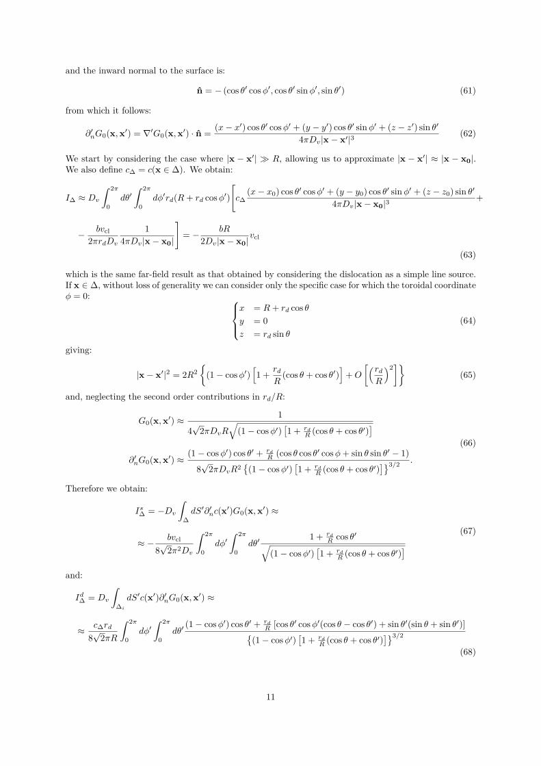
∣∣ also decreases. From a physicalpoint of view the individual vacancy fluxes flowing to (or from) each cavity are reduced by the presenceof a double sink.In a general case of R1 6= R2, we have a more complex situation. Suppose that R2 > R1; then theabsolute value of dR2/dt is monotonically increasing as a function of the inter-cavity distance d.

0.95

0.96

0.97

0.98

0.99

1

1.01

1.02

20 40 60 80 100

Normalized surface velocity

Distance between cavities [nm]

R2=1.5 nm R2=2.0 nm R2=3.0 nm R2=5.0 nm R2=10 nm

Figure 5: Surface velocity of 1 nm spherical cavity as a function of the distance from a second cavity of variable radius,normalized with respect to the case where there is no second cavity. The system is infinite and at a temperature of 1750K, while the bulk vacancy concentration is set to its equilibrium value. Parameters of the model are chosen to describetungsten. Black dots denote the minimum of normalized velocity.

On the other hand, we can define a critical value dc:

dc = R1(c∞ − cΣ1)c∞ − cΣ2

1 +

√1− R2

R1

(c∞ − cΣ2

c∞ − cΣ1

)2 (99)

such that the absolute value of dR1/dt increases with the inter-cavity distance for d > dc and decreasesfor d < dc. In other terms, when the two cavities are sufficiently close, the larger one induces fasterevaporation of the smaller one, in a process which is akin to the well-known Ostwald ripening.

3.5. Validation of the steady-state approximation

The method we described implicitly defines a steady-state concentration field c(x; t) which dependsparametrically on time through ∆i(t), Σj(t) and Se(t). From a physical point of view this means thatvacancy equilibration occurs on much shorter timescales than those related to the macroscopic evolutionof defect clusters. We can now quantitatively validate this assumption a posteriori.Consider a single circular prismatic vacancy loop of radius R inside an infinite medium with a bulkvacancy concentration c∞. The steady-state, or adiabatic, vacancy concentration field c(r; t) at time tand distance r R(t) from the centre of the loop is given by:

c(r; t) = c∞ −bR(t)2Dvr

R(t) = c∞ −πR(t)rln 8R(t)

rd

(c∆(t)− c∞) (100)

where c∆(t) is the vacancy concentration at the dislocation line, which also depends parametrically ontime through R(t). Therefore we can compute the rate of change of the adiabatic vacancy field as:

dc(r; t)dt

= ∂c(r; t)∂R

R(t) = 2π2Dv(c∆(t)− c∞)rb ln 8R(t)

rd

Ωµb c∆(t)4π(1− ν)R(t)kBT

− (c∆(t)− c∞)ln 8R(t)

rd− 1(

ln 8R(t)rd

)2

(101)

18

1e-07

1e-06

1e-05

0.0001

0.001

0.01

0.1

1

10

1 10 100 1000

∆c/c

Distance from source [nm]

R=0.27 nm R=0.60 nm R=1.00 nm R=1.60 nm R=3.20 nm

Figure 6: Relative variation ∆c/c of the vacancy field adiabatic with respect to a circular prismatic vacancy dislocationloop, as a function of the distance r from the vacancy loop, in W. The variation is calculated over a time τ(r) = r2

Dv, i.e.

the approximate equilibration time of perturbations in the vacancy field. Several values of the dislocation loop radius areconsidered. The system temperature is 1750 K and c∞ = c0.

On the other hand, the transient perturbation generated by the dislocation line motion propagates overa distance r in a time of the order of τ(r) ' r2/Dv. We can estimate the relative change in the adiabaticvacancy concentration during a time τ(r) as:

∆c(r; t)c(r; t) '

dc(r; t)dt

τ(r)c(r; t) (102)

Eq.102 provides a quantitative measure that allows us to investigate the regime of applicability of thesteady-state solution. In particular, solving the steady state problem as opposed to the full time-dependent one gives accurate results when ∆c(r; t)/c(r; t) . 1, i.e. when the adiabatic field changesslowly with respect to the propagation of transient perturbations. In Fig.6 we plot the value ∆c/c asa function of r, for several values of the loop radius R, using material parameters for tungsten at atemperature of 1750 K and with c∞ = c0. We can see that for distances less than 20 nm from the loop,the condition of validity is satisfied even for the smallest possible loop size (R = b = 0.27 nm). At largerdistances of 100 nm the condition is not satisfied for loops smaller than approximately 0.60 nm. We pointout, however, that such small loops are typically present in the simulation cell for considerably shortertimescales than the bigger ones, since their climb velocities are exponentially greater. Interstitial loopsand cavities evolve more slowly than vacancy loops, and in addition ∆c/c decreases at lower tempera-tures, therefore we conclude that the steady-state approximation adequately captures the cooperativeevolution of defect clusters in systems of dimensions of the order of hundreds of nanometers.

3.6. Preliminary numerical results

The model in the dilute limit has been implemented numerically in a C++ code that, given an initialstarting configuration of cavities and/or dislocation loops, solves the matrix equation determining in-dividual growth rates, and performs time evolution of the object radii. As previously mentioned, longrange elastic interactions between defects are neglected, and the climb force acting on dislocation loopsis assumed to originate only from elastic self-interaction.The physical parameters required as input are: surface energy density γ (eV/nm2), shear modulus µ(GPa), Poisson’s ratio ν, Burgers vector magnitude b (nm), dislocation core radius rd (nm), atomicvolume Ω (nm3), vacancy formation energy Ev (eV), barrier for vacancy migration Emig (eV), diffusioncoefficient prefactor D0 (nm2/s), and annealing temperature T (K).

19

0.01

0.1

1

10

100

1000

10000

100000

1e+06

1e+07

1400 1500 1600 1700 1800 1900 2000

Annihilation time [s]

T [K]

Object density: 5x10-6 nm-3

Vacancy loops - mixed Interstitial loops - mixed Cavities - mixed Vacancy loops only Interstitial loops only Cavities only

(a)

0.01

0.1

1

10

100

1000

10000

100000

1e+06

1e+07

1400 1500 1600 1700 1800 1900 2000

Annihilation time [s]

T [K]

Object density: 1x10-7 nm-3

Vacancy loops - mixed Interstitial loops - mixed Cavities - mixed Vacancy loops only Interstitial loops only Cavities only

(b)

Figure 7: Total annihilation times in tungsten, as a function of annealing temperature for each object class: 1/2<111>prismatic vacancy loops (red lines) and interstitial loops (yellow lines), and spherical cavities (blue lines). Solid lines wereobtained in the case 10 objects (30 in total) of each class in the simulation cell, while dashed lines were obtained in the caseof 30 objects of the same class. a) The radius of the medium is 111.85 nm and the average object density is 5×10−6 nm−3.b): The radius of the medium is 408.34 nm and the average object density is 1 × 10−7 nm−3. The relevant simulationparameters are: shear modulus µ = 161 Gpa, Poisson’s ratio ν = 0.28, Burgers vector b = 0.274 nm, dislocation core radiusrd = 0.316 nm, atomic volume Ω = 0.016 nm3, vacancy formation energy Ev = 3.65 eV and barrier for vacancy migrationEmig = 1.78 eV. The radii of the defects are normally distributed: with mean 3.2 nm and standard deviation 1 nm, in thecase of dislocation loops, and with mean 1 nm and standard deviation 0.1 nm, in the case of cavities.

The integration time-step is dynamically updated in order to enforce the condition:

10−4 ≤ max1<i<N+M

∣∣dRidt

∣∣Ri

≤ 10−3 (103)

which has been found to give an adequate balance between numerical stability and computational times.Fig.7 shows data obtained using realistic parameters and object distributions, in the case of tungsten. Aset of 10 vacancy dislocation loops, 10 interstitial loops and 10 cavities were randomly distributed insidea spherical medium. Object sizes were sampled from Gaussian distributions with mean 3.2 nm andstandard deviation 1 nm, in the case of dislocation loops, and with mean 1 nm and standard deviation0.1 nm, in the case of cavities. Such size distributions are consistent with the experimentally observabledefects in neutron-irradiated tungsten [5, 3]. The same simulations were repeated in the case of 30objects all of the same type in the simulation cell. In all cases we considered circular prismatic 1

2<111>loops.We have analysed two configurations: one having the defect density of 5 × 10−6 nm−3 and the systemradius of 111.85 nm (Fig.7a), and the other having the defect density of 1× 10−7 nm−3 and the systemradius of 408.34 nm (Fig.7b). Simulations were performed in the temperature range between 1350 K and2000 K. For each object class (i.e. vacancy loops, interstitial loops or cavities) we define an annihilationtime as the time required for every object in the class to disappear. We can immediately note that thetimescales depend exponentially on temperature, which is a feature typical for diffusion-driven dynamics.In particular, by fitting the annihilation time curves to the function:

f(T ) = A

[exp

(E

kBT

)− 1]

(104)

we obtain the average value of parameter E equal to 5.2855 eV, which is remarkably close to the sumEv+Emig = 5.34 eV. More interestingly, the calculated annealing timescales are in quantitative agreementwith experimental data of annealing of dislocation loops in W at ∼ 1670 K [3].When the simulation cell is populated by defect clusters of the same kind, increasing the cluster densityproduces longer annihilation timescales, which is particularly noticeable in the case of vacancy loops. Asthe distances between the defects are reduced, the local environment around each of them will present,on average, higher (in the case of vacancy loops and cavities) or lower (in the case of interstitial loops)

20

vacancy concentrations with respect to the equilibrium value. It can also be noted that this effect ispartially suppressed in the case where clusters of both interstitials and vacancy defects are present inthe simulation cell.This particular example highlights the fact that both defect density and defect distribution can influencethe annealing timescales in a non-trivial way. In order to produce accurate quantitative estimates ofannealing timescales, accurate knowledge on the relative abundance of various defect types is required.While it is straightforward to distinguish cavities from dislocation loops experimentally, it is much moredifficult to characterize whether a given dislocation loop is of vacancy or interstitial type. This isespecially true in the case of radiation-induced prismatic loops, which are only a few nanometers across.As a result, there is still no consensus yet on the relative abundance of vacancy and interstitial typeprismatic loops in irradiated materials, particularly in the case of ion irradiated materials. In the caseof W, some experiments report a roughly equal number of vacancy and interstitial 1

2<111> loops [27],while others report a higher abundance of interstitial loops [28].

4. Conclusions

In this paper we derived an extension of the non-local model for dislocation climb of Gu et al. [1] tothe case of a finite medium with cavities. We also presented a simplified formulation for the case of adilute concentration of spherical cavities and circular prismatic loops. We have shown that the simplifiedmodel adequately predicts the timescales characterizing annealing of radiation defects in tungsten. Theneed for an accurate knowledge of the relative abundance of cluster types is highlighted to characteriseprecisely their annealing timescales.

Acknowledgements

IR and SLD were partly funded by the RCUK Energy Programme (grant No. EP/I501045). IR wasalso supported by the EPSRC Centre for Doctoral Training on Theory and Simulation of Materials atImperial College London under grant number EP/L015579/1. This work was carried out within theframework of the EUROfusion Consortium and has received funding from the Euratom research andtraining programme 2014-2018 under grant agreement No. 633053. The views and opinions expressedherein do not necessarily reflect those of the European Commission. APS is grateful to the BlackettLaboratory for the provision of laboratory facilities. The authors would like to thank the referee fordrawing our attention to a preprint of the paper of ref.[23] prior to its publication.

AppendixA. Derivation of Kirchhoff integral representation

Here we present a rigorous derivation of eq.30, adapted from [2]. We start by considering the equation:

Dv∇2c(x) = −ρ(x) x ∈ V (A.1)

AppendixA.1. Field point not belonging to SConsider a fixed field point x /∈ S, and define Vε as the ball of radius ε centred at x, completely includedin V , and let ∂Vε = Sε. By adapting Eq. (28) to the region V − Vε and taking the limit as ε → 0, wehave:

limε→0

∫V−Vε

c(x′)∇′2G0(x,x′)dV ′ − limε→0

∫V−Vε

G0(x,x′)∇′2c(x′)dV ′ =

=∫S

[c(x′)∂′nG0(x,x′)−G0(x,x′)∂′nc(x′)] dS′ + limε→0

∫Sε

[c(x′)∂′nG0(x,x′)−G0(x,x′)∂′nc(x′)] dS′

(A.2)

Since Dv∇′2G0(x,x′) = δ(x − x′) and by construction x 6= x′, the first term on the left hand side isidentically zero.We also have:

limε→0

∫V−Vε

G0(x,x′)∇′2c(x′)dV ′ = − limε→0

∫V−Vε

G0(x,x′)ρ(x′)Dv

dV ′ = −∫V

G0(x,x′)ρ(x′)Dv

dV ′ (A.3)

21

V

S

S0

S

V

x

Figure A.8: Schematic diagram of the sets under consideration. The region V − Vε is shaded in grey.

where ρ(x) in the last step is justified, assuming ρ to be non-singular, by noting that the |x − x′|−1

singularity in G0(x,x′) is directly integrable in all V . Therefore we just need to consider the limits asε→ 0 of the terms:

IdSε(x) =∫Sε

c(x′)∂′nG0(x,x′)dS′

IsSε(x) =∫Sε

G0(x,x′)∂′nc(x′)dS′(A.4)

we can split the term IdSε as:

IdSε =∫Sε

c(x′)∂′nG0(x,x′)dS′ =∫Sε

[c(x′)− c(x)] ∂′nG0(x,x′)dS′ + c(x)∫Sε

∂′nG0(x,x′)dS′ (A.5)

The term ∂′nG0(x,x′) has a singularity of order 2 for x′ = x, If we assume that c(x) satisfies the Höldercondition:

|c(x)− c(x′)| ≤ C|x− x′|α (A.6)

for x′ ∈ Sε and x in the neighbourhood of x′, with C > 0 and 0 < α ≤ 1, then as ε→ 0 the first integralin Eq. (A.5) vanishes.The second integral can be then straightforwardly computed by taking x = 0 and by noting that:

∂′nG(0,x′)∣∣∣∣x′∈Sε

= ∂

∂ε

14πDvε

= − 14πDvε2

(A.7)

so that:IdSε = c(x)

∫Sε

∂′nG0(x,x′)dS′ = − c(x)4πDvε2

∫ 2π

0dφ

∫ π

0ε2 sin θdθ = −c(x)

Dv(A.8)

In a similar way, we can write:

limε→0

IsSε(x) = − 14πDv

limε→0

∫Sε

∂′nc(x′)dS′ = 0 (A.9)

which, assuming that there is no point-like source at x, vanishes due the fact that ∂′nc(x′) is the normalflux of vacancy concentration integrated over a vanishingly small closed surface.Finally, we obtain the equation:

c(x) = −∫V

G0(x,x′)ρ(x′)dV ′ +Dv

∫S

[c(x′)∂′nG0(x,x′)−G0(x,x′)∂′nc(x′)] dS′ (A.10)

AppendixA.2. Field point on S

22

Now consider the case where x ∈ S. Let Bε(x) be the ball of radius ε around x; we define the sets:

Vε = Bε(x) ∩ V

Sε = ∂Vε ∩ S

S′ε = ∂Vε − Sε

(A.11)

as schematically shown in Fig.A.8. We adapt Eq. (28) to the region V − Vε, bounded by (S − Sε) ∪ S′ε,as: ∫

V

G0(x,x′)ρ(x′)Dv

dV ′ = limε→0

∫S−Sε

[c(x′)∂′nG0(x,x′)−G0(x,x′)∂′nc(x′)] dS′+

+ limε→0

∫S′ε

[c(x′)∂′nG0(x,x′)−G0(x,x′)∂′nc(x′)] dS′(A.12)

where the limiting procedure for volume integrals has already been carried out following the considera-tions for the case x /∈ S, leading to the term on the left hand side. Analogously:

limε→0

∫S′ε

c(x′)∂′nG0(x,x′)dS′ = limε→0

∫S′ε

[c(x′)− c(x)] ∂′nG0(x,x′)dS′︸ ︷︷ ︸=0

+c(x) limε→0

∫S′ε

∂′nG0(x,x′)dS′.

(A.13)Provided that S is smooth2 , as ε→ 0 the surface Sε approaches an hemisphere of radius ε centred in x,leading to:

c(x)∫S′ε

∂′nG0(x,x′)dS′ → − c(x)4πDvε2

∫ 2π

0dφ

∫ π2

0ε2 sin θdθ = −c(x)

2Dv(A.14)

Now consider:limε→0

∫S′ε

G0(x,x′)∂′nc(x′)dS′ = − limε→0

14πDvε

∫S′ε

∂′nc(x′)dS′ (A.15)

which vanishes if no source is applied at point x. More generally, even if ρ(x) 6= 0, but provided thatit is not singular (i.e. excluding point-like sources), Poisson’s equation constrains the possible singularbehaviour of ∂′nc(x′) as:

∂′nc(x′)∣∣∣∣x′∈Sε

= Aε−k A ∈ R, 0 ≤ k < 1 (A.16)

leading to:

limε→0

14πDvε

∫S′ε

∂′nc(x′)dS′ = limε→0

14πDvε

∫ 2π

0dφ

∫ π2

0Aε−kε2 sin θdθ = 1

2Dvlimε→0

ε1−k = 0. (A.17)

We are left with a discussion of the terms:

IdS−Sε(x) =∫S−Sε

c(x′)∂′nG0(x,x′)dS′

IsS−Sε(x) =∫S−Sε

G0(x,x′)∂′nc(x′)dS′(A.18)

Consider the term IdS−Sε and let r = |x′ − x|, we can write:

∂′nG0(x,x′) = ∂G0(r)∂r

∂′nr(x,x′) = 14πDvr2 ∂

′nr(x,x′) = (x′ − x) · n(x′)

4πDvr3 (A.19)

2As a matter of fact, we can relax this assumption. In the general case the result of eq.A.14 is given by −α(x)c(x)4πDv

,where α(x) is the solid angle of the infinitesimal surface element of S at point x.

23

but, for (x′−x) sufficiently small, S can be considered (at least) piecewise flat, thus giving (x′−x)·n(x′) =0 and cancelling out the singularity for x′ = x. This implies that limε→0 I

dS−Sε(x) = IdS(x). Finally, the

singularity in IsS−Sε(x), of order r−1, can be directly integrated over S. Therefore we obtain the finalexpression:

c(x)2 = −

∫V

G0(x,x′)ρ(x′)dV ′ +Dv

∫S

[c(x′)∂′nG0(x,x′)−G0(x,x′)∂′nc(x′)] dS′ (A.20)

24

[1] Y. Gu, Y. Xiang, S. S. Quek, D. J. Srolovitz, Three-dimensional formulation of dislocation climb, Journal of theMechanics and Physics of Solids (2015) 1–19.

[2] F. París, J. Cañas, Boundary Element Method, Fundamentals and Applications, 1st Edition, Oxford University Press,1997.

[3] F. Ferroni, X. Yi, K. Arakawa, S. P. Fitzgerald, P. D. Edmondson, S. G. Roberts, High temperature annealing of ionirradiated tungsten, Acta Materialia 90 (2015) 380–393.

[4] E. E. Bloom, Structural materials for fusion reactors, Nuclear Fusion 30 (1990) 1879–1896.[5] W. Van Renterghem, I. Uytdenhouwen, Investigation of the combined effect of neutron irradiation and electron beam

exposure on pure tungsten, Journal of Nuclear Materials 477 (2016) 77–84.[6] K. Fukumoto, M. Iwasaki, Q. Xu, Recovery process of neutron-irradiated vanadium alloys in post-irradiation annealing

treatment, Journal of Nuclear Materials 442 (2013) 360–363.[7] T. Nagasaka, T. Muroga, H. Watanabe, K. Yamasaki, K. Heo, N.-J.and Shinozaki, M. Narui, Recovery of Hardness,

Impact Properties and Microstructure of Neutron-Irradiated Weld Joint of a Fusion Candidate Vanadium Alloy 46(2005) 498–502.

[8] T. S. Byun, J. H. Baek, O. Anderoglu, S. A. Maloy, M. B. Toloczko, Thermal annealing recovery of fracture toughnessin HT9 steel after irradiation to high doses, Journal of Nuclear Materials 449 (2014) 263–272.

[9] M. Rieth, S. L. Dudarev, S. M. Gonzalez De Vicente, J. Aktaa, T. Ahlgren, S. Antusch, D. E. J. Armstrong,M. Balden, N. Baluc, M. F. Barthe, W. W. Basuki, M. Battabyal, C. S. Becquart, D. Blagoeva, H. Boldyryeva,J. Brinkmann, M. Celino, L. Ciupinski, J. B. Correia, A. De Backer, C. Domain, E. Gaganidze, C. García-Rosales,J. Gibson, M. R. Gilbert, S. Giusepponi, B. Gludovatz, H. Greuner, K. Heinola, T. Höschen, A. Hoffmann, N. Hol-stein, F. Koch, W. Krauss, H. Li, S. Lindig, J. Linke, C. Linsmeier, P. López-Ruiz, H. Maier, J. Matejicek, T. P.Mishra, M. Muhammed, A. Muñoz, M. Muzyk, K. Nordlund, D. Nguyen-Manh, J. Opschoor, N. Ordás, T. Palacios,G. Pintsuk, R. Pippan, J. Reiser, J. Riesch, S. G. Roberts, L. Romaner, M. Rosiński, M. Sanchez, W. Schulmeyer,H. Traxler, A. Ureńa, J. G. Van Der Laan, L. Veleva, S. Wahlberg, M. Walter, T. Weber, T. Weitkamp, S. Wurster,M. A. Yar, J. H. You, A. Zivelonghi, Recent progress in research on tungsten materials for nuclear fusion applicationsin Europe, Journal of Nuclear Materials 432 (2013) 482–500.

[10] D. J. Bacon, T. Diaz de la Rubia, Molecular dynamics computer simulations of displacement cascades in metals,Journal of Nuclear Materials 216 (1994) 275–290.

[11] N. M. Ghoniem, Theory of microstructure evolution under fusion neutron irradiation, Journal of Nuclear Materials179-181 (1991) 99–104.

[12] S. L. Dudarev, Inhomogeneous nucleation and growth of cavities in irradiated materials, Physical Review B 62 (2000)9325–9337.

[13] K. Arakawa, K. Ono, M. Isshiki, K. Mimura, M. Uchikoshi, H. Mori, Observation of the one-dimensional diffusion ofnanometer-sized dislocation loops., Science 318 (2007) 956–959.

[14] S. L. Dudarev, M. R. Gilbert, K. Arakawa, H. Mori, Z. Yao, M. L. Jenkins, P. M. Derlet, Langevin model for real-timeBrownian dynamics of interacting nanodefects in irradiated metals, Physical Review B 81 (2010) 1–15.

[15] S. L. Dudarev, K. Arakawa, X. Yi, Z. Yao, M. L. Jenkins, M. R. Gilbert, P. M. Derlet, Spatial ordering of nano-dislocation loops in ion-irradiated materials, Journal of Nuclear Materials 455 (2014) 16–20.

[16] B. Bakó, E. Clouet, L. Dupuy, M. Blétry, Dislocation dynamics simulations with climb: kinetics of dislocation loopcoarsening controlled by bulk diffusion, Philosophical Magazine 91 (2011) 3173–3191. arXiv:1401.6784.

[17] D. Mordehai, E. Clouet, M. Fivel, M. Verdier, Introducing dislocation climb by bulk diffusion in discrete dislocationdynamics, Philosophical Magazine 88 (2008) 899–925.

[18] Y. Xiang, L.-T. Cheng, D. J. Srolovitz, W. E, A level set method for dislocation dynamics, Acta Materialia 51 (2003)5499–5518.

[19] Y. Xiang, D. J. Srolovitz, Dislocation climb effects on particle bypass mechanisms, Philosophical Magazine 86 (2006)3937–3957.

[20] K. M. Miller, P. T. Heald, The lattice distortion around a vacancy in F.C.C. metals, Physica Status Solidi B 67 (1975)569–576.

[21] F. Hofmann, D. Nguyen-Manh, M. R. Gilbert, C. E. Beck, J. K. Eliason, A. A. Maznev, W. Liu, D. E. J. Armstrong,K. A. Nelson, S. L. Dudarev, Lattice swelling and modulus change in a helium-implanted tungsten alloy: X-raymicro-diffraction, surface acoustic wave measurements, and multiscale modelling, Acta Materialia 89 (2015) 352–363.

[22] S. L. Dudarev, Density Functional Theory Models for Radiation Damage, Annual Review of Materials Research 43(2013) 35–61.

[23] S. Jiang, M. Rachh, Y. Xiang, An efficient high order method for dislocation climb in two dimensions, to appear,preprint available at http://www.math.ust.hk/~maxiang/research/climb_secondkind.pdf (2017).

[24] J. P. Hirth, J. Lothe, Theory of dislocations, 2nd Edition, Wiley, New York, 1982.[25] M. R. Gilbert, S. L. Dudarev, P. M. Derlet, D. G. Pettifor, Structure and metastability of mesoscopic vacancy and

interstitial loop defects in iron and tungsten, Journal of Physics: Condensed Matter 20 (2008) 345214.[26] D. N. Beshers, On the Distribution of Impurity Atoms in the Stress Field of a Dislocation, Acta Metallurgica 6 (1958)

521–523.[27] X. Yi, M. L. Jenkins, M. Briceno, S. G. Roberts, Z. Zhou, M. A. Kirk, In situ study of self-ion irradiation damage in

W and W–5Re at 500 °C, Philosophical Magazine 93 (2013) 1715–1738.[28] T. Amino, K. Arakawa, H. Mori, Activation energy for long-range migration of self-interstitial atoms in tungsten

obtained by direct measurement of radiation-induced point-defect clusters, Philosophical Magazine Letters 91 (2011)86–96.

25