
N. Roussopoulos 2007 OLAP & Data Cubing Spring 2007 Nick Roussopoulos [email protected].
28
-
date post
19-Dec-2015 -
Category
Documents
-
view
213 -
download
0
Transcript of N. Roussopoulos 2007 OLAP & Data Cubing Spring 2007 Nick Roussopoulos [email protected].
N. Roussopoulos 2007 Database Management Systems -2-
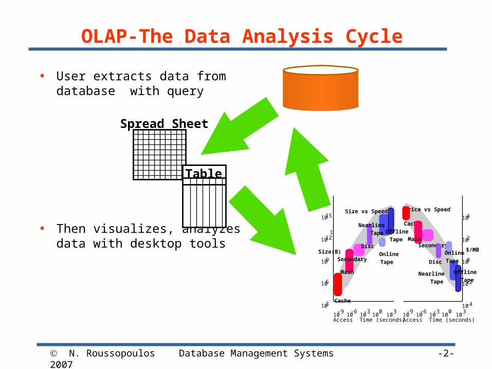
OLAP-The Data Analysis Cycle
• User extracts data from database with query
• Then visualizes, analyzes data with desktop tools
Spread Sheet
Table
1
1015
1012
109
106
103
Size vs Speed
Access Time (seconds)10
-910
-610
-310
010
3
Cache
Main
Secondary
Disc
Nearline
Tape Offline
Tape
Online
Tape
104
102
100
10-2
10-4
Price vs Speed
Access Time (seconds)10
-910
-610
-310
010
3
Cache
MainSecondary
Disc
Nearline
Tape
Offline
Tape
Online
Tape
Size(B) $/MB
N. Roussopoulos 2007 Database Management Systems -3-
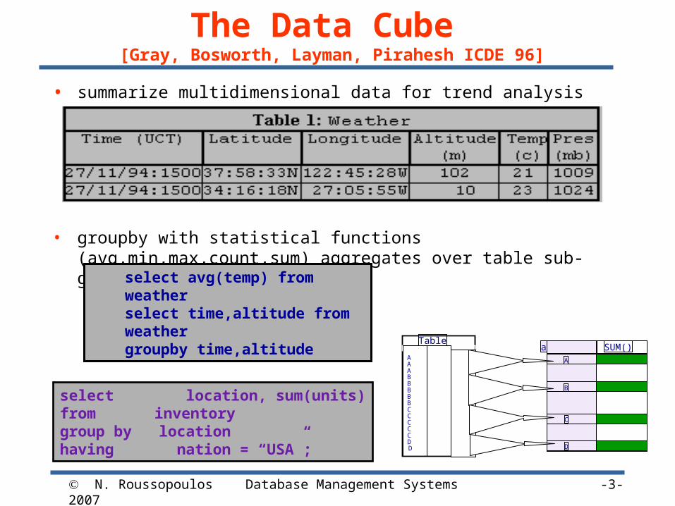
The Data Cube [Gray, Bosworth, Layman, Pirahesh ICDE 96]
• summarize multidimensional data for trend analysis
weather(time,latitude,longitude,altitude,temp,b-pressure)
• groupby with statistical functions (avg,min,max,count,sum) aggregates over table sub-groups
• results in a new table
select location, sum(units)from inventorygroup by locationhaving nation = “USA”;
TableSUM()
A
B
C
D
attributeA A A B B B B B C C C C C D D
select avg(temp) from weatherselect time,altitude from weather groupby time,altitude
N. Roussopoulos 2007 Database Management Systems -4-
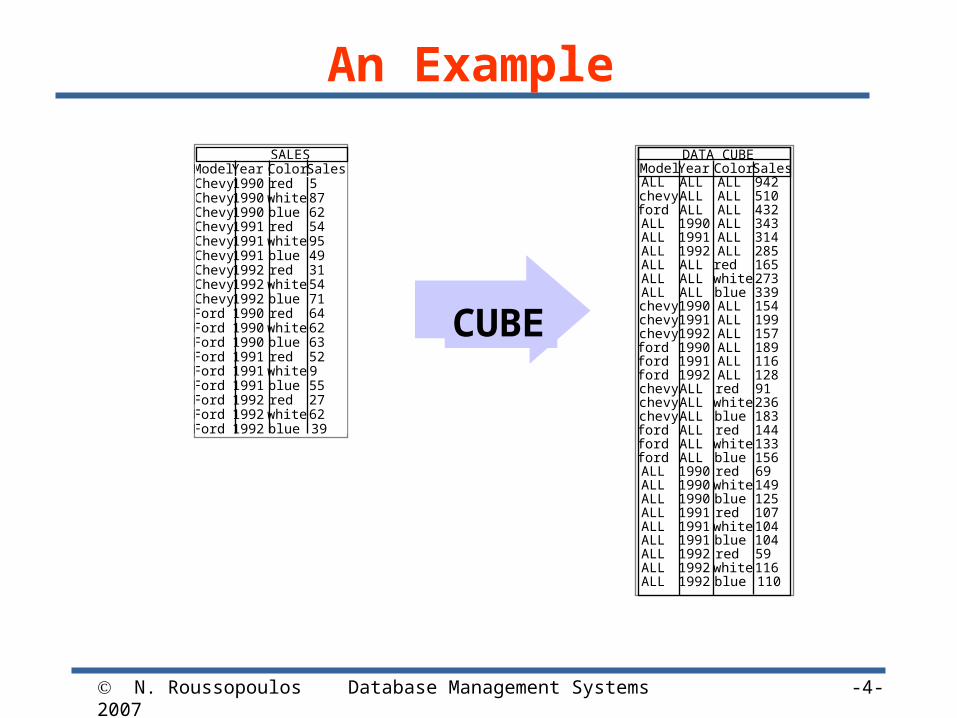
An Example
SALES Model Year Color Sales Chevy 1990 red 5 Chevy 1990 white 87 Chevy 1990 blue 62 Chevy 1991 red 54 Chevy 1991 white 95 Chevy 1991 blue 49 Chevy 1992 red 31 Chevy 1992 white 54 Chevy 1992 blue 71 Ford 1990 red 64 Ford 1990 white 62 Ford 1990 blue 63 Ford 1991 red 52 Ford 1991 white 9 Ford 1991 blue 55 Ford 1992 red 27 Ford 1992 white 62 Ford 1992 blue 39
DATA CUBE Model Year Color Sales ALL ALL ALL 942 chevy ALL ALL 510 ford ALL ALL 432 ALL 1990 ALL 343 ALL 1991 ALL 314 ALL 1992 ALL 285 ALL ALL red 165 ALL ALL white 273 ALL ALL blue 339 chevy 1990 ALL 154 chevy 1991 ALL 199 chevy 1992 ALL 157 ford 1990 ALL 189 ford 1991 ALL 116 ford 1992 ALL 128 chevy ALL red 91 chevy ALL white 236 chevy ALL blue 183 ford ALL red 144 ford ALL white 133 ford ALL blue 156 ALL 1990 red 69 ALL 1990 white 149 ALL 1990 blue 125 ALL 1991 red 107 ALL 1991 white 104 ALL 1991 blue 104 ALL 1992 red 59 ALL 1992 white 116 ALL 1992 blue 110
CUBE
N. Roussopoulos 2007 Database Management Systems -5-
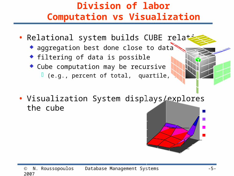
Division of laborComputation vs Visualization
• Relational system builds CUBE relation aggregation best done close to data filtering of data is possible Cube computation may be recursive
(e.g., percent of total, quartile, ....)
• Visualization System displays/explores the cube
19901991
1992ALL
Red
Blue0
50
100
150
200 150-200
100-150
50-100
0-50
N. Roussopoulos 2007 Database Management Systems -6-
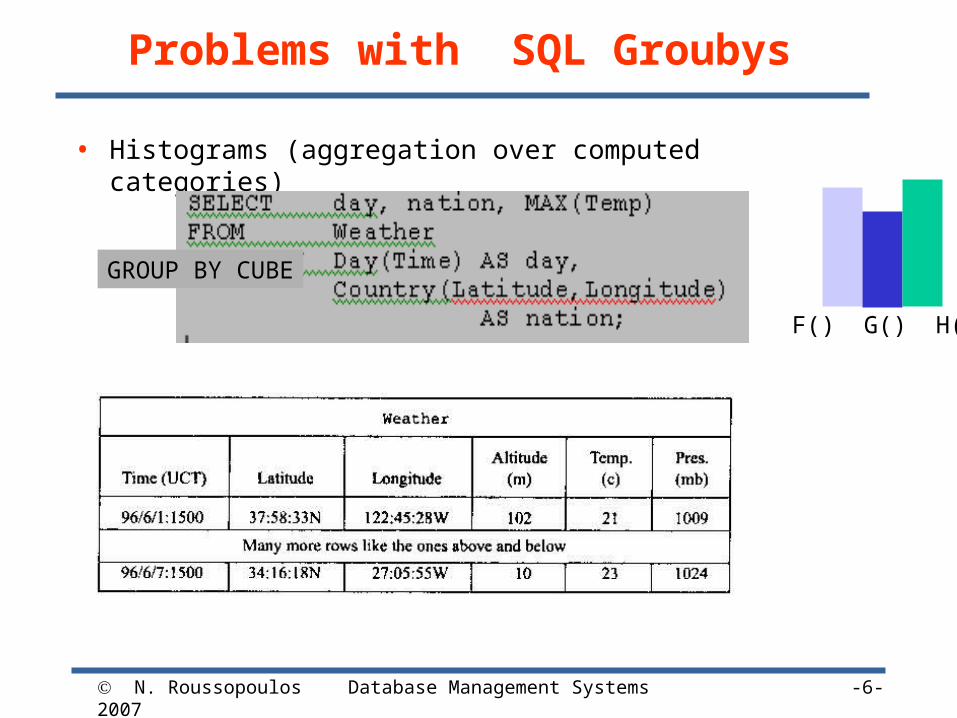
Problems with SQL Groubys
• Histograms (aggregation over computed categories)
F() G() H()
GROUP BY CUBE
N. Roussopoulos 2007 Database Management Systems -7-
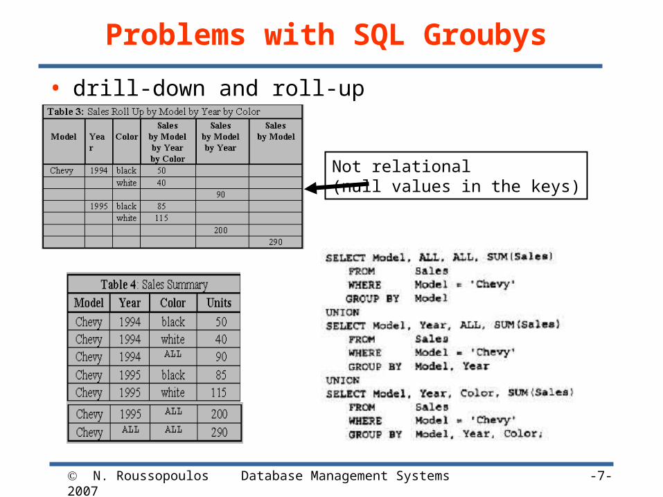
Problems with SQL Groubys
• drill-down and roll-up
Not relational (null values in the keys)
N. Roussopoulos 2007 Database Management Systems -8-
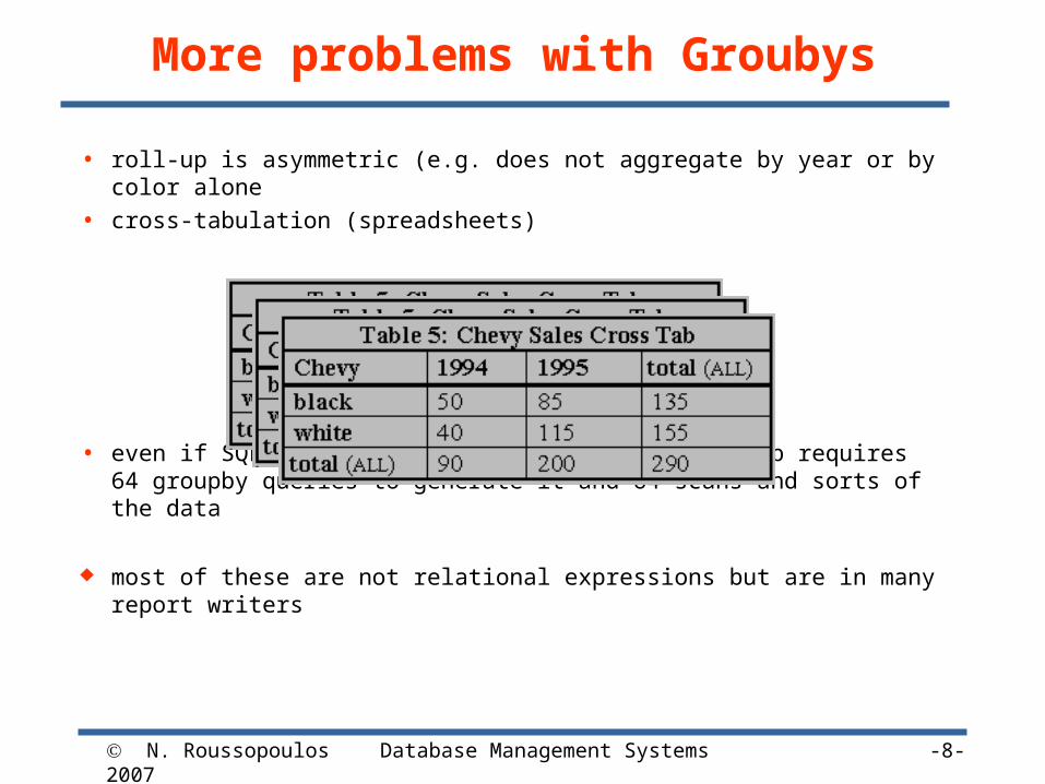
More problems with Groubys
• roll-up is asymmetric (e.g. does not aggregate by year or by color alone
• cross-tabulation (spreadsheets)
• even if SQL syntax can be devised, a 6D cross-tab requires 64 groupby queries to generate it and 64 scans and sorts of the data
most of these are not relational expressions but are in many report writers
N. Roussopoulos 2007 Database Management Systems -9-
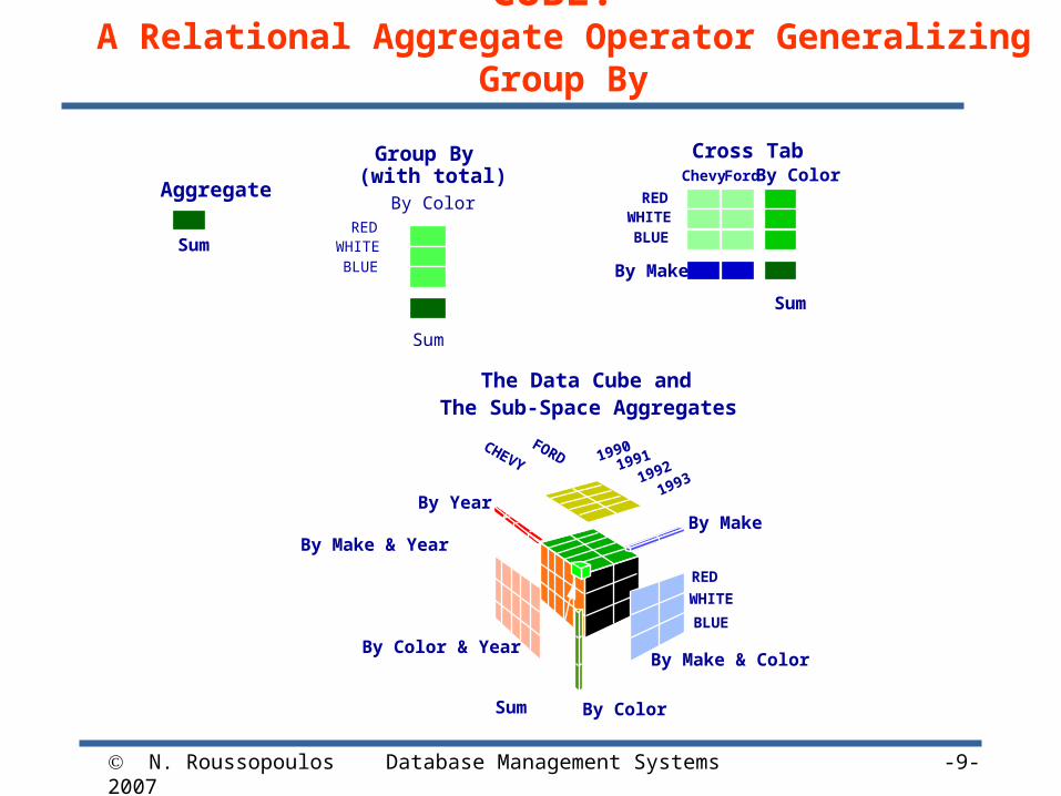
CUBE: A Relational Aggregate Operator Generalizing Group By
By Make & Color
CHEVY
FORD 19901991
1992
1993
RED
WHITE
BLUE
By Color
By Make & Year
By Color & Year
By MakeBy Year
Sum
The Data Cube and The Sub-Space Aggregates
REDWHITEBLUE
ChevyFord
By Make
By Color
Sum
Cross Tab
Sum
Aggregate
REDWHITEBLUE
By Color
Sum
Group By (with total)
N. Roussopoulos 2007 Database Management Systems -10-
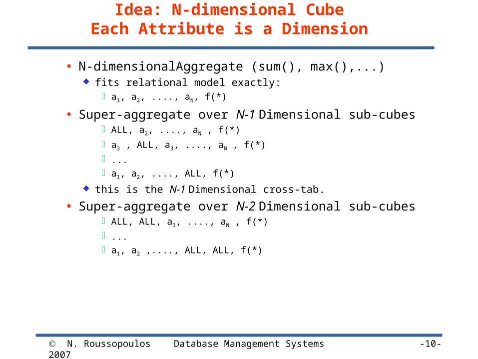
Idea: N-dimensional CubeEach Attribute is a Dimension
• N-dimensionalAggregate (sum(), max(),...) fits relational model exactly:
a1, a2, ...., aN, f(*)
• Super-aggregate over N-1 Dimensional sub-cubesALL, a2, ...., aN , f(*)
a3 , ALL, a3, ...., aN , f(*)
...a1, a2, ...., ALL, f(*)
this is the N-1 Dimensional cross-tab.
• Super-aggregate over N-2 Dimensional sub-cubesALL, ALL, a3, ...., aN , f(*)
...a1, a2 ,...., ALL, ALL, f(*)
N. Roussopoulos 2007 Database Management Systems -11-
Summary of the Cube
• CUBE operator generalizes relational aggregates
• Needs ALL value to denote sub-cubes ALL values represent aggregation sets
• Needs generalization of user-defined aggregates
• Decorations and abstractions are interesting
• Computation has interesting optimizations
• Relationship to “rest of SQL” not fully worked out.
N. Roussopoulos 2007
Computing the (full) Cube
• Discussion from: “Computation of Multi-dimensional Aggregates”; SIGMOD 1996
• Options: One SQL query for each group by on the original data Use one group by to compute another
• e.g., Group-by on (A, B) can be computed from group-bys on (A, B, C) or (A, B, D) etc…
Overlap Method (main contribution of the above paper)• Compute multiple group-by’s simultaneously
• More specifically: For each group-by, can use “sorting” or “hashing” Say (A, B):
• Sorting: Sort the relation first by A, then by B: make a scan and compute the aggregates one by one
• Hashing: Maintain the aggregates (|A| * |B|) in memory – scan the relation once and appropriately update
• What if we want to compute (A, B) from (A, B, C)? If the group-by on (A, B, C) is already sorted, we can do it very efficiently Records (a1, b1, c1, aggr), (a1, b1, c2, aggr) … sequential, so need just one tuple of memory
• What if we want to compute (A, B) from (A, C, B)? This is trickier since all tuples needed to compute (a1, b1, aggr) are not contiguous Need memory equal to |B| tuples
Database Management Systems -12-
N. Roussopoulos 2007
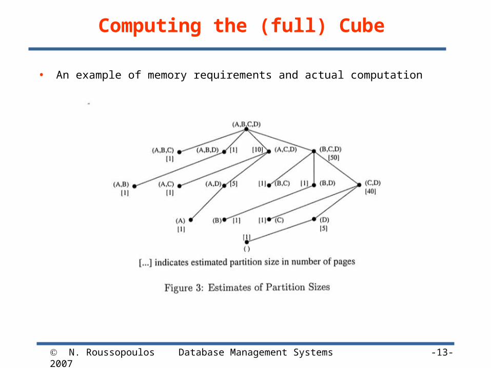
Computing the (full) Cube
• An example of memory requirements and actual computation
Database Management Systems -13-
N. Roussopoulos 2007
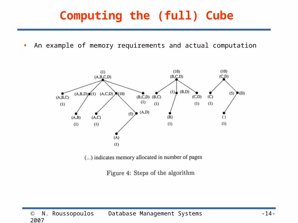
Computing the (full) Cube
• An example of memory requirements and actual computation
Database Management Systems -14-
N. Roussopoulos 2007 Database Management Systems -15-
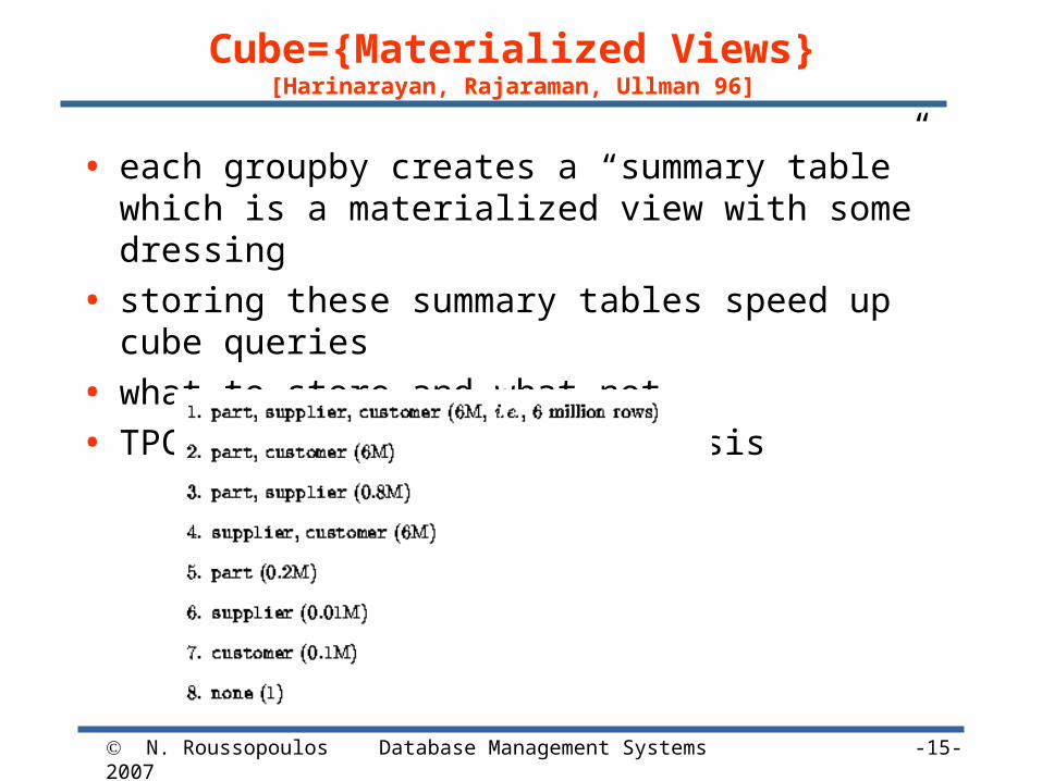
Cube={Materialized Views}[Harinarayan, Rajaraman, Ullman 96]
• each groupby creates a “summary table” which is a materialized view with some dressing
• storing these summary tables speed up cube queries
• what to store and what not
• TPC-D example for sale analysis
N. Roussopoulos 2007 Database Management Systems -16-
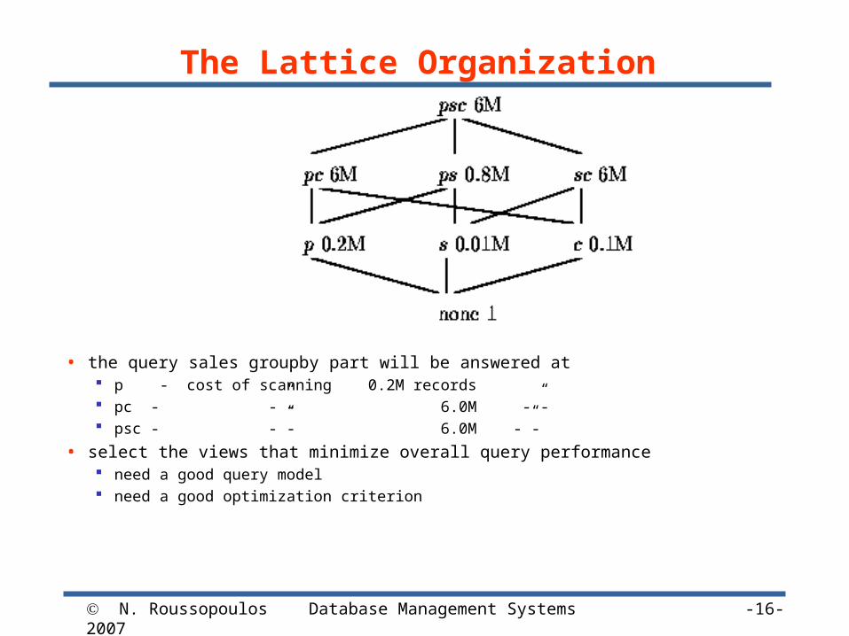
The Lattice Organization
• the query sales groupby part will be answered at p - cost of scanning 0.2M records pc - -”- 6.0M -”- psc - -”- 6.0M -”-
• select the views that minimize overall query performance need a good query model need a good optimization criterion
N. Roussopoulos 2007 Database Management Systems -17-
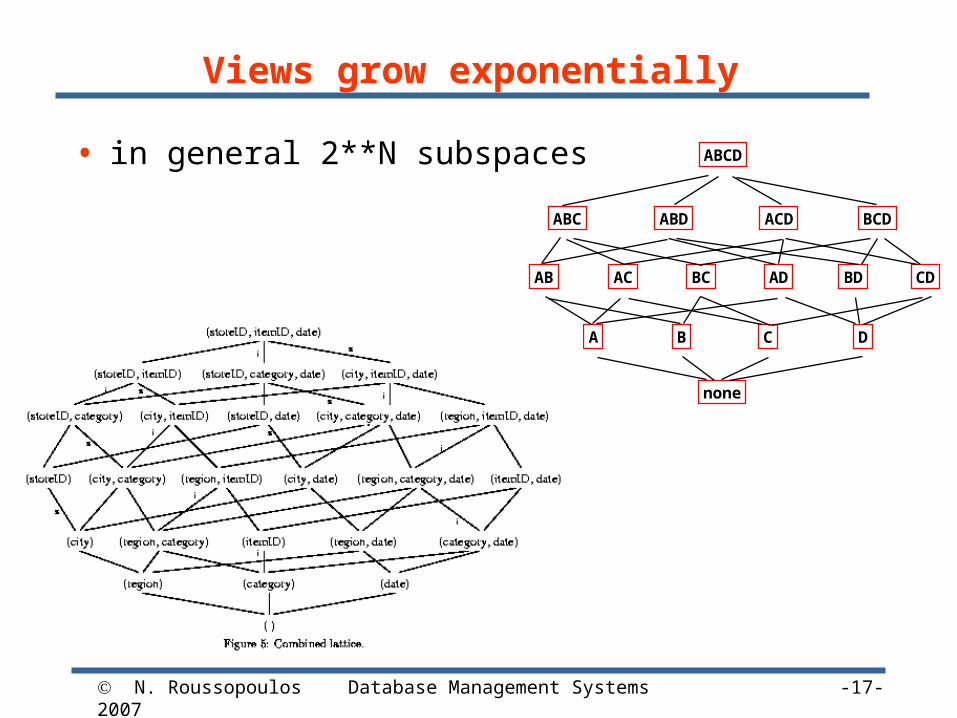
Views grow exponentially
• in general 2**N subspaces ABCD
ABC BCDACDABD
AB ADAC BC BD CD
A B C D
none
N. Roussopoulos 2007 Database Management Systems -18-
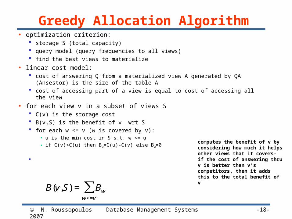
Greedy Allocation Algorithm• optimization criterion:
storage S (total capacity) query model (query frequencies to all views) find the best views to materialize
• linear cost model: cost of answering Q from a materialized view A generated by QA (Ansestor) is the size of
the table A cost of accessing part of a view is equal to cost of accessing all the view
• for each view v in a subset of views S C(v) is the storage cost B(v,S) is the benefit of v wrt S for each w <= v (w is covered by v):
• u is the min cost in S s.t. w <= u
• if C(v)<C(u) then Bw=C(u)-C(v) else Bw=0
€
B(v,S) = Bww<=v
∑
computes the benefit of v by considering how much it helps other views that it covers- if the cost of answering thru v is better than v’s competitors, then it adds this to the total benefit of v
N. Roussopoulos 2007
Greedy Allocation Algorithm
• Can be shown to have an approximation ratio of (1 – 1/e) = 0.63… Seems straightforward application of submodularity of the objective but
did not check carefully
• Issues: Dealing with hierarchies for roll-ups and drill-downs
• Can be incorporated w/o much trouble
Cost of using a view is assumed to be linear• Usually not true
• We may want to build indexes on the views
• Addressed in a later paper by Gupta, Harinarayan, Rajaraman, and Ullman, 1997
Did not look at “refresh time”• Even with batch updates, we still have limited time to do the updates
Database Management Systems -19-
N. Roussopoulos 2007 Database Management Systems -20-
DynaMatYannis Kotidis, Nick Roussopoulos (Sigmod 1999)
• Conventional Data Warehouse pre-computed set view is static (too hard to select and adjust) usually selected by an administrator
• DynaMat proposed a framework for automatic management of views Unifies view selection & view refresh Amortizes generation and maintenance cost over multiple uses of
cached results
• Techniques DynMat caches the results of every query Each incoming query is evaluated against the cached results to see
if any of those can be used The captured set is updated within an update cycle to the extent
possible
N. Roussopoulos 2007 Database Management Systems -21-
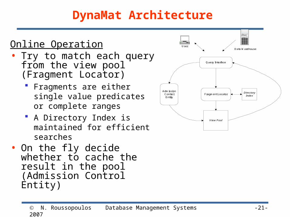
DynaMat Architecture
Query Interface
AdmissionControlEntity
View Pool
DirectoryIndex
Fragment Locator
User
Data General
Data WarehouseOnline Operation• Try to match each query from the
view pool (Fragment Locator) Fragments are either single value
predicates or complete ranges A Directory Index is maintained for
efficient searches
• On the fly decide whether to cache the result in the pool (Admission Control Entity)
N. Roussopoulos 2007 Database Management Systems -22-
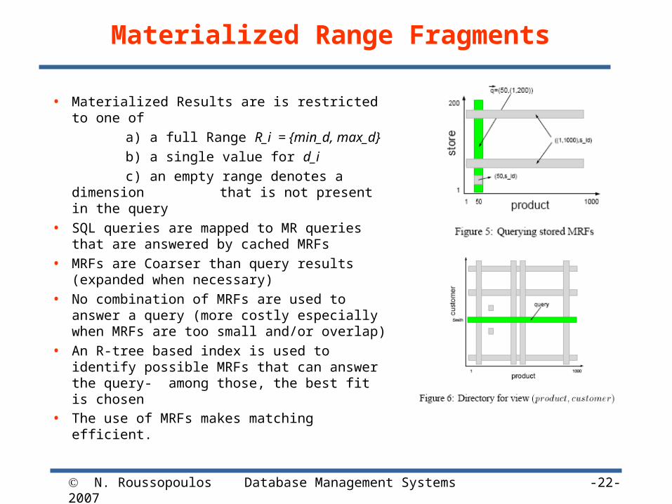
Materialized Range Fragments
• Materialized Results are is restricted to one of
a) a full Range R_i = {min_d, max_d}
b) a single value for d_i
c) an empty range denotes a dimension that is not present in the query
• SQL queries are mapped to MR queries that are answered by cached MRFs
• MRFs are Coarser than query results (expanded when necessary)
• No combination of MRFs are used to answer a query (more costly especially when MRFs are too small and/or overlap)
• An R-tree based index is used to identify possible MRFs that can answer the query- among those, the best fit is chosen
• The use of MRFs makes matching efficient.
N. Roussopoulos 2007 Database Management Systems -23-
Storage Structures & Construction of Cubes
• Subcubes vs. Full cubes Subcube selection
• Cost of construction and indexing
• Maintenance
N. Roussopoulos 2007 Database Management Systems -24-
Cubetrees[Roussopoulos, Kotidis, Roussopoulos 97]
• better storage organization needed materialized views and indexes are not different single storage organization for both
• bulk load techniques are very important rates should be in the order of GB/hour (industrial strength)
• incremental bulk updates is the MOST important issue
• we had lots of experience with spatial access methods: mainly with all possible variations of R-trees (handy)
• packed R-trees
N. Roussopoulos 2007 Database Management Systems -25-
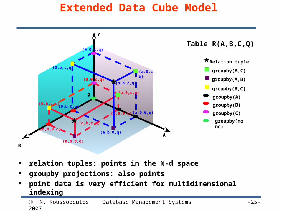
Extended Data Cube Model
Table R(A,B,C,Q)
Relation tuple
groupby(A,C)
groupby(B)
groupby(A,B)
groupby(B,C)
groupby(A)
groupby(C)
groupby(none)
relation tuples: points in the N-d space groupby projections: also points point data is very efficient for multidimensional indexing
C
T(a,b,c,q)
(a,0,0,q)
(a,b,0,q)
(a,0,c,q)
(0,b,0,q)
(a,b,0,q)
T (a,b,c,q)
(a,0,0,q)
(a,0,c,q)
A
B
(0,b,0,q)
(0,b,c,q)
(0,0,c,q)
(0,b,c,q)
0
(0,0,c,q)
N. Roussopoulos 2007 Database Management Systems -26-
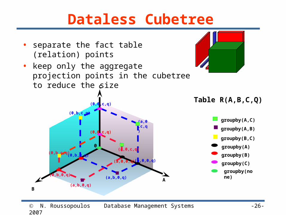
Dataless Cubetree
• separate the fact table (relation) points
• keep only the aggregate projection points in the cubetree to reduce the size
Table R(A,B,C,Q)
groupby(A,C)
groupby(B)
groupby(A,B)
groupby(B,C)
groupby(A)
groupby(C)
groupby(none)
(a,0,0,q)
(a,b,0,q)
(a,0,c,q)
(0,b,0,q)
(a,b,0,q)
(a,0,0,q)
(a,0,c,q)
(0,0,c,q)
A
B
(0,b,0,q)
(0,b,c,q)
(0,0,c,q)
(0,b,c,q)
C
0
N. Roussopoulos 2007 Database Management Systems -27-
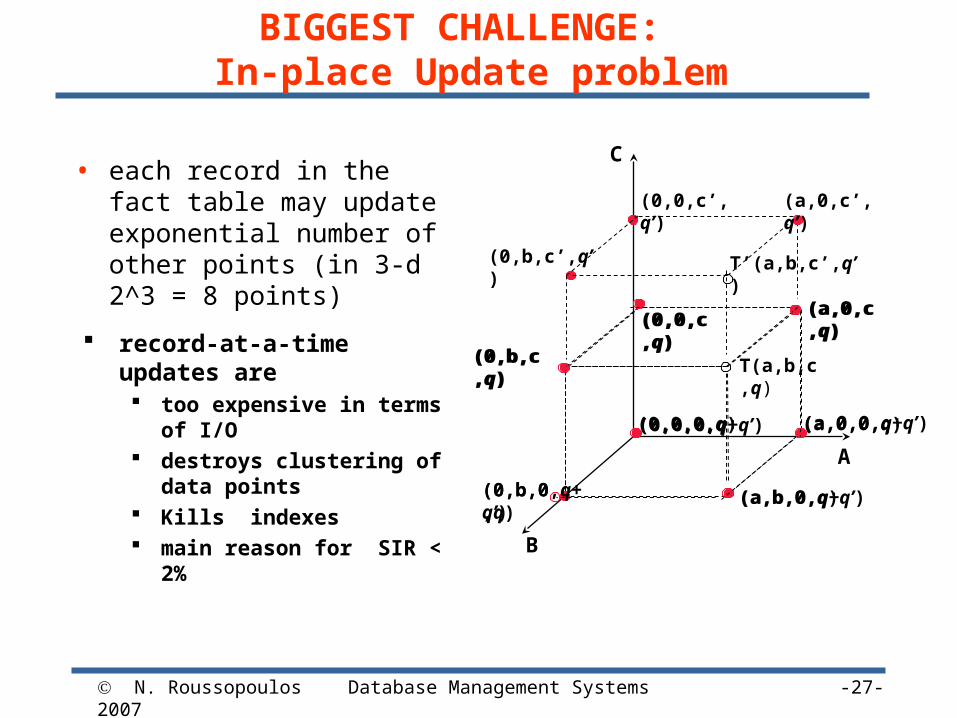
BIGGEST CHALLENGE: In-place Update problem
T(a,b,c,q)
B
C
A
T’(a,b,c’,q’)
(a,0,0,q)
(a,b,0,q)
(0,0,0,q)
(0,b,0,q)
(0,b,c,q)
(a,0,c,q)(0,0,c,q)
(a,0,0,q+q’)
(a,b,0,q+q’)
(0,0,0,q+q’)
(0,b,0,q+q’)
(0,b,c,q)
(a,0,c,q)(0,0,c,q)
(a,0,c’,q’)(0,0,c’,q’)
(0,b,c’,q’)
• each record in the fact table may update exponential number of other points (in 3-d 2^3 = 8 points)
record-at-a-time updates are too expensive in terms of I/O destroys clustering of data points Kills indexes main reason for SIR < 2%
N. Roussopoulos 2007 Database Management Systems -28-
Future of OLAP & Data Cubing
• The big rush to data warehousing has passed and left bitter taste Too costly Did not achieve the promised database integration
• New applications with multi-dimensional data are needed Cost with today’s technology is much less Data integration is not easier and requires hard brain work
• Promising data areas Scientific Security Web