On the complexity of the hybrid proximal extragradient method

for the iterates and the ergodic mean

Renato D.C. Monteiro ∗ B. F. Svaiter †

March 17, 2009 (Revised; April 10, 2010)

Dedicated to Paul Tseng’s life and career

Abstract

In this paper we analyze the iteration-complexity of the hybrid proximal extragradient (HPE)method for finding a zero of a maximal monotone operator recently proposed by Solodov andSvaiter. One of the key points of our analysis is the use of new termination criteria based on theε-enlargement of a maximal monotone operator. The advantage of using these termination criteriais that their definition do not depend on the boundedness of the domain of the operator. We thenshow that Korpelevich’s extragradient method for solving monotone variational inequalities fallsin the framework of the HPE method. As a consequence, using the complexity analysis of theHPE method, we obtain new complexity bounds for Korpelevich’s extragradient method which donot require the feasible set to be bounded, as assumed in a recent paper by Nemirovski. Anotherfeature of our analysis it that the derived iteration-complexity bounds are proportional to thedistance of the initial point to the solution set. The HPE framework is also used to obtain the firstiteration-complexity result for Tseng’s modified forward-backward splitting method for finding azero of the sum of a monotone Lipschitz continuous map with an arbitrary maximal monotoneoperator whose resolvent is assumed to be easily computable. Using also the framework of theHPE method, we study the complexity of a variant of a Newton-type extragradient algorithmproposed by Solodov and Svaiter for finding a zero of a smooth monotone function with Lipschitzcontinuous Jacobian.

1 Introduction

A broad class of optimization, saddle point, equilibrium and variational inequality (VI) problemscan be posed as the monotone inclusion problem, namely: finding x such that 0 ∈ T (x), where T is amaximal monotone point-to-set operator. The proximal point method, proposed by Rockafellar [21],is a classical iterative scheme for solving the MI problem which generates a sequence xk accordingto

xk = (λkT + I)−1(xk−1).∗School of Industrial and Systems Engineering, Georgia Institute of Technology, Atlanta, GA, 30332-0205. (email:

monteiro@isye.gatech.edu). The work of this author was partially supported by NSF Grants CCF-0808863 andCMMI-0900094 and ONR Grant ONR N00014-08-1-0033.

†IMPA, Instituto de Matematica Pura e Aplicada, Rio de Janeiro, RJ, Brasil (email: benar@impa.br). The work ofthis author was partially supported by FAPERJ grants E-26/152.512/2006 and E-26/ 102.821/2008 and CNPq grants303583/2008-8 and 480101/2008-6.

1

It has been used as a generic framework for the design and analysis of several implementable al-gorithms. The classical inexact version of the proximal point method allows for the presence of asequence of summable errors in the above iteration, i.e.:

‖xk − (λkT + I)−1(xk−1)‖ ≤ ek,

∞∑k=1

ek <∞.

Convergence results under the above error condition have been establish in [21] and have been usedin the convergence analysis of other methods that can be recast in the above framework.

New inexact versions of the proximal point method, with relative error criteria were proposed bySolodov and Svaiter [22, 23, 25, 24]. In this paper, we will be concerned with one of these inexactversions of the proximal point method introduced in [22], namely the hybrid proximal extragradient(HPE) method. In contrast to [22], which studies only global convergence of the HPE method, weestablish in this paper its iteration-complexity. One of the key points of our analysis is the use of anew termination criteria based on the ε-enlargement of T introduced in [2]. More specifically, givenε > 0, the algorithm terminates whenever it finds a point y and a pair (v, ε) such that

v ∈ T ε(y), max‖v‖, ε ≤ ε. (1)

For each x, T ε(x) is an outer approximation of T (x) which coincides with T (x) when ε = 0. Hence,for ε = 0 the above termination criterion reduces to the condition that 0 ∈ T (x). The ε-enlargementof maximal monotone operators is a generalization of the ε-subgradient enlargement of the subdif-ferential of a convex function. The advantage of using this termination criterion is that it does notrequire boundedness of the domain of T . Another feature of our analysis it that the derived iterationcomplexity bounds are proportional to the distance of the initial point to the solution set. Resultsof this kind are known for minimization of convex functions but, to the best our knowledge, are newin the context of monotone VI problems (see for example [18]).

We then establish a new result showing that Korpelevich’s extragradient method for solvingVI problems is a special case of the HPE method. This allows us to obtain an O(d0/ε) iterationcomplexity for termination criterion (1), where d0 is the distance of the initial iterate to the solutionset. Since, together with every iterate yk, the method also generates a pair (vk, εk) so that (1) can bechecked, there is no need to assume the feasible set to be bounded or to estimate d0. We also translate(and sometimes strengthen) the above complexity results to the context of monotone VI problemswith linear operators and/or bounded feasible sets, and monotone complementarity problems.

The HPE framework is also used to obtain the first iteration-complexity result for Tseng’s mod-ified forward-backward splitting method [27] for finding a zero of the sum of a monotone Lipschitzcontinuous map with an arbitrary maximal monotone operator whose resolvent is assumed to beeasily computable.

Using also the framework of the HPE method, we study the complexity of a variant of a Newton-type extragradient algorithm proposed in [22] for finding a zero of a smooth monotone function withLipschitz continuous Jacobian.

Previous papers dealing with iteration-complexity analysis of methods for VIs are as follows.In [14], a unifying geometric framework based on the ellipsoid method ideas is presented for VIswith bounded feasible sets and co-coercive (also know as strong-f-monotone) maps. Bundle typemethods for solving VIs with bounded feasible sets and/or bounded variation maps are studied in[6, 12]. Nemirovski [15] studies the complexity of Korpelevich’s extragradient method under the

2

assumption that the feasible set is bounded and an upper bound of its diameter is known. Nesterov[19] proposes a new dual extrapolation algorithm for solving VI problems whose termination dependson the guess of a ball centered at the initial iterate. Finally, asymptotic rate of convergence resultsfor extra-gradient type methods are thoroughly discussed in [7, 10, 26].

This paper is organized as follows. In Section 2, we review the definition and some of thebasic properties of the ε-enlargement of a point-to-set operator and state some new results aboutthe ε-enlargement of a monotone Lispchitz continuous map. Section 3 introduces two notions ofapproximate solutions for the VI problem. It also discusses how the monotone VI problem can beviewed as a special instance of the monotone inclusion problem and interprets the above two notionsof approximate solutions in terms of criterion (1). The HPE method is reviewed in Section 4, whereits general iteration-complexity is also derived. In Section 5, we derive iteration-complexity resultsfor Korpelevich’s extragradient method to obtain different types of approximate solutions, even forthe case of unbounded feasible sets. In Subsections 5.1 and 5.2, we obtain other complexity resultsfor Korpelevich’s method under different assumptions on the function (e.g., linearity) and the feasibleset (e.g., conic and/or bounded set) of the VI problem. In Section 6, we consider a particular versionof Tseng’s modified forward-backward splitting method [27], review the result of [22] that it can beviewed as a particular case of the HPE method, and use this fact to derive, for the first time, itsiteration-complexities for finding different types of approximate solutions. In Section 7, we studythe iteration-complexity of a Newton-type proximal extragradient method for solving a monotonesmooth nonlinear equation. In Section 8, we conclude our main presentation by providing someconcluding remarks. Finally, we review in Appendix A other notions of error measures and discusstheir relationship with the error measures used in the main presentation of the paper.

2 The ε-enlargement

Since our complexity analysis is based on the ε-enlargement of a monotone operator, in this section wegive its definition and review some of its properties. We also derive new results for the ε-enlargementof Lipschitz continuous monotone operators.

A point-to-set operator T : Rn ⇒ Rn is a relation T ⊂ Rn × Rn and

T (x) = v ∈ Rn | (x, v) ∈ T.

Alternatively, one can consider T as a multi-valued function of Rn into the family ℘(Rn) = 2(Rn) ofsubsets of Rn. Regardless of the approach, it is usual to identify T with its graph,

Gr(T ) = (x, v) ∈ Rn × Rn | v ∈ T (x).

An operator T : Rn ⇒ Rn is monotone if

〈v − v, x− x〉 ≥ 0, ∀(x, v), (x, v) ∈ Gr(T ),

and T is maximal monotone if it is monotone and maximal in the family of monotone operators withrespect to the partial order of inclusion, i.e., S : Rn ⇒ Rn monotone and Gr(S) ⊃ Gr(T ) imply thatS = T .

In [2], Burachik, Iusem and Svaiter introduced the ε-enlargement of maximal monotone operators.Here, we extend this concept to a generic point-to-set operator in Rn. Given T : Rn ⇒ Rn and ascalar ε, define T ε : Rn ⇒ Rn as

T ε(x) = v ∈ Rn | 〈x− x, v − v〉 ≥ −ε, ∀x ∈ Rn, ∀v ∈ T (x), ∀x ∈ Rn. (2)

3

We now state a few useful properties of the operator T ε that will be needed in our presentation.

Proposition 2.1. Let T, T ′ : Rn ⇒ Rn. Then,

a) if ε1 ≤ ε2, then T ε1(x) ⊂ T ε2(x) for every x ∈ Rn;

b) T ε(x) + (T ′)ε′(x) ⊂ (T + T ′)ε+ε′(x) for every x ∈ Rn and ε, ε′ ∈ R;

c) T is monotone if, and only if, T ⊂ T 0;

d) T is maximal monotone if, and only if, T = T 0;

e) if T is maximal monotone, (xk, vk, εk) ⊂ Rn×Rn×R+ converges to (x, v, ε), and vk ∈ T εk(xk)for every k, then v ∈ T ε(x).

Proof. Statements (a), (b), (c), and (d) follow directly from definition (2) and the definition of(maximal) monotonicity. For a proof of statement (e), see [4].

We now make two remarks about Proposition 2.1. If T is a monotone operator and ε ≥ 0,it follows from a) and d), that T ε(x) ⊃ T (x) for every x ∈ Rn, and hence that T ε is really anenlargement of T . Moreover, if T is maximal monotone, then e) says that T and T ε coincide whenε = 0.

The ε-enlargement of monotone operators is a generalization of the ε-subdifferential of convexfunctions. Recall that for a function f : Rn → R and scalar ε ≥ 0, the ε-subdifferential of f is theoperator ∂εf : Rn ⇒ Rn defined as

∂εf(x) = v | f(y) ≥ f(x) + 〈y − x, v〉 − ε, ∀y ∈ Rn, ∀x ∈ Rn.

When ε = 0, the operator ∂εf is simply denoted by ∂f and is referred to as the subdifferential of f .The operator ∂f is trivially monotone if f is proper. If f is a proper lower semi-continuous convexfunction, then ∂f is maximal monotone [20]. The conjugate of f is the function f∗ : Rn → R definedas

f∗(s) = supx∈Rn〈s, x〉 − f(x), ∀s ∈ Rn.

The following result lists some useful properties about the ε-subdifferential of a proper convexfunction.

Proposition 2.2. Let f : Rn → R be a proper convex function. Then,

a) ∂εf(x) ⊂ (∂f)ε(x) for any ε ≥ 0 and x ∈ Rn;

b) ∂εf(x) = v |f(x) + f∗(v) ≤ 〈x, v〉+ ε for any ε ≥ 0 and x ∈ Rn;

c) if v ∈ ∂f(x) and f(y) <∞, then v ∈ ∂εf(y), where ε := f(y)− [f(x) + 〈y − x, v〉].

Note that, due to the definition of T ε, the verification of the inclusion v ∈ T ε(x) requires checkingan infinite number of inequalities. This verification is feasible only for specially-structured instancesof operators T . However, it is possible to compute points in the graph of T ε using the following weaktransportation formula [3].

4

Theorem 2.3 ([3, Theorem 2.3]). Suppose that T : Rn ⇒ Rn is maximal monotone. Let xi, vi ∈ Rn

and εi, αi ∈ R+, for i = 1, . . . , k, be such that

vi ∈ T εi(xi), i = 1, . . . , k,

k∑i=1

αi = 1,

and define

x =k∑

i=1

αixi, v =k∑

i=1

αivi, ε =k∑

i=1

αiεi + αi〈xi − x, vi − v〉. (3)

Then, the following statements hold:

a) ε ≥ 0 and v ∈ T ε(x);

b) if, in addition, T = ∂f for some proper lower semi-continuous convex function f and vi ∈∂εif(xi) for i = 1, . . . , k, then v ∈ ∂εf(x).

Whenever necessary, we will identify a map F : Ω ⊂ Rn → Rn with the point-to-set operatorF : Rn ⇒ Rn,

F (x) =

F (x), x ∈ Ω ;∅, otherwise.

The following result is an immediate consequence of Theorem 2.3.

Corollary 2.4. Let a monotone map F : Ω ⊂ Rn → Rn, points x1, . . . , xk ∈ Rn and nonnegativescalars α1, . . . , αk such that

∑ki=1 αi = 1 be given. Define

x :=k∑

i=1

αixi, F :=k∑

i=1

αiF (xi), ε :=k∑

i=1

αi〈xi − x, F (xi)− F 〉. (4)

Then, ε ≥ 0 and F ∈ F ε(x).

Proof. First use Zorn’s Lemma to conclude that there exist a maximal monotone T : Rn ⇒ Rn whichextends F , that is F ⊂ T . To end the proof, apply Theorem 2.3 to T and use the assumption thatit extends F .

Definition 1. For a constant L ≥ 0, the map F : Ω ⊂ Rm → Rn is said to be L-Lipschitz continuouson Ω if ‖F (x)− F (x)‖ ≤ L‖x− x‖ for any x, x ∈ Ω.

Now we are ready to prove that, for a monotone Lipschitz continuous map F defined on thewhole space Rn, the distance between any vector in F ε(x) and F (x) is proportional to

√ε.

Proposition 2.5. If F : Rn → Rn is monotone and L-Lipschitz continuous on Rn, then for everyx ∈ Rn, ε ≥ 0, and v ∈ F ε(x):

‖F (x)− v‖ ≤ 2√

Lε.

5

Proof. Let v ∈ F ε(x) be given. Then, for any x ∈ Rn, we have

〈F (x)− v, x− x〉 = 〈F (x)− v, x− x〉 − 〈F (x)− F (x), x− x〉≥ −ε− ‖F (x)− F (x)‖‖x− x‖ ≥ −ε− L‖x− x‖2,

where the first inequality follows from the definition of F ε and the Cauchy-Schwarz inequality, andthe second one from the assumption that F : Rn → Rn is L-Lipschitz continuous. Specializing thisinequality for x = x + (2L)−1p, where p = v − F (x), we obtain ‖p‖ ≤ 2

√Lε.

Corollary 2.6. Let a monotone map F : Rn → Rn, points x1, . . . , xk ∈ Rn and nonnegative scalarsα1, . . . , αk such that

∑ki=1 αi = 1 be given and define x, F and ε as in Corollary 2.4. Then, ε ≥ 0

and‖F (x)− F‖ ≤ 2

√ε L. (5)

Proof. By Corollary 2.4, we have F ∈ F ε(x), which together with Proposition 2.5 imply that (5)holds.

We observe that when F is an affine (monotone) map, the left hand side of (5) is zero in view of(4). Hence, in this case, the right hand side of (5) is a poor estimate of the error F (x)− F . We willnow develop a better estimate of this error which depends on a certain constant which measures thenonlinearity of a monotone map F .

Definition 2. For a monotone map F : Ω ⊂ Rn → Rn, let Nonl(F ; Ω) be the infimum of all L ≥ 0such that there exist an L-Lipschitz map G and an affine map A such that

F = G +A,

with G and A monotone.

Clearly, if F is a monotone affine map, then Nonl(F ; Rn) = 0. Note also that if F is monotoneand L-Lipschitz on Ω, then Nonl(F ; Ω) ≤ L. We note however that Nonl(F ; Ω) can be much smallerthan L for many relevant instances. For example, if F = G+µA, where µ ≥ 0, A is a monotone affinemap and the map G is monotone and L-Lipschitz on Ω, then we have Nonl(F ; Ω) ≤ L. Hence, inthe latter case, Nonl(F ; Ω) is bounded by a constant which does not depend on µ while the Lipschitzconstant of F converges to ∞ as µ→∞ if A is not constant.

Proposition 2.7. Let a monotone map F : Rn → Rn, points x1, . . . , xk ∈ Rn and nonnegativescalars α1, . . . , αk such that

∑ki=1 αi = 1 be given and define x, F and ε as in Corollary 2.4. Then,

ε ≥ 0 and‖F (x)− F‖ ≤ 2

√εNF . (6)

where NF := Nonl(F ; Rn).

Proof. Suppose that F = G+A where G is an L-Lipschitz monotone map andA is an affine monotonemap. Define

G =∑k

i=1 αiG(xi), εg :=∑k

i=1 αi〈G(xi)− G, xi − x〉,

a =∑k

i=1 αiA(xi), εa :=∑k

i=1 αi〈A(xi)− a, xi − x〉.(7)

6

Since G is a monotone map, it follows from Corollary 2.6 that εg ≥ 0 and ‖G(x) − G‖ ≤ 2√

εgL.Moreover, since A is affine and monotone, we conclude that a = A(x) and εa ≥ 0. Also, noting thatF = G + a and ε = εa + εg ≥ εg, we conclude that

‖F (x)− F‖ =∥∥[G(x) +A(x)]− [G + a]

∥∥ =∥∥G(x)− G

∥∥ ≤ 2√

εgL ≤ 2√

εL.

Bound (6) now follows by noting that NF is the infimum of all L for G and A as above.

3 Approximate solutions of the VI problem

In this section, we introduce two notions of approximate solutions of VI problem. We then discusshow the monotone VI problem can be viewed as a special instance of the monotone inclusion problemand interpret these two notions of approximate solutions for the VI problem in terms of criterion (1).

We assume throughout this section that the following assumptions hold:

A.1) F : Ω ⊂ Rn → Rn is a continuous monotone map;

A.2) X ⊂ Ω is a non-empty closed convex set.

The monotone VI problem with respect to the pair (F,X), denoted by V IP (F,X), consists offinding x∗ such that

x∗ ∈ X, 〈x− x∗, F (x∗)〉 ≥ 0, ∀x ∈ X. (8)

It is well know that, under the above assumptions, condition (8) is equivalent to

x∗ ∈ X, 〈x− x∗, F (x)〉 ≥ 0, ∀x ∈ X. (9)

We will now introduce two notions of approximate solutions of the V IP (F,X) which are essen-tially relaxations of the characterizations (8) and (9) of an exact solution of VI problem.

Definition 3. A point x ∈ X is an ε-strong solution of V IP (F,X) if

θs(x;F ) := supy∈X〈F (x), x− y〉 ≤ ε, (10)

and is an ε-weak solution of V IP (F,X) if

θw(x;F ) := supy∈X〈F (y), x− y〉 ≤ ε. (11)

The functions θs and −θw are referred to as the gap function and the dual gap function, respec-tively, in [5]. Note that, due to the monotonicity of F , we have 0 ≤ θw(·;F ) ≤ θs(·;F ), and henceevery ε-strong solution is also an ε-weak solution.

For VI problems with unbounded feasible sets, the two above notions of approximate solutionsare too strong. For example, if X = Rn, the set of ε-strong solutions agree with the solution set.The following definition relaxes the above notions.

Definition 4. A point x ∈ X is an (ρ, ε)-strong solution (resp., (ρ, ε)-weak solution) of V IP (F,X)if, for some r ∈ Rn such that ‖r‖ ≤ ρ, x is an ε-strong (resp., ε-weak ) solution of V IP (F − r, X),that is

θs(x;F − r) = supy∈X〈F (x)− r, x− y〉 ≤ ε,

(resp., θw(x;F − r) = sup

y∈X〈F (y)− r, x− y〉 ≤ ε

). (12)

Moreover, any such pair (r, ε) will be called a strong residual (resp., weak) residual of x for V IP (F,X).

7

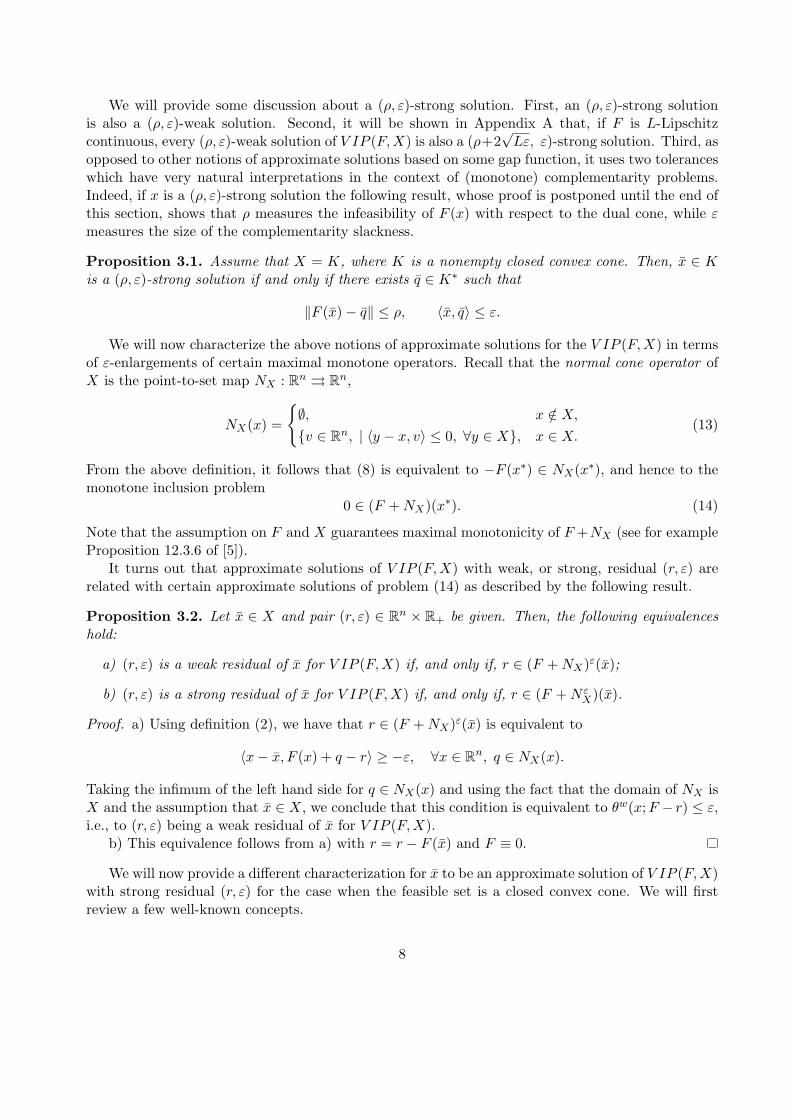
We will provide some discussion about a (ρ, ε)-strong solution. First, an (ρ, ε)-strong solutionis also a (ρ, ε)-weak solution. Second, it will be shown in Appendix A that, if F is L-Lipschitzcontinuous, every (ρ, ε)-weak solution of V IP (F,X) is also a (ρ+2

√Lε, ε)-strong solution. Third, as

opposed to other notions of approximate solutions based on some gap function, it uses two toleranceswhich have very natural interpretations in the context of (monotone) complementarity problems.Indeed, if x is a (ρ, ε)-strong solution the following result, whose proof is postponed until the end ofthis section, shows that ρ measures the infeasibility of F (x) with respect to the dual cone, while εmeasures the size of the complementarity slackness.

Proposition 3.1. Assume that X = K, where K is a nonempty closed convex cone. Then, x ∈ Kis a (ρ, ε)-strong solution if and only if there exists q ∈ K∗ such that

‖F (x)− q‖ ≤ ρ, 〈x, q〉 ≤ ε.

We will now characterize the above notions of approximate solutions for the V IP (F,X) in termsof ε-enlargements of certain maximal monotone operators. Recall that the normal cone operator ofX is the point-to-set map NX : Rn ⇒ Rn,

NX(x) =

∅, x /∈ X,

v ∈ Rn, | 〈y − x, v〉 ≤ 0, ∀y ∈ X, x ∈ X.(13)

From the above definition, it follows that (8) is equivalent to −F (x∗) ∈ NX(x∗), and hence to themonotone inclusion problem

0 ∈ (F + NX)(x∗). (14)

Note that the assumption on F and X guarantees maximal monotonicity of F +NX (see for exampleProposition 12.3.6 of [5]).

It turns out that approximate solutions of V IP (F,X) with weak, or strong, residual (r, ε) arerelated with certain approximate solutions of problem (14) as described by the following result.

Proposition 3.2. Let x ∈ X and pair (r, ε) ∈ Rn × R+ be given. Then, the following equivalenceshold:

a) (r, ε) is a weak residual of x for V IP (F,X) if, and only if, r ∈ (F + NX)ε(x);

b) (r, ε) is a strong residual of x for V IP (F,X) if, and only if, r ∈ (F + N εX)(x).

Proof. a) Using definition (2), we have that r ∈ (F + NX)ε(x) is equivalent to

〈x− x, F (x) + q − r〉 ≥ −ε, ∀x ∈ Rn, q ∈ NX(x).

Taking the infimum of the left hand side for q ∈ NX(x) and using the fact that the domain of NX isX and the assumption that x ∈ X, we conclude that this condition is equivalent to θw(x;F − r) ≤ ε,i.e., to (r, ε) being a weak residual of x for V IP (F,X).

b) This equivalence follows from a) with r = r − F (x) and F ≡ 0.

We will now provide a different characterization for x to be an approximate solution of V IP (F,X)with strong residual (r, ε) for the case when the feasible set is a closed convex cone. We will firstreview a few well-known concepts.

8

The indicator function of X is the function δX : Rn → R defined as

δX(x) =

0, x ∈ X,

∞, otherwise.

The normal cone operator NX of X can be expressed in terms of δX as NX = ∂δX . Direct use ofdefinition (2) and the definition of ε-subdifferential shows that for f = δX , inclusion on Proposi-tion 2.2(a) holds as equality, i.e.:

(NX)ε = ∂εδX . (15)

We now state the following technical result with characterizes membership in (NX)ε in terms ofcertain ε-complementarity conditions.

Lemma 3.3. If K is a nonempty closed convex cone and K∗ is its dual cone, i.e.

K∗ = v ∈ Rn | 〈x, v〉 ≥ 0, ∀x ∈ K,

then, for every x ∈ K, we have

−q ∈ (NK)ε(x) ⇐⇒ q ∈ K∗, 〈x, q〉 ≤ ε .

Proof. Since (NK)ε = ∂εδK , it follows from Proposition 2.2(b) that the condition −q ∈ (NK)ε(x) isequivalent to

(δK)∗(−q) = δK(x) + (δK)∗(−q) ≤ 〈x,−q〉+ ε,

where the first equality follows from the assumption that x ∈ K. To end the proof, it suffices to usethe fact that (δK)∗ = δ−K∗ .

With the aid of the above lemma, we can now give a characterization of strong residuals of feasiblepoints for monotone complementarity problems.

Proposition 3.4. Assume that X = K, where K is a nonempty closed convex cone. Then, (r, ε) isa strong residual of x ∈ K for V IP (F,K) if, and only if,

q := F (x)− r ∈ K∗, 〈x, q〉 ≤ ε.

Proof. This result follows as an immediate consequence of Proposition 3.2(b) and Lemma 3.3.

Finally, note that Proposition 3.1 follows as an immediate consequence of Proposition 3.4.

4 The hybrid proximal extragradient method

Throughout this section, we assume that T : Rn ⇒ Rn is a maximal monotone operator. Themonotone inclusion problem for T is: find x such that

0 ∈ T (x) . (16)

We also assume throughout this section that this problem has a solution, that is, T−1(0) 6= ∅. In thissection we study the iteration complexity of the hybrid proximal extragradient method introducedin [22] for solving the above problem.

9

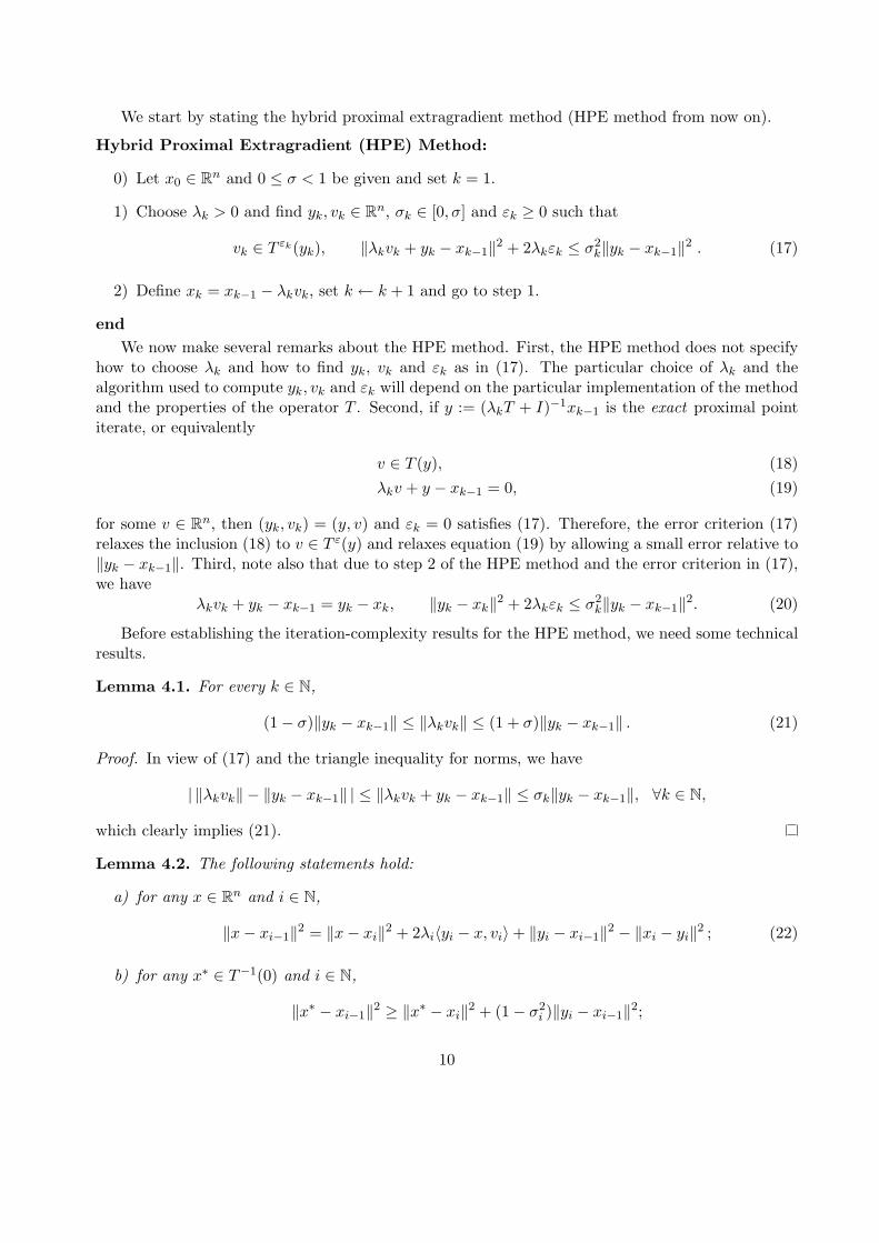
We start by stating the hybrid proximal extragradient method (HPE method from now on).

Hybrid Proximal Extragradient (HPE) Method:

0) Let x0 ∈ Rn and 0 ≤ σ < 1 be given and set k = 1.

1) Choose λk > 0 and find yk, vk ∈ Rn, σk ∈ [0, σ] and εk ≥ 0 such that

vk ∈ T εk(yk), ‖λkvk + yk − xk−1‖2 + 2λkεk ≤ σ2k‖yk − xk−1‖2 . (17)

2) Define xk = xk−1 − λkvk, set k ← k + 1 and go to step 1.

endWe now make several remarks about the HPE method. First, the HPE method does not specify

how to choose λk and how to find yk, vk and εk as in (17). The particular choice of λk and thealgorithm used to compute yk, vk and εk will depend on the particular implementation of the methodand the properties of the operator T . Second, if y := (λkT + I)−1xk−1 is the exact proximal pointiterate, or equivalently

v ∈ T (y), (18)λkv + y − xk−1 = 0, (19)

for some v ∈ Rn, then (yk, vk) = (y, v) and εk = 0 satisfies (17). Therefore, the error criterion (17)relaxes the inclusion (18) to v ∈ T ε(y) and relaxes equation (19) by allowing a small error relative to‖yk − xk−1‖. Third, note also that due to step 2 of the HPE method and the error criterion in (17),we have

λkvk + yk − xk−1 = yk − xk, ‖yk − xk‖2 + 2λkεk ≤ σ2k‖yk − xk−1‖2. (20)

Before establishing the iteration-complexity results for the HPE method, we need some technicalresults.

Lemma 4.1. For every k ∈ N,

(1− σ)‖yk − xk−1‖ ≤ ‖λkvk‖ ≤ (1 + σ)‖yk − xk−1‖ . (21)

Proof. In view of (17) and the triangle inequality for norms, we have

| ‖λkvk‖ − ‖yk − xk−1‖ | ≤ ‖λkvk + yk − xk−1‖ ≤ σk‖yk − xk−1‖, ∀k ∈ N,

which clearly implies (21).

Lemma 4.2. The following statements hold:

a) for any x ∈ Rn and i ∈ N,

‖x− xi−1‖2 = ‖x− xi‖2 + 2λi〈yi − x, vi〉+ ‖yi − xi−1‖2 − ‖xi − yi‖2 ; (22)

b) for any x∗ ∈ T−1(0) and i ∈ N,

‖x∗ − xi−1‖2 ≥ ‖x∗ − xi‖2 + (1− σ2i )‖yi − xi−1‖2;

10

c) for any x∗ ∈ T−1(0), the sequence ‖x∗ − xk‖ is non-increasing and

‖x∗ − x0‖2 ≥∞∑

k=1

(1− σ2k) ‖yk − xk−1‖2 ≥ (1− σ2)

∞∑k=1

‖yk − xk−1‖2 . (23)

Proof. To prove a), let x ∈ Rn and i ∈ N. Then,

‖x− xi−1‖2 = ‖x− xi‖2 + 2〈x− xi, xi − xi−1〉+ ‖xi − xi−1‖2

= ‖x− xi‖2 + 2〈x− yi, xi − xi−1〉+ 2〈yi − xi, xi − xi−1〉+ ‖xi − xi−1‖2

= ‖x− xi‖2 + 2〈x− yi, xi − xi−1〉+ ‖yi − xi−1‖2 − ‖yi − xi‖2.

Statement a) now follows by noting that xi − xi−1 = −λivi, in view of step 2 of the HPE method.If 0 ∈ T (x∗) then, since vi ∈ T εi(yi), the definition of T εk implies that

〈yi − x∗, vi〉 = 〈yi − x∗, vi − 0〉 ≥ −εi.

Using statement a) with x = x∗, the above inequality and (17), we have

‖x∗ − xi−1‖2 ≥ ‖x∗ − xi‖2 − 2λiεi + ‖yi − xi−1‖2 − ‖xi − yi‖2

≥ ‖x∗ − xi‖2 + (1− σ2i )‖yi − xi−1‖2,

which proves b). Statement c) follows immediately from b) and the assumptions 0 ≤ σi ≤ σ < 1 (seesteps 0 and 1 of the HPE method).

Lemma 4.3. Let d0 be the distance of x0 to T−1(0). For every α ∈ R and every k, there exists ani ≤ k such that

‖vi‖ ≤ d0

√√√√(1 + σ)(1− σ)

(λα−2

i∑kj=1 λα

j

), εi ≤

d20σ

2

2(1− σ2)

(λα−1

i∑kj=1 λα

j

). (24)

Proof. Define, for each k ∈ N,

τk := max

2εkλ

1−αk

σ2,‖vk‖2λ2−α

k

(1 + σ)2

.

Then, in view of the assumption that σk ≤ σ for all k ∈ N and relations (17) and (21), we have

τkλαk = max

2εkλk

σ2,λ2

k‖vk‖2

(1 + σ)2

≤ ‖yk − xk−1‖2.

Letting x∗ ∈ T−1(0) be such that d0 = ‖x0−x∗‖, the latter inequality together with (23) then implythat

k∑j=1

τjλαj ≤

k∑j=1

‖yj − xj−1‖2 ≤‖x0 − x∗‖2

(1− σ2)=

d20

(1− σ2),

and hence that (min

j=1,...,kτj

) k∑j=1

λαj ≤

d20

(1− σ2).

The conclusion of the proposition now follows immediately from the latter inequality and the defini-tion of τk.

11

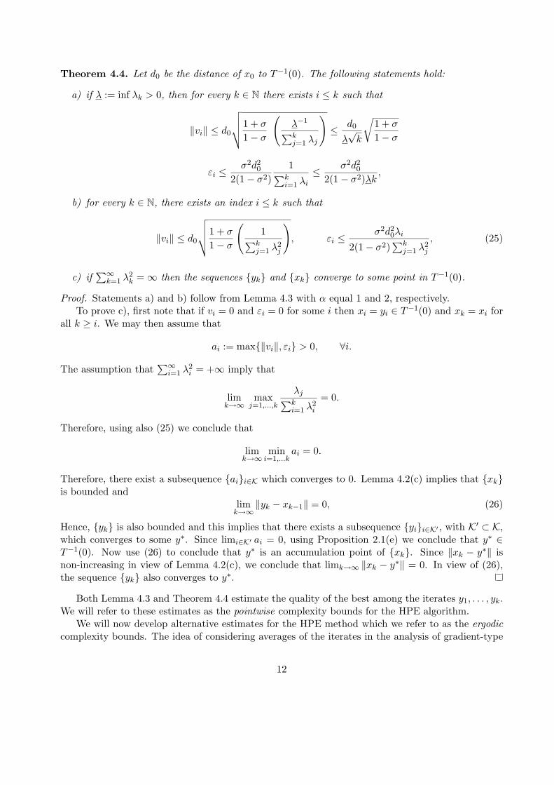
Theorem 4.4. Let d0 be the distance of x0 to T−1(0). The following statements hold:

a) if λ := inf λk > 0, then for every k ∈ N there exists i ≤ k such that

‖vi‖ ≤ d0

√√√√1 + σ

1− σ

(λ−1∑kj=1 λj

)≤ d0

λ√

k

√1 + σ

1− σ

εi ≤σ2d2

0

2(1− σ2)1∑k

i=1 λi

≤ σ2d20

2(1− σ2)λk,

b) for every k ∈ N, there exists an index i ≤ k such that

‖vi‖ ≤ d0

√√√√1 + σ

1− σ

(1∑k

j=1 λ2j

), εi ≤

σ2d20λi

2(1− σ2)∑k

j=1 λ2j

, (25)

c) if∑∞

k=1 λ2k =∞ then the sequences yk and xk converge to some point in T−1(0).

Proof. Statements a) and b) follow from Lemma 4.3 with α equal 1 and 2, respectively.To prove c), first note that if vi = 0 and εi = 0 for some i then xi = yi ∈ T−1(0) and xk = xi for

all k ≥ i. We may then assume that

ai := max‖vi‖, εi > 0, ∀i.

The assumption that∑∞

i=1 λ2i = +∞ imply that

limk→∞

maxj=1,...,k

λj∑ki=1 λ2

i

= 0.

Therefore, using also (25) we conclude that

limk→∞

mini=1,...k

ai = 0.

Therefore, there exist a subsequence aii∈K which converges to 0. Lemma 4.2(c) implies that xkis bounded and

limk→∞

‖yk − xk−1‖ = 0, (26)

Hence, yk is also bounded and this implies that there exists a subsequence yii∈K′ , with K′ ⊂ K,which converges to some y∗. Since limi∈K′ ai = 0, using Proposition 2.1(e) we conclude that y∗ ∈T−1(0). Now use (26) to conclude that y∗ is an accumulation point of xk. Since ‖xk − y∗‖ isnon-increasing in view of Lemma 4.2(c), we conclude that limk→∞ ‖xk − y∗‖ = 0. In view of (26),the sequence yk also converges to y∗.

Both Lemma 4.3 and Theorem 4.4 estimate the quality of the best among the iterates y1, . . . , yk.We will refer to these estimates as the pointwise complexity bounds for the HPE algorithm.

We will now develop alternative estimates for the HPE method which we refer to as the ergodiccomplexity bounds. The idea of considering averages of the iterates in the analysis of gradient-type

12

and/or proximal-point based methods for convex minimization and monotone VIs goes back to atleast the middle seventies (see [1, 13, 17, 16]) and perhaps even earlier.

The sequence of ergodic means yk associated with yk, is defined as

yk :=1Λk

k∑i=1

λiyi, where Λk :=k∑

i=1

λi (27)

The next result, which is a straightforward application of the transportation formula, shows thatthe ergodic iterate is related with the ε-enlargement of T , even when εi ≡ 0. Thus, it provides acomputable residual pair for yk.

Lemma 4.5. For every k ∈ N, define

vk :=1Λk

k∑i=1

λivi, εk :=1Λk

k∑i=1

λi(εi + 〈yi − yk, vi − vk〉). (28)

Then, εk ≥ 0 and vk ∈ T εk(yk).

Proof. The inequality εk ≥ 0 and the inclusion vk ∈ T εk(yk) follow from Theorem 2.3 and theinclusions vi ∈ T εi(yi).

The following result gives alternative expressions for the residual pair (vk, εk), which will be usedfor obtaining bounds on its size.

Proposition 4.6. For any k we have

vk =1Λk

(x0 − xk), (29)

εk =1

2Λk

[2〈yk − x0, xk − x0〉 − ‖xk − x0‖2 + βk

](30)

where

βk :=k∑

i=1

(2λiεi + ‖xi − yi‖2 − ‖yi − xi−1‖2

)≤ 0 . (31)

Proof. The definitions of Λk and vk in (27) and (28) and the update rule in step 2 of the HEP methodimply that

xk = x0 −k∑

i=1

λivi = x0 − Λkvk,

from which (29) follows.Direct use of the definition of yk yields

k∑i=1

λi〈yi − yk, vi − vk〉 =k∑

i=1

λi〈yi − yk, vi〉 −k∑

i=1

λi〈yi − yk, vk〉

=k∑

i=1

λi〈yi − yk, vi〉 −

⟨k∑

i=1

λi(yi − yk), vk

⟩=

k∑i=1

λi〈yi − yk, vi〉 .

13

Adding (22) with x = yk from i = 1 to k, we have

‖yk − x0‖2 = ‖yk − xk‖2 +k∑

i=1

(2λi〈yi − yk, vi〉+ ‖yi − xi−1‖2 − ‖xi − yi‖2

).

Combining the above two equations with the definitions of εk in (28) and βk in (31) we obtain

εk =1

2Λk

[‖yk − x0‖2 − ‖yk − xk‖2 + βk

].

Relation (30) now follow from the above equation and the identity

‖yk − xk‖2 = ‖yk − x0‖2 + 2〈yk − x0, x0 − xk〉+ ‖x0 − xk‖2.

Finally, the inequality in (31) is due to (20) and the assumption 0 ≤ σi ≤ σ < 1 (see steps 0 and 1of the HPE method).

The next result provides estimates on the quality measure of the ergodic mean yk. It essentiallyshows that the quantities vk and εk appearing in (28) are O(1/Λk).

Theorem 4.7. For every k ∈ N, let Λk, yk, vk and εk be as (27), (28). Then, for every k ∈ N, wehave

‖vk‖ ≤2d0

Λk, εk ≤

2θkd20

Λk, (32)

where d0 is the distance of x0 to T−1(0),

θk := 1 +σ√

τk√(1− σ2)

, τk = maxi=1,...,k

λi

Λk≤ 1. (33)

Proof. Let x∗ ∈ T−1(0) be such that ‖x0 − x∗‖ = d0. Using Lemma 4.2(c), we have ‖xk − x∗‖ ≤ d0,and hence

‖xk − x0‖ ≤ ‖xk − x∗‖+ ‖x∗ − x0‖ ≤ 2d0 , (34)

for every k ∈ N. This, together with (29), yields the first bound in (32). Defining

xk =1Λk

k∑i=1

λixi,

and noting (20), (23), (27), (33) and (34), we have

‖xk − x0‖ ≤

∥∥∥∥∥ 1Λk

k∑i=1

λi(xi − x0)

∥∥∥∥∥ ≤ 1Λk

k∑i=1

λi‖xi − x0‖ ≤ 2d0, (35)

‖yk − xk‖2 ≤1Λk

k∑i=1

λi‖yi − xi‖2 ≤ τk

k∑i=1

‖yi − xi‖2 ≤ σ2τk

k∑i=1

‖yi − xi−1‖2 ≤σ2τkd

20

(1− σ2), (36)

where the first inequalities in the above two relations are due to the convexity of ‖ · ‖ and ‖ · ‖2,respectively. The above two relations together with (33) and the triangular inequality for normsyield

‖yk − x0‖ ≤ ‖yk − xk‖+ ‖xk − x0‖ ≤ σd0

√τk

1− σ2+ 2d0 = (1 + θk) d0.

14

Expressions (30) and (31), Cauchy-Schwarz inequality and the above relation then imply

εk ≤1

2Λk

[−‖xk − x0‖2 + 2‖yk − x0‖ ‖xk − x0‖

]≤ 1

2Λk

[−t2k + 2 (1 + θk) d0 tk

]where tk := ‖xk − x0‖2. Since 0 ≤ tk ≤ 2d0 and θk > 1 by (34) and (33), respectively, it follows thatthe maximum of the right hand side of the above relation, with respect to tk is attained at 2d0. Thisclearly implies the second inequality in (32).

5 Korpelevich’s extragradient method for the monotone VIP

Our main goal in this section is to establish the complexity analysis of Korpelevich’s extragradi-ent method for solving the monotone VI problem over an unbounded feasible set. First, we stateKorpelevich’s extragradient algorithm and show that it can be interpreted as a particular case ofthe HPE method. This allows us to use the results of Section 4 to derive its iteration-complexitiesfor computing different notions of approximate solutions. In Subsection 5.1, we obtain additionaliteration-complexity results under the assumption that F is defined in the whole space Rn (e.g.,when F is linear) and/or X is a closed convex cone. In Subsection 5.2, we state the consequences ofthe aforementioned iteration-complexity results for the case when X is bounded.

Korpelevich’s method, as well as its global convergence proof was presented for the first timein [11]. An unifying global convergence analysis of the proximal point method and Korpelevich’smethod for solving V IP (F, Rn) is presented in [7] using the concept of modified monotone maps.Results showing that Korpelevich’s method converges at a linear rate under strong assumptions onthe VIP are given in [26].

Throughout this section, unless otherwise explicitly mentioned, we assume that the set X ⊂ Rn

and the map F : Ω ⊂ Rn → Rn satisfy the following assumptions:

B.1) X ⊂ Ω is a nonempty closed convex set;

B.2) F is monotone and L-Lipschitz continuous ( on Ω);

B.3) the set of solutions of V IP (F,X) is nonempty.

We start by stating Korpelevich’s extragradient algorithm. The notation PX denotes the projectionoperator onto the set X.

Korpelevich’s extragradient algorithm:

0) Let x0 ∈ X and 0 < σ < 1 be given and set λ = σ/L and k = 1.

1) Computeyk = PX(xk−1 − λF (xk−1)), xk = PX(xk−1 − λF (yk)). (37)

2) Set k ← k + 1 and go to step 1.

endWe observe that assumptions B.1 and B.2 imply that the operator T = F +NX is maximal mono-

tone (see for example Proposition 12.3.6 of [5]). Also, recall that solving V IP (F,X) is equivalent

15

to solving the monotone inclusion problem 0 ∈ T (x), where T = F + NX (see the discussion on theparagraph following Proposition 3.1).

We will now show that Korpelevich’s extragradient algorithm for solving V IP (F,X) can beviewed as a particular case of the HEP method for solving the monotone inclusion problem 0 ∈T (x), and this will allow us to obtain iteration-complexity bounds for Korpelevich’s extragradientalgorithm, without assuming boundedness of the feasible set X.

Theorem 5.1. Let yk and xk be the sequences generated by Korpelevich’s extragradient algorithmand, for each k ∈ N, define

qk =1λ

[xk−1 − λF (yk)− xk] , εk = 〈qk, xk − yk〉, vk = F (yk) + qk. (38)

Then:

a) xk = xk−1 − λvk;

b) qk ∈ ∂εkδX(yk) and vk ∈ (F + N εk

X )(yk) ⊂ (F + NX)εk(yk);

c) ‖λvk + yk − xk−1‖2 + 2λεk ≤ σ2‖yk − xk−1‖2.

As a consequence of the above statements, it follows that Korpelevich’s algorithm is a special case ofthe HPE method.

Proof. Statement a) follows immediately from the definition of qk and vk in (38). Recall that theprojection map PX has the property that

z − PX(z) ∈ NX(PX(z)), ∀z ∈ Rn. (39)

Using this fact together with the definition of xk and qk in (37) and (38), respectively, it follows that

qk ∈ NX(xk) = ∂δX(xk). (40)

The first inclusion in statement b) follows from (40) and Proposition 2.2(c). Using this inclusion,the definition of vk, and identity (15), we obtain

vk = F (yk) + qk ∈ F (yk) + ∂εkδX(yk) = F (yk) + (NX)εk(yk)

⊂ F 0(yk) + (NX)εk(yk) ⊂ (F + NX)εk(yk),

where the two last inclusions follows from the monotonicity of F and statement c) and statement b)(with ε′ = 0) of Proposition 2.1.

To prove statement c), define

pk =1λ

[xk−1 − λF (xk−1)− yk] . (41)

Using this definition, the definition of yk in (37) and (39), we conclude that pk ∈ NX(yk). This fact,together with (38), gives the estimate

εk = 〈qk − pk, xk − yk〉+ 〈pk, xk − yk〉 ≤ 〈qk − pk, xk − yk〉

16

This, together with a), imply that

‖λvk + yk − xk−1‖2 + 2λεk = ‖yk − xk‖2 + 2λεk

≤ ‖xk − yk‖2 + 2λ〈qk − pk, xk − yk〉= ‖λ(qk − pk) + xk − yk‖2 − λ2‖qk − pk‖2

≤ ‖λ(qk − pk) + xk − yk‖2 = ‖λ(F (xk−1)− F (yk))‖2,

where the last equality follows from the definition of qk and pk in (38) and (41). Statement c) followsfrom the previous inequality, the assumption that λ = σ/L and our global assumption that F isL-Lipschitz continuous on X.

The following result establishes the global convergence rate of Korpelevich’s extragradient algo-rithm in terms of the criterion (1) with T = F + NX .

Theorem 5.2. Let yk and xk be the sequences generated by Korpelevich’s extragradient algorithmand let vk and εk be the sequences given by (38). For every k ∈ N, define

vk =1k

k∑i=1

vi, yk =1k

k∑i=1

yi, (42)

εk =1k

k∑i=1

[εi + 〈yi − yk, vi − vk〉] . (43)

Then, for every k ∈ N, the following statements hold:

a) yk is an approximate solution of V IP (F,X) with strong residual (vk, εk), and there exists i ≤ ksuch that

‖vi‖ ≤Ld0

σ

√(1 + σ)k(1− σ)

, εi ≤σLd2

0

2(1− σ2)k;

b) yk is an approximate solution of V IP (F,X) with weak residual (vk, εk), and

‖vk‖ ≤2Ld0

kσ, εk ≤

2Ld20θk

kσ, (44)

where d0 is the distance of x0 to the solution set of V IP (F,X) and

θk := 1 +σ√

k(1− σ2). (45)

Proof. a) By Theorem 5.1(b), we have that vk ∈ (F + N εkX )(yk). Hence, by Proposition 3.2(b),

we conclude that yk is an approximate solution of V IP (F,X) with strong residual (vk, εk). Also,Theorem 5.1 implies that Korpelevich’s extragradient algorithm is a special case of the general HPEmethod of Section 4, where λk = σ/L for all k ∈ N. Hence, the remaining claim in (a) follows fromTheorem 4.4(a) with λ = σ/L.

b) By Theorem 5.1(b) and Lemma 4.5 with T = F +NX , we conclude that vk ∈ (F +NX)εk(yk).In view of Proposition 3.2(a), this implies that yk is an approximate solution of V IP (F,X) withweak residual (vk, εk). The bounds in (44) follow from Theorem 4.7 with T = F +NX and λk = σ/L,and the fact that Λk, τk and θk defined in (27) and (33) are, in this case, equal to kλ/L, 1/k and θk,respectively, where θk is given by (45).

17

Observe that the derived bounds obtained in b) are asymptotically better than the ones obtainedin a). Indeed, while the bounds for εk and εk are O(1/k), the ones for vk and vk are O(1/

√k) and

O(1/k) respectively. However, it should be emphasized that a) describes the quality of the strongresidual of some point among the iterates y1, . . . , yk while b) describes the quality of the weak residualof yk.

The following result, which is an immediate consequence of Theorem 5.2, presents iteration-complexity bounds for Korpelevich’s extragradient algorithm to obtain (ρ, ε)-weak and strong solu-tions of V IP (F,X). For simplicity, we ignore the dependence of these bounds on the parameter σand other universal constants and express them only in terms of L, d0 and the tolerances ρ and ε.

Corollary 5.3. Consider the sequence yk generated by Korpelevich’s extragradient algorithm andthe sequence yk defined as in (42). Then, for every pair of positive scalars (ρ, ε), the followingstatements hold:

a) there exists an index

i = O(

max[Ld2

0

ε,L2d2

0

ρ2

])(46)

such that the iterate yi is an (ρ, ε)-strong solution of V IP (F,X);

b) there exists an index

k0 = O(

max[Ld2

0

ε,Ld0

ρ

])(47)

such that, for any k ≥ k0, the point yk is a (ρ, ε)-weak solution of V IP (F,X);

5.1 Specialized complexity results for computing strong solutions

In this section we will obtain additional complexity results assuming that F is defined in all Rn,and/or that the feasible set is a cone.

We first establish the following preliminary result.

Lemma 5.4. Let yk and xk be the sequences generated by Korpelevich’s extragradient algorithmand let vk, qk and εk be the sequences given by (38). For every k ∈ N, define

Fk =1k

k∑i=1

F (yi), qk =1k

k∑i=1

qi, (48)

ε′k =1k

k∑i=1

〈yi − yk, F (yi)− Fk〉, ε′′k =1k

k∑i=1

[εi + 〈yi − yk, qi − qk〉] . (49)

Then, for every k ∈ N, we have:

Fk ∈ F ε′k(yk), qk ∈ (NX)ε′′k (yk), vk = Fk + qk, (50)εk = ε′k + ε′′k, ε′k, ε′′k ≥ 0. (51)

Proof. Applying Theorem 2.3 with T = F , xi = yi, vi = F (xi), εi = 0 and αi = 1/k for i = 1, . . . , k,we conclude that Fk ∈ F ε′k(yk) and ε′k ≥ 0. Also, it follows from Theorem 5.1(b) and Theorem 2.3with T = NX , xi = yi, vi = qi and αi = 1/k, for i = 1, . . . , k, that qk ∈ (NX)ε′′k (yk) and ε′′k ≥ 0. The

18

identity vk = Fk + qk follows from (42), (48) and the fact that vi = F (yi) + qi, i = 1, . . . , k. Theother identity εk = ε′k + ε′′k now follows from (49) and the fact that vk = Fk + qk and vi = F (yi) + qi,i = 1, . . . , k.

The following result shows that, if F is defined in all Rn, satifies Assumptions B.1-B.3 (andhence is L-Lipschitz continuous on the whole Rn), and NF < L, then the iteration complexity for theergodic point yk to be a (ρ, ε)-strong solution is better than the iteration complexity for the best ofthe iterates among y1, . . . , yk to be a (ρ, ε)-strong solution. Moreover, when F is affine, it is shownthat the dependence on the tolerance ρ of the first complexity is O(1/ρ) while that of the secondcomplexity is O(1/ρ2).

Theorem 5.5 (F defined in all Rn). In addition to Assumptions B.1-B.3, assume that Ω = Rn. Letyk and xk be the sequences generated by Korpelevich’s extragradient algorithm, yk, vk, ε′′kand qk be the sequences defined as in (42), (43) and (48), and define

vk := F (yk) + qk, ∀k ∈ N. (52)

Then, for every k ∈ N, yk is an approximate solution of V IP (F,X) with strong residual (vk, ε′′k) and

the following bounds on ‖vk‖ and ε′′k hold:

ε′′k ≤2Ld2

0θk

kσ, ‖vk‖ ≤

d0

√8θkLNF√kσ

+2Ld0

kσ, (53)

where NF := Nonl(F ; Rn), θk is defined in (45) and d0 is the distance of x0 to the solution set ofV IP (F,X). As a consequence, the following statements hold:

a) for every pair of positive scalars (ρ, ε), there exists an index

k0 = O(

max[Ld2

0

ε,Ld0

ρ+

d20LNF

ρ2

])(54)

such that, for any k ≥ k0, the point yk is a (ρ, ε)-strong solution of V IP (F,X).

c) if F is also affine, then, for every pair of positive scalars (ρ, ε), there exists an index

k0 = O(

max[Ld2

0

ε,Ld0

ρ

])(55)

such that, for any k ≥ k0, the point yk is a (ρ, ε)-strong solution of V IP (F,X).

Proof. a) First note that (52) and (50) imply that vk = F (yk) + qk ∈ (F + Nε′′kX )(yk), from which we

conclude that yk is an approximate solution of V IP (F,X) with strong residual (vk, ε′′k), in view of

Proposition 3.2(b). The first bound in (53) follows immediately from the second bound in (44) andthe fact that ε′′k ≤ εk in view of (51).

Now, (50), (52), Proposition 2.7 with xi = yi and the triangle inequality for norms yield

‖vk‖ ≤ ‖vk‖+ ‖vk − vk‖ = ‖vk‖+ ‖F (yk)− Fk‖ ≤ ‖vk‖+ 2√

εkNF .

The second bound in (53) now follows from the above inequality and the bounds in (44).Statement (a) follows from the bounds in (53), the definition of (ρ, ε)-strong solution and some

straightforward arguments. Statement (b) is a special case of (a) where NF = 0.

19

In many important instances of F (e.g., see the discussion after Definition 2), the constantNF = Nonl(F ; Rn) is much smaller than L, and hence bound (54) can be much smaller than (46) onCorollary 5.3.

In the following result, we consider the situation where X = K is a closed convex cone andV IP (F,K) becomes equivalent to the following monotone complementarity problem:

0 = F (y)− s, 〈y, s〉 = 0, (y, s) ∈ K ×K∗.

Using Proposition 3.4, we can translate the conclusions of Proposition 5.3(a) and Theorem 5.5 tothe context of the above problem as follows.

Corollary 5.6 (Monotone complementarity problems). In addition to Assumptions (B.2)-(B.3),assume that X = K, where K is a nonempty closed convex cone. Consider the sequences xk andyk generated by Korpelevich’s extragradient algorithm applied to V IP (F,K) and the sequencesqk, yk and qk determined according to (38), (42) and (48), respectively. Then, for any pair ofpositive scalars (ρ, ε), the following statements hold:

a) there exists an index

k = O(

max[Ld2

0

ε,L2d2

0

ρ2

])such that the pair (y, s) = (yk,−qk) satisfies

‖F (y)− s‖ ≤ ρ, 〈y, s〉 ≤ ε, (y, s) ∈ K ×K∗; (56)

b) if Ω = Rn and F : Rn → Rn is monotone and L-Lipschitz continuous on Rn, then there existsan index

k0 = O(

max[Ld2

0

ε,Ld0

ρ+

d20LNF

ρ2

]), (57)

where NF := Nonl(F ; Rn), such that, for any k ≥ k0, the pair (y, s) = (yk,−qk) satisfies (56).In particular, if F is affine, then the iteration-complexity bound (57) reduces to the one in (55).

5.2 Bounded Feasible Set

So far, we have obtained complexity results for Korpelevich’s method that do not require boundednessof the feasible set. In this subsection we will give some consequences of these results for the casewhere the feasible set X is bounded.

The following simple result shows that, when X is bounded, every approximate solution ofV IP (F,X) with weak (resp., strong) residual (r, ε) is an ε′-weak (resp., ε′-strong) solution ofV IP (F,X) for some ε′. Recall that the diameter DX of a set X ⊂ R is defined as

DX := sup‖x1 − x2‖ : x1, x2 ∈ X. (58)

Lemma 5.7. Assume that X has finite diameter DX . For any x ∈ X, if (r, ε) ∈ Rn × R+ is aweak (resp., strong) residual of x for V IP (F,X), then x is an ε′-weak (resp., ε′-strong) solution ofV IP (F,X), where

ε′ := ε + supx∈X〈r, x− x〉 ≤ ε + ‖r‖DX .

20

Proof. This result follows from Definitions 3 and 4, the definition of DX and the Cauchy-Schwarzinequality.

The following result derives alternative global convergence rate bounds for Korpelevich’s extra-gradient algorithm in the case where the feasible set X of V IP (F,X) is bounded.

Theorem 5.8 (Bounded feasible sets). Assume that conditions B.1-B.3 hold and that the set X hasfinite diameter

DX <∞.

Consider the sequences xk and yk generated by Korpelevich’s extragradient algorithm applied toV IP (F,X) and the sequences yk and εk determined according to (42) and (43), respectively.Then, for every k ∈ N, the following statements hold:

a) yk is an εk-weak solution of V IP (F,X), or equivalently:

maxx∈X〈F (x), yk − x〉 ≤ εk

whereεk :=

2Ld0

kσ

(DX + d0θk

);

b) if Ω = Rn and F : Rn → Rn is monotone and L-Lipschitz continuous on Rn, then yk is anεk-strong solution of V IP (F,X), or equivalently:

maxx∈X〈F (yk), yk − x〉 ≤ εk

where

εk :=d0DX

√8θkLNF√kσ

+2Ld0(DX + θkd0)

kσ(59)

and NF := Nonl(F ; Rn).

Proof. Both statements follow immediately from Lemma 5.7, Theorem 5.2(b) and Theorem 5.5(a).

The following result, which is an immediate consequence of Theorem 5.8, presents iteration-complexity bounds for Korpelevich’s extragradient algorithm to obtain ε-weak and strong solutionsof V IP (F,X). We again ignore the dependence of these bounds on the parameter σ and otheruniversal constants and express them only in terms of L, d0 and the tolerance ε.

Corollary 5.9. Assume that conditions B.1-B.3 hold and that the set X has finite diameter DX .Consider the sequence yk generated by Korpelevich’s extragradient algorithm applied to V IP (F,X)and the sequence yk determined according to (42). Then, for every ε > 0, the following statementshold:

a) there exists an index

k0 = O(

LDXd0

ε

)(60)

such that, for any k ≥ k0, the point yk is an ε-weak solution of V IP (F,X);

21

b) if Ω = Rn and F : Rn → Rn is monotone and L-Lipschitz continuous on Rn, then there existsan index

k′0 = O(

LDXd0

ε+

LNFD2Xd2

0

ε2

),

where NF := Nonl(F ; Rn), such that, for any k ≥ k′0, the point yk is an ε-strong solution ofV IP (F,X).

It is interesting to compare the iteration-complexity bound obtained in Corollary 5.9(a) for findingan ε-weak solution of V IP (F,X) with the corresponding ones obtained in Nemirovski [15] andNesterov [19]. Indeed, their analysis both yield O(D2

XL/ε) iteration complexity bound to obtainan ε-weak solution of V IP (F,X). Hence, in contrast to their bounds, our bound O(d0DXL/ε) isproportional to d0 and formally shows for the first time that Korpelevich’s extragradient methodbenefits from warm-start.

6 Tseng’s Modified Forward-Backward Splitting Method

In this section, we analyse a special case of Tseng’s modified forward-backward splitting (MF-BS)method [27] for solving the inclusion problem

0 ∈ T (x), T = F + B, (61)

for the particular case where the following conditions hold:

C.1) F : Rn → Rn is monotone and L-Lipschitz continuous;

C.2) B : Rn ⇒ Rn is maximal monotone;

C.3) the solution set of (F + B)−1(0) 6= ∅.

For this problem, an iteration of the general Tseng’s MF-BS method is as follows:

yk = (I + λkB)−1(I − λkF )(xk−1), xk = PY [yk − λk(F (yk)− F (xk−1))],

where Y is a closed convex set such that (F + B)−1(0) ∩ Y 6= ∅ and λk > 0 is such that

λk‖F (yk)− F (xk−1)‖ ≤ σ‖yk − xk−1‖ (62)

with σ ∈ (0, 1). Note that since we are assuming that F is L-Lipschitz continuous, the aboveinequality is satisfied for λk = σ/L. In the following, we will study the iteration-complexity of thespecial case of Tseng’s method where Y = Rn and λk = σ/L for every k.

We now formally state the special case of the MF-BS method studied in this section.

Tseng’s MF-BS method:

0) Let x0 ∈ Rn and 0 < σ < 1 be given and set λ = σ/L and k = 1.

1) Compute

yk = (I + λB)−1(I − λF )(xk−1), xk = yk − λ(F (yk)− F (xk−1)). (63)

2) Set k ← k + 1 and go to step 1.

end

22

The following result was first observed in [22] for the case Dom(B) = Rn. Although the proof ofits extension for an operator B with arbitrary domain is essentially the same, we will include it herefor the sake of completeness.

Proposition 6.1. Let yk and xk be the sequences generated by Tseng’s MF-BS method. Foreach k, define

qk =1λ

(xk−1 − yk)− F (xk−1), (64)

vk = qk + F (yk). (65)

Then:

a) xk = xk−1 − λvk;

b) qk ∈ B(yk) and vk ∈ T (yk) = (F + B)(yk);

c) ‖λvk + yk − xk−1‖2 ≤ σ2‖yk − xk−1‖2.

As a consequence of the above statements, it follows that the special case of Tseng’s MF-BS methoddescribed above is a special case of the HPE method.

Proof. Statement a) follows directly from (64), (65) and the second equation in (63). The firstinclusion in b) follows from (64) and the first equation in (63), while the second inclusion followsfrom the first one and (65). To prove statement c), first use (64), (65) to obtain

λvk + yk − xk−1 = λ(F (yk)− F (xk−1)) (66)

which, together with the assumption of F being L-Lipschitz continuous and the definition of λ, yieldsthe desired result.

Note that, in view of (66), criterion (62) (with λk = λ) is equivalent to statement c) of the abovetheorem. Also, as a consequence of Proposition 6.1, Theorem 4.4, Proposition 4.5 and Theorem 4.7,we have the following iteration-complexity result about Tseng’s MF-BS method.

Theorem 6.2. Consider the sequences yk and xk generated by Tseng’s MF-BS method, and thesequences vk, yk, vk and εk defined as in (64), (65), (42) and (43) with εi ≡ 0. Then:

a) for every ρ > 0, there exists an index

i = O(

L2d20

ρ2

)such that vi ∈ (F + B)(yi) and ‖vi‖ ≤ ρ;

b) for every ρ, ε > 0, there exists an index

k0 = O(

max[Ld2

0

ε,Ld0

ρ

])such that vk ∈ (F + B)εk(yk), ‖vk‖ ≤ ρ and εk ≤ ε for any k ≥ k0.

23

Since V I(F,X) with X ⊂ Rn closed and convex is equivalent to the inclusion problem (61) withB = NX , Tseng’s MF-BS method with B = NX can be used to solve V IP (F,X). In this case, theiteration formula (63) reduces to

yk = PX [xk−1 − λF (xk−1)], xk = yk − λ(F (yk)− F (xk−1)) (67)

Note that, in contrast to Korpelevich method, the above algorithm for solving V IP (F,X) requiresjust one projection per iteration. Moreover, in addition to the trivial specialization of Theorem 6.2to the context of monotone VIs, all the iteration-complexity results of Section 5 hold for Tseng’sMF-BS method with B = NX .

7 Hybrid proximal extragradient for smooth monotone equations

In this section we consider the problem of solving

F (x) = 0, (68)

where F : Rn → Rn satisfies the following conditions:

D.1) F is monotone;

D.2) F is differentiable and its Jacobian F ′ is L1-Lipschitz continuous.

Note that this problem is a special case of V IP (F,X) where X = Rn.Newton Method applied to problem (68), under assumption D.2, has excellent local convergence

properties, provided the starting point is close to a solution x∗ and F ′ is non-singular at x∗. Globalwell-definedness of Newton’s method requires F ′ to be non-singular everywhere on Rn. However,this additional assumption does not guarantee the global convergence of Newton method. A globallyconvergent extrapolation Newton-type method for solving (68) was proposed in [8, 9] (se also [10]).

Solodov and Svaiter [22] proposed the use of Newton method for approximately solving theproximal subproblem at each iteration of the HPE method for problem (68). In this section, we willanalyze the complexity of a variant of this method. Specifically, we will consider the following specialcase of the HPE method.Newton Proximal Extragradient (NPE) Method:

0) Let x0 ∈ Rn and 0 < σ` < σu < 1 be given and set k = 1.

1) If F (xk1) = 0 STOP. Otherwise

2) Compute λk ∈ R and sk ∈ Rn satisfying

(λkF′(xk−1) + I)sk = −λkF (xk−1), (69)

2L1

σ` ≤ λk‖sk‖ ≤2L1

σu, (70)

3) Define yk = xk−1 + sk and xk = xk−1 − λkF (yk), set k ← k + 1 and go to step 1.

end

24

We will assume that F (xk) 6= 0 for k = 0, 1, . . . . The complexity analysis will not be affected bythis assumption, because any assertion about the results after k iterations will be valid, adding thealternative “or the algorithm finds a zero”.

For practical computations, given λk, the step sk shall be computed solving the linear equation

(F ′(xk) + λ−1k I)s = −F (xk)

Note that the direction sk in step 1 of the NPE method is the Newton direction with respect to theproximal point equation λF (x) + λk(x− xk−1) = 0 at the point xk−1. Define, for each k,

σk :=L1

2λk‖sk‖. (71)

We need the following well-known result about differentiable maps with Lipschitz continuousJacobian.

Lemma 7.1. Suppose that G : Rn → Rn is differentiable and its Jacobian G′ is L-Lipschitz contin-uous. Then, for every x, s ∈ Rn, we have

‖G(x + s)−G(x)−G′(x)s‖ ≤ L

2‖s‖2.

We will now establish that the NPE method can be viewed as a special case of the HPE method.

Lemma 7.2. For each k, σ` ≤ σk ≤ σu and

‖λkF (yk) + yk − xk−1‖ ≤ σk‖yk − xk−1‖. (72)

As a consequence, the NPE method is a special case of the HPE method stated in Section 4 withεk = 0, vk = F (yk) and σ = σu.

Proof. The bounds on σk follows directly from (70). Define for each k

Gk(x) := λkF (x) + x− xk−1.

Then, G′k is λkL1-Lipschitz continuous and in view of (69)

G′k(xk−1)sk + Gk(xk−1) = 0.

Therefore, using Lemma 7.1 and (71) we have

‖Gk(yk)‖ = ‖Gk(yk)− [G(xk−1) + G′k(xk−1)sk]‖ ≤

λkL1

2‖sk‖2 = σk‖sk‖,

which, due to the fact that sk = yk − xk−1, proves (72).Now we shall prove that the NPE method is a special case of the HPE method. Using inequality

(72) and the fact that σk ≤ σu, εk = 0 and vk = F (yk) and F = F 0 = F εk , we conclude thatcondition (17) is satisfied with T = F . To end the proof, note that xk = xk−1 − λkvk.

We have seen in Theorems 4.4 and 4.7 that the performance of the HPE method depends onthe sums

∑λi and

∑λ2

i . We now give lower bounds for these quantities in the context of the NPEmethod.

25

Lemma 7.3. The sequence λk of the NPE method satisfies

4β

L21

∞∑i=1

1λ2

i

≤ d20 , (73)

where d0 is the distance of x0 to F−1(0) and β is the minimum value of the function (1− t2)t2 overthe interval [σ`, σu], i.e.:

β := min(1− σ2` )σ

2` , (1− σ2

u)σ2u. (74)

As a consequence, for any k,k∑

i=1

λi ≥2√

β

L1d0k3/2,

k∑i=1

λ2i ≥

4β

L21d

20

k2 . (75)

Proof. Using the definition of yi and (71) we have

‖yi − xi−1‖2 =1λ2

i

(λ2i ‖si‖)2 =

1λ2

i

(2L1

σi

)2

.

Since the NPE method is a particular case of the HPE method (Lemma 7.2), we can combine theabove equation with the first inequality in (23) to conclude that

d20 ≥

4L2

1

∞∑i=1

(1− σ2i )σ

2i

1λ2

i

.

To end the proof of (73) use the inclusion σi ∈ [σ`, σu] and the definition of β.The inequalities in (75) now follow by noting that the minimum value of the functions

∑ki=1 ti

and∑k

i=1 t2i subject to the condition that∑k

i=1 t−2i ≤ C and ti > 0 for i = 1, . . . , k are k3/2/

√C and

k2/C, respectively.

The next result gives the pointwise iteration complexity bound for the NPE method.

Proposition 7.4. Consider the sequence yk generated by the NPE method. Then, for every k ≥ 1,there exists an index i ≤ k such that

‖F (yi)‖ ≤√

1 + σu

1− σu

L1d20

2k√

β,

where β is the constant defined in Lemma 7.3. As a consequence, for any scalar ε > 0, there existsan index

i = O(

L1d20

ε

)such that the iterate yi satisfies ‖F (yi)‖ ≤ ε.

Proof. By Lemma 7.2, the NPE method is a special case of the HPE method where σ = σu and thesequences vk and εk are given by vk = F (yk) and εk = 0 for every k. Hence, it follows fromTheorem 4.4(b) and Lemma 7.3 that, for every k ∈ N, there exists i ≤ k such that

‖F (yi)‖ = ‖vi‖ ≤

√(1 + σu)(1− σu)

d0(∑ki=1 λ2

i

)1/2≤√

1 + σu

1− σu

L1d20

2k√

β.

The last part of the theorem follows immediately from the first one.

26

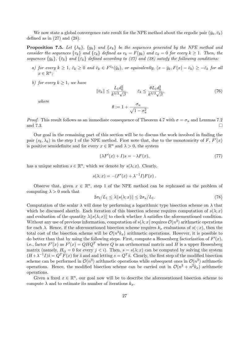
We now state a global convergence rate result for the NPE method about the ergodic pair (yk, vk)defined as in (27) and (28).

Proposition 7.5. Let λk, yk and xk be the sequences generated by the NPE method andconsider the sequences vk and εk defined as vk = F (yk) and εk = 0 for every k ≥ 1. Then, thesequences yk, vk and εk defined according to (27) and (28) satisfy the following conditions:

a) for every k ≥ 1, εk ≥ 0 and vk ∈ F εk(yk), or equivalently, 〈x − yk, F (x) − vk〉 ≥ −εk for allx ∈ Rn;

b) for every k ≥ 1, we have

‖vk‖ ≤L1d

20

k3/2√

β, εk ≤

θL1d30

k3/2√

β, (76)

whereθ := 1 +

σu√1− σ2

u

.

Proof. This result follows as an immediate consequence of Theorem 4.7 with σ = σu and Lemmas 7.2and 7.3.

Our goal in the remaining part of this section will be to discuss the work involved in finding thepair (sk, λk) in the step 1 of the NPE method. First note that, due to the monotonicity of F , F ′(x)is positive semidefinite and for every x ∈ Rn and λ > 0, the system

(λF ′(x) + I)s = −λF (x), (77)

has a unique solution s ∈ Rn, which we denote by s(λ;x). Clearly,

s(λ;x) = −(F ′(x) + λ−1I)F (x) .

Observe that, given x ∈ Rn, step 1 of the NPE method can be rephrased as the problem ofcomputing λ > 0 such that

2σ`/L1 ≤ λ‖s(λ;x)‖ ≤ 2σu/L1. (78)

Computation of the scalar λ will done by performing a logarithmic type bisection scheme on λ thatwhich be discussed shortly. Each iteration of this bisection scheme requires computation of s(λ;x)and evaluation of the quantity λ‖s(λ;x)‖ to check whether λ satisfies the aforementioned condition.Without any use of previous information, computation of s(λ;x) requiresO(n3) arithmetic operationsfor each λ. Hence, if the aforementioned bisection scheme requires kx evaluations of s(·;x), then thetotal cost of the bisection scheme will be O(n3kx) arithmetic operations. However, it is possible todo better than that by using the following steps. First, compute a Hessenberg factorization of F ′(x),i.e., factor F ′(x) as F ′(x) = QHQT where Q is an orthonormal matrix and H is a upper Hessenbergmatrix (namely, Hij = 0 for every j < i). Then, s = s(λ;x) can be computed by solving the system(H+λ−1I)s = QT F (x) for s and and letting s = QT s. Clearly, the first step of the modified bisectionscheme can be performed in O(n3) arithmetic operations while subsequent ones in O(n2) arithmeticoperations. Hence, the modified bisection scheme can be carried out in O(n3 + n2kx) arithmeticoperations.

Given a fixed x ∈ Rn, our goal now will be to describe the aforementioned bisection scheme tocompute λ and to estimate its number of iterations kx.

27

Proposition 7.6. For any x ∈ Rn, the mapping λ→ s(λ;x) is continuous on (0,∞) and

λ‖F (x)‖λ‖F ′(x)‖+ 1

≤ ‖s(λ;x)‖ ≤ λ‖F (x)‖, ∀λ > 0, (79)

where ‖F ′(x)‖ is the operator norm of F ′(x).

Proof. Continuity s(λ) for λ ∈ (0,∞) follows from the fact that F ′(x) is positive semidefinite. Tosimplify the proof, let s = s(λ;x). Using (77), triangle inequality and the definition of operatornorm, we conclude that

λ‖F (x)‖ ≤ ‖λF ′(x)s‖+ ‖s‖ ≤ (‖λF ′(x)‖+ 1)‖s‖,

and hence that the first inequality in (79) holds. To prove the second inequality, we multiply bothsides of (77) by s, use the Cauchy-Schwarz inequality and the positive definiteness of F ′(x) to obtain

‖s‖2 ≤ λ〈s, F ′(x)s〉+ ‖s‖2 = −λ〈s, F (x)〉 ≤ λ‖s‖‖F (x)‖,

and hence that the second inequality in (79) holds.

The following result establishes the existence of scalars λ satisfying (78) under the mild assump-tion that F (x) 6= 0. It also provides an explicit closed interval in R++ which contains all the solutionsof (78). This interval will be used as an initial bracketing interval on a log-type bisection scheme(see Routine Step 1 below) for computing a solution of (78).

Proposition 7.7. Suppose that x ∈ Rn is such that F (x) 6= 0 and let Ix be the set of all λ > 0satisfying (78). Then, Ix is non-empty and Ix ⊂ [ax, bx], where

ax :=

√2σ`

L1‖F (x)‖, bx :=

2σu

L1‖F (x)‖‖F ′(x)‖+

√2σu

L1‖F (x)‖. (80)

Proof. Suppose that x ∈ Rn is such that F (x) 6= 0. By (79) and the fact that F (x) 6= 0, we easilysee that limλ→0 λ‖s(λ;x)‖ = 0 and limλ→∞ λ‖s(λ;x)‖ = ∞. This conclusion together with thecontinuity of the function λ→ λ‖s(λ;x)‖ and the assumption that σ` < σu implies that there existsλ satisfying (78), i.e., Ix 6= ∅.

Assume now that λ ∈ Ix, and hence that (78) holds. The latter relation together with (79) implythat

2σ`

L1≤ λ2‖F (x)‖, λ2‖F (x)‖

λ‖F ′(x)‖+ 1≤ 2σu

L1.

The first inequality clearly implies ax ≤ λ. Multiplying the second inequality by λ‖F ′(x)‖ + 1, weobtain a quadratic inequality in λ which, together with the inequality (α2

1 + α22)

1/2 ≤ α1 + α2 forα1, α2 > 0 imply that λ ≤ bx. We have thus proved that Ix ⊆ [ax, bx].

Lemma 7.8. For every x ∈ Rn such that F (x) 6= 0 and 0 < λ < λ, we have

‖s(λ;x)‖ < ‖s(λ;x)‖ ≤ λ

λ‖s(λ;x)‖. (81)

28

Proof. To simplify the notation, let s = s(λ;x) and s = s(λ;x). Since by definition s(λ;x) is theunique solution of (77), we easily see that

F ′(x)(s− s) = λ−1s− λ−1s. (82)

Noting that s 6= 0 due to Proposition 7.6 and the assumption that F (x) 6= 0, it follows from (82)that s 6= s. Moreover, (82) and the monotonicity of F ′(x) imply that

〈λ−1s− λ−1s, s− s〉 = 〈F ′(x)(s− s), s− s〉 ≥ 0.

Multiplying this inequality by λ λ, we obtain after some straightforward algebraic manipulations that

(λ− λ)〈s, s− s〉 ≥ λ‖s− s‖2.

Since λ−λ > 0 by assumption and s 6= s, the above relation implies that 〈s, s−s〉 > 0, and hence that‖s‖2 > ‖s‖2. This proves the first inequality in (81). Also, the above inequality, the Cauchy-Schwarzinequality and the fact that ‖s− s‖ > 0 imply that

(λ− λ)‖s‖ ≥ λ‖s− s‖.

Adding λ‖s‖ to both sides of this inequality and using the triangle inequality for norms, we obtainthe second inequality in (81).

Corollary 7.9. For every x ∈ Rn such that F (x) 6= 0, the set Ix is a closed interval [λx,`, λx,u] suchthat

λx,u

λx,`≥√

σu

σ`.

Proof. Note that λ→ λ‖s(λ, x)‖ is strictly increasing continuous function over R++ due to the firstinequality in (81). Also, by Proposition 7.6, we have limλ→0 λ‖s(λ;x)‖ = 0 and limλ→∞ λ‖s(λ;x)‖ =∞. The above two observations clearly imply that Ix is a closed interval, say Ix = [λx,`, λx,u], and

λx,`‖s(λx,`;x)‖ =2σ`

L1, λx,u‖s(λx,u;x)‖ =

2σu

L1.

Moreover, the second inequality in (81) implies that

λx,u‖s(λx,u;x)‖ ≤(

λx,u

λx,`

)2

λx,`‖s(λx,`;x)‖.

Combining the above relations, we obtain the desired conclusion.

With the aid of the above results, we can now show how the pair (λk, sk) can be computed atstep 1 of the NPE method. Using xk−1 as input on the following routine, it then output the pair(λk, sk).

29

Routine Step 1:

Input: x ∈ Rn such that F (x) 6= 0 and 0 < σ` < σu < 1;

0) compute ax and bx as in (80) and set a← ax and b← bx;

1) set λ =√

ab and compute s = −(F ′(x) + λ−1I)F (x);

2) if 2σ`/L1 ≤ λ‖s‖ ≤ 2σu/L1, then output the pair (λ, s) and STOP;

3) if λ‖s‖ > 2σu/L1, then set b← λ; otherwise, set a← γ;

4) go to step 1.

endLet ε > 0 be given. We have seen in Proposition 7.4 that the NPE method finds an iterate yi

satisfying the termination criterion ‖F (x)‖ ≤ ε in at most O(L1d20/ε). Clearly, while computing such

an iterate we may assume that ‖F (xk−1)‖ > ε every time step 1 of the NPE method is executed sinceotherwise xk−1 itself would satisfy the termination criterion ‖F (x)‖ ≤ ε. Moreover, (34) implies that‖xk−1 − x0‖ ≤ 2d0. Hence, it is sufficient to analyze the complexity of Routine Step 1 under theassumption that its input x ∈ Rn satisfies ‖F (x)‖ > ε and ‖x − x0‖ ≤ 2d0. In the following result,we also assume that the constants σ` and σu are such that (log σu/σ`)−1 = O(1), which allows us toexpress the complexities only in terms of the quantities L1, ε, d0 and ‖F ′(x0)‖.

Proposition 7.10. Let ε > 0 be given. Then, for every x ∈ Rn such that ‖F (x)‖ > ε and ‖x−x0‖ ≤2d0, the number of iterations and arithmetic operations performed by Routine Step 1 are boundedrespectively by

O(

log log(‖F ′(x0)‖√

L1ε+√

L1√ε

d0

)). (83)

and

O(

n3 + n2 log log(‖F ′(x0)‖√

L1ε+√

L1√ε

d0

)).

Proof. Since log λ = (log a + log b)/2, it follows that, after k inner iterations of the above implemen-tation of step 1 of the NPE method, the scalars a and b at step 3 satisfy

logb

a=

12k

logbx

ax. (84)

Assume now that the method does not stop at the k-th iteration. Then, the values of a and b instep 3 of this iteration satisfy Ix = [λx,`, λx,u] ⊆ [a, b], and hence b/a ≥

√σu/σ`, due to Corollary

7.9. This together with (84) imply that

12k

logbx

ax≥ 1

2log

σu

σ`,

and hence that

k ≤ 1 + log(

log(bx/ax)log(σu/σ`)

).

30

Since (80), Assumption D.2 and the assumption that ‖F (x)‖ > ε and ‖x− x0‖ ≤ 2d0 imply that

bx

ax=√

σu

σ`

(1 +

√2σu

L1‖F (x)‖‖F ′(x)‖

)≤√

σu

σ`

(1 +

√2

L1ε

(‖F ′(x0)‖+ 2L1d0

))we conclude that the number of iterations performed by Routine Step 1 is bounded by (83). Thebound on the number of arithmetic operations is due to the discussion following Proposition 7.5.

8 Concluding Remarks

We provide in this section some concluding remarks.We start by summarizing the contribution of this paper as compared to [22], where the HPE

method was proposed. First, iteration-complexity analysis of the HPE method is given here for thefirst time. Second, in contrast to our analysis, [22] does not study the properties of the ergodicmean for the HPE method. Third, the result that Korpelevich’s method is a special case of the HPEmethod is new. Fourth, in contrast to rule (70), [22] chooses λk proportional to ‖F (xk)‖−1/2 in theNPE method, and does not study the iteration-complexity of the resulting method.

It is important to emphasize that all complexity bounds in Section 5, with the exception of theones obtained in Subsection 5.2, do not require boundedness of the feasible set X. The bounds onthese results are expressed in terms of the distance d0 of the initial point to the solution set, instead ofthe diameter of X. In the usual situation where d0 is unknown, theses complexity bounds have onlytheoretical value in the sense that they can not be used to terminate the method. Instead, our analysisprovides practical stopping rules to obtain (ρ, ε)-weak (resp., -strong) solutions by monitoring thesize of the pair (vk, εk) or the ergodic pair (vk, εk) (or (vk, εk)), both of which can be easily computed.It should be observed that, to obtain an ε-weak/strong solution, it is necessary to have a (finite)bound on the diameter of the feasible set. But as we observed after Definition 4, computation of(ρ, ε)-weak/strong solutions is a natural goal in the context of nonlinear complementarity and mostlikely VI problems as well.

The iteration-complexity analysis developed for the HPE method in this paper was used to obtainiteration-complexity results for two specific algorithms, namely: Korpelevich and NPE methods. Itwould be interesting to derive iteration-complexity results for other algorithms by viewing them asspecial cases of the HPE method.

Appendix

A Relationship between error measures

In this appendix, we review other notions of error measures and discuss their relationship with theerror measures introduced in the main presentation of the paper.

It is well-known that x is a solution of V IP (F,X) if and only if the quantity

rc(x;F ) := c

[x− PX

(x− 1

cF (x)

)](85)

31

vanishes, where c > 0 is a scaling factor. The norm of rc(x;F ) is commonly used to measure thequality of x as an approximate solution of V IP (F,X). Another measure of the quality of x as anapproximate solution of V IP (F,X) is the regularized gap function (see [5]) defined as

θc(x;F ) := supy∈X〈F (x), x− y〉 − c

2‖y − x‖2. (86)

It is easy to see that θc is a nonnegative function whose set of zeros coincides with the solution setof V IP (F,X) and that the unique optimal solution of (86) is

y = PX

(x− 1

cF (x)

).

Hence, in view of (85) we have

θc(x, F ) =1c〈F (x), rc(x;F )〉 − 1

2c‖rc(x;F )‖2. (87)

The following result provides a connection between the regularized gap function and the notion of(ρ, ε)-strong solutions.

Theorem A.1. Let x ∈ X be given. If (r, ε) is a strong residual of x for V IP (F,X), then

θc(x;F ) ≤ 12c‖r‖2 + ε. (88)

Moreover, there exists a unique strong residual (r, ε) of x for which equality holds in (88), namely

r = rc(x;F ), ε =1c

(〈F (x), rc(x;F )〉 − ‖rc(x;F )‖2

). (89)

Proof. Fix x ∈ X. To prove the theorem, it suffices to show, in view of Proposition 3.2(b) and (87),that the solution of the problem

min12c‖r‖2 + ε

s.t. r ∈ (F + N εX)(x)

(90)

is unique and is given by (89). For any r, the smaller ε for which r ∈ F (x) + N ε(x) is given by

supy∈X〈r − F (x), y − x〉.

Hence, problem (90) is equivalent to

minr

supy∈Y

12c‖r‖2 + 〈r − F (x), y − x〉.

Since the above objective function is strongly convex, we conclude that the above problem, and as aby-product problem (90), has a unique optimal solution. Note that (88) follows from the fact that

θc(x;F ) = supy∈Y

infr

12c‖r‖2 + 〈r − F (x), y − x〉 ≤ inf

rsupy∈Y

12c‖r‖2 + 〈r − F (x), y − x〉

32

and the equivalence of the latter problem with (90). Clearly, in view of (89) and (87), it followsthat the objective function of (90) evaluated at the pair (r, ε) given by (89) is equal to θc(x;F ). Toconclude the proof, it suffices to show that this pair also satisfies r ∈ (F + N ε

X)(x). Indeed, using(85), we obtain

PX

(x− 1

cF (x)

)= x− 1

crc(x;F ).

Subtracting F (x) from both sides of (85) and using (39) and the above equation, we conclude that

rc(x;F )− F (x) ∈ NX

(x− 1

crc(x;F )

).

Using the above relation, Proposition 2.2(c) with f = δX , v = rc(x;F )−F (x) and y = x−c−1rc(x;F ),and relation (15), we then conclude that rc(x;F )− F (x) ∈ N ε

X(x) with

ε =⟨

rc(x;F )− F (x) , x− 1crc(x;F )− x

⟩=

1c

(〈F (x), rc(x;F )〉 − ‖rc(x;F )‖2

).

The following result follows as an immediate consequence of the Theorem A.1.

Corollary A.2. Let x ∈ X be given. If x is a (ρ, ε)-strong solution of V IP (F,X), then for anyc > 0,

θc(x;F ) ≤ ρ2

2c+ ε, ‖rc(x;F )‖ ≤

√ρ2 + 2cε.

We now relate the notion of a weak-solution with that of a strong-solution.

Lemma A.3. If F is L-Lipschitz continuous in X, then for any x ∈ X,

θ2L(x;F ) ≤ θw(x;F ).

Proof. Using Definition 3 and the Lipschitz continuity of F , we have

θw(x;F ) = supy∈X〈F (y), x− y〉 = sup

y∈X〈F (x), x− y〉+ 〈F (y)− F (x), x− y〉

≥ supy∈X〈F (x), x− y〉 − L‖x− y‖2 = θ2L(x;F ).

Theorem A.4. If F is L-Lipschitz continuous in X and x ∈ X is a (ρ, ε)-weak solution ofV IP (F,X), then x is (ρ, ε)-strong solution, where ρ := ρ + 2

√Lε.

Proof. By the assumptions of the theorem, there exists r ∈ Rn such that ‖r‖ ≤ ρ and θw(x, Fr) ≤ε, where Fr(·) = F (·) − r. Using Lemma A.3, we conclude that θ2L(x;Fr) ≤ ε. Moreover, byTheorem A.1, there exists a strong residual (r′, ε′) of x for V IP (x;Fr) such that

14L‖r′‖2 + ε′ = θ2L(x;Fr) ≤ ε.

This implies that θs(x;F − r − r′) = θs(x;Fr − r′) ≤ ε′ ≤ ε and

‖r + r′‖ ≤ ‖r‖+ ‖r′‖ ≤ ρ + 2√

Lε = ρ,

and hence that x is (ρ, ε)-strong solution of V IP (F,X).

33

Acknowledgements

The authors would also like to thank the two anonymous referees for their insightful comments onthe first draft of the paper.

References

[1] Ronald E. Bruck, Jr. On the weak convergence of an ergodic iteration for the solution ofvariational inequalities for monotone operators in Hilbert space. J. Math. Anal. Appl., 61(1):159–164, 1977.

[2] Regina S. Burachik, Alfredo N. Iusem, and B. F. Svaiter. Enlargement of monotone operatorswith applications to variational inequalities. Set-Valued Anal., 5(2):159–180, 1997.

[3] Regina S. Burachik, Claudia A. Sagastizabal, and B. F. Svaiter. ε-enlargements of maximalmonotone operators: theory and applications. In Reformulation: nonsmooth, piecewise smooth,semismooth and smoothing methods (Lausanne, 1997), volume 22 of Appl. Optim., pages 25–43.Kluwer Acad. Publ., Dordrecht, 1999.

[4] Regina Sandra Burachik and B. F. Svaiter. ε-enlargements of maximal monotone operators inBanach spaces. Set-Valued Anal., 7(2):117–132, 1999.

[5] F. Facchinei and J.-S. Pang. Finite-dimensional variational inequalities and complementarityproblems, Volume II. Springer-Verlag, New York, 2003.

[6] E. G. Gol′shteın. A method for solving variational inequalities defined by monotone mappings.Zh. Vychisl. Mat. Mat. Fiz., 42(7):958–968, 2002.

[7] E. G. Golshtein and N. V. Tretyakov. Modified Lagrangians and monotone maps in optimization.Wiley-Interscience Series in Discrete Mathematics and Optimization. John Wiley & Sons Inc.,New York, 1996. Translated from the 1989 Russian original by Tretyakov, A Wiley-IntersciencePublication.

[8] I. V. Konnov. Combined relaxation methods for the search for equilibrium points and solutionsof related problems. Izv. Vyssh. Uchebn. Zaved. Mat., (2):46–53, 1993.

[9] I. V. Konnov. A class of combined iterative methods for solving variational inequalities. J.Optim. Theory Appl., 94(3):677–693, 1997.

[10] Igor V. Konnov. Combined relaxation methods for generalized monotone variational inequalities.In Generalized convexity and related topics, volume 583 of Lecture Notes in Econom. and Math.Systems, pages 3–31. Springer, Berlin, 2007.

[11] G. M. Korpelevic. An extragradient method for finding saddle points and for other problems.Ekonom. i Mat. Metody, 12(4):747–756, 1976.

[12] Claude Lemarechal, Arkadii Nemirovskii, and Yurii Nesterov. New variants of bundle methods.Math. Programming, 69(1, Ser. B):111–147, 1995. Nondifferentiable and large-scale optimization(Geneva, 1992).

34

[13] P.-L. Lions. Une methode iterative de resolution d’une inequation variationnelle. Israel J. Math.,31(2):204–208, 1978.

[14] Thomas L. Magnanti and Georgia Perakis. A unifying geometric solution framework and com-plexity analysis for variational inequalities. Math. Programming, 71(3, Ser. A):327–351, 1995.

[15] A. Nemirovski. Prox-method with rate of convergence O(1/t) for variational inequalities withLipschitz continuous monotone operators and smooth convex-concave saddle point problems.SIAM Journal on Optimization, 15:229–251, 2005.

[16] A. S. Nemirovskiı. Effective iterative methods for solving equations with monotone operators.Ekonom. i Mat. Metody, 17(2):344–359, 1981.

[17] A. S. Nemirovskiı and D. B. Judin. Cesaro convergence of the gradient method for the approxi-mation of saddle points of convex-concave functions. Dokl. Akad. Nauk SSSR, 239(5):1056–1059,1978.

[18] Y. E. Nesterov. Smooth minimization of nonsmooth functions. Mathematical Programming,103:127–152, 2005.

[19] Yurii Nesterov. Dual extrapolation and its applications to solving variational inequalities andrelated problems. Math. Program., 109(2-3, Ser. B):319–344, 2007.

[20] R. T. Rockafellar. On the maximal monotonicity of subdifferential mappings. Pacific J. Math.,33:209–216, 1970.

[21] R. Tyrrell Rockafellar. Monotone operators and the proximal point algorithm. SIAM J. ControlOptimization, 14(5):877–898, 1976.

[22] M. V. Solodov and B. F. Svaiter. A hybrid approximate extragradient-proximal point algorithmusing the enlargement of a maximal monotone operator. Set-Valued Anal., 7(4):323–345, 1999.

[23] M. V. Solodov and B. F. Svaiter. A hybrid projection-proximal point algorithm. J. ConvexAnal., 6(1):59–70, 1999.

[24] M. V. Solodov and B. F. Svaiter. An inexact hybrid generalized proximal point algorithm andsome new results on the theory of Bregman functions. Math. Oper. Res., 25(2):214–230, 2000.

[25] M. V. Solodov and B. F. Svaiter. A unified framework for some inexact proximal point algo-rithms. Numer. Funct. Anal. Optim., 22(7-8):1013–1035, 2001.

[26] Paul Tseng. On linear convergence of iterative methods for the variational inequality prob-lem. J. Comput. Appl. Math., 60(1-2):237–252, 1995. Linear/nonlinear iterative methods andverification of solution (Matsuyama, 1993).

[27] Paul Tseng. A modified forward-backward splitting method for maximal monotone mappings.SIAM J. Control Optim., 38(2):431–446 (electronic), 2000.

35