© Jones & Bartlett Learning, LLC NOT FOR SALE OR ...
16
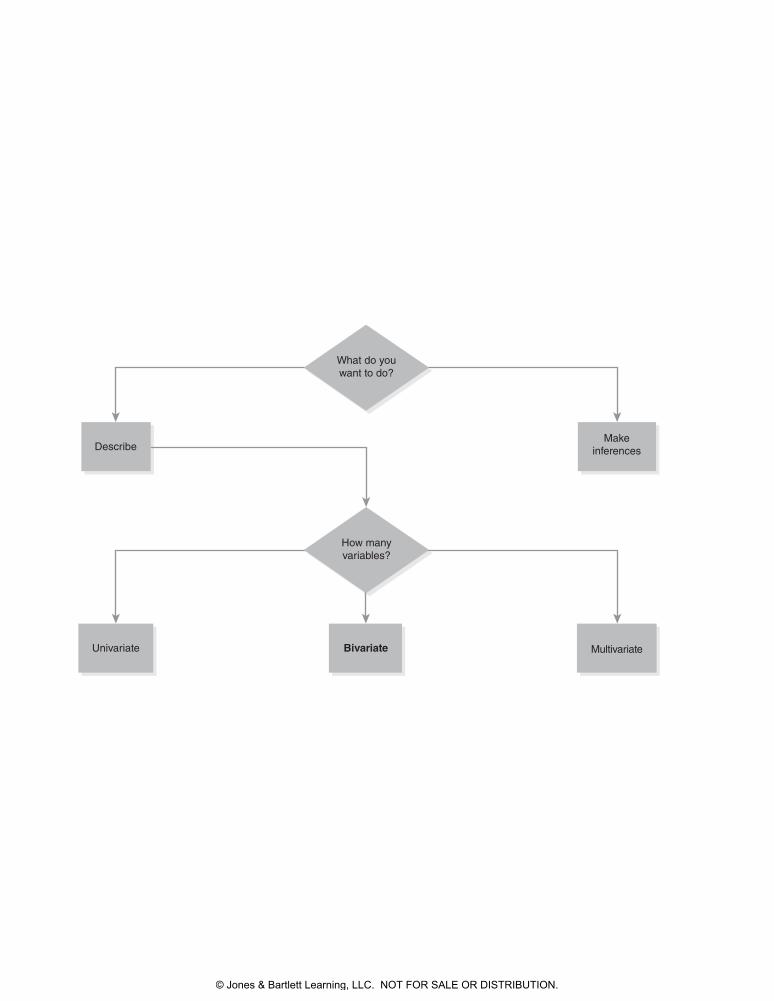
What do you want to do? Describe Make inferences How many variables? Univariate Multivariate Bivariate © Jones & Bartlett Learning, LLC. NOT FOR SALE OR DISTRIBUTION.
Transcript of © Jones & Bartlett Learning, LLC NOT FOR SALE OR ...
© Jones & Bartlett Learning, LLCNOT FOR SALE OR DISTRIBUTION
© Jones & Bartlett Learning, LLCNOT FOR SALE OR DISTRIBUTION
© Jones & Bartlett Learning, LLCNOT FOR SALE OR DISTRIBUTION
© Jones & Bartlett Learning, LLCNOT FOR SALE OR DISTRIBUTION
© Jones & Bartlett Learning, LLCNOT FOR SALE OR DISTRIBUTION
© Jones & Bartlett Learning, LLCNOT FOR SALE OR DISTRIBUTION
© Jones & Bartlett Learning, LLCNOT FOR SALE OR DISTRIBUTION
© Jones & Bartlett Learning, LLCNOT FOR SALE OR DISTRIBUTION
© Jones & Bartlett Learning, LLCNOT FOR SALE OR DISTRIBUTION
© Jones & Bartlett Learning, LLCNOT FOR SALE OR DISTRIBUTION
© Jones & Bartlett Learning, LLCNOT FOR SALE OR DISTRIBUTION
© Jones & Bartlett Learning, LLCNOT FOR SALE OR DISTRIBUTION
© Jones & Bartlett Learning, LLCNOT FOR SALE OR DISTRIBUTION
© Jones & Bartlett Learning, LLCNOT FOR SALE OR DISTRIBUTION
© Jones & Bartlett Learning, LLCNOT FOR SALE OR DISTRIBUTION
© Jones & Bartlett Learning, LLCNOT FOR SALE OR DISTRIBUTION
© Jones & Bartlett Learning, LLCNOT FOR SALE OR DISTRIBUTION
© Jones & Bartlett Learning, LLCNOT FOR SALE OR DISTRIBUTION
© Jones & Bartlett Learning, LLCNOT FOR SALE OR DISTRIBUTION
© Jones & Bartlett Learning, LLCNOT FOR SALE OR DISTRIBUTION
What do youwant to do?
DescribeMake
inferences
How manyvariables?
Univariate MultivariateBivariate
© Jones & Bartlett Learning, LLC. NOT FOR SALE OR DISTRIBUTION.

© Jones & Bartlett Learning, LLCNOT FOR SALE OR DISTRIBUTION
© Jones & Bartlett Learning, LLCNOT FOR SALE OR DISTRIBUTION
© Jones & Bartlett Learning, LLCNOT FOR SALE OR DISTRIBUTION
© Jones & Bartlett Learning, LLCNOT FOR SALE OR DISTRIBUTION
© Jones & Bartlett Learning, LLCNOT FOR SALE OR DISTRIBUTION
© Jones & Bartlett Learning, LLCNOT FOR SALE OR DISTRIBUTION
© Jones & Bartlett Learning, LLCNOT FOR SALE OR DISTRIBUTION
© Jones & Bartlett Learning, LLCNOT FOR SALE OR DISTRIBUTION
© Jones & Bartlett Learning, LLCNOT FOR SALE OR DISTRIBUTION
© Jones & Bartlett Learning, LLCNOT FOR SALE OR DISTRIBUTION
© Jones & Bartlett Learning, LLCNOT FOR SALE OR DISTRIBUTION
© Jones & Bartlett Learning, LLCNOT FOR SALE OR DISTRIBUTION
© Jones & Bartlett Learning, LLCNOT FOR SALE OR DISTRIBUTION
© Jones & Bartlett Learning, LLCNOT FOR SALE OR DISTRIBUTION
© Jones & Bartlett Learning, LLCNOT FOR SALE OR DISTRIBUTION
© Jones & Bartlett Learning, LLCNOT FOR SALE OR DISTRIBUTION
© Jones & Bartlett Learning, LLCNOT FOR SALE OR DISTRIBUTION
© Jones & Bartlett Learning, LLCNOT FOR SALE OR DISTRIBUTION
© Jones & Bartlett Learning, LLCNOT FOR SALE OR DISTRIBUTION
© Jones & Bartlett Learning, LLCNOT FOR SALE OR DISTRIBUTION
© Larry Washburn/Getty Images
CHAPTER 7
Introduction to Bivariate Descriptive Statistics
LEARNING OBJECTIVES
SECRETS FOR SUCCESS
1. Read the chapter carefully, making sure to work through the examples to ensure you understand them.
2. Answer the following questions about the examples:a. In Table 7-3, which crime had the largest overall percentage of respondents indicate
they were a victim of that crime?b. Explain why Table 7-5 might be confusing to a reader and what you might be able to do
to make the message you want to convey clearer.c. What are the marginals for Table 7-5?
3. Complete the following exercises. For the variables sex (male, female) and victim (yes, no):a. Fill in the information in the blanks to properly format the table.
by
1 2
2 20 37 57
1 27 48 75
47 85 132
b. Is this a nominal or an ordinal table? Why?
■ Describe the purpose of a bivariate table. ■ Explain how to construct a bivariate table. ■ Describe how to determine the cell number of a bivariate table. ■ Properly fill in a blank bivariate table with correct elements.
(continues)© Jones & Bartlett Learning, LLC. NOT FOR SALE OR DISTRIBUTION.

© Jones & Bartlett Learning, LLCNOT FOR SALE OR DISTRIBUTION
© Jones & Bartlett Learning, LLCNOT FOR SALE OR DISTRIBUTION
© Jones & Bartlett Learning, LLCNOT FOR SALE OR DISTRIBUTION
© Jones & Bartlett Learning, LLCNOT FOR SALE OR DISTRIBUTION
© Jones & Bartlett Learning, LLCNOT FOR SALE OR DISTRIBUTION
© Jones & Bartlett Learning, LLCNOT FOR SALE OR DISTRIBUTION
© Jones & Bartlett Learning, LLCNOT FOR SALE OR DISTRIBUTION
© Jones & Bartlett Learning, LLCNOT FOR SALE OR DISTRIBUTION
© Jones & Bartlett Learning, LLCNOT FOR SALE OR DISTRIBUTION
© Jones & Bartlett Learning, LLCNOT FOR SALE OR DISTRIBUTION
© Jones & Bartlett Learning, LLCNOT FOR SALE OR DISTRIBUTION
© Jones & Bartlett Learning, LLCNOT FOR SALE OR DISTRIBUTION
© Jones & Bartlett Learning, LLCNOT FOR SALE OR DISTRIBUTION
© Jones & Bartlett Learning, LLCNOT FOR SALE OR DISTRIBUTION
© Jones & Bartlett Learning, LLCNOT FOR SALE OR DISTRIBUTION
© Jones & Bartlett Learning, LLCNOT FOR SALE OR DISTRIBUTION
© Jones & Bartlett Learning, LLCNOT FOR SALE OR DISTRIBUTION
© Jones & Bartlett Learning, LLCNOT FOR SALE OR DISTRIBUTION
© Jones & Bartlett Learning, LLCNOT FOR SALE OR DISTRIBUTION
© Jones & Bartlett Learning, LLCNOT FOR SALE OR DISTRIBUTION
In Chapter 3, “Understanding Data Through Organization,” we introduced frequency tables as a method of examining the characteristics of a particular variable. It is possible to use those frequency tables to examine the relationship between two variables. As an example, consider the two variables sex and type of victimization. The combination tables from SPSS for each variable are shown in TABLE 7-1. The univariate statistics of each of these variables can be determined from these frequency tables. They show that there are more than double the number of female respondents as male respondents and that the most frequent victim-ization was for burglary, closely followed by vandalism and rape. The table for victimization also contains 229 people who indicated on a previous question that they had been victim-ized but who did not respond as to the actual crime in this question.
4. Read the chapter again. Make sure to do any “Stop! Do This” exercises you have not already successfully completed.
5. As you read the chapter, write down questions and things you do not understand to go over in class.
SECRETS FOR SUCCESS (continued )
TABLE 7-1 Combination Tables for Sex and Victimization
Sex of respondent
Value Label Value Frequency Percent Valid PercentCumulative
Percent
Male 1 99 28.5 29.1 29.1
Female 2 241 69.5 70.9 100.0
Missing 7 2.0
Total 347 100.0 100.0
Valid cases, 340; missing cases, 7.
Have you been a victim of any of these crimes in the last 6 months?
Value Label Value Frequency Percent Valid PercentCumulative
Percent
No response 0 7 2.0 5.9 5.9
Burglary 1 30 8.6 25.4 31.4
Vandalism 2 28 8.1 23.7 55.1
Car theft 3 14 4.0 11.9 66.9
Robbery 4 9 2.6 7.6 74.6
126 Chapter 7 Introduction to Bivariate Descriptive Statistics
© Jones & Bartlett Learning, LLC. NOT FOR SALE OR DISTRIBUTION.

© Jones & Bartlett Learning, LLCNOT FOR SALE OR DISTRIBUTION
© Jones & Bartlett Learning, LLCNOT FOR SALE OR DISTRIBUTION
© Jones & Bartlett Learning, LLCNOT FOR SALE OR DISTRIBUTION
© Jones & Bartlett Learning, LLCNOT FOR SALE OR DISTRIBUTION
© Jones & Bartlett Learning, LLCNOT FOR SALE OR DISTRIBUTION
© Jones & Bartlett Learning, LLCNOT FOR SALE OR DISTRIBUTION
© Jones & Bartlett Learning, LLCNOT FOR SALE OR DISTRIBUTION
© Jones & Bartlett Learning, LLCNOT FOR SALE OR DISTRIBUTION
© Jones & Bartlett Learning, LLCNOT FOR SALE OR DISTRIBUTION
© Jones & Bartlett Learning, LLCNOT FOR SALE OR DISTRIBUTION
© Jones & Bartlett Learning, LLCNOT FOR SALE OR DISTRIBUTION
© Jones & Bartlett Learning, LLCNOT FOR SALE OR DISTRIBUTION
© Jones & Bartlett Learning, LLCNOT FOR SALE OR DISTRIBUTION
© Jones & Bartlett Learning, LLCNOT FOR SALE OR DISTRIBUTION
© Jones & Bartlett Learning, LLCNOT FOR SALE OR DISTRIBUTION
© Jones & Bartlett Learning, LLCNOT FOR SALE OR DISTRIBUTION
© Jones & Bartlett Learning, LLCNOT FOR SALE OR DISTRIBUTION
© Jones & Bartlett Learning, LLCNOT FOR SALE OR DISTRIBUTION
© Jones & Bartlett Learning, LLCNOT FOR SALE OR DISTRIBUTION
© Jones & Bartlett Learning, LLCNOT FOR SALE OR DISTRIBUTION
It is difficult, however, to make any determinations about the possible sex of victims from these tables. For instance, it is impossible to determine from these tables how many males and how many females were victims of burglary. However, with some additional work and analyses, the tables can be arranged by the sex of the respondent. This allows statements to be made about male and female victims. With the data provided in TABLE 7-2, it can be shown that females experienced a higher number and percentage of vandalism, car theft, assault, and rape and that males had a higher percentage of burglaries, robberies, and other victimizations (although there were still more females in each of these categories except burglary, which had the same number of males and females, and no response). This is a somewhat complicated process, however, and requires looking back and forth between tables. It would be much easier if we could make more direct, or side-by-side, comparisons of the variables. A bivariate table does just that.
Value Label Value Frequency Percent Valid PercentCumulative
Percent
Assault 5 3 0.9 2.5 77.1
Rape 6 22 6.3 18.6 95.6
Other 7 5 1.4 4.2 100.0
Missing 229 66.0
Total 347 100.0 100.0
Valid cases, 118; missing cases, 229.
TABLE 7-2 Data for Male and Female Victims of Crime
Type of Crime
Male Victim Female Victim
Frequency Percent Frequency Percent
No response 1 2.9 4 5.1
Burglary 15 42.9 15 19.0
Vandalism 5 14.3 21 26.6
Car theft 3 8.6 11 13.9
Robbery 3 8.6 6 7.6
Assault 0 0 3 3.8
Rape 5 14.3 17 21.5
Other 3 8.6 2 2.5
127Introduction to Bivariate Descriptive Statistics
© Jones & Bartlett Learning, LLC. NOT FOR SALE OR DISTRIBUTION.
© Jones & Bartlett Learning, LLCNOT FOR SALE OR DISTRIBUTION
© Jones & Bartlett Learning, LLCNOT FOR SALE OR DISTRIBUTION
© Jones & Bartlett Learning, LLCNOT FOR SALE OR DISTRIBUTION
© Jones & Bartlett Learning, LLCNOT FOR SALE OR DISTRIBUTION
© Jones & Bartlett Learning, LLCNOT FOR SALE OR DISTRIBUTION
© Jones & Bartlett Learning, LLCNOT FOR SALE OR DISTRIBUTION
© Jones & Bartlett Learning, LLCNOT FOR SALE OR DISTRIBUTION
© Jones & Bartlett Learning, LLCNOT FOR SALE OR DISTRIBUTION
© Jones & Bartlett Learning, LLCNOT FOR SALE OR DISTRIBUTION
© Jones & Bartlett Learning, LLCNOT FOR SALE OR DISTRIBUTION
© Jones & Bartlett Learning, LLCNOT FOR SALE OR DISTRIBUTION
© Jones & Bartlett Learning, LLCNOT FOR SALE OR DISTRIBUTION
© Jones & Bartlett Learning, LLCNOT FOR SALE OR DISTRIBUTION
© Jones & Bartlett Learning, LLCNOT FOR SALE OR DISTRIBUTION
© Jones & Bartlett Learning, LLCNOT FOR SALE OR DISTRIBUTION
© Jones & Bartlett Learning, LLCNOT FOR SALE OR DISTRIBUTION
© Jones & Bartlett Learning, LLCNOT FOR SALE OR DISTRIBUTION
© Jones & Bartlett Learning, LLCNOT FOR SALE OR DISTRIBUTION
© Jones & Bartlett Learning, LLCNOT FOR SALE OR DISTRIBUTION
© Jones & Bartlett Learning, LLCNOT FOR SALE OR DISTRIBUTION
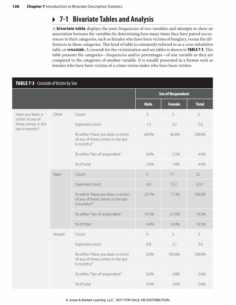
▸ 7-1 Bivariate Tables and AnalysisA bivariate table displays the joint frequencies of two variables and attempts to show an association between the variables by determining how many times they have paired occur-rences in their categories, such as females who have been victims of burglary, versus the dif-ferences in those categories. This kind of table is commonly referred to as a cross- tabulation table, or crosstab. A crosstab for the victimization and sex tables is shown in TABLE 7-3. This table presents the categories—frequencies and/or percentages—of one variable as they are compared to the categories of another variable. It is usually presented in a format such as females who have been victims of a crime versus males who have been victims.
TABLE 7-3 Crosstab of Victim by Sex
Sex of Respondent
Male Female Total
Have you been a victim of any of these crimes in the last 6 months?
Other Count 3 2 5
Expected count 1.5 3.5 5.0
% within “Have you been a victim of any of these crimes in the last 6 months?”
60.0% 40.0% 100.0%
% within “Sex of respondent” 8.6% 2.5% 4.4%
% of total 2.6% 1.8% 4.4%
Rape Count 5 17 22
Expected count 6.8 15.2 22.0
% within “Have you been a victim of any of these crimes in the last 6 months?”
22.7% 77.3% 100.0%
% within “Sex of respondent” 14.3% 21.5% 19.3%
% of total 4.4% 14.9% 19.3%
Assault Count 0 3 3
Expected count 0.9 2.1 3.0
% within “Have you been a victim of any of these crimes in the last 6 months?”
0.0% 100.0% 100.0%
% within “Sex of respondent” 0.0% 3.8% 2.6%
% of total 0.0% 2.6% 2.6%
128 Chapter 7 Introduction to Bivariate Descriptive Statistics
© Jones & Bartlett Learning, LLC. NOT FOR SALE OR DISTRIBUTION.

© Jones & Bartlett Learning, LLCNOT FOR SALE OR DISTRIBUTION
© Jones & Bartlett Learning, LLCNOT FOR SALE OR DISTRIBUTION
© Jones & Bartlett Learning, LLCNOT FOR SALE OR DISTRIBUTION
© Jones & Bartlett Learning, LLCNOT FOR SALE OR DISTRIBUTION
© Jones & Bartlett Learning, LLCNOT FOR SALE OR DISTRIBUTION
© Jones & Bartlett Learning, LLCNOT FOR SALE OR DISTRIBUTION
© Jones & Bartlett Learning, LLCNOT FOR SALE OR DISTRIBUTION
© Jones & Bartlett Learning, LLCNOT FOR SALE OR DISTRIBUTION
© Jones & Bartlett Learning, LLCNOT FOR SALE OR DISTRIBUTION
© Jones & Bartlett Learning, LLCNOT FOR SALE OR DISTRIBUTION
© Jones & Bartlett Learning, LLCNOT FOR SALE OR DISTRIBUTION
© Jones & Bartlett Learning, LLCNOT FOR SALE OR DISTRIBUTION
© Jones & Bartlett Learning, LLCNOT FOR SALE OR DISTRIBUTION
© Jones & Bartlett Learning, LLCNOT FOR SALE OR DISTRIBUTION
© Jones & Bartlett Learning, LLCNOT FOR SALE OR DISTRIBUTION
© Jones & Bartlett Learning, LLCNOT FOR SALE OR DISTRIBUTION
© Jones & Bartlett Learning, LLCNOT FOR SALE OR DISTRIBUTION
© Jones & Bartlett Learning, LLCNOT FOR SALE OR DISTRIBUTION
© Jones & Bartlett Learning, LLCNOT FOR SALE OR DISTRIBUTION
© Jones & Bartlett Learning, LLCNOT FOR SALE OR DISTRIBUTION
Sex of Respondent
Male Female Total
Robbery Count 3 6 9
Expected count 2.8 6.2 9.0
% within “Have you been a victim of any of these crimes in the last 6 months?”
33.3% 66.7% 100.0%
% within “Sex of respondent” 8.6% 7.6% 7.9%
% of total 2.6% 5.3% 7.9%
Car theft Count 3 11 14
Expected count 4.3 9.7 14.0
% within “Have you been a victim of any of these crimes in the last 6 months?”
21.4% 78.6% 100.0%
% within “Sex of respondent” 8.6% 13.9% 12.3%
% of total 2.6% 9.6% 12.3%
Vandalism Count 5 21 26
Expected count 8.0 18.0 26.0
% within “Have you been a victim of any of these crimes in the last 6 months?”
19.2% 80.8% 100.0%
% within “Sex of respondent” 14.3% 26.6% 22.8%
% of total 4.4% 18.4% 22.8%
Burglary Count 15 15 30
Expected count 9.2 20.8 30.0
% within “Have you been a victim of any of these crimes in the last 6 months?”
50.0% 50.0% 100.0%
% within “Sex of respondent” 42.9% 19.0% 26.3%
% of total 13.2% 13.2% 26.3%
(continues)
7-1 Bivariate Tables and Analysis 129
© Jones & Bartlett Learning, LLC. NOT FOR SALE OR DISTRIBUTION.

© Jones & Bartlett Learning, LLCNOT FOR SALE OR DISTRIBUTION
© Jones & Bartlett Learning, LLCNOT FOR SALE OR DISTRIBUTION
© Jones & Bartlett Learning, LLCNOT FOR SALE OR DISTRIBUTION
© Jones & Bartlett Learning, LLCNOT FOR SALE OR DISTRIBUTION
© Jones & Bartlett Learning, LLCNOT FOR SALE OR DISTRIBUTION
© Jones & Bartlett Learning, LLCNOT FOR SALE OR DISTRIBUTION
© Jones & Bartlett Learning, LLCNOT FOR SALE OR DISTRIBUTION
© Jones & Bartlett Learning, LLCNOT FOR SALE OR DISTRIBUTION
© Jones & Bartlett Learning, LLCNOT FOR SALE OR DISTRIBUTION
© Jones & Bartlett Learning, LLCNOT FOR SALE OR DISTRIBUTION
© Jones & Bartlett Learning, LLCNOT FOR SALE OR DISTRIBUTION
© Jones & Bartlett Learning, LLCNOT FOR SALE OR DISTRIBUTION
© Jones & Bartlett Learning, LLCNOT FOR SALE OR DISTRIBUTION
© Jones & Bartlett Learning, LLCNOT FOR SALE OR DISTRIBUTION
© Jones & Bartlett Learning, LLCNOT FOR SALE OR DISTRIBUTION
© Jones & Bartlett Learning, LLCNOT FOR SALE OR DISTRIBUTION
© Jones & Bartlett Learning, LLCNOT FOR SALE OR DISTRIBUTION
© Jones & Bartlett Learning, LLCNOT FOR SALE OR DISTRIBUTION
© Jones & Bartlett Learning, LLCNOT FOR SALE OR DISTRIBUTION
© Jones & Bartlett Learning, LLCNOT FOR SALE OR DISTRIBUTION
TABLE 7-3 Crosstab of Victim by Sex (continued )
Sex of Respondent
Male Female Total
No response Count 1 4 5
Expected count 1.5 3.5 5.0
% within “Have you been a victim of any of these crimes in the last 6 months?”
20.0% 80.0% 100.0%
% within “Sex of respondent” 2.9% 5.1% 4.4%
% of total 0.9% 3.5% 4.4%
Total Count 35 79 114
Expected count 35.0 79.0 114.0
% within “Have you been a victim of any of these crimes in the last 6 months?”
30.7% 69.3% 100.0%
% within “Sex of respondent” 100.0% 100.0% 100.0%
% of total 30.7% 69.3% 100.0%
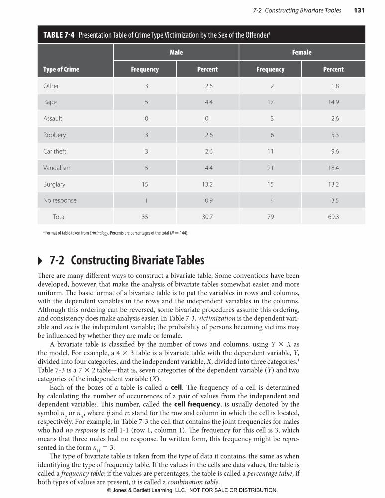
Statistical Tables Versus Presentation TablesTables may be broken into two general types: statistical tables and presentation tables. Statistical tables are those represented by the output from statistical programs such as SPSS and are used in this text. Presentation tables are those found in journals and books. These tables are generally made by taking the statistical tables and formatting them to fit (1) a particular editorial style, such as Turabian or APA; (2) the format required by a particular publication; or (3) the aesthetic notions of the author—that is, what he or she thinks looks best.
It is important to be able to understand and interpret both types of tables. Much of what you will see as students will be presentation tables in journal articles. Most such tables are fairly easy to understand because the reason they are created the way they are is to make them easy to read. What is probably more important, however, is the ability to read statistical tables. If you cannot read statistical tables, it is not possible to analyze the data or to convert the statistical tables to presentation tables. For this reason, in this text we focus on statistical tables. The tables contained here are direct output from SPSS. They will allow you to begin to understand statistical output, to be able to analyze that output, and to be able to put that analysis in writing. To show the difference between statistical tables and presentation tables, the information in Table 7-3 is shown as a presentation table in TABLE 7-4.
Some tables in this text will be shown as both statistical tables and presentation tables to show the differences and similarities. The focus of the tables, however, is on statistical tables and analysis.
130 Chapter 7 Introduction to Bivariate Descriptive Statistics
© Jones & Bartlett Learning, LLC. NOT FOR SALE OR DISTRIBUTION.
© Jones & Bartlett Learning, LLCNOT FOR SALE OR DISTRIBUTION
© Jones & Bartlett Learning, LLCNOT FOR SALE OR DISTRIBUTION
© Jones & Bartlett Learning, LLCNOT FOR SALE OR DISTRIBUTION
© Jones & Bartlett Learning, LLCNOT FOR SALE OR DISTRIBUTION
© Jones & Bartlett Learning, LLCNOT FOR SALE OR DISTRIBUTION
© Jones & Bartlett Learning, LLCNOT FOR SALE OR DISTRIBUTION
© Jones & Bartlett Learning, LLCNOT FOR SALE OR DISTRIBUTION
© Jones & Bartlett Learning, LLCNOT FOR SALE OR DISTRIBUTION
© Jones & Bartlett Learning, LLCNOT FOR SALE OR DISTRIBUTION
© Jones & Bartlett Learning, LLCNOT FOR SALE OR DISTRIBUTION
© Jones & Bartlett Learning, LLCNOT FOR SALE OR DISTRIBUTION
© Jones & Bartlett Learning, LLCNOT FOR SALE OR DISTRIBUTION
© Jones & Bartlett Learning, LLCNOT FOR SALE OR DISTRIBUTION
© Jones & Bartlett Learning, LLCNOT FOR SALE OR DISTRIBUTION
© Jones & Bartlett Learning, LLCNOT FOR SALE OR DISTRIBUTION
© Jones & Bartlett Learning, LLCNOT FOR SALE OR DISTRIBUTION
© Jones & Bartlett Learning, LLCNOT FOR SALE OR DISTRIBUTION
© Jones & Bartlett Learning, LLCNOT FOR SALE OR DISTRIBUTION
© Jones & Bartlett Learning, LLCNOT FOR SALE OR DISTRIBUTION
© Jones & Bartlett Learning, LLCNOT FOR SALE OR DISTRIBUTION
▸ 7-2 Constructing Bivariate TablesThere are many different ways to construct a bivariate table. Some conventions have been developed, however, that make the analysis of bivariate tables somewhat easier and more uniform. The basic format of a bivariate table is to put the variables in rows and columns, with the dependent variables in the rows and the independent variables in the columns. Although this ordering can be reversed, some bivariate procedures assume this ordering, and consistency does make analysis easier. In Table 7-3, victimization is the dependent vari-able and sex is the independent variable; the probability of persons becoming victims may be influenced by whether they are male or female.
A bivariate table is classified by the number of rows and columns, using Y 3 X as the model. For example, a 4 3 3 table is a bivariate table with the dependent variable, Y, divided into four categories, and the independent variable, X, divided into three categories.1 Table 7-3 is a 7 3 2 table—that is, seven categories of the dependent variable (Y) and two categories of the independent variable (X).
Each of the boxes of a table is called a cell. The frequency of a cell is determined by calculating the number of occurrences of a pair of values from the independent and dependent variables. This number, called the cell frequency, is usually denoted by the symbol nij or nrc, where ij and rc stand for the row and column in which the cell is located, respectively. For example, in Table 7-3 the cell that contains the joint frequencies for males who had no response is cell 1-1 (row 1, column 1). The frequency for this cell is 3, which means that three males had no response. In written form, this frequency might be repre-sented in the form n11 5 3.
The type of bivariate table is taken from the type of data it contains, the same as when identifying the type of frequency table. If the values in the cells are data values, the table is called a frequency table; if the values are percentages, the table is called a percentage table; if both types of values are present, it is called a combination table.
TABLE 7-4 Presentation Table of Crime Type Victimization by the Sex of the Offendera
Type of Crime
Male Female
Frequency Percent Frequency Percent
Other 3 2.6 2 1.8
Rape 5 4.4 17 14.9
Assault 0 0 3 2.6
Robbery 3 2.6 6 5.3
Car theft 3 2.6 11 9.6
Vandalism 5 4.4 21 18.4
Burglary 15 13.2 15 13.2
No response 1 0.9 4 3.5
Total 35 30.7 79 69.3
a Format of table taken from Criminology. Percents are percentages of the total (N 5 144).
7-2 Constructing Bivariate Tables 131
© Jones & Bartlett Learning, LLC. NOT FOR SALE OR DISTRIBUTION.
© Jones & Bartlett Learning, LLCNOT FOR SALE OR DISTRIBUTION
© Jones & Bartlett Learning, LLCNOT FOR SALE OR DISTRIBUTION
© Jones & Bartlett Learning, LLCNOT FOR SALE OR DISTRIBUTION
© Jones & Bartlett Learning, LLCNOT FOR SALE OR DISTRIBUTION
© Jones & Bartlett Learning, LLCNOT FOR SALE OR DISTRIBUTION
© Jones & Bartlett Learning, LLCNOT FOR SALE OR DISTRIBUTION
© Jones & Bartlett Learning, LLCNOT FOR SALE OR DISTRIBUTION
© Jones & Bartlett Learning, LLCNOT FOR SALE OR DISTRIBUTION
© Jones & Bartlett Learning, LLCNOT FOR SALE OR DISTRIBUTION
© Jones & Bartlett Learning, LLCNOT FOR SALE OR DISTRIBUTION
© Jones & Bartlett Learning, LLCNOT FOR SALE OR DISTRIBUTION
© Jones & Bartlett Learning, LLCNOT FOR SALE OR DISTRIBUTION
© Jones & Bartlett Learning, LLCNOT FOR SALE OR DISTRIBUTION
© Jones & Bartlett Learning, LLCNOT FOR SALE OR DISTRIBUTION
© Jones & Bartlett Learning, LLCNOT FOR SALE OR DISTRIBUTION
© Jones & Bartlett Learning, LLCNOT FOR SALE OR DISTRIBUTION
© Jones & Bartlett Learning, LLCNOT FOR SALE OR DISTRIBUTION
© Jones & Bartlett Learning, LLCNOT FOR SALE OR DISTRIBUTION
© Jones & Bartlett Learning, LLCNOT FOR SALE OR DISTRIBUTION
© Jones & Bartlett Learning, LLCNOT FOR SALE OR DISTRIBUTION
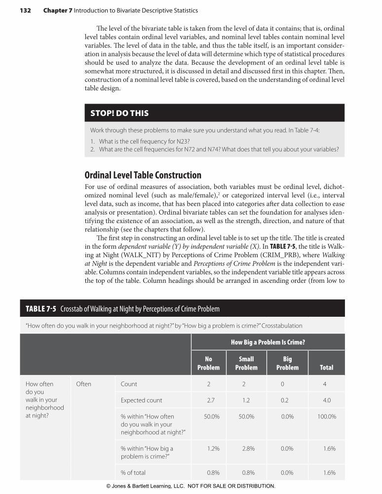
The level of the bivariate table is taken from the level of data it contains; that is, ordinal level tables contain ordinal level variables, and nominal level tables contain nominal level variables. The level of data in the table, and thus the table itself, is an important consider-ation in analysis because the level of data will determine which type of statistical procedures should be used to analyze the data. Because the development of an ordinal level table is somewhat more structured, it is discussed in detail and discussed first in this chapter. Then, construction of a nominal level table is covered, based on the understanding of ordinal level table design.
STOP! DO THIS
Work through these problems to make sure you understand what you read. In Table 7-4:
1. What is the cell frequency for N23?2. What are the cell frequencies for N72 and N74? What does that tell you about your variables?
Ordinal Level Table ConstructionFor use of ordinal measures of association, both variables must be ordinal level, dichot-omized nominal level (such as male/female),2 or categorized interval level (i.e., interval level data, such as income, that has been placed into categories after data collection to ease analysis or presentation). Ordinal bivariate tables can set the foundation for analyses iden-tifying the existence of an association, as well as the strength, direction, and nature of that relationship (see the chapters that follow).
The first step in constructing an ordinal level table is to set up the title. The title is created in the form dependent variable (Y) by independent variable (X). In TABLE 7-5, the title is Walk-ing at Night (WALK_NIT) by Perceptions of Crime Problem (CRIM_PRB), where Walking at Night is the dependent variable and Perceptions of Crime Problem is the independent vari-able. Columns contain independent variables, so the independent variable title appears across the top of the table. Column headings should be arranged in ascending order (from low to
TABLE 7-5 Crosstab of Walking at Night by Perceptions of Crime Problem
“How often do you walk in your neighborhood at night?” by “How big a problem is crime?” Crosstabulation
How Big a Problem Is Crime?
No Problem
Small Problem
Big Problem Total
How often do you walk in your neighborhood at night?
Often Count 2 2 0 4
Expected count 2.7 1.2 0.2 4.0
% within “How often do you walk in your neighborhood at night?”
50.0% 50.0% 0.0% 100.0%
% within “How big a problem is crime?”
1.2% 2.8% 0.0% 1.6%
% of total 0.8% 0.8% 0.0% 1.6%
132 Chapter 7 Introduction to Bivariate Descriptive Statistics
© Jones & Bartlett Learning, LLC. NOT FOR SALE OR DISTRIBUTION.

© Jones & Bartlett Learning, LLCNOT FOR SALE OR DISTRIBUTION
© Jones & Bartlett Learning, LLCNOT FOR SALE OR DISTRIBUTION
© Jones & Bartlett Learning, LLCNOT FOR SALE OR DISTRIBUTION
© Jones & Bartlett Learning, LLCNOT FOR SALE OR DISTRIBUTION
© Jones & Bartlett Learning, LLCNOT FOR SALE OR DISTRIBUTION
© Jones & Bartlett Learning, LLCNOT FOR SALE OR DISTRIBUTION
© Jones & Bartlett Learning, LLCNOT FOR SALE OR DISTRIBUTION
© Jones & Bartlett Learning, LLCNOT FOR SALE OR DISTRIBUTION
© Jones & Bartlett Learning, LLCNOT FOR SALE OR DISTRIBUTION
© Jones & Bartlett Learning, LLCNOT FOR SALE OR DISTRIBUTION
© Jones & Bartlett Learning, LLCNOT FOR SALE OR DISTRIBUTION
© Jones & Bartlett Learning, LLCNOT FOR SALE OR DISTRIBUTION
© Jones & Bartlett Learning, LLCNOT FOR SALE OR DISTRIBUTION
© Jones & Bartlett Learning, LLCNOT FOR SALE OR DISTRIBUTION
© Jones & Bartlett Learning, LLCNOT FOR SALE OR DISTRIBUTION
© Jones & Bartlett Learning, LLCNOT FOR SALE OR DISTRIBUTION
© Jones & Bartlett Learning, LLCNOT FOR SALE OR DISTRIBUTION
© Jones & Bartlett Learning, LLCNOT FOR SALE OR DISTRIBUTION
© Jones & Bartlett Learning, LLCNOT FOR SALE OR DISTRIBUTION
© Jones & Bartlett Learning, LLCNOT FOR SALE OR DISTRIBUTION
How Big a Problem Is Crime?
No Problem
Small Problem
Big Problem Total
Occasionally Count 20 13 3 36
Expected count 23.9 10.4 1.7 36.0
% within “How often do you walk in your neighborhood at night?”
55.6% 36.1% 8.3% 100.0%
% within “How big a problem is crime?”
12.1% 18.1% 25.0% 14.5%
% of total 8.0% 5.2% 1.2% 14.5%
Never Count 143 57 9 209
Expected count 138.5 60.4 10.1 209.0
% within “How often do you walk in your neighborhood at night?”
68.4% 27.3% 4.3% 100.0%
% within “How big a problem is crime?”
86.7% 79.2% 75.0% 83.9%
% of total 57.4% 22.9% 3.6% 83.9%
Total Count 165 72 12 249
Expected count 165.0 72.0 12.0 249.0
% within “How often do you walk in your neighborhood at night?”
66.3% 28.9% 4.8% 100.0%
% within “How big a problem is crime?”
100.0% 100.0% 100.0% 100.0%
% of total 66.3% 28.9% 4.8% 100.0%
high) as you move from left to right across the table. In the example shown in Table 7-5, the categories of CRIM_PRB move from No Problem (category 1) to Big Problem (category 3) as you move across the top of the table. Rows contain the dependent variables, so the dependent variable title appears to the left of the table. Row headings should be arranged in descending order (from high to low) as you move from the top to the bottom of the table. In Table 7-5, the rows for WALK_NIT move from Often (category 3) to Never (category 1) as you move from top to bottom. Arranging the dependent variable so it moves from high values at the top of the table to low values at the bottom of the table will ensure the signs of analyses will be correct and the direction is visually attainable by how the values are arranged.
7-2 Constructing Bivariate Tables 133
© Jones & Bartlett Learning, LLC. NOT FOR SALE OR DISTRIBUTION.
© Jones & Bartlett Learning, LLCNOT FOR SALE OR DISTRIBUTION
© Jones & Bartlett Learning, LLCNOT FOR SALE OR DISTRIBUTION
© Jones & Bartlett Learning, LLCNOT FOR SALE OR DISTRIBUTION
© Jones & Bartlett Learning, LLCNOT FOR SALE OR DISTRIBUTION
© Jones & Bartlett Learning, LLCNOT FOR SALE OR DISTRIBUTION
© Jones & Bartlett Learning, LLCNOT FOR SALE OR DISTRIBUTION
© Jones & Bartlett Learning, LLCNOT FOR SALE OR DISTRIBUTION
© Jones & Bartlett Learning, LLCNOT FOR SALE OR DISTRIBUTION
© Jones & Bartlett Learning, LLCNOT FOR SALE OR DISTRIBUTION
© Jones & Bartlett Learning, LLCNOT FOR SALE OR DISTRIBUTION
© Jones & Bartlett Learning, LLCNOT FOR SALE OR DISTRIBUTION
© Jones & Bartlett Learning, LLCNOT FOR SALE OR DISTRIBUTION
© Jones & Bartlett Learning, LLCNOT FOR SALE OR DISTRIBUTION
© Jones & Bartlett Learning, LLCNOT FOR SALE OR DISTRIBUTION
© Jones & Bartlett Learning, LLCNOT FOR SALE OR DISTRIBUTION
© Jones & Bartlett Learning, LLCNOT FOR SALE OR DISTRIBUTION
© Jones & Bartlett Learning, LLCNOT FOR SALE OR DISTRIBUTION
© Jones & Bartlett Learning, LLCNOT FOR SALE OR DISTRIBUTION
© Jones & Bartlett Learning, LLCNOT FOR SALE OR DISTRIBUTION
© Jones & Bartlett Learning, LLCNOT FOR SALE OR DISTRIBUTION
In this case, there were no No Problem responses, so there were no category 1 responses to hash-mark. When these results are put in terms of a frequency, they would look like the top row in Table 7-5.
HOW DO YOU DO THAT?
Constructing a Bivariate Table in SPSS1. Open a data set.
a. Start SPSS.b. Click File, then Open, then Data.c. Select the file you want to open, then click Open.
2. Once the data is visible, click Analyze, then Descriptive Statistics, then Crosstabs.3. Select the variable you wish to include as your dependent variable, and click the ▶ next to
the Row(s) window.4. Select the variable you wish to include as your independent variable, and click the ▶ next to
the Column(s) window.5. For now, do not worry about the “Exact” and “Statistics” boxes at the bottom of the window.6. Click the Cells button, and then check any of the boxes for information you may want in your
crosstab. For a crosstab with full information, select “observed,” “expected,” “row,” “column,” and “total”; then click Continue.
7. Important: Click the Format button, and check the box marked “Descending.” If you do not do this, your table will not be formatted as discussed in this chapter.
An output window should appear containing a distribution similar in format to Table 7-3.
Ordering the variables and categories as described here is a convention, but one that is not always followed. Some statistical programs, including SPSS, do not automatically set the variables in the position described here, nor do they automatically order the categories as outlined in this chapter. Because of the need for flexibility when working with data, most programs allow a researcher to specify variable arrangements and category orders. When conducting research, then, it is important to ensure that a table is set up in the prescribed manner before conducting additional analyses; otherwise, the analyses described in this text will not work. It is not that you could not analyze the data, but rather that you would have to use different methods than those described here because the table would be back-ward to how the analysis is addressed in this text.
To fill out the table, place the proper numbers in each cell by counting how many times each pair occurs. The data that would be contained in the top row of Table 7-5 is shown next. For each of the two variables, the cell frequencies would be determined by taking each pair of scores and hash-marking them in the appropriate cell. Once all of the pairs of values have been determined, these hash marks could be converted to frequencies. In this example, two respondents stated that they often walked at night and that crime was a small problem in their neighborhood, and two people said that they often walked at night and that crime was a big problem in their neighborhood.
Respondent WALK_NIT CRIM_PRB
ABCD
Often (3)Often (3)Often (3)Often (3)
Small problem (2)Big problem (3)Big problem (3)Small problem (2)
134 Chapter 7 Introduction to Bivariate Descriptive Statistics
© Jones & Bartlett Learning, LLC. NOT FOR SALE OR DISTRIBUTION.
© Jones & Bartlett Learning, LLCNOT FOR SALE OR DISTRIBUTION
© Jones & Bartlett Learning, LLCNOT FOR SALE OR DISTRIBUTION
© Jones & Bartlett Learning, LLCNOT FOR SALE OR DISTRIBUTION
© Jones & Bartlett Learning, LLCNOT FOR SALE OR DISTRIBUTION
© Jones & Bartlett Learning, LLCNOT FOR SALE OR DISTRIBUTION
© Jones & Bartlett Learning, LLCNOT FOR SALE OR DISTRIBUTION
© Jones & Bartlett Learning, LLCNOT FOR SALE OR DISTRIBUTION
© Jones & Bartlett Learning, LLCNOT FOR SALE OR DISTRIBUTION
© Jones & Bartlett Learning, LLCNOT FOR SALE OR DISTRIBUTION
© Jones & Bartlett Learning, LLCNOT FOR SALE OR DISTRIBUTION
© Jones & Bartlett Learning, LLCNOT FOR SALE OR DISTRIBUTION
© Jones & Bartlett Learning, LLCNOT FOR SALE OR DISTRIBUTION
© Jones & Bartlett Learning, LLCNOT FOR SALE OR DISTRIBUTION
© Jones & Bartlett Learning, LLCNOT FOR SALE OR DISTRIBUTION
© Jones & Bartlett Learning, LLCNOT FOR SALE OR DISTRIBUTION
© Jones & Bartlett Learning, LLCNOT FOR SALE OR DISTRIBUTION
© Jones & Bartlett Learning, LLCNOT FOR SALE OR DISTRIBUTION
© Jones & Bartlett Learning, LLCNOT FOR SALE OR DISTRIBUTION
© Jones & Bartlett Learning, LLCNOT FOR SALE OR DISTRIBUTION
© Jones & Bartlett Learning, LLCNOT FOR SALE OR DISTRIBUTION
STOP! DO THIS
Work through these problems to make sure you understand what you read.
1. In which cell would respondent C fit in Table 7-5?2. Express that in terms of Nrc.
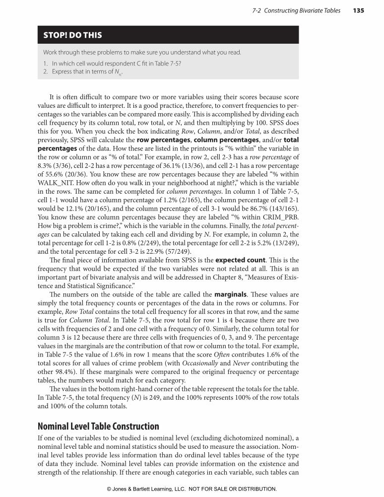
It is often difficult to compare two or more variables using their scores because score values are difficult to interpret. It is a good practice, therefore, to convert frequencies to per-centages so the variables can be compared more easily. This is accomplished by dividing each cell frequency by its column total, row total, or N, and then multiplying by 100. SPSS does this for you. When you check the box indicating Row, Column, and/or Total, as described previously, SPSS will calculate the row percentages, column percentages, and/or total percentages of the data. How these are listed in the printouts is “% within” the variable in the row or column or as “% of total.” For example, in row 2, cell 2-3 has a row percentage of 8.3% (3/36), cell 2-2 has a row percentage of 36.1% (13/36), and cell 2-1 has a row percentage of 55.6% (20/36). You know these are row percentages because they are labeled “% within WALK_NIT. How often do you walk in your neighborhood at night?,” which is the variable in the rows. The same can be completed for column percentages. In column 1 of Table 7-5, cell 1-1 would have a column percentage of 1.2% (2/165), the column percentage of cell 2-1 would be 12.1% (20/165), and the column percentage of cell 3-1 would be 86.7% (143/165). You know these are column percentages because they are labeled “% within CRIM_PRB. How big a problem is crime?,” which is the variable in the columns. Finally, the total percent-ages can be calculated by taking each cell and dividing by N. For example, in column 2, the total percentage for cell 1-2 is 0.8% (2/249), the total percentage for cell 2-2 is 5.2% (13/249), and the total percentage for cell 3-2 is 22.9% (57/249).
The final piece of information available from SPSS is the expected count. This is the frequency that would be expected if the two variables were not related at all. This is an important part of bivariate analysis and will be addressed in Chapter 8, “Measures of Exis-tence and Statistical Significance.”
The numbers on the outside of the table are called the marginals. These values are simply the total frequency counts or percentages of the data in the rows or columns. For example, Row Total contains the total cell frequency for all scores in that row, and the same is true for Column Total. In Table 7-5, the row total for row 1 is 4 because there are two cells with frequencies of 2 and one cell with a frequency of 0. Similarly, the column total for column 3 is 12 because there are three cells with frequencies of 0, 3, and 9. The percentage values in the marginals are the contribution of that row or column to the total. For example, in Table 7-5 the value of 1.6% in row 1 means that the score Often contributes 1.6% of the total scores for all values of crime problem (with Occasionally and Never contributing the other 98.4%). If these marginals were compared to the original frequency or percentage tables, the numbers would match for each category.
The values in the bottom right-hand corner of the table represent the totals for the table. In Table 7-5, the total frequency (N) is 249, and the 100% represents 100% of the row totals and 100% of the column totals.
Nominal Level Table ConstructionIf one of the variables to be studied is nominal level (excluding dichotomized nominal), a nominal level table and nominal statistics should be used to measure the association. Nom-inal level tables provide less information than do ordinal level tables because of the type of data they include. Nominal level tables can provide information on the existence and strength of the relationship. If there are enough categories in each variable, such tables can
7-2 Constructing Bivariate Tables 135
© Jones & Bartlett Learning, LLC. NOT FOR SALE OR DISTRIBUTION.
© Jones & Bartlett Learning, LLCNOT FOR SALE OR DISTRIBUTION
© Jones & Bartlett Learning, LLCNOT FOR SALE OR DISTRIBUTION
© Jones & Bartlett Learning, LLCNOT FOR SALE OR DISTRIBUTION
© Jones & Bartlett Learning, LLCNOT FOR SALE OR DISTRIBUTION
© Jones & Bartlett Learning, LLCNOT FOR SALE OR DISTRIBUTION
© Jones & Bartlett Learning, LLCNOT FOR SALE OR DISTRIBUTION
© Jones & Bartlett Learning, LLCNOT FOR SALE OR DISTRIBUTION
© Jones & Bartlett Learning, LLCNOT FOR SALE OR DISTRIBUTION
© Jones & Bartlett Learning, LLCNOT FOR SALE OR DISTRIBUTION
© Jones & Bartlett Learning, LLCNOT FOR SALE OR DISTRIBUTION
© Jones & Bartlett Learning, LLCNOT FOR SALE OR DISTRIBUTION
© Jones & Bartlett Learning, LLCNOT FOR SALE OR DISTRIBUTION
© Jones & Bartlett Learning, LLCNOT FOR SALE OR DISTRIBUTION
© Jones & Bartlett Learning, LLCNOT FOR SALE OR DISTRIBUTION
© Jones & Bartlett Learning, LLCNOT FOR SALE OR DISTRIBUTION
© Jones & Bartlett Learning, LLCNOT FOR SALE OR DISTRIBUTION
© Jones & Bartlett Learning, LLCNOT FOR SALE OR DISTRIBUTION
© Jones & Bartlett Learning, LLCNOT FOR SALE OR DISTRIBUTION
© Jones & Bartlett Learning, LLCNOT FOR SALE OR DISTRIBUTION
© Jones & Bartlett Learning, LLCNOT FOR SALE OR DISTRIBUTION
provide some information about the nature of the relationship, but no determination can be made concerning the direction of the data because nominal level data cannot be ordered.
A nominal table is created the same way as an ordinal table. The only difference is that the ordering of categories is not important. For these tables, the variable categories should be arranged in a way that makes the most logical sense. Even though no direction can be determined from a nominal table, any ordinal level variables or any categorized interval level variables used should be put in order according to the instructions for an ordinal level table. This assists in examining the data and standardizes the way the tables are constructed.
An example of a nominal table is shown in Table 7-3. In that table, both sex and type of victimization are nominal level. Note that it is probably possible to make type of victimiza-tion ordinal level if the degree of seriousness is considered. In this case, however, no such distinctions were made, so the variable is considered nominal.
STOP! DO THIS
If a set of data contained two variables, Race (Black, White) and Crime Problem (Big Problem, Small Problem, No Problem):
1. What type of table is this (nominal or ordinal)?2. How would you set up the categories for the table?
▸ 7-3 Analysis of Bivariate TablesConstructing bivariate tables is often the first step in bivariate analyses. A short introduction to bivariate analyses is included here to show the link with table construction; bivariate analyses are further covered in the next three chapters. Bivariate tables and the statistics associated with them are among the most common forms of analysis for nominal and ordinal level data. These tables are seldom used for interval and ratio level data, however, because there are often so many categories with this level of data that the resulting table would be too large and complex to be useful. Furthermore, the statistics for interval and ratio level data are much stronger if the data is not categorized, so the data is usually left ungrouped rather than putting it in tables.
Bivariate analyses examine the relationship between two variables or the differences between categories of one variable as they relate to categories of a second variable. There are four steps involved in bivariate analysis. These steps examine or determine the character-istics of an association (see Chapter 8, “Measures of Existence and Statistical Significance”; Chapter 9, “Measures of Strength of a Relationship”; and Chapter 10, “Measures of a Direc-tion and Nature of a Relationship”). For nominal and ordinal level data, these analyses are conducted using bivariate tables and the statistical procedures that go with them. For interval and ratio level data, the analyses are generally conducted without the use of bivariate tables.
The first step in a bivariate analysis is testing for the existence of an association (see Chapter 8, “Measures of Existence and Statistical Significance”). An association is said to exist between two variables if the distribution of one variable differs in some respect between categories of the variable. The next step is measuring the strength of an association (see Chapter 9, “Measures of Strength of a Relationship”). If an association exists, this determines how closely the two variables are associated. The third step is determining the direction of an association (see Chapter 10, “Measures of a Direction and Nature of a Relationship”). If the higher values of one variable are associated with higher values of the other, the associa-tion is said to be positive. If the higher values of one variable are associated with lower values of the other, the association is said to be negative. The final step is determining the nature of an association (see Chapter 10, “Measures of a Direction and Nature of a Relationship”). Patterns of an association may be irregular. If an increase in one increment in one variable is always related to a constant increase or decrease of a certain number of increments in the
136 Chapter 7 Introduction to Bivariate Descriptive Statistics
© Jones & Bartlett Learning, LLC. NOT FOR SALE OR DISTRIBUTION.
© Jones & Bartlett Learning, LLCNOT FOR SALE OR DISTRIBUTION
© Jones & Bartlett Learning, LLCNOT FOR SALE OR DISTRIBUTION
© Jones & Bartlett Learning, LLCNOT FOR SALE OR DISTRIBUTION
© Jones & Bartlett Learning, LLCNOT FOR SALE OR DISTRIBUTION
© Jones & Bartlett Learning, LLCNOT FOR SALE OR DISTRIBUTION
© Jones & Bartlett Learning, LLCNOT FOR SALE OR DISTRIBUTION
© Jones & Bartlett Learning, LLCNOT FOR SALE OR DISTRIBUTION
© Jones & Bartlett Learning, LLCNOT FOR SALE OR DISTRIBUTION
© Jones & Bartlett Learning, LLCNOT FOR SALE OR DISTRIBUTION
© Jones & Bartlett Learning, LLCNOT FOR SALE OR DISTRIBUTION
© Jones & Bartlett Learning, LLCNOT FOR SALE OR DISTRIBUTION
© Jones & Bartlett Learning, LLCNOT FOR SALE OR DISTRIBUTION
© Jones & Bartlett Learning, LLCNOT FOR SALE OR DISTRIBUTION
© Jones & Bartlett Learning, LLCNOT FOR SALE OR DISTRIBUTION
© Jones & Bartlett Learning, LLCNOT FOR SALE OR DISTRIBUTION
© Jones & Bartlett Learning, LLCNOT FOR SALE OR DISTRIBUTION
© Jones & Bartlett Learning, LLCNOT FOR SALE OR DISTRIBUTION
© Jones & Bartlett Learning, LLCNOT FOR SALE OR DISTRIBUTION
© Jones & Bartlett Learning, LLCNOT FOR SALE OR DISTRIBUTION
© Jones & Bartlett Learning, LLCNOT FOR SALE OR DISTRIBUTION
other variable, the nature of the association is said to be linear. Some patterns are curvilinear or nonlinear, however, and may influence other analyses of the variables.
Not all of these determinations can be made with the statistics available for all levels of data. For example, because nominal level data has no ordering, there is no way to determine direction. Proper bivariate analysis strives to provide indicators of each of these steps so a complete summarization of the data and relationship can be made. This process is discussed more fully in the next three chapters.
▸ 7-4 ConclusionIn this chapter, we introduced the construction and contents of bivariate tables. We also provided a brief introduction to the analysis of two variables. After reading this chapter, you should know how to properly construct nominal and ordinal bivariate tables and the four analyses that make up bivariate analysis. The techniques for bivariate analysis—existence, strength, direction, and nature—are discussed in the following three chapters.
▸ 7-5 Key Termsbivariate tablecellcell frequencycolumn percentagecrosstabdirectionexistence
expected countmarginalsnaturerelationshiprow percentagestrengthtotal percentage
▸ 7-6 Exercises1. A survey of prison inmates was conducted in which inmates were asked about their crim-
inal careers and their income at the time of their arrest. The results of the survey follow.
Crimes per Month Income Crimes per Month Income
15 $18,000 15 $24,000
5 21,000 15 18,000
15 23,000 15 21,000
10 22,000 15 31,000
10 25,000 20 52,000
5 14,000 7 21,000
20 23,000 7 17,000
20 46,000 20 48,000
5 15,000 20 45,000
5 17,000 10 19,000
7-6 Exercises 137
© Jones & Bartlett Learning, LLC. NOT FOR SALE OR DISTRIBUTION.
© Jones & Bartlett Learning, LLCNOT FOR SALE OR DISTRIBUTION
© Jones & Bartlett Learning, LLCNOT FOR SALE OR DISTRIBUTION
© Jones & Bartlett Learning, LLCNOT FOR SALE OR DISTRIBUTION
© Jones & Bartlett Learning, LLCNOT FOR SALE OR DISTRIBUTION
© Jones & Bartlett Learning, LLCNOT FOR SALE OR DISTRIBUTION
© Jones & Bartlett Learning, LLCNOT FOR SALE OR DISTRIBUTION
© Jones & Bartlett Learning, LLCNOT FOR SALE OR DISTRIBUTION
© Jones & Bartlett Learning, LLCNOT FOR SALE OR DISTRIBUTION
© Jones & Bartlett Learning, LLCNOT FOR SALE OR DISTRIBUTION
© Jones & Bartlett Learning, LLCNOT FOR SALE OR DISTRIBUTION
© Jones & Bartlett Learning, LLCNOT FOR SALE OR DISTRIBUTION
© Jones & Bartlett Learning, LLCNOT FOR SALE OR DISTRIBUTION
© Jones & Bartlett Learning, LLCNOT FOR SALE OR DISTRIBUTION
© Jones & Bartlett Learning, LLCNOT FOR SALE OR DISTRIBUTION
© Jones & Bartlett Learning, LLCNOT FOR SALE OR DISTRIBUTION
© Jones & Bartlett Learning, LLCNOT FOR SALE OR DISTRIBUTION
© Jones & Bartlett Learning, LLCNOT FOR SALE OR DISTRIBUTION
© Jones & Bartlett Learning, LLCNOT FOR SALE OR DISTRIBUTION
© Jones & Bartlett Learning, LLCNOT FOR SALE OR DISTRIBUTION
© Jones & Bartlett Learning, LLCNOT FOR SALE OR DISTRIBUTION
a. In the spaces below, construct an ordinal bivariate table for crimes per month (depen-dent variable) and income (independent variable). For crimes per month, use the categories “10 or less” and “greater than 10.” For income, use the categories “$21,000 or more” and “less than $21,000.”
by
b. Is this a nominal or an ordinal table? Why? 2. For the crosstabulation table below, do the following exercises:
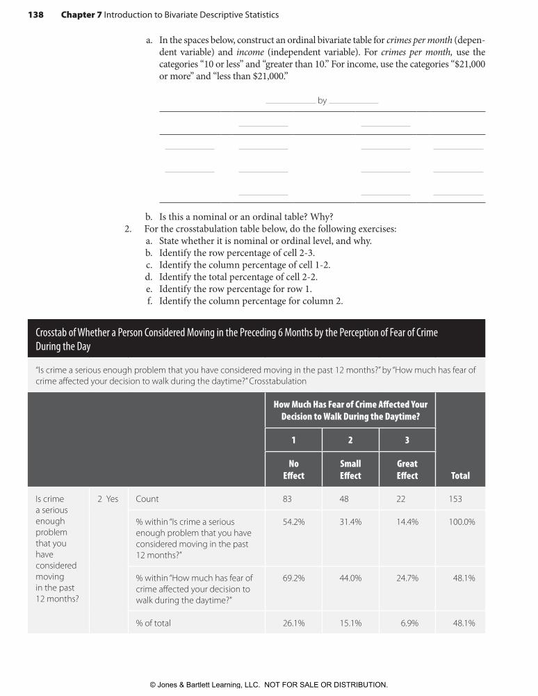
a. State whether it is nominal or ordinal level, and why.b. Identify the row percentage of cell 2-3.c. Identify the column percentage of cell 1-2.d. Identify the total percentage of cell 2-2.e. Identify the row percentage for row 1.f. Identify the column percentage for column 2.
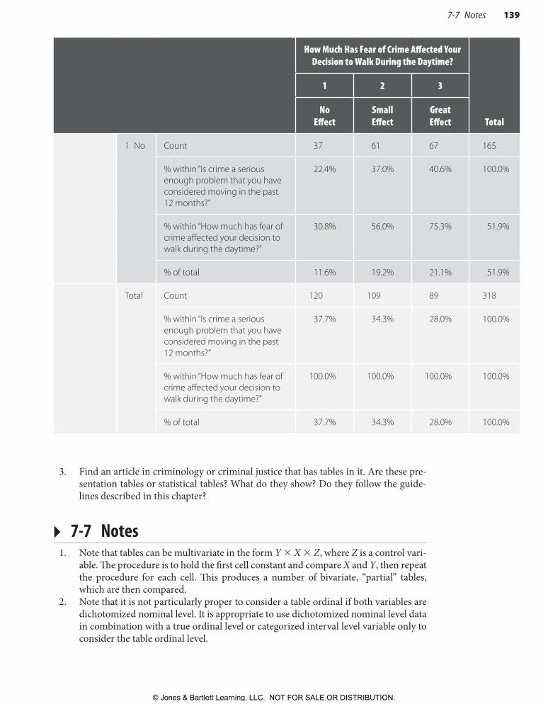
Crosstab of Whether a Person Considered Moving in the Preceding 6 Months by the Perception of Fear of Crime During the Day
“Is crime a serious enough problem that you have considered moving in the past 12 months?” by “How much has fear of crime affected your decision to walk during the daytime?” Crosstabulation
How Much Has Fear of Crime Affected Your Decision to Walk During the Daytime?
Total
1 2 3
NoEffect
SmallEffect
GreatEffect
Is crime a serious enough problem that you have considered moving in the past 12 months?
2 Yes Count 83 48 22 153
% within “Is crime a serious enough problem that you have considered moving in the past 12 months?”
54.2% 31.4% 14.4% 100.0%
% within “How much has fear of crime affected your decision to walk during the daytime?”
69.2% 44.0% 24.7% 48.1%
% of total 26.1% 15.1% 6.9% 48.1%
138 Chapter 7 Introduction to Bivariate Descriptive Statistics
© Jones & Bartlett Learning, LLC. NOT FOR SALE OR DISTRIBUTION.
© Jones & Bartlett Learning, LLCNOT FOR SALE OR DISTRIBUTION
© Jones & Bartlett Learning, LLCNOT FOR SALE OR DISTRIBUTION
© Jones & Bartlett Learning, LLCNOT FOR SALE OR DISTRIBUTION
© Jones & Bartlett Learning, LLCNOT FOR SALE OR DISTRIBUTION
© Jones & Bartlett Learning, LLCNOT FOR SALE OR DISTRIBUTION
© Jones & Bartlett Learning, LLCNOT FOR SALE OR DISTRIBUTION
© Jones & Bartlett Learning, LLCNOT FOR SALE OR DISTRIBUTION
© Jones & Bartlett Learning, LLCNOT FOR SALE OR DISTRIBUTION
© Jones & Bartlett Learning, LLCNOT FOR SALE OR DISTRIBUTION
© Jones & Bartlett Learning, LLCNOT FOR SALE OR DISTRIBUTION
© Jones & Bartlett Learning, LLCNOT FOR SALE OR DISTRIBUTION
© Jones & Bartlett Learning, LLCNOT FOR SALE OR DISTRIBUTION
© Jones & Bartlett Learning, LLCNOT FOR SALE OR DISTRIBUTION
© Jones & Bartlett Learning, LLCNOT FOR SALE OR DISTRIBUTION
© Jones & Bartlett Learning, LLCNOT FOR SALE OR DISTRIBUTION
© Jones & Bartlett Learning, LLCNOT FOR SALE OR DISTRIBUTION
© Jones & Bartlett Learning, LLCNOT FOR SALE OR DISTRIBUTION
© Jones & Bartlett Learning, LLCNOT FOR SALE OR DISTRIBUTION
© Jones & Bartlett Learning, LLCNOT FOR SALE OR DISTRIBUTION
© Jones & Bartlett Learning, LLCNOT FOR SALE OR DISTRIBUTION
3. Find an article in criminology or criminal justice that has tables in it. Are these pre-sentation tables or statistical tables? What do they show? Do they follow the guide-lines described in this chapter?
▸ 7-7 Notes1. Note that tables can be multivariate in the form Y 3 X 3 Z, where Z is a control vari-
able. The procedure is to hold the first cell constant and compare X and Y, then repeat the procedure for each cell. This produces a number of bivariate, “partial” tables, which are then compared.
2. Note that it is not particularly proper to consider a table ordinal if both variables are dichotomized nominal level. It is appropriate to use dichotomized nominal level data in combination with a true ordinal level or categorized interval level variable only to consider the table ordinal level.
How Much Has Fear of Crime Affected Your Decision to Walk During the Daytime?
Total
1 2 3
NoEffect
SmallEffect
GreatEffect
1 No Count 37 61 67 165
% within “Is crime a serious enough problem that you have considered moving in the past 12 months?”
22.4% 37.0% 40.6% 100.0%
% within “How much has fear of crime affected your decision to walk during the daytime?”
30.8% 56.0% 75.3% 51.9%
% of total 11.6% 19.2% 21.1% 51.9%
Total Count 120 109 89 318
% within “Is crime a serious enough problem that you have considered moving in the past 12 months?”
37.7% 34.3% 28.0% 100.0%
% within “How much has fear of crime affected your decision to walk during the daytime?”
100.0% 100.0% 100.0% 100.0%
% of total 37.7% 34.3% 28.0% 100.0%
7-7 Notes 139
© Jones & Bartlett Learning, LLC. NOT FOR SALE OR DISTRIBUTION.