3AI1 MATHEMATICS-III UNIT 1 : LAPLACE TRANSFORM - Laplace ...
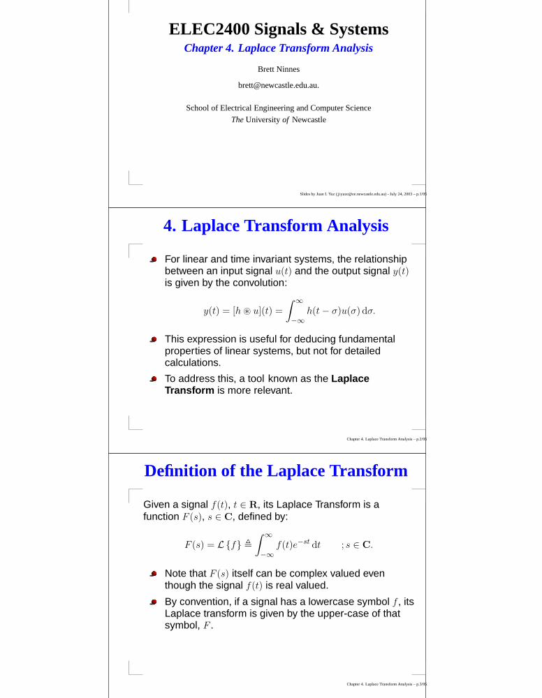
ELEC2400 Signals & SystemsChapter 4. Laplace Transform Analysis
Brett Ninnes
School of Electrical Engineering and Computer Science
The University of Newcastle
Slides by Juan I. Yuz ([email protected]) - July 24, 2003 – p.1/95
4. Laplace Transform Analysis
For linear and time invariant systems, the relationshipbetween an input signal u(t) and the output signal y(t)is given by the convolution:
y(t) = [h ~ u](t) =
∫ ∞
−∞h(t − σ)u(σ) dσ.
This expression is useful for deducing fundamentalproperties of linear systems, but not for detailedcalculations.
To address this, a tool known as the LaplaceTransform is more relevant.
Chapter 4. Laplace Transform Analysis – p.2/95
Definition of the Laplace Transform
Given a signal f(t), t ∈ R, its Laplace Transform is afunction F (s), s ∈ C, defined by:
F (s) = Lf ,
∫ ∞
−∞f(t)e−st dt ; s ∈ C.
Note that F (s) itself can be complex valued eventhough the signal f(t) is real valued.
By convention, if a signal has a lowercase symbol f , itsLaplace transform is given by the upper-case of thatsymbol, F .
Chapter 4. Laplace Transform Analysis – p.3/95

Definition of the Laplace Transform
The previous definition is more correctly called thebilateral Laplace Transform, to distinguish it from themore common used unilateral Laplace Transform:
F (s) = Lf ,
∫ ∞
0−
f(t)e−st dt ; s ∈ C.
In the sequel, we will use only the bilateral LaplaceTransform since it has several advantages:
It does not ignore values of f(t) for t < 0, allowingto consider non-causal systems.It allows a simple and direct link between Fourierand Laplace Transforms to be established.Some fundamental properties of the LaplaceTransform are simpler to state and use.
Chapter 4. Laplace Transform Analysis – p.4/95
Geometric InterpretationLaplace Transform:
F (s) = Lf ,
∫ ∞
−∞f(t)e−st dt ; s ∈ C.
As s = α + jω, then by De Moivre’s Theorem:
e−st = e−(α+jω)t = e−αte−jωt = e−αt (cosωt − j sinωt)
Hence:
F (s)|s=α+jω =
∫ ∞
−∞
f(t)e−αt cos ωt dt − j
∫ ∞
−∞
f(t)e−αt sinωt dt.
Consequently:Real F (s) measures the strength of e−αt cosωt inf(t), andImag F (s) measures the strength of e−αt sin ωt.
Chapter 4. Laplace Transform Analysis – p.5/95
Geometric Interpretation
Depending on α and ω, F (s) = F (α + jω) measures thestrength of various exponentially enveloped andoscillating signals in f(t):
t
e−αt
αα
e−αt
0
t
e−αtReal
t
t
e−αt cos(ωt)e−αt
2π
ω
e−αt
ω
2π
ω
e−αt cos(ωt)
2π
ω
Imaginary
Chapter 4. Laplace Transform Analysis – p.6/95
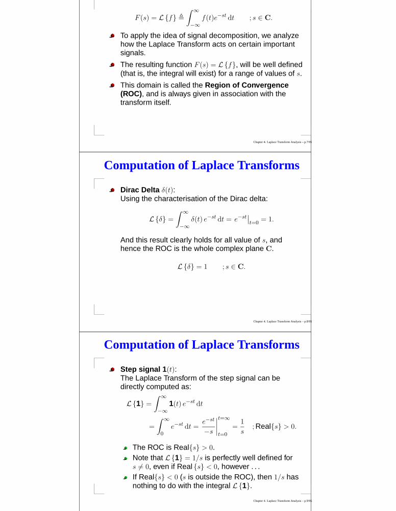
Computation of Laplace Transforms
F (s) = Lf ,
∫ ∞
−∞f(t)e−st dt ; s ∈ C.
To apply the idea of signal decomposition, we analyzehow the Laplace Transform acts on certain importantsignals.
The resulting function F (s) = Lf, will be well defined(that is, the integral will exist) for a range of values of s.
This domain is called the Region of Convergence(ROC), and is always given in association with thetransform itself.
Chapter 4. Laplace Transform Analysis – p.7/95
Computation of Laplace Transforms
Dirac Delta δ(t):Using the characterisation of the Dirac delta:
Lδ =
∫ ∞
−∞δ(t) e−st dt = e−st
∣∣t=0
= 1.
And this result clearly holds for all value of s, andhence the ROC is the whole complex plane C.
Lδ = 1 ; s ∈ C.
Chapter 4. Laplace Transform Analysis – p.8/95
Computation of Laplace Transforms
Step signal 1(t):The Laplace Transform of the step signal can bedirectly computed as:
L1 =
∫ ∞
−∞1(t) e−st dt
=
∫ ∞
0e−st dt =
e−st
−s
∣∣∣∣
t=∞
t=0
=1
s; Reals > 0.
The ROC is Reals > 0.Note that L1 = 1/s is perfectly well defined fors 6= 0, even if Real s < 0, however . . .If Reals < 0 (s is outside the ROC), then 1/s hasnothing to do with the integral L1.
Chapter 4. Laplace Transform Analysis – p.9/95

Computation of Laplace Transforms
Ramp signal r(t):The ramp signal is r(t) = 1(t) · t, then its LaplaceTransform is:
Ls =
∫ ∞
−∞1(t) · t e−st dt
=
∫ ∞
0t e−st dt = . . . =
1
s2; Reals > 0.
Again, the ROC is Reals > 0, since for those valueslimt→∞
e−st = 0 and the above integral is finite.
Chapter 4. Laplace Transform Analysis – p.10/95
Computation of Laplace Transforms
Exponential signal eαt:This signal is defined as f(t) = 1(t) · eαt, α ∈ C, and isprobably the single most important example to study:
F (s) = Lf =
∫ ∞
0eαte−st dt
=
∫ ∞
0e(α−s)t dt =
e(α−s)t
α − s
∣∣∣∣∣
t=∞
t=0
=1
s − α
The ROC is given by Reals > Realα, which isnecessary to ensure:
limt→∞
e(α−s)t → 0
Chapter 4. Laplace Transform Analysis – p.11/95
Computation of Laplace Transforms
Polynomial times Exponential tneαt:For the signal f(t) = 1(t) · teαt:
L
1(t) · teαt
=
∫ ∞
0
teαte−st dt =
∫ ∞
0
[d
dαeαt
]
e−st dt
=d
dα
∫ ∞
0
eαte−st dt =d
dαL
1(t) · eαt
⇒ L
1(t) · teαt
=d
dα
(1
s − α
)
=1
(s − α)2
And for any integer n ≥ 1:
L
1(t) · tneαt
=dn
dαn
(1
s − α
)
=n!
(s − α)n+1
The ROC is Reals > Realα.
Chapter 4. Laplace Transform Analysis – p.12/95

Computation of Laplace Transforms
Cosine cosωt:We consider a pure tone at a frequency of ω [rad/s]:
f(t) = 1(t) · cosωt = 1(t) · 1
2
[ejωt + e−jωt
]
Then:
L1(t) · cosωt =
∫ ∞
0
(cosωt)e−st dt =
∫ ∞
0
1
2
[ejωt + e−jωt
]e−st dt
=1
2
∫ ∞
0
(ejωt
)e−st dt +
1
2
∫ ∞
0
(e−jωt
)e−st dt
=1
2
[1
s − jω+
1
s + jω
]
=s
s2 + ω2
Setting α = jω in the previous result implies that theROC is Reals > 0.
Chapter 4. Laplace Transform Analysis – p.13/95
Computation of Laplace Transforms
Sine sin ωt:Similarly, if we consider a signal:
f(t) = 1(t) · sinωt = 1(t) · 1
2j
[ejωt − e−jωt
]
Then:
L1(t) · sin ωt =
∫ ∞
0
(sinωt)e−st dt =
∫ ∞
0
1
2j
[ejωt − e−jωt
]e−st dt
=1
2j
∫ ∞
0
(ejωt
)e−st dt − 1
2j
∫ ∞
0
(e−jωt
)e−st dt
=1
2j
[1
s − jω− 1
s + jω
]
=ω
s2 + ω2
Again, setting α = jω in the result for 1(t)eαt, impliesthat the ROC is Reals > 0.
Chapter 4. Laplace Transform Analysis – p.14/95
Computation of Laplace Transforms
Exponentially Damped Sinusoidals:Suppose that f(t) is an exponentially dampedsinusoidal signal at ω [rad/s]. Applying the previousdecomposition for cosωt and sin ωt, we have that:
If f(t) = 1(t) · eαt cosωt = 12
[e(α+jω)t + e(α−jω)t
]1(t), then:
L
1(t) · eαt cos ωt
=s − α
(s − α)2 + ω2; Reals > Realα
If f(t) = 1(t) · eαt sinωt = 12j
[e(α+jω)t − e(α−jω)t
]1(t), then:
L
1(t) · eαt sinωt
=ω
(s − α)2 + ω2; Reals > Realα
Chapter 4. Laplace Transform Analysis – p.15/95

Properties of Laplace Transforms
Linearity:For any two signals f(t) and g(t) and any α, β ∈ C, then
Lαf + βg =
∫ ∞
−∞[αf(t) + βg(t)] e−st dt
= α
∫ ∞
−∞f(t)e−st dt + β
∫ ∞
−∞g(t)e−st dt
= αLf + βLg
This is a natural consequence of the linearity of theintegral operator, and the ROC is the intersection ofthe ROC’s of Lf and Lg.
Chapter 4. Laplace Transform Analysis – p.16/95
Properties of Laplace Transforms
Time Shifting:Suppose that a signal f(t) is formed by shifting anothersignal g(t) in time:
f(t) = g(t − T ).
Then, using the change of variable x = t − T in theLaplace Transform definition:
F (s) = Lf =
∫ ∞
−∞g(t − T )e−st dt
= e−sT
∫ ∞
−∞g(x)e−sx dx
= e−sTLg = e−sT G(s).
for all s ∈ ROC of G(s).
Chapter 4. Laplace Transform Analysis – p.17/95
Properties of Laplace Transforms
Time Scaling:If the time-scale of a signal is compressed (expanded),its Laplace Transform is expanded (compressed). Thatis, if:
f(t) = g(αt) ;α ∈ R
then, using the change of variable x = αt:
F (s) ,
∫ ∞
−∞f(t) e−st dt =
∫ ∞
−∞g(αt) e−st dt
=1
α
∫ ∞
−∞g(x) e−xs/α dx
=1
αG
( s
α
)
for all s ∈ ROC of G(s).
Chapter 4. Laplace Transform Analysis – p.18/95
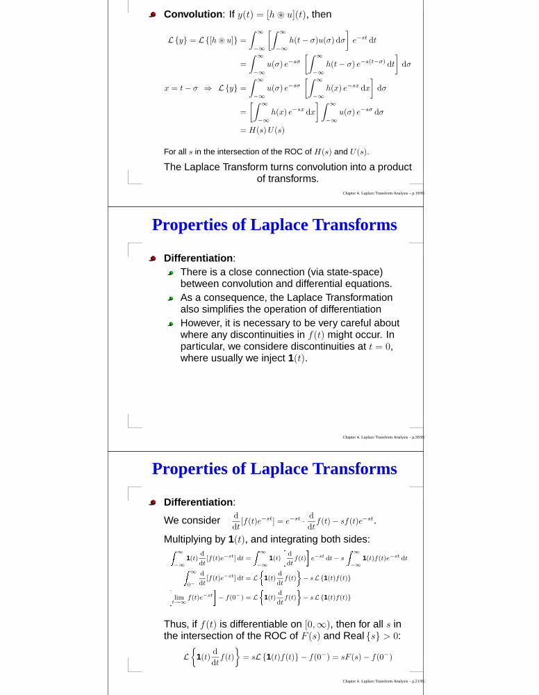
Properties of Laplace Transforms
Convolution: If y(t) = [h ~ u](t), then
Ly = L[h ~ u] =
∫ ∞
−∞
[∫ ∞
−∞
h(t − σ)u(σ) dσ
]
e−st dt
=
∫ ∞
−∞
u(σ) e−sσ
[∫ ∞
−∞
h(t − σ) e−s(t−σ) dt
]
dσ
x = t − σ ⇒ Ly =
∫ ∞
−∞
u(σ) e−sσ
[∫ ∞
−∞
h(x) e−sx dx
]
dσ
=
[∫ ∞
−∞
h(x) e−sx dx
] ∫ ∞
−∞
u(σ) e−sσ dσ
= H(s) U(s)
For all s in the intersection of the ROC of H(s) and U(s).
The Laplace Transform turns convolution into a productof transforms.
Chapter 4. Laplace Transform Analysis – p.19/95
Properties of Laplace Transforms
Differentiation:There is a close connection (via state-space)between convolution and differential equations.As a consequence, the Laplace Transformationalso simplifies the operation of differentiationHowever, it is necessary to be very careful aboutwhere any discontinuities in f(t) might occur. Inparticular, we considere discontinuities at t = 0,where usually we inject 1(t).
Chapter 4. Laplace Transform Analysis – p.20/95
Properties of Laplace Transforms
Differentiation:
We consider d
dt[f(t)e−st] = e−st · d
dtf(t) − sf(t)e−st.
Multiplying by 1(t), and integrating both sides:
∞
−∞
1(t)d
dt[f(t)e−st] dt =
∞
−∞
1(t)
d
dtf(t) e
−st dt − s
∞
−∞
1(t)f(t)e−st dt
∞
0−
d
dt[f(t)e−st] dt = L 1(t)
d
dtf(t) − sL1(t)f(t)
limt→∞
f(t)e−st
− f(0−) = L 1(t)d
dtf(t) − sL1(t)f(t)
Thus, if f(t) is differentiable on [0,∞), then for all s inthe intersection of the ROC of F (s) and Real s > 0:
L
1(t)d
dtf(t)
= sL1(t)f(t) − f(0−) = sF (s) − f(0−)
Chapter 4. Laplace Transform Analysis – p.21/95

Properties of Laplace Transforms
Differentiation:For the 2nd order derivative we have:
L 1(t)d2
dt2f(t) = sL 1(t) ·
d
dtf(t) − lim
t→0−
d
dtf(t)
= s sF (s) − f(0−) −d
dtf(0−) = s2F (s) − sf(0−) −
d
dtf(0−)
And, for higher order derivatives:
L 1(t) ·dn
dtnf(t) = snF (s) − sn−1f(0−) − sn−2 d
dtf(0−) − · · · −
dn−1
dtn−1f(0−)
for all s in the intersection of the ROC of F (s) andReal s > 0.
The Laplace Transform turns differentiation (in the timedomain) into a multiplication by the scalar s.
Chapter 4. Laplace Transform Analysis – p.22/95
Properties of Laplace Transforms
Integration:Using integration by parts (assuming t > t0):
L∫ t
t0
f(σ) dσ
=
∫ ∞
−∞
[∫ t
t0
f(σ) dσ
]
e−st dt
=
∫ ∞
−∞
[∫ t
t0
f(σ) dσ
]d
dt
(e−st
−s
)
dt
=
[e−st
−s
∫ t
t0
f(σ) dσ
]∣∣∣∣
t=∞
t=t0
+1
s
∫ ∞
−∞
f(t) e−st dt
=1
sF (s)
For all s in the intersection of the ROC of Lf andReals > 0.
Chapter 4. Laplace Transform Analysis – p.23/95
Properties of Laplace Transforms
Integration:For the general case, with multiple integrals:
L∫ tn
t0
∫ tn−1
t0
· · ·∫ t2
t0
∫ t1
t0
f(σ) dσ dt1 dt2 · · · dtn−2 dtn−1
=1
snF (s).
For all s in the intersection of the ROC of Lf andReals > 0.
This result is consistent with the Laplace Transformof the step 1(t) and Dirac delta δ(t) signals:
1(t) =
∫ t
−∞
δ(σ) dσ ⇒ L1(t) =1
sLδ =
1
s, Reals > 0
The Laplace Transform turns integration into divisionby the scalar s.
Chapter 4. Laplace Transform Analysis – p.24/95

Properties of Laplace Transforms
Transform of a Product:We have seen that:
L[h ~ u](t) = LhL u = H(s)U(s)
There is a dual result : If h(t) = g(t)f(t), then for anyγ ∈ R such that G(s) and F (s) exist for all s = γ + jωwith ω ∈ (−∞,∞), then:
Lg(t)f(t) = H(s) =1
2πj
∫ γ+j∞
γ−j∞F (s − σ)G(σ) dσ
The Laplace transform turns the product of two signalsinto the convolution of two transforms.
Chapter 4. Laplace Transform Analysis – p.25/95
Properties of Laplace Transforms
Multiplication by eαt:We have seen that:
Lf(t − T ) = e−sTLf = e−sT F (s)
Again, there is a dual result:
Leαtg(t)
=
∫ ∞
−∞
eαtg(t)e−st dt =
∫ ∞
−∞
g(t)e−(s−α)t dt = G(s − α).
For example:
L
1(t) · eαt cos ωt
= L1(t) · cosωt|s:=s−α =s − α
(s − α)2 + ω2
The Laplace Transform turns multiplication by anexponential function in one domain into translation in
the other.
Chapter 4. Laplace Transform Analysis – p.26/95
Properties of Laplace Transforms
Multiplication by t:This is another dual result, straightforward to establish.Given any integer n and for all s in the ROC of Lf:
Ltnf(t) = (−1)ndn
dsnLf = (−1)n
dn
dsnF (s).
For example:
L1(t) · t sinωt = (−1)d
ds
(ω
s2 + ω2
)
=2 ωs
(s2 + ω2)2; Reals > 0.
The Laplace Transform turns differentiation of order nin one domain into multiplication by the domain
variable (s or t) to the power n in the other domain.
Chapter 4. Laplace Transform Analysis – p.27/95

Properties of Laplace Transforms
Initial Value Theorem:We have seen that:
sL1(t) · f(t) − f(0−) = L
1(t) · d
dtf(t)
=
∫ ∞
0−
[d
dtf(t)
]
e−st dt
Taking the limit as Reals → ∞ on both sides:
limReals→∞
sL1(t) · f(t)−f(0−) = limReals→∞
∫ ∞
0−
[d
dtf(t)
]
e−st dt = 0
Therefore, assuming f(t) differentiable on [0,∞), andprovided that ROC of L1(t)f(t) is a half planeReal s > α for some α ∈ R:
limReals→∞
sL1(t) · f(t) = f(0−)
Chapter 4. Laplace Transform Analysis – p.28/95
Properties of Laplace Transforms
Final Value Theorem:Again starting from:
sL1(t) · f(t) − f(0−) =
∞
0−
d
dtf(t) e
−st dt
But taking the limit as s → 0:
lims→0
sF (s) − f(0−) = lims→0
∞
−∞
1(t) ·d
dtf(t)e−st dt =
∞
0−
d
dtf(t)
1
lims→0e−st
dt
= ∞
0−
d
dtf(t) dt = f(∞) − f(0−).
Therefore, provided that L1(t) · f(t) , F (s) isdefined for every s in a region around 0:
lims→0
sF (s) = f(∞)
Chapter 4. Laplace Transform Analysis – p.29/95
Inversion of Laplace Transforms
We need a tool in order to recover a signal f(t) from itsLaplace Transform F (s) = Lf.
The Inverse Laplace Transform is given as:
f(t) = L−1 F ,1
2πj
∫ γ+j∞
γ−j∞F (s)est ds
where γ ∈ R is such that all s ∈ (γ − jω, γ + jω) are inthe Region of Convergence of F (s).
The Inverse Laplace Transform is a linear operation:
L−1 αF + βG = αL−1 F + βL−1 G
for any complex numbers α, β ∈ C
Chapter 4. Laplace Transform Analysis – p.30/95

Contour Integral Formulation
The Inverse Laplace Transform may appear somewhatcomplicated.
In practice, it can be evaluated converting it to acontour integral, which depends just on the residues ofthe integrand.
First, we note that for most Laplace transforms F (s)
lim|s|→∞
|F (s)| = 0 , for example lim|s|→∞
Leat
= lim
|s|→∞
∣∣∣∣
1
s − a
∣∣∣∣= 0
.Then: ∫
ΓF (s)est ds = 0 ; t ≥ 0
where Γ is an infinite radius arc in the complex plane(see next slide).
Chapter 4. Laplace Transform Analysis – p.31/95
Contour Integral Formulation
0
Extension ΓLine Λ = (γ − j∞, γ + j∞)
Imaginary
γ Real
Function F (s)est
Area = f(t) =1
2πj
γ+j∞
γ−j∞
F (s)est ds
Infinite Radius
Defining the contour C = Λ + Γ and for t ≥ 0:
f(t) = L−1 F (s) =1
2πj
∫
Λ
F (s)est ds+1
2πj
∫
Γ
F (s)est ds
︸ ︷︷ ︸
0
=1
2πj
∮
C
F (s)est ds
Chapter 4. Laplace Transform Analysis – p.32/95
Contour Integral Formulation
0
Extension ΓLine Λ = (γ − j∞, γ + j∞)
Imaginary
γ Real
Function F (s)est
Area = f(t) =1
2πj
γ+j∞
γ−j∞
F (s)est ds
Infinite Radius
Provided that |F (s)| → 0 as |s| → ∞, then the InverseLaplace Transform of F (s) may be written as:
f(t) = L−1 F =1
2πj
∮
CF (s)est ds ; t ≥ 0
Chapter 4. Laplace Transform Analysis – p.33/95

Evaluation by Residue Calculation
We will apply Cauchy’s Residue Theorem to computethe inverse Laplace transform:
L−1 F =1
2πj
∮
CF (s)est ds ; t ≥ 0
Firstly,
A pole pk of F (s) is any value such that F (pk) = ±∞.(e.g., F (s) = 1
s−ahas a pole at s = p1 = a)
The residue of F (s) at the pole s = pk is
Ress=pk
F (s) = [(s − pk)F (s)]|s=pk
(
e.g. Ress=a
1s−a
= 1)
Chapter 4. Laplace Transform Analysis – p.34/95
Evaluation by Residue Calculation
(continued)A pole pk of F (s) has multiplicity m if:
F (pk) = ±∞ and
∣∣∣∣lim
s→pk
(s − pk)mF (s)
∣∣∣∣< ∞
Then the residue of F (s) at the pole s = pk is:
Ress=pk
F (s) =1
(m − 1)!
dm−1
dsm−1[(s − pk)mF (s)]
∣∣∣∣s=pk
The Cauchy’s Residue Theorem establishes:
1
2πj
∮
C
G(s) ds =n∑
k=1
Ress=pk
G(s).
where C is a smooth closed curve in C, and G(s) isdifferentiable within C except at isolated poles p1, · · · , pn.
Chapter 4. Laplace Transform Analysis – p.35/95
Evaluation by Residue Calculation
Applying this theorem with G(s) = F (s)est, provides asimple formula for the Inverse Laplace Transform:
Suppose that the poles of F (s) are at points p1, · · · , pn
and that F (s) → 0 as |s| → ∞. Then, for t ≥ 0
f(t) = L−1 F =1
2πj
∮
CF (s)est ds =
n∑
k=1
Ress=pk
[F (s)est
]
where the integration is taken counter-clockwisearound the path C.
Note that the poles of F (s)est are the poles of F (s).
Chapter 4. Laplace Transform Analysis – p.36/95

Evaluation by Residue Calculation
Isolated Poles:If all the poles p1, p2, · · · , pn of F (s) have multiplicitym = 1 each, and lim|s|→∞ |F (s)| = 0, then:
L−1F (s) =n∑
k=1
(s − pk)F (s)∣∣∣s=pk
epkt
Example 1. Suppose that: F (s) =1
s + aThen F (s)est has only one pole at p1 = −a.Provided t ≥ 0 then F (s)est is zero on the infinite arc Γ.Therefore, for t ≥ 0:
f(t) = L−1F (s) = (s + a)F (s)|s=−a e−at = e−at ; t ≥ 0
which agrees with the previously known result.
Chapter 4. Laplace Transform Analysis – p.37/95
Evaluation by Residue Calculation
Isolated Poles.Example 2. Suppose that:
F (s) =1
τs + 1
Then the function F (s)est has only one pole at p1 = −1/τ , and|F (s)| → 0 as |s| → ∞. Therefore, for t ≥ 0:
f(t) = L−1F (s) = (s + 1/τ)1
τs + 1
∣∣∣∣s=−1/τ
e−t/τ
=1
τ
(s + 1/τ)
(s + 1/τ)
∣∣∣∣s=−1/τ
e−t/τ
=1
τe−t/τ ; t ≥ 0
Chapter 4. Laplace Transform Analysis – p.38/95
Evaluation by Residue Calculation
Isolated Poles.Example 3. Suppose that:
F (s) =1
s2 + 3s + 2
Clearly, F (s)est has two poles, p1 = −1 and p2 = −2.Provided t > 0, then (F (s)est) → 0 on the infinite arc Γ.Therefore:
f(t) = L−1F (s) = (s + 1)F (s)|s=−1 e−t + (s + 2)F (s)|s=−2 e−2t
=1
(s + 2)
∣∣∣∣s=−1
e−t +1
(s + 1)F (s)
∣∣∣∣s=−2
e−2t
= e−t − e−2t ; t ≥ 0
Chapter 4. Laplace Transform Analysis – p.39/95
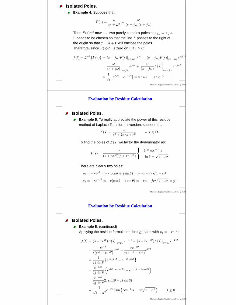
Evaluation by Residue Calculation
Isolated Poles.Example 4. Suppose that:
F (s) =ω
s2 + ω2=
ω
(s − jω)(s + jω)
Then F (s)est now has two purely complex poles at p1,2 = ±jω.Γ needs to be chosen so that the line Λ passes to the right ofthe origin so that C = Λ + Γ will enclose the poles.Therefore, since F (s)est is zero on Γ if t ≥ 0:
f(t) = L−1F (s) = (s − jω)F (s)|s=jω ejωt + (s + jω)F (s)|s=−jω e−jωt
=ω
(s + jω)
∣∣∣∣s=jω
ejωt +ω
(s − jω)F (s)
∣∣∣∣s=−jω
e−jωt
=1
2j
[ejωt − e−jωt
]= sinωt ; t ≥ 0
Chapter 4. Laplace Transform Analysis – p.40/95
Evaluation by Residue Calculation
Isolated Poles.Example 5. To really appreciate the power of this residuemethod of Laplace Transform inversion, suppose that:
F (s) =s
s2 + 2αrs + r2; α, r ∈ R.
To find the poles of F (s) we factor the denominator as:
F (s) =s
(s + rejθ)(s + re−jθ)
θ , cos−1 α
sin θ =√
1 − α2
There are clearly two poles:
p1 = −rejθ = −r(cos θ + j sin θ) = −rα − jr√
1 − α2
p2 = −re−jθ = −r(cos θ − j sin θ) = −rα + jr√
1 − α2 = p1
Chapter 4. Laplace Transform Analysis – p.41/95
Evaluation by Residue Calculation
Isolated Poles.Example 5. (continued)Applying the residue formulation for t ≥ 0 and with p1 = −rejθ :
f(t) = (s + rejθ)F (s)∣∣s=p1
e−p1t + (s + re−jθ)F (s)∣∣s=p1
e−p1t
=rejθ
r(ejθ − e−jθ)ep1t +
re−jθ
r(e−jθ − ejθ)ep1t
=1
2j sin θ
ejθep1t − e−jθep1t
=e−rαt
2j sin θ
ej(θ−rt sin θ) − e−j(θ−rt sin θ)
=e−rαt
2j sin θ2j sin(θ − rt sin θ)
=1√
1 − α2e−rαt sin
(
cos−1 α − rt√
1 − α2)
; t ≥ 0
Chapter 4. Laplace Transform Analysis – p.42/95
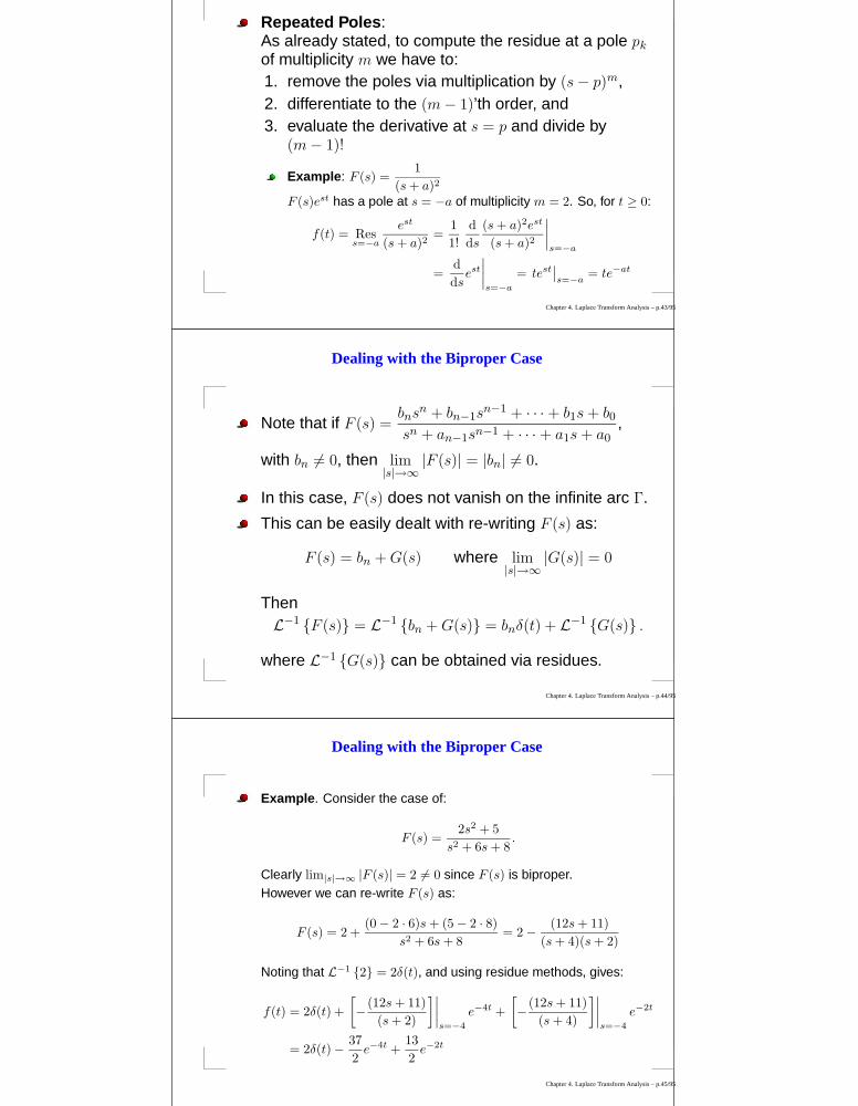
Evaluation by Residue Calculation
Repeated Poles:As already stated, to compute the residue at a pole pk
of multiplicity m we have to:1. remove the poles via multiplication by (s − p)m,2. differentiate to the (m − 1)’th order, and3. evaluate the derivative at s = p and divide by
(m − 1)!
Example: F (s) =1
(s + a)2
F (s)est has a pole at s = −a of multiplicity m = 2. So, for t ≥ 0:
f(t) = Ress=−a
est
(s + a)2=
1
1!
d
ds
(s + a)2est
(s + a)2
∣∣∣∣s=−a
=d
dsest
∣∣∣∣s=−a
= test∣∣s=−a
= te−at
Chapter 4. Laplace Transform Analysis – p.43/95
Dealing with the Biproper Case
Note that if F (s) =bnsn + bn−1s
n−1 + · · · + b1s + b0
sn + an−1sn−1 + · · · + a1s + a0,
with bn 6= 0, then lim|s|→∞
|F (s)| = |bn| 6= 0.
In this case, F (s) does not vanish on the infinite arc Γ.
This can be easily dealt with re-writing F (s) as:
F (s) = bn + G(s) where lim|s|→∞
|G(s)| = 0
ThenL−1 F (s) = L−1 bn + G(s) = bnδ(t) + L−1 G(s) .
where L−1 G(s) can be obtained via residues.
Chapter 4. Laplace Transform Analysis – p.44/95
Dealing with the Biproper Case
Example. Consider the case of:
F (s) =2s2 + 5
s2 + 6s + 8.
Clearly lim|s|→∞ |F (s)| = 2 6= 0 since F (s) is biproper.However we can re-write F (s) as:
F (s) = 2 +(0 − 2 · 6)s + (5 − 2 · 8)
s2 + 6s + 8= 2 − (12s + 11)
(s + 4)(s + 2)
Noting that L−1 2 = 2δ(t), and using residue methods, gives:
f(t) = 2δ(t) +
[
− (12s + 11)
(s + 2)
]∣∣∣∣s=−4
e−4t +
[
− (12s + 11)
(s + 4)
]∣∣∣∣s=−4
e−2t
= 2δ(t) − 37
2e−4t +
13
2e−2t
Chapter 4. Laplace Transform Analysis – p.45/95

Causality of the Inverse Laplace Transform
Recall that:
f(t) = L−1 F ,1
2πj
∫ γ+j∞
γ−j∞
F (s)est ds
where γ ∈ R is such that s ∈ (γ − jω, γ + jω) is inside theROC of F (s).
ROC of Laplace Transforms considered so far are ofthe form:
ROC F (s) = s ∈ C : Real s > Real α
where α is such that the poles of F (s) lie to the left ofReal α.
Chapter 4. Laplace Transform Analysis – p.46/95
Causality of the Inverse Laplace Transform
Then, for t ≥ 0:∫
Λ
F (s)est ds =
∫
Λ
F (s)est ds
+
∫
Γ
F (s)est ds
=
∮
C
F (s)est ds
Using Cauchy’s Theorem:
f(t) = L−1 F (s) =n∑
k=1
[
Ress=pk
F (s)est
]
0
Ims
γ
Res
Contour C
Poles of F (s)
Line Λ
Arc Γ
Chapter 4. Laplace Transform Analysis – p.47/95
Causality of the Inverse Laplace Transform
If t < 0:
The infinite arc Γmust be changed(else, est → ∞)
Therefore,F (s) contains nopoles within C.
Hence,
f(t) =1
2πj
∮
C
F (s)est ds = 0
Contour C
0 Resγ
Ims
Arc ΓLine Λ
Poles of F(s)
Chapter 4. Laplace Transform Analysis – p.48/95

Causality of the Inverse Laplace Transform
Therefore, the general causality principle for LaplaceTransforms is:
(Causal signals) Provided |F (s)| → 0 as |s| → ∞,and that the ROC of F (s) has the forms ∈ C : Real s > α,α ∈ R. Then:
L−1 F (s) = f(t) = 0 for t < 0.
(Anti-causal signals) Provided |G(s)| → 0 as|s| → ∞, and that the ROC of G(s) has the forms ∈ C : Real s < α,α ∈ R. Then:
L−1 G(s) = g(t) = 0 for t > 0
Chapter 4. Laplace Transform Analysis – p.49/95
Causality of the Inverse Laplace Transform
For example,Consider the anti-causal signal (α > 0):
g(t) =
eαt ; t ≤ 0
0 ; t > 0⇒ G(s) =
∫ 0
−∞
eαte−st d =−1
s − α
and ROC G(s) = s ∈ C : Real s < Real α.However, the causal signal:
f(t) =
0 ; t ≤ 0
−eαt ; t > 0⇒ F (s) = −
∫ ∞
0
eαte−st d =−1
s − α
and ROC F (s) = s ∈ C : Real s > Real α.
Chapter 4. Laplace Transform Analysis – p.50/95
Dealing with Time Translations
According to the time-shifting property:
Lf(t + T ) = esTLf(t) = esT F (s).
This transforms do not satisfy |esT F (s)| → 0 as|s| → ∞, thus we have to
Initially remove any esT term,Obtain the Inverse Laplace tranform, and thenApply the necessary time translation.
Example:
Consider F (s) =e−2s
s − α. We have that L−1
1
s − α
= 1(t) · eαt,
and the e−2s term corresponds to a time delay, hence:
L−1
e−2s
s − α
= 1(t − 2) · eα(t−2).
Chapter 4. Laplace Transform Analysis – p.51/95
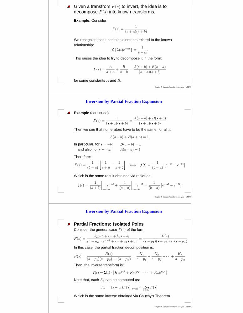
Inversion by Partial Fraction Expansion
Given a transfrom F (s) to invert, the idea is todecompose F (s) into known transforms.
Example. Consider:
F (s) =1
(s + a)(s + b)
We recognise that it contains elements related to the knownrelationship:
L
1(t)e−αt
=1
s + α.
This raises the idea to try to decompose it in the form:
F (s) =A
s + a+
B
s + b=
A(s + b) + B(s + a)
(s + a)(s + b)
for some constants A and B.
Chapter 4. Laplace Transform Analysis – p.52/95
Inversion by Partial Fraction Expansion
Example (continued)
F (s) =1
(s + a)(s + b)=
A(s + b) + B(s + a)
(s + a)(s + b)
Then we see that numerators have to be the same, for all s:
A(s + b) + B(s + a) = 1.
In particular, for s = −b: B(a − b) = 1
and also, for s = −a: A(b − a) = 1
Therefore:
F (s) =1
(b − a)
[1
s + a− 1
s + b
]
⇐⇒ f(t) =1
(b − a)
[e−at − e−bt
]
Which is the same result obtained via residues:
f(t) =1
(s + b)
∣∣∣∣s=−a
e−at +1
(s + a)
∣∣∣∣s=−b
e−bt =1
(b − a)
[e−at − e−bt
]
Chapter 4. Laplace Transform Analysis – p.53/95
Inversion by Partial Fraction Expansion
Partial Fractions: Isolated PolesConsider the general case F (s) of the form:
F (s) =bmsm + · · · + b1s + b0
sn + an−1sn−1 + · · · + a1s + a0=
B(s)
(s − p1)(s − p2) · · · (s − pn)
In this case, the partial fraction decomposition is:
F (s) =B(s)
(s − p1)(s − p2) · · · (s − pn)=
K1
s − p1+
K2
s − p2+ · · ·+ Kn
s − pn
Then, the inverse transform is:
f(t) = 1(t) ·[K1e
p1t + K2ep2t + · · · + Knepnt
]
Note that, each Ki can be computed as:
Ki = (s − pi)F (s)|s=pi = Ress=pi
F (s).
Which is the same inverse obtained via Cauchy’s Theorem.
Chapter 4. Laplace Transform Analysis – p.54/95
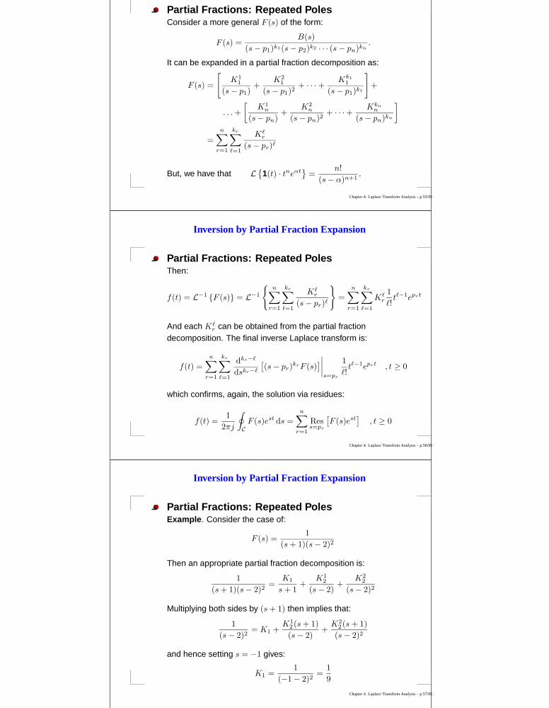
Inversion by Partial Fraction Expansion
Partial Fractions: Repeated PolesConsider a more general F (s) of the form:
F (s) =B(s)
(s − p1)k1(s − p2)k2 · · · (s − pn)kn.
It can be expanded in a partial fraction decomposition as:
F (s) =
[
K11
(s − p1)+
K21
(s − p1)2+ · · · + Kk1
1
(s − p1)k1
]
+
. . . +
[K1
n
(s − pn)+
K2n
(s − pn)2+ · · · + Kkn
n
(s − pn)kn
]
=n∑
r=1
kr∑
`=1
K`r
(s − pr)`
But, we have that L
1(t) · tneαt
=n!
(s − α)n+1.
Chapter 4. Laplace Transform Analysis – p.55/95
Inversion by Partial Fraction Expansion
Partial Fractions: Repeated PolesThen:
f(t) = L−1 F (s) = L−1
n∑
r=1
kr∑
`=1
K`r
(s − pr)`
=n∑
r=1
kr∑
`=1
K`r
1
`!t`−1eprt
And each K`r can be obtained from the partial fraction
decomposition. The final inverse Laplace transform is:
f(t) =n∑
r=1
kr∑
`=1
dkr−`
dskr−`
[(s − pr)
krF (s)]∣∣∣∣s=pr
1
`!t`−1eprt , t ≥ 0
which confirms, again, the solution via residues:
f(t) =1
2πj
∮
C
F (s)est ds =n∑
r=1
Ress=pr
[F (s)est
], t ≥ 0
Chapter 4. Laplace Transform Analysis – p.56/95
Inversion by Partial Fraction Expansion
Partial Fractions: Repeated PolesExample. Consider the case of:
F (s) =1
(s + 1)(s − 2)2
Then an appropriate partial fraction decomposition is:
1
(s + 1)(s − 2)2=
K1
s + 1+
K12
(s − 2)+
K22
(s − 2)2
Multiplying both sides by (s + 1) then implies that:
1
(s − 2)2= K1 +
K12 (s + 1)
(s − 2)+
K22 (s + 1)
(s − 2)2
and hence setting s = −1 gives:
K1 =1
(−1 − 2)2=
1
9
Chapter 4. Laplace Transform Analysis – p.57/95

Inversion by Partial Fraction Expansion
Partial Fractions: Repeated PolesExample (continued)Starting from:
F (s) =1
(s + 1)(s − 2)2=
K1
s + 1+
K12
(s − 2)+
K22
(s − 2)2
and multiplying both sides by (s − 2)2 also implies that:
1
(s + 1)=
K1(s − 2)2
s + 1+ K1
2 (s − 2) + K22
which when evaluated at s = 2 gives:
K22 =
1
(2 + 1)=
1
3
Chapter 4. Laplace Transform Analysis – p.58/95
Inversion by Partial Fraction Expansion
Partial Fractions: Repeated PolesExample (continued)Finally, also from:
F (s) =1
(s + 1)(s − 2)2=
K1
s + 1+
K12
(s − 2)+
K22
(s − 2)2
differentiating both sides with respect to s, implies that:
−1
(s + 1)2=
2K1(s − 2)(s + 1) − K1(s − 2)2
(s + 1)2+ K1
2
which evaluated at s = 2 implies:
K12 =
−1
(2 + 1)2= −1
9.
Therefore:
F (s) =1
9· 1
s + 1− 1
9· 1
(s − 2)+
1
6· 2
(s − 2)2
⇐⇒ f(t) = 1(t) ·[1
9e−t − 1
9· e2t +
1
6· te2t
]
Chapter 4. Laplace Transform Analysis – p.59/95
Inversion by Partial Fraction Expansion
Given the equivalence, the residue-based methodappears to be superior to partial fractiondecomposition:
It does not require memorization of any LaplaceTransform results;It can be used even when there are some elementsnot recognisable from available transform tables;It directly exposes why a pole at p in a transformF (s) implies a term ept;The calculations involved computing residues areidentical to those in computing partial fractionexpansion coefficients.
Chapter 4. Laplace Transform Analysis – p.60/95
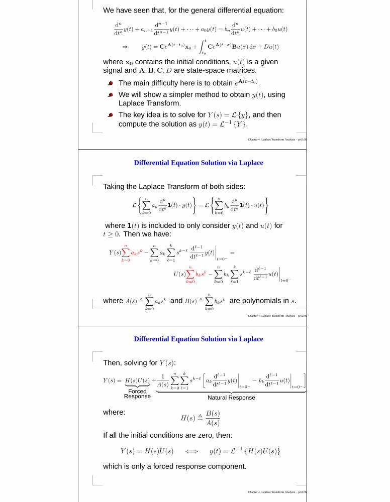
Differential Equation Solution via Laplace
We have seen that, for the general differential equation:
dn
dtny(t) + an−1
dn−1
dtn−1y(t) + · · · + a0y(t) = bn
dn
dtnu(t) + · · · + b0u(t)
⇒ y(t) = CeA(t−t0)x0 +
∫ t
t0
CeA(t−σ)Bu(σ) dσ + Du(t)
where x0 contains the initial conditions, u(t) is a givensignal and A,B,C, D are state-space matrices.
The main difficulty here is to obtain eA(t−t0).
We will show a simpler method to obtain y(t), usingLaplace Transform.
The key idea is to solve for Y (s) = Ly, and thencompute the solution as y(t) = L−1 Y .
Chapter 4. Laplace Transform Analysis – p.61/95
Differential Equation Solution via Laplace
Taking the Laplace Transform of both sides:
L
n∑
k=0
akdk
dtk1(t) · y(t)
= L
n∑
k=0
bkdk
dtk1(t) · u(t)
where 1(t) is included to only consider y(t) and u(t) fort ≥ 0. Then we have:
Y (s)
n∑
k=0
aksk −n∑
k=0
ak
k∑
`=1
sk−` d`−1
dt`−1y(t)
∣∣∣∣t=0−
=
U(s)
n∑
k=0
bksk −n∑
k=0
bk
k∑
`=1
sk−` d`−1
dt`−1u(t)
∣∣∣∣t=0−
where A(s) ,
n∑
k=0
aksk and B(s) ,
n∑
k=0
bksk are polynomials in s.
Chapter 4. Laplace Transform Analysis – p.62/95
Differential Equation Solution via Laplace
Then, solving for Y (s):
Y (s) = H(s)U(s)︸ ︷︷ ︸
ForcedResponse
+1
A(s)
n∑
k=0
k∑
`=1
sk−`
[
akd`−1
dt`−1y(t)
∣∣∣∣t=0−
− bkd`−1
dt`−1u(t)
∣∣∣∣t=0−
]
︸ ︷︷ ︸
Natural Response
where:H(s) ,
B(s)
A(s)
If all the initial conditions are zero, then:
Y (s) = H(s)U(s) ⇐⇒ y(t) = L−1 H(s)U(s)
which is only a forced response component.
Chapter 4. Laplace Transform Analysis – p.63/95

Differential Equation Solution via Laplace
Example: First Order Case
d
dty(t) + a0y(t) = b0u(t) ; y(0−) = y0.
Taking Laplace transform of both sides:
sY (s) − y(0−) + a0Y (s) = b0U(s).
so that: Y (s) =
(b0
s + a0
)
U(s)
︸ ︷︷ ︸
Forced Response
+1
(s + a0)y(0−)
︸ ︷︷ ︸
Natural ResponseIf u(t) = 1(t) ⇐⇒ U(s) = 1/s, then:
Y (s) =b0
(s + a0)· 1
s+
1
(s + a0)y(0−)
⇒ y(t) =
[b0
a0
[1 − e−a0t
]+ y(0−)e−a0t
]
1(t)
Chapter 4. Laplace Transform Analysis – p.64/95
Differential Equation Solution via Laplace
Example: Second Order CaseTo compute the evolution of vC(t) after the switch is closed, adifferential equation model for vC(t) is required.
+
+t = 0
vR(t) vL(t)
R = 50Ω L = 10H
vC(t)
C = 25000µFV?
By Kirchoff’s Voltage Law
vR(t) + vL(t) + vC(t) = V?
By Kirchoff’s Current Law:
iR(t) = iL(t) = iC(t)
And for the resistor, the inductorand the capacitor, we have that:
vR(t) = R iR(t)
vL(t) = Ld
dtiL(t)
iC(t) = Cd
dtvC(t)
Chapter 4. Laplace Transform Analysis – p.65/95
Differential Equation Solution via Laplace
Example: Second Order Case (continued)Therefore, making some substitutions:
vR(t) = R iR(t) = R iC(t) = RCd
dtvC(t)
vL(t) = Ld
dtiR(t) = L
d
dtiC(t) = LC
d2
dt2vC(t)
Inserting this into the KVL equation:
RCd
dtvC(t) + LC
d2
dt2vC(t) + vC(t) = V?
⇐⇒ d2
dt2vC(t) +
R
L
d
dtvC(t) +
1
LCvC(t) =
1
LCV?
Taking Laplace Transforms of both sides, LvC(t) = VC(s), gives:
s2VC (s) − svC(0−) −
d
dtvC(0−) +
R
L sVC(s) − vC (0−) +1
LCVC (s) =
1
LC
V?
s
Chapter 4. Laplace Transform Analysis – p.66/95
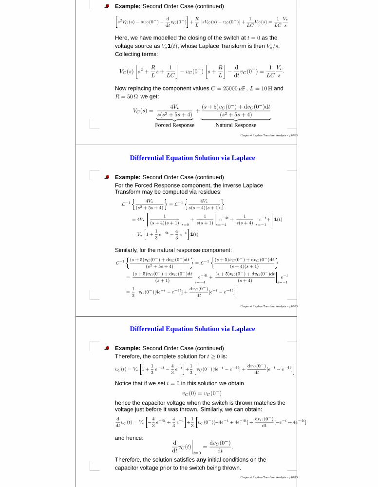
Differential Equation Solution via Laplace
Example: Second Order Case (continued)
s2VC (s) − svC(0−) −
d
dtvC(0−) +
R
L sVC(s) − vC (0−) +1
LCVC (s) =
1
LC
V?
s
Here, we have modelled the closing of the switch at t = 0 as thevoltage source as V?1(t), whose Laplace Transform is then V?/s.Collecting terms:
VC(s)
[
s2 +R
Ls +
1
LC
]
− vC(0−)
[
s +R
L
]
− d
dtvC(0−) =
1
LC
V?
s.
Now replacing the component values C = 25000 µF , L = 10 H andR = 50 Ω we get:
VC(s) =4V?
s(s2 + 5s + 4)︸ ︷︷ ︸
Forced Response
+(s + 5)vC(0−) + dvC(0−)dt
(s2 + 5s + 4)︸ ︷︷ ︸
Natural Response
Chapter 4. Laplace Transform Analysis – p.67/95
Differential Equation Solution via Laplace
Example: Second Order Case (continued)For the Forced Response component, the inverse LaplaceTransform may be computed via residues:
L−1
4V?
(s2 + 5s + 4) = L−1
4V?
s(s + 4)(s + 1)
= 4V?
1
(s + 4)(s + 1)
s=0
+1
s(s + 1)
s=−4
e−4t +1
s(s + 4)
s=−1
e−t+ 1(t)
= V? 1 +1
3e−4t −
4
3e−t
1(t)
Similarly, for the natural response component:
L−1
(s + 5)vC(0−) + dvC (0−)dt
(s2 + 5s + 4) = L−1
(s + 5)vC(0−) + dvC (0−)dt
(s + 4)(s + 1)
=(s + 5)vC (0−) + dvC(0−)dt
(s + 1)
s=−4
e−4t +(s + 5)vC(0−) + dvC (0−)dt
(s + 4)
s=−1
e−t
=1
3 vC (0−)[4e−t − e−4t] +dvC (0−)
dt[e−t − e−4t]
Chapter 4. Laplace Transform Analysis – p.68/95
Differential Equation Solution via Laplace
Example: Second Order Case (continued)Therefore, the complete solution for t ≥ 0 is:
vC(t) = V? 1 +1
3e−4t −
4
3e−t
+1
3 vC(0−)[4e−t − e−4t] +dvC (0−)
dt[e−t − e−4t]
Notice that if we set t = 0 in this solution we obtain
vC(0) = vC(0−)
hence the capacitor voltage when the switch is thrown matches thevoltage just before it was thrown. Similarly, we can obtain:
d
dtvC(t) = V? −
4
3e−4t +
4
3e−t
+1
3 vC (0−)[−4e−t + 4e−4t] +dvC (0−)
dt[−e−t + 4e−4t]
and hence:d
dtvC(t)
∣∣∣∣t=0
=dvC(0−)
dt.
Therefore, the solution satisfies any initial conditions on thecapacitor voltage prior to the switch being thrown.
Chapter 4. Laplace Transform Analysis – p.69/95

Differential Equation Solution via Laplace: Initial Conditions
We have seen that for 1(t) ,
0 ; t < 0
1 ; t ≥ 0
L
1(t) · d
dtf(t)
= sL1(t) · f(t) +
∫ ∞
0−
d
dt[f(t)e−st] dt
= sL1(t) · f(t) − f(0−)
where t = 0−, a point infinitessimally smaller than (tothe left of) the time t = 0.
If we define a new function 1+(t) ,
0 ; t ≤ 0
1 ; t > 0
then: L
1+(t) · d
dtf(t)
= sL1(t) · f(t) − f(0+)
Therefore, Laplace Transform can also handle initialcondition at t = 0+, if given.
Chapter 4. Laplace Transform Analysis – p.70/95
Differential Equation Solution via Laplace: Initial Conditions
Note that f(0+) − f(0−) =
∫ 0+
0−
d
dt[f(t)e−st] dt.
Then, if ddt
f(t) is bounded in t ∈ (0−, 0+) (e.g. f(t) 6= 1(t)),then the integral is zero, and f(0+) = f(0−) = f(0).
In general: If dk
dtkf(t) ; ∀k = 0, . . . , n exist on (0,∞)
then for all s in ROC F (s) and Real s > 0:
L
1+(t) · dn
dtnf(t)
= sn L1+(t) · f(t) −n∑
k=1
sn−k dk−1
dtk−1f(0+)
Furthermore, if the derivatives are also bounded, then:
L
1+(t) · dn
dtnf(t)
= L
1(t) · dn
dtnf(t)
= sn L1(t) · f(t) −n∑
k=1
sn−k dk−1
dtk−1f(0−)
Chapter 4. Laplace Transform Analysis – p.71/95
Differential Equation Solution via Laplace: Initial Conditions
Example: Schock absorber revisited.Assuming that the car mass, shock absorber spring stiffness anddamper viscosity are:
m = 1000 kg, ks = 2000 N/m, kd = 3000 Ns/m
Then, the relationship between car height y(t) and road height u(t)
is given as:d2
dt2y(t) + 3
d
dty(t) + 2y(t) = 3
d
dtu(t) + 2u(t)
Suppose further initial conditions: y(0−) = −0.5 ,d
dty(0−) = −1
and a unit step input u(t) = 1(t), so that: u(0−) = 0 ,d
dtu(0−) = 0
Taking Laplace Transforms of both sides:
s2Y (2) − sy(0−) −d
dty(0−) + 3sY (s) − 3y(0−) + 2Y (s) = 3sU(s) − 3u(0−) + 2U(s)
⇒ (s2 + 3s + 2)Y (s) − (s + 3)y(0−) −d
dt(0−) = (3s + 2)U(s) − 3u(0−)
Chapter 4. Laplace Transform Analysis – p.72/95
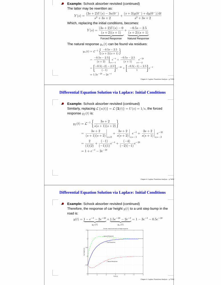
Differential Equation Solution via Laplace: Initial Conditions
Example: Schock absorber revisited (continued)The latter may be rewritten as:
Y (s) =(3s + 2)U(s) − 3u(0−)
s2 + 3s + 2+
(s + 3)y(0−) + dy(0−)/dt
s2 + 3s + 2
Which, replacing the initial conditions, becomes:
Y (s) =(3s + 2)U(s) − 0
(s + 2)(s + 1)︸ ︷︷ ︸
Forced Response
+−0.5s − 2.5
(s + 2)(s + 1)︸ ︷︷ ︸
Natural Response
The natural response yn(t) can be found via residues:
yn(t) = L−1
−0.5s − 2.5
(s + 2)(s + 1)
=−0.5s − 2.5
(s + 2)
s=−1
e−t +−0.5s − 2.5
(s + 1)
s=−2
e−2t
=
−0.5(−2) − 2.5
(−1) e−2t +
−0.5(−1) − 2.5
1 e−t
= 1.5e−2t − 2e−t
Chapter 4. Laplace Transform Analysis – p.73/95
Differential Equation Solution via Laplace: Initial Conditions
Example: Schock absorber revisited (continued)Similarly, replacing Lu(t) = L1(t) = U(s) = 1/s, the forcedresponse yf (t) is:
yf (t) = L−1
3s + 2
s(s + 1)(s + 2)
=3s + 2
(s + 1)(s + 2)
∣∣∣∣s=0
+3s + 2
s(s + 2)
∣∣∣∣s=−1
e−t +3s + 2
s(s + 1)
∣∣∣∣s=−2
e−2t
=2
(1)(2)+
(−1)
(−1)(1)e−t +
(−4)
(−2)(−1)e−2t
= 1 + e−t − 2e−2t
Chapter 4. Laplace Transform Analysis – p.74/95
Differential Equation Solution via Laplace: Initial Conditions
Example: Schock absorber revisited (continued)Therefore, the response of car height y(t) to a unit step bump in theroad is:
y(t) = 1 − e−t − 2e−2t
︸ ︷︷ ︸
yf (t)
+ 1.5e−2t − 2e−t
︸ ︷︷ ︸
yn(t)
= 1 − 3e−t − 0.5e−2t
0 1 2 3 4 5 6−1
−0.5
0
0.5
1
1.5
Time (s)
Car
hei
ght (
m)
Forced, natural and total car height response
←Natural Response
←Forced Response
←Total Response
Chapter 4. Laplace Transform Analysis – p.75/95
Differential Equation Solution via Laplace: Initial Conditions
Example: Schock absorber revisited (continued)Therefore, the response of car height y(t) to a unit step bump in theroad is:
y(t) = 1 − e−t − 2e−2t
︸ ︷︷ ︸
yf (t)
+ 1.5e−2t − 2e−t
︸ ︷︷ ︸
yn(t)
= 1 − 3e−t − 0.5e−2t
Notice that the initial condition specification:
y(0−) = −0.5,d
dty(0−) = −1
is also met by the natural response yn(t) = 1.5e−2t − 2e−t att = 0+, but not by the total response y(t) = yf (t) + yn(t).
This is because the model used involves the input derivativewhich, for the unit step u(t) = 1(t), is discontinuous at t = 0.
It is possible to interpret the derivative of 1(t) as a Dirac deltaδ(t), which allows instantaneous changes in y(t) and dy(t)/dt
at t = 0−.Chapter 4. Laplace Transform Analysis – p.76/95
Differential Equation Solution via Laplace: Initial Conditions
Example: Schock absorber revisited (continued)To underline the latter point, consider the case of the normal (atrest) car height being y(t) = 1m, and up until time t = 0 it isdepressed to y(t) = 0m, being released at t = 0. The appropriateinitial conditions are:
y(0+) = 0,d
dty(0+) = 0.
The differential equation model is the same and the input will still beu(t) = 1(t).The only difference is that the initial conditions are now specified att = 0+ rather than at t = 0−.Therefore, we obtain:
Y (s) =(3s + 2)U(s) − 3u(0+)
s2 + 3s + 2+
(s + 3)y(0+) + dy(0+)/dt
s2 + 3s + 2
Chapter 4. Laplace Transform Analysis – p.77/95
Differential Equation Solution via Laplace: Initial Conditions
Example: Schock absorber revisited (continued)Replacing the initial conditions, and u(0+) = 1 (u(t) = 1(t)):
Y (s) =(3s + 2)1/s − 3
s2 + 3s + 2=
2
s(s + 1)(s + 2)
Therefore:
y(t) = L−1
2
s(s + 1)(s + 2)
=2
(s + 1)(s + 2)
∣∣∣∣s=0
+2
s(s + 2)
∣∣∣∣s=−1
e−t +2
s(s + 1)
∣∣∣∣s=−2
e−2t
=2
(1)(2)+
2
(−1)(1)e−t +
2
(−2)(−1)e−2t
= 1 − 2e−t + e−2t
Chapter 4. Laplace Transform Analysis – p.78/95
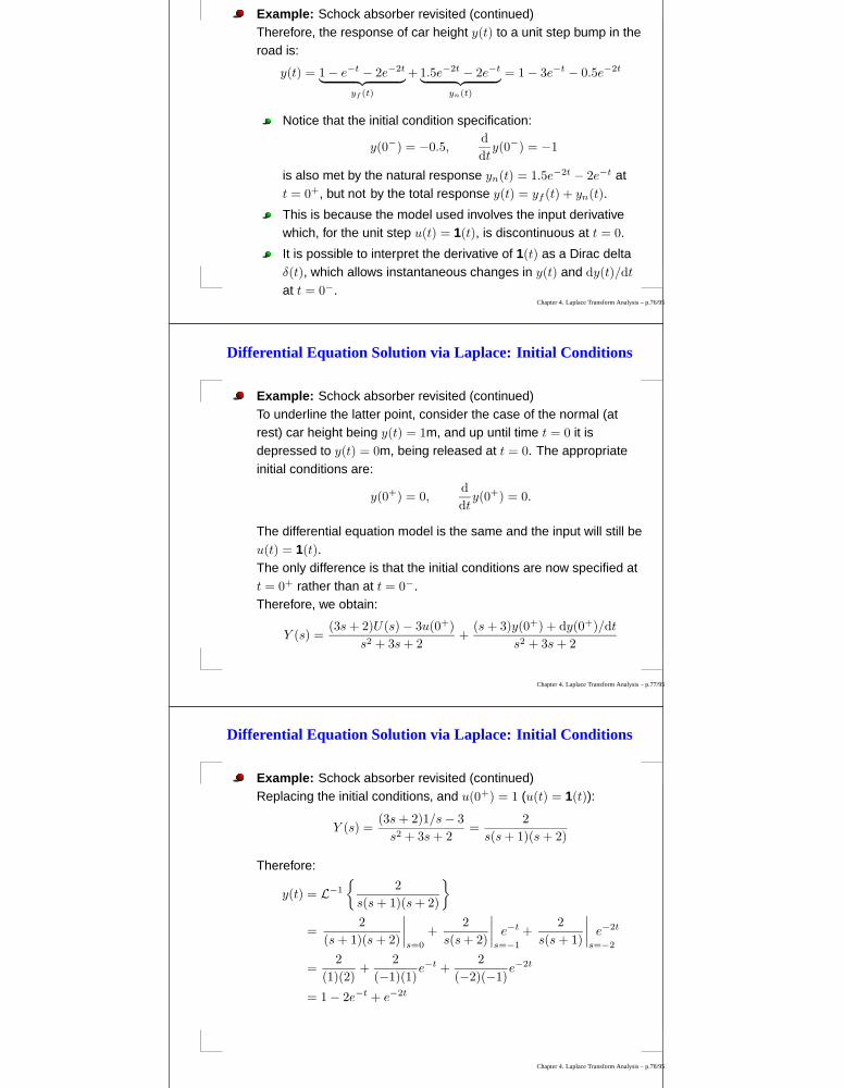
Differential Equation Solution via Laplace: Initial Conditions
Example: Schock absorber revisited (continued)Now, notice that the solution
y(t) = 1 − 2e−t + e−2t
at t = 0+, does satisfy the initial condition also specified at t = 0+.
0 1 2 3 4 5 60
0.1
0.2
0.3
0.4
0.5
0.6
0.7
0.8
0.9
1
Time (s)
Car
hei
ght (
m)
Car height response
Chapter 4. Laplace Transform Analysis – p.79/95
The System Transfer Function
Considering zero initial conditions, we have seen that:
Ly = Y (s) = H(s)U(s)
where H(s) =B(s)
A(s)=
b0 + b1s + . . . + bnsn
a0 + a1s + . . . + sn
is called the transfer function of the system. If thepolynomials A(s) and B(s) are factorized, then:
H(s) =K(s − z1)(s − z2) · · · (s − zm)
(s − p1)(s − p2) · · · (s − pn).
zkk=1,...,m are called the zeros of H(s) (∈ C).
pkk=1,...,n are called the poles of H(s) (∈ C).K is a constant
Chapter 4. Laplace Transform Analysis – p.80/95
The System Transfer Function and State Space Models
We recall that a system can be expressed instate-space form:
d
dtx(t) = Ax(t) + Bu(t)
y(t) = Cx(t) + Du(t).
Taking Laplace Transforms, assuming x(0) = 0:
sX(s) = AX(s) + BU(s)
Y (s) = CX(s) + DU(s).
ThenY (s) = C [sI− A]−1
BU(s) + DU(s)
=(C [sI − A]−1
B + D)
︸ ︷︷ ︸
H(s)
U(s)
Chapter 4. Laplace Transform Analysis – p.81/95
The System Transfer Function and State Space Models
Example: Consider the 2nd order differential equation
d2
dt2y(t) + a1
d
dty(t) + a0y(t) = b1
d
dtu(t) + b0u(t).
Clearly H(s) =b1s + b0
s2 + a1s + a0, and the state-space matrices are:
A =
−a1 1
−a0 0
, B =
b1
b0
, C =[
1 0]
, D = 0
Then, (sI−A)−1
=
s + a1 −1
a0 s
−1
=1
s(s + a1) + a0
s 1
−a0 s + a1
Therefore, using H(s) = C [sI−A]−1
B + D:
H(s) =
(1
s2 + a1s + a0
)[
1 0]
s 1
−a0 s + a1
b1
b0
=b1s + b0
s2 + a1s + a0
Chapter 4. Laplace Transform Analysis – p.82/95
The System Transfer Function
The latter example raises a connection between theeigenvalues of A and the poles of H(s).
The point is that [sI − A]−1 contains terms, all of whichhave det(sI −A) as a dividing factor.
Therefore, since
H(s) = C [sI− A]−1B + D
then the poles of H(s) satisfy
det(sI −A) = det(λI−A) = 0
But, these values of s are equal to the eigenvaluesλk of the matrix A.
Chapter 4. Laplace Transform Analysis – p.83/95
The System Transfer Function
Then, for a system with state space representation:
d
dtx(t) = Ax(t) + Bu(t)
y(t) = Cx(t) + Du(t)
and hence transfer function representation
H(s) = C [sI− A]−1B + D
=K(s − z1)(s − z2) · · · (s − zm)
(s − p1)(s − p2) · · · (s − pn)
the poles p1, · · · , pn of H(s) are the eigenvaluesλ1, · · · , λn of A.
Chapter 4. Laplace Transform Analysis – p.84/95
Stability and the Transfer FunctionRecall that a system described by:
dn
dtny(t) + . . . + a0y(t) = bm
dm
dtmu(t) + . . . + b0u(t).
or (equivalently) by the state space model:d
dtx(t) = Ax(t) + Bu(t)
y(t) = Cx(t) + Du(t).
is asymptotically stable ⇐⇒ the eigenvaluesλ1, . . . , λn of A satisfy Real λk < 0.
Then, using the transfer function representation:
H(s) =b0 + b1s + . . . + bnsn
a0 + a1s + . . . + ansn=
K(s − z1)(s − z2) . . . (s − zm)
(s − p1)(s − p2) . . . (s − pn).
the system is asymptotically stable ⇐⇒ the polesp1, . . . , pn of H(s) satisfy Real pk < 0.
Chapter 4. Laplace Transform Analysis – p.85/95
Transfer Function and Impulse Response
Recall that the relationship between y(t) and u(t), can bedescribed through the convolution with the impulseresponse h(t):
y(t) = [h ~ u](t) =
∫ ∞
−∞h(σ)u(t − σ) dσ
⇒ Y (s) = Ly = Lh ~ u = H(s)U(s)
The transfer function H(s) of a system is the LaplaceTransform of its impulse response h(t).
Example:Consider the system
d2
dt2y(t) + 3
d
dty(t) + 2y(t) = 3
d
dtu(t) + 2u(t)
The associated transfer function is H(s) = 3s+2s2+3s+2 = 3s+2
(s+1)(s+2)
Therefore, the impulse response is h(t) = L−1 H = 4e−t − e−t
Chapter 4. Laplace Transform Analysis – p.86/95
Laplace Transforms in Electrical Circuits
We have seen that Laplace Transform methods areuseful to compute the response of linear systemsdescribed by a differential equation.
However, it is possible to directly derive transferfunction descriptions in s, without an intermediatedifferential equation modelling step.
For example, for the fundamental electrical circuitcomponents:
(Resistor) vR(t) = RiR(t) ⇒ VR(s) = RIR(s)
(Inductor) vL(t) = Ld
dtiL(t) ⇒ VL(s) = sLIL(s) − LiL(0−)
(Capacitor) iC(t) = Cd
dtvC(t) ⇒ VC(s) =
1
sCIC(s) +
1
svC(0−)
Chapter 4. Laplace Transform Analysis – p.87/95

Laplace Transforms in Electrical Circuits
When any initial energy storage in the elements isconsidered to be zero (i.e., iL(0−) = vC(0−) = 0), thenwe have the general relationship:
V (s) = ZI(s)
where:(Resistor) VR(s) = RIR(s) ⇒ Z = RI
(Inductor) VL(s) = sLIL(s) ⇒ Z = sL
(Capacitor) VC(s) =1
sCIC(s) ⇒ Z =
1
sC
That is, in the Laplace Transform s-domain, allelements are represented as a generalised resistance,called impedance and denoted by Z.
Chapter 4. Laplace Transform Analysis – p.88/95
Laplace Transforms in Electrical Circuits
+
+
+
+
+ +
+
+
i(t)
i(t)
i(t)
C
R
L
Z =1
sC
Z = R
Z = sLLiL(0)
I(s)
I(s)
I(s)
v(t)
v(t)
v(t)
1
svC(0)
V (s) = RI(s)
V (s) =1
sCI(s) +
1
svc(0
−)
V (s) = sL I(s) − Lil(0−)
Chapter 4. Laplace Transform Analysis – p.89/95
Laplace Transforms in Electrical Circuits
Kirchoff’s Laws:These laws are inherited in the s-domain, due to thelinearity of the Laplace transform:
(KCL) At any circuit node:∑
k
ik(t) = 0 ⇐⇒ L
∑
k
ik(t)
=∑
k
Lik(t)
=∑
k
Ik(s) = 0
And similarly, (KVL) around any circuit mesh:∑
k
vk(t) = 0 ⇐⇒∑
k
Vk(s) = 0
Chapter 4. Laplace Transform Analysis – p.90/95

Laplace Transforms in Electrical Circuits
Series Combination:
+
+
+ +
Z1
Z2
I(s)
V (s) V (s)
I(s)
Zeq = Z1 + Z2
V1(s)
V2(s)
By Kirchoff’s voltage law
V (s) = V1(s) + V2(s) = Z1I(s) + Z2I(s) = ZeqI(s)
where, as indicated Zeq , Z1 + Z2.
Chapter 4. Laplace Transform Analysis – p.91/95
Laplace Transforms in Electrical Circuits
Parallel Combination:
+ +
Z2Z1
I(s)
V (s) V (s)
I1(s) I2(s)
Zeq =Z1Z2
Z1 + Z2
I(s)
By Kirchoff’s current law:
I(s) = I1(s) + I2(s) =V (s)
Z1+
V (s)
Z2= V (s)
[1
Z1+
1
Z2
]
and therefore1
Zeq=
1
Z1+
1
Z2⇐⇒ Zeq =
Z1Z2
Z1 + Z2= Z1‖Z2
Chapter 4. Laplace Transform Analysis – p.92/95
Laplace Transforms in Electrical Circuits
Voltage Division:
+
+
I(s)
Z1
Z2
V (s)
V2(s)
By the result on seriesimpedances:
I(s) =V (s)
Z1 + Z2.
However, V2(s) = Z2I(s)so that
V2(s) =
[Z2
Z1 + Z2
]
V (s).
This is known as voltagedivision.
Chapter 4. Laplace Transform Analysis – p.93/95

Laplace Transforms in Electrical Circuits
Example: 1st Order Op-Amp Circuit
+
−+ +
− −
+ −
+
−+ +
− −
−+
Ri
Vc(s)
Rf
Vo(s)
1
sC
V+(s)
V−(s)
vo(t)
vc(t)
Ri
i1(t)
Rfi3(t)
i2(t)
v−
v+vi(t) Vi(s)
Using the principle of voltage division:
V−(s) =(Vo(s) − Vi(s))Ri
Ri + Rf‖ 1sC
+ Vi(s)
By the negative feedback (assuming ideal Op-Amp): V−(s) = V+(s) = 0
ThenRi
Ri + Rf‖ 1sC
Vo(s) =
(Ri
Ri + Rf‖ 1sC
− 1
)
Vi(s)
Chapter 4. Laplace Transform Analysis – p.94/95
Laplace Transforms in Electrical Circuits
Example: 1st Order Op-Amp Circuit
+
−+ +
− −
+ −
+
−+ +
− −
−+
Ri
Vc(s)
Rf
Vo(s)
1
sC
V+(s)
V−(s)
vo(t)
vc(t)
Ri
i1(t)
Rfi3(t)
i2(t)
v−
v+vi(t) Vi(s)
Therefore:
Vo(s) =
(
1 − Ri + Rf‖ 1sC
Ri
)
Vi(s) = −(
Rf‖1
sC
)1
RiVi(s)
= −(
Rf · 1/sCRf + 1/sC
)1
RiVi(s) = −
(Rf
Ri(sCRf + 1)
)
︸ ︷︷ ︸
H(s)
Vi(s)
Chapter 4. Laplace Transform Analysis – p.95/95