Applications of the Homogenization Method to Flow andTransport in Porous MediaUlrich HornungFak. f. Informatik, UniBwMD-85577 Neubiberg, Germanyulrich@informatik.unibw-muenchen.deXiao Shutie (Ed.) \Summer School on Flow and Transport in Porous Media.Beijing, China, 8-26 August 1988" World Scienti�c, Singapore (1992) 167-222Copyright c 1992 by World Scienti�c Publishing

0

1Contents1 Introduction 22 Elliptic Equations 52.1 A First Example : : : : : : : : : : : : : : : : : : : : : : : : : : : : : 52.2 An Elliptic Boundary Value Problem : : : : : : : : : : : : : : : : : : 62.3 Formal Asymptotic Expansion : : : : : : : : : : : : : : : : : : : : : 72.4 Layered Media : : : : : : : : : : : : : : : : : : : : : : : : : : : : : : 102.5 Energy Estimate Proof : : : : : : : : : : : : : : : : : : : : : : : : : : 112.6 Non-Scalar Coe�cients : : : : : : : : : : : : : : : : : : : : : : : : : : 152.7 Non-Uniformly Oscillating Coe�cients : : : : : : : : : : : : : : : : : 162.8 Non-Uniformly Periodic Media : : : : : : : : : : : : : : : : : : : : : 172.9 Nonlinear Problems : : : : : : : : : : : : : : : : : : : : : : : : : : : 193 Media with Obstacles 213.1 Solid Obstacles : : : : : : : : : : : : : : : : : : : : : : : : : : : : : : 213.2 Thin Obstacles : : : : : : : : : : : : : : : : : : : : : : : : : : : : : : 243.3 Non-Uniformly Periodic Obstacles : : : : : : : : : : : : : : : : : : : 244 Parabolic Equations 254.1 Fractured Media : : : : : : : : : : : : : : : : : : : : : : : : : : : : : 254.2 Convergence Proof : : : : : : : : : : : : : : : : : : : : : : : : : : : : 304.3 Miscible Displacement In uenced by Mobile and Immobile Water : : 354.4 Flow and Transport in Unsaturated Fractured Media : : : : : : : : : 365 Problems on the Pore Scale 385.1 Derivation of Darcy's Law : : : : : : : : : : : : : : : : : : : : : : : : 385.2 Immiscible Displacement Problems : : : : : : : : : : : : : : : : : : : 415.3 Elastic Porous Media : : : : : : : : : : : : : : : : : : : : : : : : : : : 445.4 Chromatography : : : : : : : : : : : : : : : : : : : : : : : : : : : : : 445.5 Semipermeable Membranes : : : : : : : : : : : : : : : : : : : : : : : 445.6 Heterogeneous Catalysis : : : : : : : : : : : : : : : : : : : : : : : : : 466 Further Aspects 48

2 Homogenization1 IntroductionPorous media are a typical example for media with microstructure. On the scale ofpores there are not only the solid matrix and the space of the pores, but also thedi�erent phases of liquids and gases �lling the pores and all the interfaces betweenthese phases. This situation has been described very often by soil physicists, soilchemists and chemical engineers. Pictures illustrating possible con�gurations canbe found in every textbook in these �elds.Science is far from understanding all phenomena taking place on the pore scale.Let us only mention that there is more than only uid ow, namely also interfacialforces play an important role. Furthermore, in the vicinity of the surfaces of thesolid matrix (its geometry can be extremely complicated) adsorption processes, thespecial e�ects of very thin �lms, electric forces, and catalytic recations make ageneral theory di�cult.Nevertheless, for quite some time big e�ort has been invested into answering thequestion of how to formulate laws on a scale that is larger than the pore scale and tojustify these laws from "�rst principles". I.e., to perform what is know as the averag-ing process, see, e.g., [46], [48] [49] [50], [66] and [92]. A recent survey articel is [76].Using the words of this paper one wants to start from certain di�erential equationsthat are assumed to be valid on the micro-scale and - using special techniques - totransform them into equations on the macro-scale.In the seventies mathematicians have developed a new method called homoge-nization. This method has two major aspects: (a) a theoretical and (b) a practialaspect. (a) From a theoretical point of view one studies partial di�erential equa-tions with coe�cients that are higly oscillatory, not necessarly arbitrarily, but eitherperiodically or in a well de�ned sense randomly (or stochastically). Homogenizationperforms certain limits of the solutions of these equations and determines equationswhich the limits are solution of. Textbooks on this subject are [17] [14] and [78].A more abstract theory is contained in [36] and [8]. Important contributions to thetheory can be found in [11], [12], [13] [73], [74]. (b) From a practical point of viewwhat one does is to consider on a large scale media with microstructure, to averageout the physical and chemical processes on the small scale and to calculate e�ectiveproperties of the media. The volume [44] contains a collection of papers devoted toapplications. Especially in elasticity theory there is a large number of papers on thissubject, see [86], [31], and [59].After early attempts to set up a theory (see [65]) a �rst important step in apply-ing the method of homogenization to porous media was done in 1980 in the paper[90] (see also [61]). There a mathematically rigorous proof was presented of derivingDarcy's law from the assumption that the Stokes equations hold on the pore scale.The theorem given there is applicable to steady ow of a single uid in a periodicmedium the solid matrix of which is diconnected. A formal derivation of the sameresult has been published in the same year in [57], see also [62]. In the meantime this

Introduction 3result has been generalized in several ways. The paper [70] deals with nonhomoge-neous boundary conditions. In [1] the geometry has been generalized to connectedmedia, i.e., to cases where the porous matrix itself is connected in space, and notonly the pore space. In [2] it was shown that certain assumptions made on the porescale can lead to di�erent types of equations on the large scale, such as Brinkman'slaw etc. The Navier-Stokes equations were taken into consideration in the paper[68]. Flow around bubbles was considered in [63]Since the method has proved to be very powerful, a variety of applications tomore complicated situations have been published. Miscible displacement problemswere studied in [24] [25] [67] [69] [71]. A related problem is that of hydrodynamicdispersion. The papers [18] [19] [27] [28] [47] [83] investigate this e�ect in periodicmedia. Thermal ow was studied in [42] and [43].The present work is both an introduction and a survey on the subject, see also[39]. In section 2.1 we motivate the procedure by giving a very simple exampleof a layered medium. Since everybody is familiar with this situation, it is easy todemonstrate what is behind this problem. The rest of the section 2 is devoted to thehomogenization of elliptic problems with periodic coe�cients. The formal procedureof asymptotic expansions and also the convergence proof using energy estimates aregiven.In the section 3 media are introduced that have a spatially periodic array ofobstacles. In the space left by the obstacles one studies di�erential equations. The�rst examples are elliptic equations.The section 4 shows that for time dependent problems the method of homog-enization may lead to non-local equations. The crucial point is how to scale themicro-equations. In certain cases the macro-equations may be of integro-di�erentialtype. This situation is by no means arti�cial. That kind of problems has beenstudied in the �eld of oil reservoir simulation for quite some time, see [15] and [5]and [37]. The models are called double porosity models. They apply to problemsof aggregated soils and also to fractured rocks. But also the soil physicists havestudied this type of models, see [16]. Interesting applications are those to mobileand immobile water. The problems are of great theoretical interest, see [88].The section 5 presents a formal derivation of Darcy's law. Further, following theapproach of [10] an attempt is made to derive the model for immiscible displacementin porous media. The drawback here is that certian assumptions of periodicity haveto be made that are not really realistic. Finally, two relatively new problems arepresented. Firstly, the problem of heterogeneous catalysis. In this case, adsoprtionof chemical species is considered and also chemicals reactions that take place on thesurfaces of the porous matrix. Secondly, reactive transport through an array of cellswith semipermeable membranes is described.The last section 6 of this work gives a short outlook onto further problems and

4 Homogenizationsome open questions.

Elliptic Equations 52 Elliptic Equations2.1 A First ExampleIn the unit square f(x1; x2) : 0 < x1; x2 < 1g in R2 we study a di�usion processgoverned by r � (a"(x)ru"(x)) = 0:We make the assumption that a" is a function of x2 only and is periodic withperiodicity length ", in other words we assume thata"(x1; x2) = a(x2" )with a �xed 1-periodic function a : R ! R. This means that we have a layeredmedium in which we want to calculate the e�ective properties. Naturally, we expectthat in an averaged sense the medium can be described by a di�usion equation ofthe type r � (Dru0) = 0 (1)where D is a tensor of the form D = �a 00 a� ! :The easiest way to �nd the numbers �a and a� is to study two simple boundary valueproblems, namely the following.Case 1: 8><>: u = 0; x1 = 0u = 1; x1 = 1@�u = 0; x2 = 0 or = 1Here one has u"(x1; x2) = u0(x1; x2) with u0(x1; x2) = x1 for all " and hence a"ru" =a"~e1 with ~e1 = (1; 0). Therefore, the total ux through the square in x1-direction isZ 10 a"~e1 � ru" dx2 = Z 10 a"(x2) dx2 = Z 10 a(�) d�:This quantity equals to �a, since we have equation 1 independently of ".Case 2: 8><>: u = 0; x2 = 0u = 1; x2 = 1@�u = 0; x1 = 0 or = 1Here one obtains by a simple calculationu"(x1; x2) = u0(x1; x2) + "�2(x2" )

6 Homogenizationwhere u0(x1; x2) = x2 and�2(y2) = a� Z y20 d�a(�) � y2 with a� = 1R 10 d�a(�) :One gets immediately a"ru" = a�~e2:Therefore, the totals ux through the square isZ 10 a"~e2 � ru" dx1 = Z 10 a�dx1 = a�:In this case we see again equation 1. In the next section we are going to see how togive a unifying theory for these two cases.2.2 An Elliptic Boundary Value ProblemWe start from the following problem. Let be a bounded domain in Rn withsmooth boundary @. Then we study the family of boundary value problems( r � (a"(x)ru"(x)) + f(x) = 0; x 2 ;u(x) = uD(x); x 2 @: (2)We assume that the coe�cient a" is rapidly oscillating, i.e. that it is of the forma"(x) = a(x" ) (3)for all x 2 , where the function a is Z-periodic in Rn with periodicity cell Z =fy = (y1; : : : ; yn) : 0 < yi < 1 for i = 1; : : : ; ng and " is a scale parameter. Forsmaller and smaller " the coe�cient a" oscillates more and more rapidly, and thequestion is natural what the solution u" does in the limit " ! 0. We just mentionthat the weak form of problem 2 is(a"ru";r') � (f; ') = 0for all test functions ' on with 'j@ = 0. Here have used the L2-scalar producton (u; v) = Z u(x)v(x) dx:

Elliptic Equations 72.3 Formal Asymptotic ExpansionIn order to derive the limit problem in a formal way one starts from the ansatz thatthe unknown function u" has a power series expansion with respect to " of the formu"(x) = u0(x; y) + "u1(x; y) + "2u2(x; y) + : : : ; (4)where the coe�cient functions ui(x; y) are Z-periodic with respect to the variabley = x" (it is only in this context that superscripts denote powers of "). The derivativesobey the law r = rx + 1"ry;where the subscripts indicate the partial derivatives with respect to x and y resp.Therefore, from equation 2 one gets immediately the formula"�2ry � (a(y)ryu0(x; y))+"�1(ry � (a(y)ryu1(x; y)) +ry � (a(y)rxu0(x; y))+a(y)rx � ryu0(x; y)))+"0(ry � (a(y)ryu2(x; y) + a(y)rxu1(x; y))+a(y)rx � ryu1(x; y) + a(y)rx � rxu0(x; y))+"1(: : :) + : : :+ f(x) = 0: (5)The next step consists in comparing the coe�cients of the di�erent "-powers in thisequation. The term with "�2 givesry � (a(y)ryu0(x; y)) = 0 for y 2 Z:Since u0(x; y) is Z-periodic in the variable y, we obtain that u0(x; y) = u0(x) is afunction of x alone independently of y. Using this, the term with "�1 in equation 5gives ry � (a(y)ryu1(x; y)) = �ry � (a(y)rxu0(x)) for y 2 Z:At this point one expresses the function u1(x; y) in terms of the function u0(x). Theway to do this is to �rst use the obvious identityrxu0(x) = nXj=1 ~ej@xju0(x):Therefore, we can writery � (a(y)ryu1(x; y)) = � nXj=1@yja(y)@xju0(x) for y 2 Z:

8 HomogenizationNow for j = 1; : : : ; n let �j(y) be a Z-periodic solution of the cell-problemry � (a(y)ry�j(y)) = �ry � (a(y)~ej) for y 2 Z (6)the weak form of which is (a(r�j + ~ej);r')Z = 0for all Z-periodic test functions ' on Z.Using these functions �j(y) we can give a solution formula for u1(x; y), namelyu1(x; y) = nXj=1�j(y)@xju0(x) + u1(x);where u1(x) is independent of y. Di�erentiating this gives immediatelyryu1(x; y) = nXj=1ry�j(y)@xju0(x): (7)We proceed further and look at the term with "0 in equation 5. We getry � (a(y)ryu2(x; y) + a(y)rxu1(x; y))+a(y)rx � ryu1(x; y) + a(y)rx � rxu0(x) + f(x) = 0 for y 2 Z:We integrate this identity over Z and obtainZZ ry � (a(y)ryu2(x; y) + a(y)rxu1(x; y)) dy+ ZZ a(y)rx � ryu1(x; y)dy+ ZZ a(y)dy �xu0(x) + f(x) = 0; (8)since the volume of Z is unity. We integrate the �rst integral by parts and getZZ ry � (a(y)ryu2(x; y) + a(y)rxu1(x; y)) dy= Z@Z ~� � (a(y)ryu2(x; y) + a(y)rxu1(x; y)) dy:This boundary integral vanishes because of the Z-periodicity of the functions u2(x; y)and u1(x; y). For the second term in equation 8 we use equation 7 and getrx � ryu1(x; y) = nXi;j=1 @yi�j(y)@xixju0(x):

Elliptic Equations 9In this way we obtain from equation 8nXi;j=1 ZZ a(y)@yi�j(y)@xixju0(x) + ZZ a(y)dy �xu0(x) + f(x) = 0:It is convenient to introduce the abbreviationdij = RZ a(y)(�ij + @yi�j(y)) dy;with which we get the �nal resultnXi;j=1 dij@xixju0(x) + f(x) = 0:This elliptic di�erential equation is the homogenized limit of the equation in problem2. For short we simplify the notation and writenXi;j=1dij@iju(x) + f(x) = 0:Using the tensor D = (dij)i;j we sum up and get the following statement.Proposition 1 The di�erential operator r� (Dru(x)) is the homogenization of theoperator family r � (a"(x)ru"(x)), i.e., the homogenization of problem 2 is( r � (Dru(x)) + f(x) = 0; x 2 ;u(x) = uD(x); x 2 @: (9)Remark: This techniques using a power series with two scales goes back to J. Keller(see, e.g. [57]). We just write down the weak form of this problem. On gets(Dru;r') � (f; ') = 0for all test functions ' on with 'j@ = 0.It has to be emphasized that the coe�cients in the equation we have got byhomogenization are in general not diagonal, or, in other words, we have derived anequation that describes an anisotropic medium. However, in general, the tensor Dis symmetric and positive de�nite.Proposition 2 (a) The tensor D is symmetric.(b) If the coe�cient a in equation 3 satis�esa(y) � � > 0 for all y 2 Z;then D is positive de�nite.

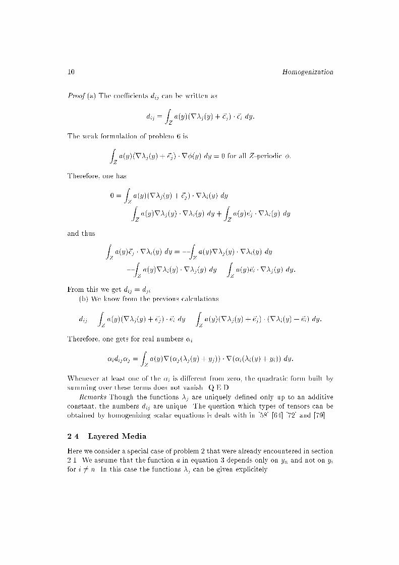
10 HomogenizationProof (a) The coe�cients dij can be written asdij = ZZ a(y)(r�j(y) + ~ej) � ~ei dy:The weak formulation of problem 6 isZZ a(y)(r�j(y) + ~ej) � r�(y) dy = 0 for all Z-periodic �:Therefore, one has0 = ZZ a(y)(r�j(y) + ~ej) � r�i(y) dy= ZZ a(y)r�j(y) � r�i(y) dy + ZZ a(y)~ej � r�i(y) dyand thus ZZ a(y)~ej � r�i(y) dy = � ZZ a(y)r�j(y) � r�i(y) dy= � ZZ a(y)r�i(y) � r�j(y) dy = ZZ a(y)~ei � r�j(y) dy:From this we get dij = dji.(b) We know from the previous calculationsdij = ZZ a(y)(r�j(y) + ~ej) � ~ei dy = ZZ a(y)(r�j(y) + ~ej) � (r�i(y) + ~ei) dy:Therefore, one gets for real numbers �i�idij�j = ZZ a(y)r(�j(�j(y) + yj)) � r(�i(�i(y) + yi)) dy:Whenever at least one of the �i is di�erent from zero, the quadratic form built bysumming over these terms does not vanish. Q.E.D.Remarks Though the functions �j are uniquely de�ned only up to an additiveconstant, the numbers dij are unique. The question which types of tensors can beobtained by homogenizing scalar equations is dealt with in [58] [64] [72] and [79].2.4 Layered MediaHere we consider a special case of problem 2 that were already encountered in section2.1. We assume that the function a in equation 3 depends only on yn and not on yifor i 6= n. In this case the functions �j can be given explicitely.

Elliptic Equations 11Proposition 3 (a) If a(y1; : : : ; yn) = ~a(yn), then solutions of equation 6 are givenby �n(y1; : : : ; yn) = R yn0 d�~a(�)R 10 d�~a(�) � ynand �j = 0 for j 6= n.(b) In this case the coe�cients dij are given bydij = ( a�; i = j = n;�a�ij ; elsewith a� = R 10 d�~a(�) and �a = R 10 ~a(�)d�.Proof The formulas are easily veri�ed by di�erentation and integration. Q.E.D.Remark The physical meaning of part (b) of the proposition is that the e�ectiveconductivity or di�usivity of a layered medium is given by the arithmetic mean in thedirections parallel to the layers but by the geometric mean in the direction normalto the layers. This fact is analogous to the rules that apply to electric resistanceswhich are connected in series or parallel; see, e.g. Lurie and Cherkaev [64]; see also[23].2.5 Energy Estimate ProofThe purpose of this chapter is to show that equation 9 holds in the interior of in astrict sense. The essential part of the proof is to show estimates in certain functionspaces that are satis�ed by the solutions u" independently of ". For this purpose wemake the following assumption:0 < �0 � a(y) � �1 <1 for all y 2 Z:First we introduce some convenient notations. The usual scalar product of H =L2() and its norm are denoted by(:; :) and k:k:Whenever the domain of integration is di�erent from , this will be indicated by anappropriate subscript, e.g., (�; )Z = ZZ �(y) (y)dy:We use the function spacesV = W 1;2() = H1() and V0 = W 1;20 () = H10();and the space of test functions D = C10 (). The weak form of problem 2 is(a"ru";r�) = (f; �) for all � 2 V0: (10)

12 HomogenizationLemma 1 The norms ku"kV are uniformly bounded independently of ".Proof We assume that the boundary data have been extended to a function uD 2 V .Then we get from equation 10(a"ru";r(u" � uD)) = (f; u" � uD)and therefore �0kru"k2 � (a"ru";ru")� j(a"ru";ruD)j+ j(f; u" � uD)j� j(a"ru";ruD)j+ kfk(ku"k+ kuDk)� �1j(ru";ruD)j+ C1kru"k+ C2� C3kru"k+ C2and thus kru"k � C:Q.E.D.We need a basic fact about weak convergence.Lemma 2 Let g 2 L2(Z) be periodically extended to all Rn and g"(x) = g(x" ). Theng" * g weakly in H; where g = ZZ g(y) dy:Proof: Without loss of generality we can assume g = 0: Let � 2 C1(�); then wecan write Z g"(x)�(x)dx = Xk2K Z"Zk g"(x)�(x) dxwith a index set K the number jKj of elements of which satis�es jKj"n � C: Let astep function � be de�ned by�(x) = Z"Zk �(~x) d~x; if x 2 "Zk ;then we can writeZ g"(x)�(x) dx = Xk2K Z"Zk g"(x)(�(x)� �(x)) dx+ Xk2K Z"Zk g"(x) dx �(x):

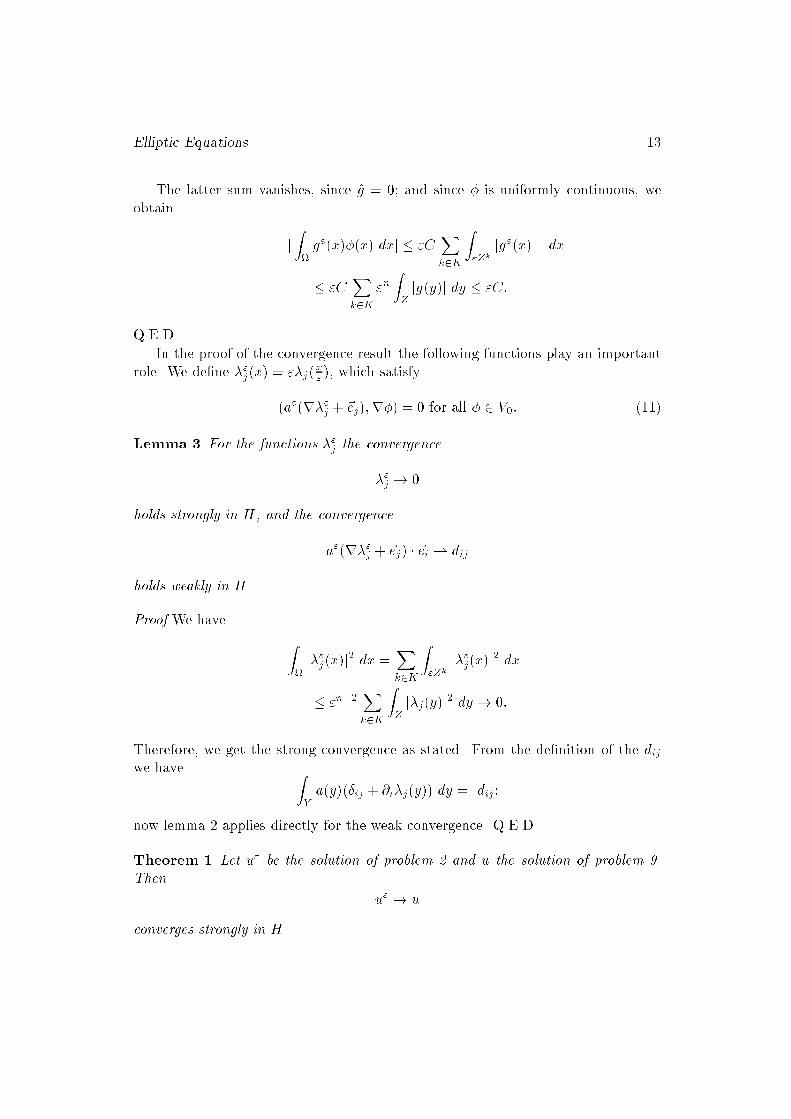
Elliptic Equations 13The latter sum vanishes, since g = 0; and since � is uniformly continuous, weobtain j Z g"(x)�(x) dxj � "C Xk2K Z"Zk jg"(x) j dx� "C Xk2K "n ZZ jg(y)j dy � "C:Q.E.D.In the proof of the convergence result the following functions play an importantrole. We de�ne �"j(x) = "�j(x" ), which satisfy(a"(r�"j + ~ej);r�) = 0 for all � 2 V0: (11)Lemma 3 For the functions �"j the convergence�"j ! 0holds strongly in H, and the convergencea"(r�"j + ~ej) � ~ei * dijholds weakly in H.Proof We have Z j�"j(x)j2 dx = Xk2K Z"Zk j�"j(x)j2 dx� "n+2 Xk2K ZZ j�j(y)j2 dy ! 0:Therefore, we get the strong convergence as stated. From the de�nition of the dijwe have ZY a(y)(�ij + @i�j(y)) dy = dij ;now lemma 2 applies directly for the weak convergence. Q.E.D.Theorem 1 Let u" be the solution of problem 2 and u the solution of problem 9.Then u" ! uconverges strongly in H.

14 HomogenizationProof Since problem 9 has a unique solution u, it su�ces to show that each sequencetaken from fu" : " > 0g has a subsequence that converges to u. For simplicity ofnotation we drop subscripts of " indicating subsequences. We may assume that u" *� weakly in V and hence u" ! � strongly in H ; furthermore, we have a"@iu" * �iweakly in H , all this at least for a subsequence. Let � 2 D be arbitrarily chosen;then we get from equation 10 in the limitXi (�i; @i�) = (f; �): (12)Using �"i� as a test function in equation 10 gives(a"ru"; �r�"i + �"ir�) = (f; �"i�);and using u"� as a test function in equation 11 gives(a"(r�"i + ~ei); �ru" + u"r�) = 0:Subtracting the last two equations yields(a"@iu"; �) + (a"(r�"i + ~ei); u"r�)� (a"ru"; �"ir�) + (f; �"i�) = 0:We get for the �rst of these terms(a"@iu"; �)! (�i; �);for the second term we knowXj (a"(@j�"i + �ij); u"@j�)!Xj (dji; �@j�)from lemma 3, and the third and fourth term tend to zero. Therefore we have inthe limit (�i; �) +Xj (dji; �@j�) = 0or after integration by parts (�i; �) =Xj (dji@j�; �);and since � was arbitrary (�i; @i�) =Xj (dji@j�; @i�):Together with equation 12 and proposition 2 this givesXi;j (dij@j�; @i�) = (f; �);which is the weak form the di�erential equation 9, since D is dense in V0; i.e., wehave shown � = u. Q.E.D.Remark: There are also estimates for u" � u available, see, e.g., [14] p. 111.

Elliptic Equations 152.6 Non-Scalar Coe�cientsHere we treat anisotropic media, i.e., we allow that the coe�cients of the originalproblem are non-scalar. We study the family of boundary value problems( r � (A"ru"(x)) + f(x) = 0; x 2 ;u(x) = uD(x); x 2 @: (13)Analogously to section 2 we assume that A" is a (not necessarily symmetric) tensorof the form A"(x) = A(x" )where A(y) is a tensor-valued function on Z for which jA(y)j (j:j being any norm)is bounded and A(y) is positive de�nite, both uniformly in y 2 Z. We go throughthe same formal asymtotic analysis as in section 2.3. For j = 1; : : : ; n we de�necell-problems for functions �j(x; y) that solvery � (A(y)ry�j(y)) = �ry � (A(y)~ej) for y 2 Z; (14)the weak form of which is(A(r�j + ~ej);r�)Z = 0 for all Z-periodic �: (15)Using these functions we now get the coe�cients fromdij = (A(r�j + ~ej); ~ei)Z :In this way one gets in the same formal way as before a homogenization result.Proposition 4 Under the assumptions of this section the homogenization of prob-lem 2 is 9 with the tensor D = (dij)i;j.This statement can also be made rigorous.Theorem 2 Under the assumptions of this section let u" be the solution of problem13 and u the solution of problem 9. Thenu" ! uconverges strongly in H.We have to modify the proof of theorem 1 in the following way. Instead of thefunctions �j we now use ��j(y) which are de�ned as solutions of the adjoint cell-problem ry � (A�(y)ry��j(y)) = �ry � (A�(y)~ej) for y 2 Z; (16)

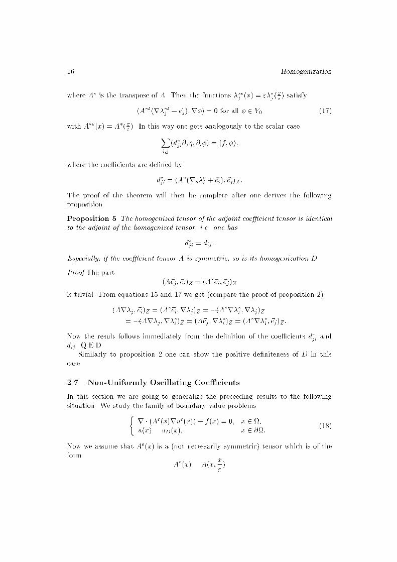
16 Homogenizationwhere A� is the transpose of A. Then the functions ��"j (x) = "��j (x" ) satisfy(A�"(r��"j + ~ej);r�) = 0 for all � 2 V0 (17)with A�"(x) = A�(x" ). In this way one gets analogously to the scalar caseXi;j (d�ji@j�; @i�) = (f; �);where the coe�cients are de�ned byd�ji = (A�(ry��i + ~ei); ~ej)Z :The proof of the theorem will then be complete after one derives the followingproposition.Proposition 5 The homogenized tensor of the adjoint coe�cient tensor is identicalto the adjoint of the homogenized tensor, i.e. one hasd�ji = dij :Especially, if the coe�cient tensor A is symmetric, so is its homogenization D.Proof The part (A~ej ; ~ei)Z = (A�~ei; ~ej)Zis trivial. From equations 15 and 17 we get (compare the proof of proposition 2)(Ar�j; ~ei)Z = (A�~ei;r�j)Z = �(A�r��i ;r�j)Z= �(Ar�j ;r��i )Z = (A~ej ;r��i )Z = (A�r��i ; ~ej)Z :Now the result follows immediately from the de�nition of the coe�cients d�ji anddij . Q.E.D.Similarly to proposition 2 one can show the positive de�niteness of D in thiscase.2.7 Non-Uniformly Oscillating Coe�cientsIn this section we are going to generalize the preceeding results to the followingsituation. We study the family of boundary value problems( r � (A"(x)ru"(x)) + f(x) = 0; x 2 ;u(x) = uD(x); x 2 @: (18)Now we assume that A"(x) is a (not necessarily symmetric) tensor which is of theform A"(x) = A(x; x" )

Elliptic Equations 17where A(x; y) depends smoothly on its �rst argument x and is Z-periodic withrespect to y. Further we make the assumption that jA(x; y)j (j:j being any norm) isbounded and A(x; y) is positive de�nite, both uniformly in x 2 . We go throughthe same formal asymtotic analysis as in section 2.3. The di�erence is that now wehave to solve a cell-problem for each point x 2 , i.e., for j = 1; : : : ; n we determinefunctions �j(x; y) that solve the cell-problemry � (A(x; y)ry�j(x; y)) = �ry � (A(x; y)~ej) for y 2 Z; (19)the weak form of which is(A(x; :)(r�j(x; :) + ~ej);r�(:))Z = 0 for all Z-periodic �: (20)Using these functions we now get the coe�cients fromdij(x) = (A(x; :)(r�j(x; :) + ~ej); ~ei)Z :As before one gets a homogenization result.Proposition 6 Under the assumptions of this section the homogenization of prob-lem 2 is 9 with the tensor function D(x) = (dij(x))i;j.This statement can also be made rigorous.Theorem 3 Under the assumptions of this section let u" be the solution of problem13 and u the solution of problem 9. Thenu" ! uconverges strongly in H.The general case is di�erent in that one no longer gets the relation 17. The proofin this case can be found in the book [17].2.8 Non-Uniformly Periodic MediaUsing the results of section 2.6 it is easy to generalize the homogenization process toproblems in which the underlying geometry is not strictly periodic. Of course, we donot make the attempt to treat absolutely arbitrary problems. Therefore, we restrictourselves in that we consider problems for which the geometry is a di�eomorphicimage of a periodic structure. We make the following assumption. Let a family ofdi�eomorphisms " : Rn ! Rn with " > 0 be de�ned such that(x) = lim"!0 "( ")�1(x) for x 2 is a di�eomorphisms from onto a domain ~ = (); we make the additionalassumption that the mapping ( ")�1 � 1" tends to 0 uniformly on . A natural

18 Homogenizationexample is "(y) = �1("y) with a given di�eomorphism ; but also any "(y) =�1("y) + o("2) would do. Now we study a boundary value problem of the form 2with a coe�cient a"(x) = a(( ")�1(x)) for all x 2 where a is a continuous Z-periodic function a : Rn ! R.Remark The previous situation of section 2 is a special case of this more generalsetting if one uses "(y) = "y for y 2 Rn. Further, it is only for simplicity ofnotations that here we consider a di�erential equation with a scalar coe�cient.The idea is to transform the problem onto the domain ~ using the mapping .To this end we need the tensor functions B(z) = (bij(z))i;j withbij(z) =Xk @zi@xk (z) @zj@xk (z)and ~A"(z) = a"(�1(z)) j@x@z (z)j B(z)where j@x@z (z)j is the functional determinant of the mapping �1 : ~! . Further,we need ~f(z) = f(�1(z)) j@x@z (z)j and ~u(z) = u(�1(z)):Lemma 4 Under the assumtions of this section problem 2 is equivalent to( rz � ( ~A"(z)rz ~u"(z)) + ~f(z) = 0; z 2 ~;~u"(z) = ~u(z); z 2 @ ~:ProofWe start from the weak form of 2, namely equation 10. According to the chainrule we have rx = rz � @z@xwhere @z@x is the Jacobian of the mapping . Therefore, we get(a"rxu";rx�) = Z a"(x)rxu"(x) � rx�(x) dx= Z~ a"(�1(z))B(z)rzu"(z) � rz�(z) j@x@z (z)j dz= ( ~A"rz ~u";rz ~�)~:Similarly we have (f; �) = (j@x@z j f; ~�)~ = ( ~f; ~�)~:Therefore, equation 10 has been transformed to( ~A"rz ~u";rz ~�)~ = ( ~f; ~�)~:

Elliptic Equations 19This is the weak form of the di�erential equation stated in the lemma, and one getsthe conclusion. Q.E.D.Instead of homogenizing problem 2 directly we now treat the boundary valueproblem of lemma 4.Lemma 5 The family of tensor functions ~A" satis�es the assumptions of section2.6, namely with the tensor function~A(z; y) = a(y) j@x@z (z)j B(z);de�ned on ~�Rn, one hasZ~ j ~A"(z)� ~A(z; z" )j dz ! 0for "! 0.Proof One gets for the integral in questionZ~ ja(1""( ")�1(�1(z)))� a(z" )j j@x@z j jB(z)j dzwhich tends to zero due to the uniform convergence of ( ")�1�1 � 1" id ! 0 andthe continuity of the function a. Q.E.D.In order to use these results and to homogenize the original problem we needthe following notations. Let ~(z) = (~sij(z))i;j be the homogenization of the tensorfamily ~A"(z) in the sense of section 2.6 and let (x) = (dij(x))i;j have the coe�cientsdij(x) =Xk;l ~sij((x)) @xk@zj (x) @xl@zi (x) j@z@x(x)j:Proposition 7 Under the assumtions of this section the homogenization of problem2 is problem 9.Proof In the same way as in lemma 4 one proves that the di�erential equationr � (~r~u) = ~f on ~transforms back onto such that one gets the boundary value problem 9. Q.E.D.2.9 Nonlinear ProblemsWe are not going to treat the details of the mathematical analysis for nonlinearproblems. The basic approach for the formal derivation of the homogenized problemsis to linearize nonlinear functions whenever they occur, e.g. to writef(u"(x)) = f(u0(x; y) + "u1(x; y) + : : :) = f(u0(x; y)) + "u1(x; y)f 0(u0(x; y)) + : : : :

20 HomogenizationFor rigorous convergence proofs the estimates needed require careful treatment. Ex-amples are given in [17] section 16 and in [14] section 5.1. A nonlinear problem ofspecial interest for ow through porous media is the dam problem. The question ofhomogenization in this case is treated in [34] and [35] [81].

Media with Obstacles 213 Media with ObstaclesIn this section we assume that the medium in which we study di�usion processeshas a periodic arrangement of obstacles. The formal description of this geometrygoes along the following lines.3.1 Solid ObstaclesWe assume that in the standard periodicity cell Z there is a standard obstacleX �� Z with smooth boundary �. The remainder is denoted by Y = Z n X .We assume that this standard geometry is repeated periodically all over Rn. Thegeometric structure within the �xed domain is obtained by intersecting the "-multiple of this periodic geometry with . The result is denoted by" = \ ("Y ) and �" = \ ("�):In order to avoid too many technical di�culties we assume that @\"� = ;. In thissituation we want to study a di�usion process that takes place only in the domainleft by the obstacles, namely in ". A simple model is the following boundary valueproblem. 8><>: r � (a"(x)ru"(x)) + f(x) = 0; x 2 ";~� � a"(x)ru"(x) = 0; x 2 �";u(x) = uD; x 2 @: (21)For simplicity, we assume that a"(x) = a(x" )with a Z-periodic function a : Y ! R. The zero ux condition on �" is used to modelthe obstacles as impermeable. Problem 21 can be looked at as a generalization of thesituation from section 2. In order to do this one has to introduce the characteristicfunction of Y , namely �(x) = ( 1; x 2 Y;0; x 2 X;and to de�ne �"(x) = �(x" ). Then one gets as the weak form of 21 the equation(�"a"ru";r�) = (f; �) for all � 2 V0; (22)which has the same formal structure as we had in equation 10. The well-posedness ofthe "-problem follows from standard analysis. Therefore, the same analysis appliesas in section 2, the di�erence being that now the cell-problems are, written in strongform, to determine Z-periodic functions �j(y) which satisfyry � (a(y)r�j(y)) = �ry � (a(y)~ej); y 2 Y;~� � ry�j(y) = �~� � ~ej ; y 2 �; (23)

22 Homogenizationand in weak form (�ar(�j + ~ej);r�)Z = 0 for all Z-periodic �:Remark In the case that a is constant on Y , the di�erential equation for �j simpli�esto ��j(y) = 0 for y 2 Y:In any case, the tensor D = (dij)i;j is de�ned bydij = (a(r�j + ~ej); ~ei)Yanalogously to section 2. In this way one gets the following result.Proposition 8 The homogenization of problem 21 is problem 9.All the rest remains almost litteraly the same as before. For the convergence proofthere is a detail to be treated carefully, namely the fact that now the functions u"are de�ned only on ", i.e., on "-dependent domains. Before one can go through thesame proof as before, one has to extend these functions into all . This is done bymeans of the following lemma.Lemma 6 (a) If a function u 2 H1;2(Y ) is given on Y there is an extension ~u intoX, and thus onto all Z, such thatk~ukH1;2(Z) � CkukH1;2(Y )(b) A function u" 2 H1;2(") can be extended to a function ~u" into all suchthat k~u"k2H1;2() � Cku"k2H1;2(")Proof: See also [33]. (a) According to our general assumption the data of the problemare su�ciently smooth. Therefore, we can �nd a neighborhood U of the interface �such that the �eld of normal vectors ~� on � allows to construct a parametrizationof U . Then we extend the function u from Y into all U by re ection at the interface�, and further into all X in any smooth manner. This procedure gives us a functionu� in all Z. We denote the average of u� over Y bym = 1jY j ZY u� dy:Now we assume that is a smooth function on Z with compact support in theinterior of X such that 1� is identically 1 on U . Then we de�ne the extension by~u = (1� )(u� �m) +m:

Media with Obstacles 23Obviously ~u is identical to u on Y . Its gradient isr~u = (u� �m)r(1� ) + (1� )ru�Therefore we get k~uk2H1;2(Z) = kuk2H1;2(Y ) + k~uk2H1;2(X)with the estimate k~uk2H1;2(X) = ZX(j ~u j2 + j r~u j2) dy:The inequality ZX j ~u j2 dy � C ZY j u j2 dyis obvious. On the other hand we haveZX j r~u j2 dy � kr(1� )kL1 ZX j u� �m j2 dy + k1� kL1 ZU j ru� j2 dy:From this we get the conclusion of the �rst part of the lemma.(b) This is a simple consequence of (a) obtained by scaling and summation.Q.E.D.Using this extension lemma one gets the following result that is essential for theconvergence proof.Lemma 7 There is an extension ~u" of the function u" into all such thatk~u"kV � Cindependently of ".Proof In the same way as in section 2 one �rst shows that the norms ku"kH1(")are uniformly bounded. Then one applies the previous lemma and gets the result.Q.E.D.Now we are ready to derive the convergence theorem.Theorem 4 Let u" be the solution of problem 21 and u the solution of problem 8,then u" ! uconverges strongly in H.Proof The proof is litteraly the same as for theorem 1. Q.E.D.What makes this problem relatively simple is the fact that we have imposedhomogeneous Neumann boundary conditions on the surfaces �" of the obstacles.The nonhomogeneous case is treated in [32].

24 Homogenization3.2 Thin ObstaclesThe situation becomes di�erent from what we have in the previous section if theobstacles are no longer "full" n-dimensional sets, but have lower dimension, say areof the form of a (n � 1)-dimensional hyper-surface. One assumes that the obstacle� �� Z is the di�eomorphic image of a (n�1)-dimensional bounded domain. Thenone studies the same boundary value problem as in problem 21 where one now hasto consider the zero ux condition on both "sides" of �". The mathematical analysisof this situation is given in [8].3.3 Non-Uniformly Periodic ObstaclesIt is natural to combine the techniques of section 2.8 with those of section 3.1. Wechose a family of di�eomorphisms " as in 2.8. Further, we assume that there is astandard obstacle Y with boundary � given and repeated periodically in Rn. Nowthe geometry within the domain is given by" = \ "(Y ) and �" = \ "(�):The boundary value problem that we are interested in is the same as problem 21,where in this case the coe�cient function isa"(x) = a(( ")�1(x)) for all x 2 ";and a is a periodic function a : Y ! R. In exactly the same way as in section 2.8one can transform this problem onto ~. Thus we get the following result.Proposition 9 Under the assumtions of this section the homogenization of problem21 is problem 9.

Parabolic Equations 254 Parabolic EquationsIn the foregoing analysis we have seen that the di�erential equations may changetheir character in the process of homogenization. E.g., an equation with a scalarcoe�cient can become anisotropic in the sense that its coe�cient is changed into atensor. When we go over to parabolic equations and treat time dependent problemswe will encounter other e�ects with change of type. Of course, if we consideredparabolic equations in the same way as we studied elliptic equations, namely just byintroducing a term with a time derivarive, in principle nothing new would come up.A term of the form @tu could formally be dealt with as another inhomogeneity, i.e.similarly to a source term f . New aspects come into play, if we allow more complexmodels on the micro-scale.4.1 Fractured MediaHere we use a con�guration on the micro-scale which is di�erent from what we had insection 3.1 in that we now allow ow to take place in the interior of the aggregates.We assume that in the standard periodicity cell Z there is a standard aggregateX �� Z with smooth boundary � the remainder of which is denoted by Y = Z nX .As before, we assume that this standard geometry is repeated periodically all overRn. The geometric structure within the �xed domain is obtained by intersectingthe "-multiple of this periodic geometry with . The result is�" = \ ("X) , " = \ ("Y ) and �" = \ ("�):First we study a di�usion process in which two scales for the di�usivity occur.We start from the following initial boundary value problem.8>>>>>>>>>><>>>>>>>>>>: @tv"(t; x) = r � (a"(x)rv"(t; x)); t > 0; x 2 ";@tw"(t; x) = "2r � (b"(x)rw"(t; x)); t > 0; x 2 �";a"(x)~� � rv"(t; x) = "2b"(x)~� � rw"(t; x); t > 0; x 2 �";"d"(x)b"(x)~� � rw"(t; x) = v"(t; x)� cw"(t; x); t > 0; x 2 �";v"(t; x) = vD(t; x); t > 0; x 2 @;v"(t; x) = vI(x); t = 0; x 2 ;w"(t; x) = wI(x); t = 0; x 2 : (24)We make the assumption that the coe�cients a"k and d" are oscillating, i.e., that wehave a"k(x) = ak(x" ) and d"(x) = d(x" );where the functions ak and d are Z-periodic. The parameter d has been introducedin order to allow di�erent types of models, namely for d = 0 one getsv"(x) = cw"(x)

26 Homogenizationon the interface �", whereas for d > 0 one has a boundary condition of Robin type.In any case we assume c > 0. The formal asymptotics is not exactly the same asin section 2 since we have to take care of the factors " and "2 which appear in themodel. The starting point is as usual the ansatz that the unknowns can be writtenas a power series in the formv"(t; x) = v0(t; x; y) + "v1(t; x; y) + "2v2(t; x; y) : : :and w"(t; x) = w0(t; x; y) + "w1(t; x; y) + "2w2(t; x; y) : : :with the usual assumption of Z-periodicity of the coe�cient functions. For simplicityof notation we drop the variable t in the following. The di�erential equation for v"in " gives "0@tv0(x; y) + "1 : : := "�2ry � (a(y)ryv0(x; y))+"�1(ry � (a(y)ryv1(x; y)) +ry � (a(y)rxv0(x; y))+a(y)rx � ryv0(x; y)))+"0(ry � (a(y)ryv2(x; y) + a(y)rxv1(x; y))+a(y)rx � ryv1(x; y) + a(y)rx � rxv0(x; y))+"1(: : :) + : : : ; y 2 Y: (25)The di�erential equation for w" in �" gives"0@tw0(x; y) + "1 : : : = "0ry � (b(y)ryw0(x; y)) + "1 : : : ; y 2 X (26)The two conditions on the interface �" yield"�1a(y)~� � ryv0(x)+"0a(y)~� � (ryv1(x) +rxv0(x))+"1(a(y)~� � (ryv2(x) +rxv1(x)))+"2 : : : = "1b(y)~� � ryw0(x; y) + "2 : : : ; y 2 � (27)and "0d(y)b(y)~� � ryw0(x; y) + "1 : : := "0(v0(x; y)� cw0(x; y)) + "1 : : : ; y 2 �: (28)Now we have to compare the coe�cients of the di�erent "-powers in these equations.The term with "�2 in equation 25 givesry � (a(y)ryv0(x; y)) = 0 for y 2 Y:

Parabolic Equations 27Since v0(x; y) is Z-periodic in the variable y, we obtain that v0(x; y) = v0(x) is afunction of x alone independently of y. Using this, the term with "�1 in equation25 gives ry � (a(y)ryv1(x; y)) = �ry � (a(y)rxv0(x)) for y 2 Y:One expresses the function v1(x; y) in terms of the function v0(x) in the same wayas in section 2.5. Using the functions �j(y) from 23 with a instead of a we getv1(x; y) = nXj=1�j(y)@xjv0(x) + v1(x);where v1(x) is independent of y. We proceed further and look at the term with "0in equation 25. We get@tv0(x; y) = ry � (a(y)ryv2(x; y) + a(y)rxv1(x; y))+a(y)rx � ryv1(x; y) + a(y)rx � rxv0(x) for y 2 Y:We integrate this identity over Y and obtainjY j@tv0(x)= ZY ry � (a(y)ryv2(x; y) + a(y)rxv1(x; y)) dy+ ZY a(y)rx � ryv1(x; y)dy+ ZY a(y)dy �xv0(x); (29)We integrate the �rst integral on the right side by parts and getZY ry � (a(y)ryv2(x; y) + a(y)rxv1(x; y)) dy= Z@Y a(y)~� � (ryv2(x; y) +rxv1(x; y)) d�(y):We have @Y = @Z + �; the boundary integral over @Z vanishes because of theZ-periodicity of the functions v2(x; y) and v1(x; y). For the integral over � we havea look at the term "1 in 27 and getZ� a(y)~� � (ryv2(x; y) +rxv1(x; y)) d�(y) = Z� b(y)~� � ryw0(x; y) d�(y):For the second term in equation 29 we get in the well known wayrx � ryv1(x; y) = nXi;j=1@yi�(y)@xixjv0(x):

28 HomogenizationTherefore, we obtain from equation 29jY j@tv0(x; y)� Z� b(y)~� � ryw0(x; y) d�(y)= nXi;j=1 ZY a(y)@yi�(y)dy @xixv0(x) + ZY a(y)dy �xv0(x):The term with "0 in equation 26 yields@tw0(x; y) = ry � (b(y)ryw0(x; y)); y 2 X;and the term with "1 in equation 28 givesd(y)b(y)~� � ryw0(x; y) = v0(x)� cw0(x; y); y 2 �:In this way we have shown the following result. For clari�cation we write the timevariable t again.Proposition 10 The homogenization of the initial boundary value problem 24 is8>>>>>>>>>><>>>>>>>>>>: jY j@tv(t; x) + S(t; x) = r � (Drv(t; x)); t > 0; x 2 ;S(t; x) = � R� b(y)~� � ryw(t; x; y) d�(y); t > 0; x 2 ;@tw(t; x; y) = ry � (b(y)ryw(t; x; y)); t > 0; x 2 ; y 2 X;d(y)b(y)~� � ryw(t; x; y) = v(t; x)� cw(t; x; y); t > 0; x 2 ; y 2 �;v(t; x) = vD(t; x); t > 0; x 2 @;v(t; x) = vI(x); t = 0; x 2 ;w(t; x) = wI(x); t = 0; x 2 : (30)The homogenized problem can be rewritten in several di�erent ways. We use theaverage �w(t; x) = 1jX j ZX w(t; x; y)dy:Proposition 11 The source/sink term S(t; x) can be represented asS(t; x) = ZX ry � (b(y)ryw(t; x; y)) dy = ZX @tw(t; x; y) dy = jX j@t �w(t; x):If the function r : [0;1)�X ! R solves the initial boundary value problem8><>: @tr(t; y) = ry � (b(y)ryr(t; y)); t > 0; y 2 X;d(y)b(y)~� � ryr(t; y) = �cr(t; y); t > 0; y 2 �;r(t; y) = 1; t = 0; y 2 X (31)then one has w(t; x; y) = (wI(x)� 1cvI(x))r(t; y)+1c (v(t; x)� Z t0 r(t� s; y)@tv(s; x) ds);

Parabolic Equations 29and with ~�(t) = ZX r(t; y) dyone can writeS(t; x) = �(wI(x)� 1cvI(x)) ddt�(t)� 1c Z t0 ddt~�(t� s)@tv(s; x) ds:Proof: The representation of S as a volume integral is obtained using integration byparts, where now ~� is the inner normal on @X . Let ~w be the expression given in theproposition for w. Then we get@t ~w(t; x; y) = (wI(x)� 1cvI(x))@tr(t; y)+1c (@tv(t; x)� r(0; y)@tv(t; x)� Z t0 @tr(t� s; y)@tv(s; x) ds)This is equal to ry � (b(y)ryw(t; x; y)) = (wI(x)� 1cvI(x))ry � (bryr(t; y))�1c Z t0 ry � (bryr(t� s; y))@tv(s; x) ds:Therefore ~w sati�es the di�erential equation required. Moreover, we haved(y)b(y)~� � ryw(t; x; y) == (wI(x)� 1cvI(x))d(y)b(y)~� � ryr(t; y)�1c Z t0 d(y)b(y)~� � ryr(t� s; y)@tv(s; x) ds:This equals to v(t; x)� cw(t; x; y) = v(t; x)� (cwI(x)� vI(x))r(t; y)�v(t; x) + Z t0 r(t� s; y)@tv(s; x) ds:Therefore, ~w also sati�es the proper boundary condition. The initial condition~w(0; y) = wI(x) is trivial; therefore, we get ~w = w. The �nal representation of S isjust a matter of di�erentiation with respect to t and integration over X . Q.E.D.Proposition 12 If X is a ball of radius R and b = a is a constant, then the kernel~� is given by ~�(t) = jX j 6�2 1Xk=1 1k2 e��2k2at

30 HomogenizationProof: The cell function r in this case isr(t; y) = 2� 1Xk=1 (�1)k�1k e��2k2at sin(�k jyjR ):The kernel ~� is obtained by integration over X . Q.E.D.Corollary 1 If the initial data are zero, one gets the problem8>>>>><>>>>>: jY j@tv(x) + S(x) = r � (Drv(x)); t > 0; x 2 ;S(x) = �1c R t0 ddt~�(t� s)@tv(s; x) ds; t > 0; x 2 ;v(t; x) = vD(t; x); t > 0; x 2 @;v(t; x) = 0; t = 0; x 2 ;w(t; x) = 0; t = 0; x 2 : (32)A problem of this type with d = 0 was dealt with in [91]; a convergence proof fora problem with a lower order term was given in [6], see also chapter 2 of [7]. In thenext section we give another convergence proof. The well-posedness of the initialboundary value problem of corollary 1 was studied independently in [56].4.2 Convergence ProofThe existence and uniqueness of the solutions of the "-problems is standard and nottreated here in detail. We introduce the follwoing shorthand notations:Q = [0; T ]� ; U = Q�X; Q" = [0; T ]� "; R" = [0; T ]��":In order to simplify the calculations, we treat only the following special case. Weassume c = 1, d = 0, vD = 0, and a, b to be constant. In this special case the weakform of problem 24 is(@tv"; ')" + (@tw"; )�" + a(rv";r')" + "2b(rw";r )�" = 0 (33)for all test functions ' 2 H1(") with 'j@ = 0, 2 H1(�") and 'j�" = j�" (inother words, we use functions from H10() which we denote by ' on " and by on�"). First of all we give estimates of the solutions v" and w" that are independentof ".Proposition 13 For the solution of the micro-model problem 24 the estimateskv"kL2(0;T ;H1(")) � C; "krw"kL2(0;T ;L2(�")) � C;k@tv"kL1(0;T ;L2(")) � C; k@tw"kL1(0;T ;L2(�")) � C;and kr@tv"kL2(0;T ;L2(")) � C; "kr@tw"kL2(0;T ;L2(�")) � Chold independently of ".

Parabolic Equations 31Proof: Plugging ' = v" and = w" into equation 33 we get(@tv"; v")" + (@tw"; w")�" + a(rv";rv")" + "2b(rw";rw")�" = 0:We integrate this over [0; t] and obtain12(kv"(t)k" + kw"(t)k�")+ Z t0 �a(rv";rv")" + "2b(rw";rw")�"� d� = 12(kvIk" + kwIk�"):Hence we get the �rst two estimates. Now we di�erentiate equation 33 and get(@ttv"; ')" + (@ttw"; )�" + a(@trv";r')" + "2b(@trw";r )�" = 0:Here we use the test functions ' = @tv" and = @tw" and get by integration overtime12(k@tv"(t)k" + k@tw"(t)k�")+ Z t0 �a(@trv"; @trv")" + "2b(@trw"; @trw")�"� d� = 12(kvIk" + kwIk�"):where vI = r � a(rvI) and wI = "2r � b(rwI). In this way we get all the remainingestimates. Q.E.D.From now on we identify v" with its extension according to lemma 6; let ~�" = rv"(extended by "2rw" in the interior of �"). Note that the extension lemma from [33]pp. 593-597 implies that r � ~�" is uniformly bounded in L2(Q). We we also identifyw" with its H1-extension de�ned by w" = v" on ". Then we getProposition 14 There is a subsequence such thatv" * v� weakly in L2(0; T ;H1());v" * v� weak� in L1(Q);@tv" * @tv� weakly in L2(Q);v" ! v� strongly in L2(0; T ;L2());~�" * ~�� weakly in (L2(Q))nwith some v� and ~��, such that r � ~�� is bounded in L2(Q).Proof: This follows from proposition 13. Q.E.D.In order to prove the convergence result, we use the notion of two-scale conver-gence which was introduced in [75] and developed further in [3], see also [4]. Theidea behind this concept was used in [6].

32 HomogenizationDe�nition 1 The sequence fw"g � L2(Q) is said to two-scale converge to a limitw 2 L2(Q � Z) i� for any � 2 C1(Q;C1per(Z)) ("per" denotes Z-periodicity) onehas lim"!0 ZQw"(t; x)�(t; x; x" ) dx dt = ZQ ZZ w(t; x; y)�(t; x; y) dy dx dt:Lemma 8 From each bounded sequence in L2(Q) one can extract a subsequencewhich two-scale converges to a limit w 2 L2(Q� Z).Proof: See [75]. Q.E.D.Lemma 9 Let w" and "rw" be bounded sequences in L2(Q). Then there existsa function w 2 L2(Q;H1per(Z)) and a subsequence such that both w" and "rw"two-scale converge to w and ryw, resp.Proof: See [3] and [75]. Q.E.D.Proposition 15 There is a subsequence such thatw" ! w�@tw" ! @tw�"rw" ! ryw�in the two-scale sense with some w� 2 L2(Q;H1per(Z)) \H1(0; T ;L2(� Z)).Proof: This follows from the estimates of proposition 13 and lemma 9. Q.E.D.Proposition 16 The function w� de�ned in proposition 15 satis�esw�jt=0 = wI a.e. on �X:Proof: Let ' 2 C10 () and ! 2 C10 (0; T ) with !(T ) = 0. Furthermore, let � 2C10 (X). We extend � by zero to Z nX and Z-periodically to Rn. We de�ne �" by�"(x) = �(x" ). Then we have(@tw"; '�"!)R" = �(wI ; '�")�" !(0)� (w"; '�"@t!)R":Passing to the limit yieldsZU @tw�� dy ' dx ! dt = � Z ZX wjI� dy ' dx� ZU w�� dy ' dx @t! dtand thus the equality to be proved. Q.E.D.Proposition 17 For the subsequences in propositions 14 and 15 the relationsv� = w�hold on Q� �.

Parabolic Equations 33Proof: Let ~� 2 C1(X), extend it Z-periodically and de�ne ~�"(x) = ~�(x" ). Thenwith 2 C10 () and ! 2 C10 (0; T ) we get0 = Z T0 "(v" � w"; ~� � ~�" !)�" dt = Z T0 "(r � (~�" (v" � w") ); !)�" dt= Z T0 "(r � ~�" (v" � w"); )�" ! dt+ Z T0 "(~�" � r(v" � w"); )�" ! dt +O(")Now we determine the limits of these two terms separately. We havelim"!0 Z T0 "(r � ~�" (v" � w"); ��") ! dt = ZU ry � ~� (v� � w�) dy dx ! dtand lim"!0 Z T0 "(~�" � r(v" � w"); ��") ! dt = ZU ~� � ry(v� � w�) dy dx ! dt:Therefore, we concludeZU ry � (~� (v� � w�)) dy dx ! dt = 0and hence Z� ~� � ~� (v� � w�) d�(y) = 0:Since ~� was arbitrary, we have v� = w� on �. Q.E.D.Proposition 18 The function w� from proposition 15 satis�es(@tw�; �)U + b(ryw�;ry�)U = 0 8� 2 L2(Q;H1(X)):Proof: We choose � 2 C10 (Q;C1per(Z)) such that � = 0 on Y . We de�ne �"(t; x) =�(t; x; x" ). Then we get by integration over (0; T )(@tw"; �")R" + "2b(rw";r�")R" = (@tw"; �")Q + "2b(rw";r�")Q = 0:Since (@tw"; �")Q ! (@tw�; �)Uand "2(rw";r�")Q ! (ryw�;ry�)U ;we get the result. Q.E.D.Proposition 19 The function ~�� from proposition 14 satis�es~�� = Drv�: (34)

34 HomogenizationProof: We introduce the functions �j(y) = �j(y) + yj which we identify with theirextensions according to lemma 6 (a). Let �"j(x) = �j(x" ), ~�j = ry�j , and ~�"j(x) =~�j(x" ). It is known (see, e.g., [33] or [54]) that�"j * ��j weakly in H1()r�"j * ~ej weakly in (L2())n~�"j * D~ej weakly in (L2())nfor some ��j which satis�es r��j = ~ej . The extension lemma from [33] impliesr � ~�"j = 0 in . Let ' 2 C10 () and ! 2 C10 (0; T ). Then we get(~�"j ;rv"'!)Q + (~�"j ; v"r'!)Q = 0:Passing to the limit "! 0 and by using the "div-curl"-lemma from [73] we get(~�"j ;rv"'!)Q = (r�"j ; ~�"'!)Q ! (~ej ; ~��'!)Qand (~�"j ; v"r'!)Q ! (D~ej ; v�r'!)Q:Therefore, we have (��; ~ej'!)Q = (Drv�; ~ej'!)Q:Since ', and ! were arbitrary, we get the result. Q.E.D.Proposition 20 For the the limit of the subsequence in proposition 14 the relation(jY j@tv� + S; ')Q+ (Drv�;r'))Q = 0 8' 2 L2(0; T ;H1()) with 'j@ = 0 (35)holds.Proof: Let ' 2 C10 (Q). Then we use ' for both test functions ' and in theequation 33 and get by integration over (0; T )(@tv"; ')Q" + (@tw"; ')R" + a(rv";r')Q" + "2b(rw";r')R" = 0Now propositions 14, 15, and 18 imply by taking the limitsjY j(@tv�; ')Q+ (@tw�; ')U + (Drv�;r')Q = 0Q.E.D.

Parabolic Equations 35Theorem 5 The limit functions ~v� and ~w� solve the macro-model problem 30. Andthe extensions of the sequences v" and w" satisfyv" * v weakly in L2(0; T ;H1())@tv" * @tv weakly in L2(Q)v" ! v strongly in C([0; T ]; L2())w" * w in the two-scale sense@tw" * @tw in the two-scale sense"rxw" * ryw in the two-scale senseProof: We have only to collect the results from propositions 16, 17 18, and 20. Theconvergence of the whole sequences follows since the limit functions are uniquelydetermined, see [56]. Q.E.D.4.3 Miscible Displacement In uenced by Mobile and ImmobileWa-terThe model that we are going to study in this section is slightly di�erent from whatwe had in the preceeding section. Now we allow also convection of a dissolvedsubstances. We use the same geometry as before and start from the following familyof problems.8>>>>>>>>>>>>>>>>>>><>>>>>>>>>>>>>>>>>>>:~u"(x) = �k"(x)rp"(x); x 2 ";r � ~u"(x) = 0; x 2 ";~� � ~u"(x) = 0; x 2 �";�@tv"(t; x)= r � (a"(x)rv"(t; x))� ~u"(x) � rv"(t; x); t > 0; x 2 ";#@tw"(t; x) = "2r � (b"(x)rw"(t; x)); t > 0; x 2 �";a"(x)~� � rv"(t; x) = "2b(x)"~� � rw"(t; x); t > 0; x 2 �";v"(t; x) = w"(t; x); t > 0; x 2 �";v"(t; x) = vD(t; x); t > 0; x 2 @;v"(t; x) = vI(x); t = 0; x 2 ";w"(t; x) = wI(x); t = 0; x 2 �": (36)The physical interpretation is that a porous medium consists of two parts: In "steady ow of water takes place according to Darcy's law. Here a solute is trans-ported and it undergoes di�usion and convection. In the second part of the medium�" the water is assumed to be at rest. The solute transport is only in uenced bydi�usion here. The important aspect is that the difussivity is orders of magnitudesmaller in �" than in ". The words used by soil physicists in this context are mobilewater in " and immobile water in �". This type of problems was studied in [52].

36 HomogenizationThe homogenized limit problem of the system 36 is the following.8>>>>>>>>>>>>>>>><>>>>>>>>>>>>>>>>: ~u(x) = �Krp(x); x 2 ;r � ~u(x) = 0; x 2 ;jY j�@tv(t; x) + S(t; x)= r � (Drv(t; x))� ~u(x) � rv(t; x); t > 0; x 2 ;S(t; x) = RX @tw(t; x; y) dy; t > 0; x 2 ;#@tw(t; x; y) = ry � (b(x)ryw(t; x; y)); t > 0; x 2 ; y 2 Xv(t; x) = w(t; x; y); t > 0; x 2 ; y 2 �;v(t; x) = vD(t; x); t > 0; x 2 @;v(t; x) = vI(x); t = 0; x 2 ;w(t; x) = wI(x); t = 0; x 2 : (37)Here the relation between k" and K is the same as between a" and D. The conver-gence proof is almost the same as in section 4.2. The paper [52] gives also numericalresults for one-dimensional in�ltration experiments that lead to break-through curves.There comparisons are also given with this system and the standard approach usedin soil science.4.4 Flow and Transport in Unsaturated Fractured MediaIn the paper [7] the problem of immiscible displacement of two liquids, such as waterand oil, in a fractured porous medium is studied. There both the micro-system isgiven and also the macro-system which can be obtained by a formal homogenizationprocedure. We do not repeat the rather complicated system of equations. Systemsof that kind have already been used in oil reservoir simulation for several years, see[37].In a certain sense the problem of unsaturated ow is a limit case of the immiscibledisplacement problem. One comes to this conclusion by considering the two uidswater and air. If one makes the assumption that the conductivity of the air is largeenough such that the air pressure is everywhere always at atmospheric pressure, onegets rid of the equation describing the air ow. Here we shortly give such a system.At the same time we couple the water ow with the transport of a solute. Aftergoing through all the formal calculations one is lead to the following system.For the water ow one has8>>>>>>>><>>>>>>>>: jY j@t� + S = �rx � ~Q ; x 2 ~Q = �K(rx + ~e) ; x 2 S = R� ~� � ~q d�(y) ; x 2 @t# = �ry � ~q ; x 2 ; y 2 Y~q = �kry ; x 2 ; y 2 Y = ; x 2 ; y 2 �

Parabolic Equations 37For the concentration of the solute one hasjY j@t(�v) + R = rx � (Drxv � v ~Q) ; x 2 R = R� ~� � ~r d�(y) ; x 2 @t(#w) = �ry � ~r ; x 2 ; y 2 Y~r = �dryw + w~q ; x 2 ; y 2 Yv = w ; x 2 ; y 2 �A system of this type was described in more detail in [51].

38 Homogenization5 Problems on the Pore Scale5.1 Derivation of Darcy's LawWe start from the following problem on the pore scale. The geometry is the sameas in section 3 8><>: "2�~u"(x) = rp"(x); x 2 ";r � ~u"(x) = 0; x 2 ";~u"(x) = 0; x 2 �": (38)The reason that one chooses the "2 to enter in this way into the problem is thatwe want to scale the velocity �eld ~u" such that it has a weak limit ~u. Here we givethe formal asymptotics of this problem. We are also going to sketch the proof; forthe details we refer to the book [86] and the paper [90]. As usual we start from theassumption that there is a power series of the unknown functions of the form~u"(x) = ~u0(x; y) + "~u1(x; y) + "2~u2(x; y) : : :and p"(x) = p0(x; y) + "p1(x; y) + "2p2(x; y) : : :with Z-periodicity of the coe�cient functions. From this one gets the followingequations "0�y~u0(x; y) + "1(: : :) + : : := "�1ryp0(x; y) + "0(ryp1(x; y) +rxp0(x; y))+"1(: : :) + : : : ; y 2 Y; (39)"�1ry � ~u0(x; y) + "0(ry � ~u1(x; y) +rx � ~u0(x; y))+"1(: : :) + : : : = 0; y 2 Y; (40)"0~u0(x; y) + "1~u1(x; y) + : : : = 0; y 2 �: (41)Comparing the coe�cients goes along the following lines. The "�1 term in equation39 gives ryp0(x; y) = 0; y 2 Y;hence p0(x; y) = p0(x) independently of y. The "0 term in equation 39 gives�y~u0(x; y) = ryp1(x; y) +rxp0(x); y 2 Yand the "�1 term in equation 40 yieldsr � ~u0(x; y) = 0; y 2 Y:In the usual way one writes rxp0(x) =Xj ~ej@jp0(x):

Pore Scale Problems 39The cell-problems are now to �nd Z-periodic vector �elds ~�j(y) with components�ji(y) that solve the Stokes problems�y~�j(y) = ry�j(y)� ~ej ; y 2 Y;r � ~�j(y) = 0; y 2 Y;~�j(y) = 0; y 2 �; (42)where the functions �j(y) are the corresponding Z-periodic pressure �elds. Usingthese cell-functions we get easily~u0(x; y) = �Xj ~�j(y)@jp0(x):One de�nes the averaged vector �eld�u(x) = ZY ~u0(x; y)dyand gets for its i-th component�ui(x) = �Xj kij@xjp0(x)with kij = RY �ji(y)dy:If one introduces the tensor K = (kij)i;j , one gets for short�u(x) = �Krp0(x)which is Darcy's law. It remains to show that the velocity �eld �u is divergence free.The term with "0 in equation 40 givesry � u1(x; y) +rx � u0(x; y) = 0; y 2 YIntegrating this over Y givesrx � �u(x) = ZY r � ~u0(x; y)dy = � ZY ry � ~u1(x; y)dy= � Z@Y ~� � ~u1(x; y)d�(y) = � Z� ~� � ~u1(x; y)d�(y)� Z@Z ~� � ~u1(x; y)d�(y):The boundary integral over � is zero due to the term with "1 in equation 41, and theboundary integral over @Z is zero due to the Z-periodicity of ~u1(x; y) with respectto y. Therefore, we have shown

40 HomogenizationProposition 21 The homogenization of the Stokes problem 38 is�u(x) = �Krp(x); r � �u = 0 (43)One gets similarly to section 2 the symmetry and positive de�niteness of the tensorK.Lemma 10 The tensor K is symmetric and positive de�nite.Proof The weak form of the cell problems for the vector �elds ~�j is((~�j ; ~�))Y = (~ej ; ~�)Yfor all Z-periodic vector �elds ~� with r� ~� = 0 in Y and ~� = 0 on �, where we haveused the bilinear form ((~�; ~ ))Y =Xl;k (@l�k; @l k)Y :Thus one gets with ~�i as a test function((~�j ; ~�i))Y = (~ej ; ~�i)Y = kji:With indices j and i interchanged one gets((~�i; ~�j))Y = (~ei; ~�j)Y = kij :Since the left hand sides are equal, so are the right hand sides. Therefore, K issymmetric. If real numbers �1; : : : ; �n are given, then one has�ikij�j = �i(~ei; ~�j)Y �j = ((�i~�i; �j~�j))Y :The sum over these terms is positive, whenever one of the �i is di�erent from zero.Q.E.D.Theorem 6 Let ~u" be extended by zero to n ". Then there exists an extension~p" of the pressure p" such that~u" * ~u weakly in (L2())n~p" ! p strongly in L20()with ~u 2 (L2())n and p 2 L20() which solve the system 43.Proof: This result goes back to the paper [90]. Generalizations can be found in[1] and [70]. An explicit formula for the extension of the pressure is given in [63].Q.E.D.Let us note that the result of the previous theorem remains also valid for thecase of Navier-Stokes equations with the convergence of the pressure taking place insome appropriate functional spaces; for more details see [68].

Pore Scale Problems 415.2 Immiscible Displacement ProblemsThe result of the previous section applies to ow of a single uid in a nondeformableporous medium. For two immiscible uids the situation is more complicated, sinceone has to consider the interface between the two phases. In general this seemsto be a very di�ucult question. If one makes the assumption that the geometry ofthe interface varies only slightly from cell to cell, one can perform a perturbationanalysis similar to the single uid case. In this chapter we give an outline of an ideathat can be found in [10]. It should be pointed out that the underlying assumption isthat the ow problem with a capillary interface has a unique solution and dependscontinously on the data. The validity of this assumption may be very limited.Therefore, the result of this section has only limited applicability.We consider the following problem on the micro-scale. We look for a velocity�eld ~u" de�ned on " (that has no jump across the interface �"�) the restrictions ofwhich to "i we denote by ~u"i , and a pressure �eld p" (that may have a jump across�"�) such that 8>>>>><>>>>>: "2�i�~u"i = rp"i ; x 2 "i ; i = w; nr � ~u"i = 0; x 2 "i ; i = w; n~u"w = 0; x 2 �"s~u"i � ~� = 0 x 2 �"�; i = w; n[T "] � ~� = "�2H"~�; x 2 �"� (44)Here we have T "i = �p"i I + "2�i2S"i for i = w; n;I is the identity, S" is the stress tensor with componentss"jk = 12(@jv"k + @kv"j );and [� � �] denotes the jump across �"�. Further, H" is the mean curvature of thesurfave �"�.In the sense of distributions one gets from 44r � T " = "�2H"~���"�in ". In the special case that the uid is at rest, one hasrp"i = 0 and [�p"] = "�2H"on �"�.We introduce the spacesW" = f~u : ~u 2W1;2(") with ~u = 0 on �"g;W"0 = f~u : ~u 2 W with ~u = 0 on @gand V" = f~u : ~u 2 W with r � ~u = 0 in "g

42 Homogenizationof vector �elds on ".Furthermore, we introduce the sesquilinear formE(~u; ') = Ew(~uw; ') + En(~un; ')with Ei(~u; ') = "2�i 12Xj;k Zi(@kvj + @jvk)(@k�j + @j�k) d:The number E(~u; ~u) is the energy dissipating within the domain ".Using integration by parts one gets easily the following formula.Lemma 11 If ~u" 2 V" and ' 2 W", then one has(�"2��~u"i +rp"; ')"i= Ei(~u"i ; ')� (p"i ;r �')"i � Z�"� ~� � T "i �' d�;where the " + " and the "� " apply for i = w and i = n, respectively.From this we get the following weak form of the micro-problem.Proposition 22 A vector �eld ~u" solves the micro problem 44 i� ~u" 2 W" with~u"w � ~� = ~u"n � ~� = 0 on �"� such that there exists a pressure �eld p" 2 L2(") with( E(~u"; ')� (p";r � ')" = "�(2H"~�; ')�"� 8' 2 W"0(r � ~u"; )" = 0 8 2 L2(")The second condition ensures that ~u" is divergence free. We just mention that thisproblem can be reformulated as a minimization problem.For the aymptotic expansion we make the following assumptions.~u"(x) = "0~u0(x; y) + "1~u1(x; y) + "2 : : :p"(x) = "0p0(x; y) + "1p1(x; y) + "2 : : :�"�(x; y) = "1�0�(x; y) + "2�(x; y) + "3 : : :with y = x" and all coe�cients in the series being periodic functions of the fastvariable y. By �0�(x) we mean a surface in y-space; whereas �(x; y) denotes a vectorvalued function on �0�(x) that is parallel to the normal vector ~�0(x; y) on �0�(x). Inother words, we assume that the free boundary problem 44 is a perturbation of azero order problem. The perturbation is thought of as being of order ".First we identify the zero order problem. We get the following expansions."0�i�y~u0i (x; y) + "1 : : := "�1ryp0i (x; y) + "0(ryp1i (x; y) +rxp0i (x; y)) + "1 : : : y 2 Yi(x) (45)

Pore Scale Problems 43"�1ry � ~u0i (x; y) + "0(ry � ~u1i (x; y) +rx � ~u0i (x; y)) + "1 : : : = 0; y 2 Yi(x) (46)"0~u0w(x; y) + "1~u1w(x; y) + "2 : : : = 0; y 2 �s (47)When calculating the perturbations of the conditions on the interface �0�(x) we haveto take into account the perturbation of this interface also. We get("0~u0i (x; y) + "1 : : :) � ~� = 0; y 2 ��(x) (48)The expansion of the stress tensor isT "(x) = T 0(x; y) + "T 1(x; y) + "2 : : :with T 0jk = �p0(x; y)�jkand T 1jk = �(p1(x; y) +ryp0(x; y) � �(x; y))�jk + �(ryj~u0k(x; y) +ryk~u0j (x; y))and for the curvature we have"�2H"(x) = "0�2H0(x; y) + "1�2H1(x; y) + "2 : : :Therefore, from the "0 term of the jump condition on the interface we get[�p0(x; y)] = �2H0(x; y); y 2 ��(x) (49)From the "�1 term in equation 45 we getryp0i (x; y) = 0; y 2 Yi(x)which yields p0i (x; y) = p0i (y)From 49 we get [�p0(x)] = �2H0(x; y); y 2 �0�(x)and therefore [�p0(x)] = �2H0(x); y 2 �0�(x) (50)i.e., the interface �0�(x) has a mean curvature which is independent of the fast variabley. Hence the zero order problem is to �nd a periodic surface �0�(x) having meancurvature H0(x) which is given by equation 50.Now come to the �rst order problem. From the "0 term in 45, the "�1 term in46, the "0 terms in 47 and 48 we get8>>><>>>: �i�y~u0i (x; y) = ryp1i (x; y) +rxp0i (x); y 2 Yi(x)ry � ~u0i (x; y) = 0; y 2 Yi(x)~u0w(x; y) = 0; y 2 �s~u0i (x; y) � ~� = 0; y 2 �0�(x) (51)

44 HomogenizationIt has to be kept in mind that the velocity �eld ~u0 is continuous across the interface�0�(x), whereas the pressure �eld p1(x; :) is allowed to have a jump. The average�vi(x) = ZYi ~u0i (x; y) dythen satis�es �v0i (x) = �Xj ZYi ~u0i (x; y) dy @jp0(x) (52)which is the generalized Darcy law.5.3 Elastic Porous MediaIn soil mechanics porous media are considered to be deformable. Very often onemakes the assumtion that the soil behaves like an elastic body. Models for thisphenomenon go back to Biot [20] [21] [22]. A formal derivation of this type ofmodels was given in [29] for one-phase ow. The problem of two-phase immiscible ow was studied in [9] and [10], see also [38].5.4 ChromatographyIn chemical engineering an important e�ect is known which is called chromatogra-phy. Here certain chemical species are dissolved in a uid that is owing througha porous medium. These are not only transported by convection and di�usion butthey also penetrate into the porous matrix. If one assumed that the species underconsideration may di�use within the interior of the solid matrix one comes to modelsthat were studied theoretically in [91] and practically in [87]. A nonlinear problemof this type is investigated in [30].5.5 Semipermeable MembranesIn biology a situation is of interest in which chemical species are owing withinthe space between cells. The cells are surrounded by membranes that are partiallypermeable. If one assumes that the membranes are semipermeable, special nonlinearinterface conditions have to be formulated. One case is to use the setM � R2 de�nedby (s; q) 2M i� s � 0 and q � 0 and sq = 0:The condition to be postulated on the interfaces �" is a relation between the dif-ference s of the outer and inner contration v and w, resp., and the normal uxq.

Pore Scale Problems 45The micro-problem is the following.8>>>>>>>>>>>>>>>>>>>>>>><>>>>>>>>>>>>>>>>>>>>>>>:"2�~u"(x) = rp"(x); x 2 "r � ~u"(x) = 0; x 2 "~u(x) = ~uD; x 2 �D~� � ~u"(x) = 0; x 2 �N~u"(x) = 0; x 2 �"@tv"(t; x) = a�v"(t; x)� ~u"(x) � rv"(t; x) + f(~v"(t; x)) ; t > 0; x 2 "@tw"(t; x) = "2c�w"(t; x) + g(~w"(t; x)) ; t > 0; x 2 �"a~�" � rv"(t; x) = "2c~�" � rw"(t; x) ; t > 0; x 2 �"(v"(t; x)� w"(t; x);�"2c~�" � rw"(t; x)) 2M ; t > 0; x 2 �"v"(t; x) = vD(t; x) ; t > 0; x 2 �D~� � rv"(t; x) = 0 ; t > 0; x 2 �Nv"(t; x) = vI(x) ; t = 0; x 2 "w"(t; x) = wI(x) ; t = 0; x 2 �" (53)In the paper [55] the folllowing convergence result is made precise and also proved.Proposition 23 The homogenized problem of the system 53 The ow:8>>><>>>: ~u(x) = �Krp(x); x 2 r � ~u(x) = 0; x 2 ~u(x) = uD(x); x 2 �D~� � ~u(x) = 0; x 2 �NThe global problem:8>>>>><>>>>>: jY j@tv(t; x) + S(t; x)= dr � (Drv(t; x))� ~u(x) � rv(t; x) + jY jf(~v(t; x)) ; t > 0; x 2 v(t; x) = vD(t; x) ; t > 0; x 2 �D~� � rv(t; x) = 0 ; t > 0; x 2 �Nv(t; x) = vI(x) ; t = 0; x 2 where the sink termS(t; x) = � Z� c~� � ryw(t; x; y) d�(y); t > 0; x 2 is de�ned in terms of the local problems:8><>: @tw(t; x; y) = c�yw(t; x; y) + g(~w(t; x; y)) ; t > 0; x 2 ; y 2 X(v(t; x)� w(t; x; y);�c~� � ryw(t; x; y)) 2M ; t > 0; x 2 ; y 2 �w(t; x; y) = wI(x) ; t = 0; x 2 ; y 2 X:A problem that is related to this type of problems was treated in [45].

46 Homogenization5.6 Heterogeneous CatalysisIn the paper [53] a model is described that takes into account di�usion, convection,adsorption, and reaction of chemicals in porous media. The basic assumptions arevery similar to section 5.4. The important di�erence is that the chemical substancesare not allowed to penetrate into the solid matrix but that they are adsorbed toits surface �". The concentration of the solute in the uid is denoted by v" (forsimplicity the model is written only for one substance; the generalization to a wholeset of chemical species is obvious) and the concentration of the same substanceadsorbed to the surfaces is denoted by w". I.e., v" is a concentration per volume,whereas w" is a concentration per surface. In the following model it is also allowedthat the chemical substance di�uses on the surface �". This gives an extra termwith the Laplace-Beltrami operator �" on �". The adsorption rate is f ". And thereaction rate is a". For simplicity the governing equations are taken linear.The problem is to look for functions ~u"; v"; and w" that satisfy the followingsystem of equations:8>>>>>>>>>>>>>>>>>>>>><>>>>>>>>>>>>>>>>>>>>>:"2�~u"(x) = rp"(x); x 2 "r � ~u"(x) = 0; x 2 "~u(x) = ~uD; x 2 �D~� � ~u"(x) = 0; x 2 �N~u"(x) = 0; x 2 �"@tv"(t; x) = d�v"(t; x)� ~u"(x) � rv"(t; x); t > 0; x 2 "�d~�" � rv"(t; x) = "f "(t; x); t > 0; x 2 �"@tw"(t; x)� "2E�"w"(t; x) + a"(x)w"(t; x) = f "(t; x); t > 0; x 2 �"v"(t; x) = vD(t; x); t > 0; x 2 �D~� � rv"(t; x) = 0; t > 0; x 2 �Nv"(t; x) = vI(x); t = 0; x 2 "w"(t; x) = wI(x); t = 0; x 2 �" (54)where we have used the abbreviationf "(t; x) = f(t; x; x" ) with f(t; x; y) = c(y)v(t; x)� b(y)w(t; x; y):The limit problem for the uid ow is obtained in the same way as in section 5.1.The di�usion term is homogenized in a way that is similar to section 4.1. In thelimit the Laplace-Beltrami operator �� on the standard surface � comes into play.Proposition 24 The homogenization of the initial boundary value problem 54 is to

Pore Scale Problems 47�nd functions ~u, v, and w that satisfy the following system of equations:8>>>>>>>>>>>>>>>>>>>>><>>>>>>>>>>>>>>>>>>>>>:~u(x) = �Krp(x); x 2 r � ~u(x) = 0; x 2 ~u(x) = uD(x); x 2 �D~� � ~u(x) = 0; x 2 �NjY j@tv(t; x) + R� f(t; x; y)d�(y)= dr � (Drv(t; x))� ~u(x)rv(t; x); t > 0; x 2 v(t; x) = vD(t; x); t > 0; x 2 �D~� � rv(t; x) = 0; t > 0; x 2 �N@tw(t; x; y)� E��yw(t; x; y) + a(y)w(t; x; y)= f(t; x; y); t > 0; x 2 ; y 2 �v(t; x) = vI(x); t = 0; x 2 w(t; x; y) = wI(x); t = 0; x 2 ; y 2 �: (55)Proof: The convergence of the homogenization process is proved in the paper [54].Q.E.D.Numerical simulations for this type of model and also for nonlinear versions ofit can be found in [53].

48 Homogenization6 Further AspectsIn this article we do not have the space to treat all aspects of the theory of ho-mogenization applied to ow and transport through porous media. One interestingproblem is a more careful analysis of the kind of convergence of the "-problems tothe homogenized problems which is called the question of correctors. Theorems inthis direction can be found in the book [17], see also [77].The homogenization of immiscible displacement problems on a larger scale aretreated in the papers [24] [25] [26].A problem that seems not to have got its �nal answer is the formulation ofthe appropriate transmission conditions for coupled surface-subsurface ow. In thissituation one has at the same time to consider open channel ow and also owthrough a porous medium. Papers on this subject are [43] and [60].Another question is related to random media. There are two major approaches.First, one can study porous media the permeability if whis is random. In this caseone uses random �elds both for the coe�cients and for the solutions of the di�erentialequations. Under certain assumptions on can prove asymptotic results. Usually oneconsiders the limit problem of the correlation length tending to zero. This is donein [17], see also [80]. Secondly, there is also the - more fundamental - problem ofmedia with a random pore structure. In a similar way as for the periodic case onewants to derive Darcy's law in the limit. This is done in [84], see also [40] [82].Finally, let us mention the aspect of spatial variability. Most authors use anapproach that is based on assumptions of some kind of stochastic properties ofporous media on a large scale. It is not quite clear if the method of homogenizationcan give new insights in this respect, see [85].References

References 49[1] ALLAIRE G. Homogenization of the Stokes ow in a connected porous mediumAsympt. Anal. 2 (1989) 203-222[2] ALLAIRE G. Homogenization of the Navier-Stokes equations in open sets withtiny holes Arch. Rat. Mech. Anal, submitted[3] ALLAIRE G. Homog�en�eisation et convergence �a deux �echelles. Application �aun probl�eme de convection di�usion C. R. Acad. Sci. Paris 312 Ser. I (1991)581-586[4] ALLAIRE G. Homogenization and two-scale convergence SIAM J. Math. Anal.23.6 (1992) 1482-1518[5] ARBOGAST T. The double porosity model for single phase ow in naturallyfractured reservoirs M. F. Wheeler (Ed.) \Numerical Simulation in Oil Recov-ery" The IMA Volumes in Mathematics and Its Applications 11 Springer, Berlin(1988) 23-45[6] ARBOGAST T., DOUGLAS J., HORNUNG U. Derivation of the double poros-ity model of single phase ow via homogenization theory SIAM J. Appl. Math.21 (1990) 823-836[7] ARBOGAST T., DOUGLAS J., HORNUNG U.Modeling of naturally fracturedreservoirs by formal homogenization techniques Dautray R. (Ed.) "Frontiers inPure and Applied Mathematics" Elsevier, Amsterdam (1991) 1-19[8] ATTOUCH H. Variational Convergence for Functions and Operators Pitman,Boston (1984)[9] AURIAULT J. -L. Nonsaturated deformable porous media: quasistatics TiPM2 (1987) 45-64[10] AURIAULT J. -L., LEBAIGUE O., BONNET G. Dynamics of two immiscible uids owing through deformable porous media TiPM 4 (1989) 105-128[11] AVELLANEDA M. Iterated homogenization, di�erential e�ective medium the-ory and applications Comm. Pure Appl. Math. 40 (1987) 527-554[12] AVELLANEDA M., FANG-HUA LIN Compactness methods in the theory ofhomogenization Comm. Pure Appl. Maths. 40 (1987) 803-847[13] AVELLANEDA M., FANG-HUA LIN Compactness methods in the theory ofhomogenization II: Equations in nondivergence form Comm. Pure Appl. Math.42 (1989) 139-172[14] BAKHVALOV N., PANASENKO G. Homogenization: Averaging Processes inPeriodic Media Kluwer, Dordrecht (1989)

50 Homogenization[15] BARENBLATT G. I., ZHELTOV I. P., KOCHINA I. N. Basic concepts inthe theory of seepage of homogeneous liquids in �ssured rocks (strata) J. Appl.Math. Mech. 24 (1960) 1286-1303[16] BARKER J. A. Block-geometry functions characterizing transport in densely�ssured media J. Hydrology 77 (1985) 263-279[17] BENSOUSSAN A., LIONS J. L., G. PAPANICOLAOU Asymptotic Analysisfor Periodic Structures North-Holland, Amsterdam (1978)[18] BHATTACHARYA R. N., GUPTA V. K. A theoretical explanation of solutedispersion in saturated porous media at the Darcy scaleWat. Res. Res. 10 (1983)938-944[19] BHATTACHARYA R. N., V. K. GUPTA, H. F. WALKER Asymptotics ofsolute dispersion in periodic porous media SIAM J. Appl. Math. 49 (1989) 86-98[20] BIOT M. A. Theory of propagation of elastic waves in a uid-saturated poroussolid. I. Low frequence range II. Higher frequency range J. Acoust. Soc. Amer.28 (1956) 168-178, 179-191[21] BIOT M. A. Theory of deformation of a porous viscoelasctic anisotropic solidAppl. Phys. 27 (1956) 459-467[22] BIOT M. A. Mechanics of deformation and acoustic propagation in porous me-dia J. Appl. Phys. 33 (1862) 1482-1498[23] BOSSE M. -P., SHOWALTER R. E. Homogenization of the layered mediumequation Applic. Anal. 32 (1989) 183-202[24] BOURGEAT A. P. Nonlinear homogenization of two-phase ow equations J.H. Lightbourne, S. M. Rankin (Eds.) "Physical Mathematics and NonlinearPartial Di�erential Equations" Dekker (1985) 207-212[25] BOURGEAT A. P. Homogenization of two-phase ow equations ProceedingsSymposia Pure Mathem. 45 (1986) 157-163[26] BOURGEAT A. P., MIKELI�C A. Homogenization of the two-phase immiscible ow in one dimensional porous medium Equipe d'Analyse Numerique LyonSaint-Etienne, preprint 116 (1991)[27] BRENNER H. Dispersion resulting from ow through spatially periodic porousmedia Philos. Trans. R. Soc. Lond., A 297 (1980) 81-133

References 51[28] BRENNER H., ADLER P. M. Dispersion resulting from ow through spatiallyperiodic porous media II: surface and intraparticle transport Philos. Trans. R.Soc. Lond., A 307 (1982) 149-200[29] BURRIDGE R., KELLER J. Poroelasticity equations derived from microstruc-ture J. Acoust. Soc. Amer. 70 (1981) 1140-1146[30] CANON �E., J�AGER W. Homogenization for nonlinear adsorption-di�usionprocesses in porous media to appear[31] CAPRIZ G. Continua with Microstructure Springer (1989)[32] CIORANESCU D., DONATO P. Homogenization du probleme de Neumannnon homogene dans des ouverts perfores Asympt. Anal. 1 (1988) 115-138[33] CIORANESCU D., SAINT JEAN PAULIN J. Homogenization in open setswith holes J. Math. Anal. Appl. 71 (1979) 590-607[34] CODEGONEM., RODRIGUES J.-F. On the homogenization of the rectangulardam problem Rend. Sem. Mat. Univers. Politecn. Torino 39 (1981) 125-136[35] CODEGONE M., RODRIGUES J.-F. Homogenization of the dam problem withlayer-structure Fasano A., Primicerio M. (eds.): Free Boundary Problems. The-ory and Applications, Pitman, Boston (1983) 98-104[36] DE GIORGI E., SPAGNOLO S. Sulla convergenza degli integrali dell'energiaper operatori ellittici del secondo ordine Boll. Un. Mat. It. 8 (1973) 391-411[37] DOUGLAS J., ARBOGAST T. Dual-porosity models for ow in naturally frac-tured reservoirs Cushman J. (Ed.) "Dynamics of Fluids in Hierarchical PorousMedia" Academic Press (1990) Chapter VII, 177-221[38] ENE H. I. The use of the homogenization method to describe the viscoelasticbehaviour of a porous saturated medium Rock and Soil Rheology, Lecture Notesin Earth Sciences, Springer-Verlag (1987) 33-41[39] ENE H. I. Application of the homogenization method to transpoprt in porousmedia Dynamics of Fluids in Hierarchical Porous Media, Academic Press (1990)Chapter VIII (223-241)[40] ENE H. I. Estimations du tenseur de perm�eabilit�e C. R. Acad. Sci. Paris 312II (1991) 1269-1272[41] ENE H. I., SANCHEZ-PALENCIA E. Equations et ph�enomenes de surface pourl'�ecoulement dans un mod�ele de milieu poreux J. M�ecan. 14 (1975) 73-108

52 Homogenization[42] ENE H. I., POLI�SEVSKI D. Thermal Flow in Porous Media D. Reidel, Dor-drecht (1987) 194 pages[43] ENE H. I., SANCHEZ-PALENCIA E. On thermal equation for ow in porousmedia Int. J. Eng. Sci. 20 (1982) 623-630[44] ERICKSEN J. L., KINDERLEHRER D., KOHN R., LIONS J.-L. Homogeniza-tion and E�ective Moduli of Materials and Media Springer, Berlin, 1986[45] FRIEDMAN A., KNABNER P. A Transport Model with Micro- and Macro-Structure J. Di�er. Equ., to appear[46] GRAY W. G. A derivation of the equations for multi-phase transport Chem.Engr. Sci. 30 (1975) 229-233[47] GUPTA V. K., BHATTACHARYA R. N. A new derivation of the Taylor-Aristheory of solute dispersion in a capillary Wat. Res. Res. 19 (1983) 945-951[48] HASSANIZADEH M., GRAY W. G. General conservation equations for multi-phase systems: 1. averaging procedure Advances in Water Resources 2 (1979)131-144[49] HASSANIZADEH M., GRAY W. G. General conservation equations for multi-phase systems: 2. mass, momenta, energy, and entropy equations Adv. Wat.Res 2 (1979) 191-203[50] HASSANIZADEH M., GRAY W. G. General conservation equations for multi-phase systems: 3. constitutive theory for porous media ow Adv. Wat. Res. 3(1980) 25-40[51] HORNUNG U.Homogenization of Miscible Displacement in Unsaturated Aggre-gated Soils G. Dal Maso, G. F. Dell'Antonio (Eds.) "Composite Media and Ho-mogenization Theory", Progress in Nonlinear Di�erential Equations and TheirApplications, Birkh�auser, Boston (1991) 143-153[52] HORNUNG U.Miscible displacement in porous media in uenced by mobile andimmobile water Rocky Mountain J. Math. 21 (1991) 645-669 corr. 1153-1158[53] HORNUNG U., J�AGER W. A model for chemical reactions in porous media J.Warnatz, W. J�ager (Eds.) "Complex Chemical Reaction Systems. MathematicalModeling and Simulation" Chemical Physics 47 Springer, Berlin (1987) 318-334[54] HORNUNG U., J�AGER W. Di�usion, convection, adsorption, and reaction ofchemicals in porous media J. Di�. Equat. 92 (1991) 199-225

References 53[55] HORNUNG U., J�AGER W., MIKELI�C A. Reactive transport through an arrayof cells with semipermeable membranes R.A.I.R.O. Mathematical Modelling andNumerical Analysis, to appear[56] HORNUNG U., SHOWALTER R. Di�usion models for fractured media J.Math. Anal. Applics. 147 (1990) 69-80[57] KELLER J. B. Darcy's law for ow in porous media and the two-space methodR. L. Sternberg (Ed.) "Nonlinear Partial Di�erential Equations in Engineeringand Applied Sciences" Dekker (1980) 429-443[58] KOHN R. V., MILTON G. W. On bounding the e�ective conductivity ofanisitropic composites Ericksen J. L., Kinderlehrer D., Kohn R., Lions J.-L. (Eds.) "Homogenization and E�ective Moduli of Materials and Media"Springer, Berlin (1986) 97-125[59] KUNIN I. A. Elastic Media with Microstructure. 2: Three-Dimensional ModelsSpringer, Berlin (1983)[60] LEVY, SANCHEZ-PALENCIA On boundary conditions for uid ow in porousmedia Inter. J. Engin. Sci. 13 (1975) 923-940[61] LIONS J.-L. Some Methods in the Mathematical Analysis of Systems and TheirControl Gordon and Breach, New York (1981)[62] LIONS J.-L. Homogenization in perforated materials and in porous media Con-tinuum Models of Discrete Systems 4, Proc. Int. Conf., Stockholm 1981, (1981)81-99[63] LIPTON R., AVELLANEDA A. A Darcy law for slow viscous ow past a sta-tionary array of bubbles Proc. Royal Soc. Edinburgh 114A (1990) 71-79[64] LURIE K. A., CHERKAEV A. V. Exact estimates of the conductivity of abinary mixture of isotropic materials Proc. Royal Soc. Edinburgh 104A (1986)21-38[65] MARCHENKO V. A., KHROUSLOV E. J. Boundary problems in domains with�nely granulated boundaries (Russian) Naukova Dumka, Kiev (1974)[66] MARLE C. M. On macroscopic equations governing multiphase ow with di�u-sion and chemical reactions in porous media Int. J. Eng. Sci. 20 (1982) 643-662[67] MIKELI�C A. A convergence theorem for homogenization of two-phase misci-ble ow through fractured reservoirs with uniform fracture distribution Applic.Anal. 33 (1989) 203-214

54 Homogenization[68] MIKELI�C A. Homogenization of nonstationary Navier-Stokes equations in adomain with a grained boundary Ann. Mat. Pura Appl., to appear[69] MIKELI�C A. Mathematical theory of stationary miscible �ltration J. Di�.Equat., to appear[70] MIKELI�C A., AGANOVI�C I. Homogenization in a porous medium under anonhomogeneous boundary condition Boll. Un. Mat. Ital. (A) 1 (1987) 171-180[71] MIKELI�C A., AGANOVI�C I. Homogenization of stationary ow of miscible uids in a domain with a grained boundary SIAM J. Math. Anal. 19 (1988)287-294[72] MILTON G. M. The �eld equation recursion method G. Dal Maso, G. F.Dell'Antonio (Eds.) "Composite Media and Homogenization Theory", Progressin Nonlinear Di�erential Equations and Their Applications, Birkh�auser, Boston(1991) 223-245[73] MURAT F. Compacit�e par compensation Ann. Scuola Norm. Sup. Pisa, Ser. 45 (1978) 489-507[74] MURAT F., TARTAR L. Calcul des variations et homogenisation Cours del'Ecole d'Et�e d'Analyse Num�erique CEA-EDF-INRIA (1983)[75] NGUETSENG G. A general convergence result for a functional related to thetheory of homogenization SIAM J. Math. Anal. 20 (1989) 608-629[76] NITSCHE L. C., BRENNER H. Eulerian kinematics of ow through spatiallyperiodic models of porous media Archive Rat. Mech. Anal. 107 (1989) 225-292[77] OELSCHL�AGER K. Homogenization of di�usion processes in a divergence-freerandom �eld Ann. Probab. 16 (1988) 1084-1126[78] OLEINIK O. A., KOZLOV S.M., ZHIKOV Homogenization of Di�erential Op-erators North-Holland, Amsterdam (1991) to appear[79] OLEINIK O. A., SHAMAEV A. S., YOSIFIAN G. A. The Neumann prob-lem for second order elliptic equations with rapidly oscillating periodic coe�-cients in a perforated domain Colombini F., Marino A., Modica L. SpagnoloS. (Eds.) "Pertial Di�erential Equations and the Calulus of Variations Vol. II"Birkh�auser, Boston (1989) 879-904[80] PAPANICOLAOU G. C., VARADHAN S. R. S. Boundary value problems withrapidly oscillating random coe�cients Colloquia Mathematica Societatis J�anosBolyai, North-Holland, Amsterdam (1982) 835-873

References 55[81] RODRIGUES J.-F. Some remarks on the homogenization of the dam problemManuscr. Math. 46 (1984) 65-82[82] RUBINSTEIN J., KELLER J. B. Lower bounds on permeability Phys. Fluids30 (1987) 2919-2921[83] RUBINSTEIN J., MAURI R. Dispersion and convection in periodic porous me-dia SIAM J. Appl. Math. 46 (1986) 1018-1023[84] RUBINSTEIN J., TORQUATO S. Flow in random porous media: Mathematicalformulation, variational principles, and rigorous bounds J. Fluid Mech. 206(1989) 25-46[85] S�AEZ A. E., OTERO C. J., RUSINEK I. The e�ective homogeneous behaviorof heterogeneous porous media TiPM 4 (1989) 213-238[86] SANCHEZ-PALENCIA E. Non-Homogeneous Media and Vibration TheorySpringer Lecture Notes in Physics 129 (1980) 398 pp.[87] SATTEL-SCHWIND K. Untersuchung �uber Di�usionsvorg�ange bei derGelpermeations-Chromatographie von Poly-p-Methylstyrol Dissertation, Fach-bereich Chemie, Universit�at Heidelberg (1988)[88] SHOWALTER R. Di�usion models with microstructure Transp. Porous Media6 (1991), to appear[89] SIEBEL K. Di�usion in dispersen Medien. Homogenisierung Diplomarbeit,Fakult�at f�ur Mathematik, Universit�at Heidelberg (1988)[90] TARTAR L. Incompressible uid ow in a porous medium - convergence of thehomogenization process E. Sanchez-Palencia (Ed.) "Non-Homogeneous Mediaand Vibration Theory" Lecture Notes in Physics 127 Springer, Berlin (1980)368-377[91] VOGT C. A homogenization theorem leading to a Volterra integro - di�erentialequation for permeation chromatography Preprint 155 SFB 123 (1982)[92] WHITAKER S. Flow in porous media II: the governing equations for immisci-ble, two-phase ow TiPM 1 (1986) 105-125Acknowledgement The author is very grateful to Willi J�ager (Heidelberg) formany encouraging and stimulating discussions on homogenization and its applica-tions.