Gretl User's Guide - Wake Forest University
402
Gretl User’s Guide Gnu Regression, Econometrics and Time-series Library Allin Cottrell Department of Economics Wake Forest University Riccardo “Jack” Lucchetti Dipartimento di Economia Università Politecnica delle Marche August, 2017
Transcript of Gretl User's Guide - Wake Forest University

Gretl User’s Guide
Gnu Regression, Econometrics and Time-series Library
Allin CottrellDepartment of Economics
Wake Forest University
Riccardo “Jack” LucchettiDipartimento di Economia
Università Politecnica delle Marche
August, 2017

Permission is granted to copy, distribute and/or modify this document under the terms of theGNU Free Documentation License, Version 1.1 or any later version published by the Free SoftwareFoundation (see http://www.gnu.org/licenses/fdl.html).

Contents
1 Introduction 1
1.1 Features at a glance . . . . . . . . . . . . . . . . . . . . . . . . . . . . . . . . . . . . . . . . . 1
1.2 Acknowledgements . . . . . . . . . . . . . . . . . . . . . . . . . . . . . . . . . . . . . . . . . 1
1.3 Installing the programs . . . . . . . . . . . . . . . . . . . . . . . . . . . . . . . . . . . . . . . 2
I Running the program 3
2 Getting started 4
2.1 Let’s run a regression . . . . . . . . . . . . . . . . . . . . . . . . . . . . . . . . . . . . . . . . 4
2.2 Estimation output . . . . . . . . . . . . . . . . . . . . . . . . . . . . . . . . . . . . . . . . . . 6
2.3 The main window menus . . . . . . . . . . . . . . . . . . . . . . . . . . . . . . . . . . . . . . 7
2.4 Keyboard shortcuts . . . . . . . . . . . . . . . . . . . . . . . . . . . . . . . . . . . . . . . . . 10
2.5 The gretl toolbar . . . . . . . . . . . . . . . . . . . . . . . . . . . . . . . . . . . . . . . . . . . 10
3 Modes of working 12
3.1 Command scripts . . . . . . . . . . . . . . . . . . . . . . . . . . . . . . . . . . . . . . . . . . . 12
3.2 Saving script objects . . . . . . . . . . . . . . . . . . . . . . . . . . . . . . . . . . . . . . . . . 14
3.3 The gretl console . . . . . . . . . . . . . . . . . . . . . . . . . . . . . . . . . . . . . . . . . . . 14
3.4 The Session concept . . . . . . . . . . . . . . . . . . . . . . . . . . . . . . . . . . . . . . . . . 15
4 Data files 18
4.1 Data file formats . . . . . . . . . . . . . . . . . . . . . . . . . . . . . . . . . . . . . . . . . . . 18
4.2 Databases . . . . . . . . . . . . . . . . . . . . . . . . . . . . . . . . . . . . . . . . . . . . . . . 18
4.3 Creating a dataset from scratch . . . . . . . . . . . . . . . . . . . . . . . . . . . . . . . . . . 19
4.4 Structuring a dataset . . . . . . . . . . . . . . . . . . . . . . . . . . . . . . . . . . . . . . . . . 21
4.5 Panel data specifics . . . . . . . . . . . . . . . . . . . . . . . . . . . . . . . . . . . . . . . . . 23
4.6 Missing data values . . . . . . . . . . . . . . . . . . . . . . . . . . . . . . . . . . . . . . . . . 26
4.7 Maximum size of data sets . . . . . . . . . . . . . . . . . . . . . . . . . . . . . . . . . . . . . 27
4.8 Data file collections . . . . . . . . . . . . . . . . . . . . . . . . . . . . . . . . . . . . . . . . . 28
4.9 Assembling data from multiple sources . . . . . . . . . . . . . . . . . . . . . . . . . . . . . 30
5 Sub-sampling a dataset 31
5.1 Introduction . . . . . . . . . . . . . . . . . . . . . . . . . . . . . . . . . . . . . . . . . . . . . . 31
5.2 Setting the sample . . . . . . . . . . . . . . . . . . . . . . . . . . . . . . . . . . . . . . . . . . 31
5.3 Restricting the sample . . . . . . . . . . . . . . . . . . . . . . . . . . . . . . . . . . . . . . . . 32
i

Contents ii
5.4 Panel data . . . . . . . . . . . . . . . . . . . . . . . . . . . . . . . . . . . . . . . . . . . . . . . 33
5.5 Resampling and bootstrapping . . . . . . . . . . . . . . . . . . . . . . . . . . . . . . . . . . 34
6 Graphs and plots 36
6.1 Gnuplot graphs . . . . . . . . . . . . . . . . . . . . . . . . . . . . . . . . . . . . . . . . . . . . 36
6.2 Plotting graphs from scripts . . . . . . . . . . . . . . . . . . . . . . . . . . . . . . . . . . . . 40
6.3 Boxplots . . . . . . . . . . . . . . . . . . . . . . . . . . . . . . . . . . . . . . . . . . . . . . . . 42
7 Joining data sources 44
7.1 Introduction . . . . . . . . . . . . . . . . . . . . . . . . . . . . . . . . . . . . . . . . . . . . . . 44
7.2 Basic syntax . . . . . . . . . . . . . . . . . . . . . . . . . . . . . . . . . . . . . . . . . . . . . . 44
7.3 Filtering . . . . . . . . . . . . . . . . . . . . . . . . . . . . . . . . . . . . . . . . . . . . . . . . . 45
7.4 Matching with keys . . . . . . . . . . . . . . . . . . . . . . . . . . . . . . . . . . . . . . . . . . 46
7.5 Aggregation . . . . . . . . . . . . . . . . . . . . . . . . . . . . . . . . . . . . . . . . . . . . . . 48
7.6 String-valued key variables . . . . . . . . . . . . . . . . . . . . . . . . . . . . . . . . . . . . . 49
7.7 Importing multiple series . . . . . . . . . . . . . . . . . . . . . . . . . . . . . . . . . . . . . . 50
7.8 A real-world case . . . . . . . . . . . . . . . . . . . . . . . . . . . . . . . . . . . . . . . . . . . 51
7.9 The representation of dates . . . . . . . . . . . . . . . . . . . . . . . . . . . . . . . . . . . . 53
7.10 Time-series data . . . . . . . . . . . . . . . . . . . . . . . . . . . . . . . . . . . . . . . . . . . 54
7.11 Special handling of time columns . . . . . . . . . . . . . . . . . . . . . . . . . . . . . . . . . 57
7.12 Panel data . . . . . . . . . . . . . . . . . . . . . . . . . . . . . . . . . . . . . . . . . . . . . . . 57
7.13 Memo: join options . . . . . . . . . . . . . . . . . . . . . . . . . . . . . . . . . . . . . . . . . 59
8 Realtime data 62
8.1 Introduction . . . . . . . . . . . . . . . . . . . . . . . . . . . . . . . . . . . . . . . . . . . . . . 62
8.2 Atomic format for realtime data . . . . . . . . . . . . . . . . . . . . . . . . . . . . . . . . . 62
8.3 More on time-related options . . . . . . . . . . . . . . . . . . . . . . . . . . . . . . . . . . . 64
8.4 Getting a certain data vintage . . . . . . . . . . . . . . . . . . . . . . . . . . . . . . . . . . . 64
8.5 Getting the n-th release for each observation period . . . . . . . . . . . . . . . . . . . . . 65
8.6 Getting the values at a fixed lag after the observation period . . . . . . . . . . . . . . . . 66
8.7 Getting the revision history for an observation . . . . . . . . . . . . . . . . . . . . . . . . 67
9 Special functions in genr 70
9.1 Introduction . . . . . . . . . . . . . . . . . . . . . . . . . . . . . . . . . . . . . . . . . . . . . . 70
9.2 Long-run variance . . . . . . . . . . . . . . . . . . . . . . . . . . . . . . . . . . . . . . . . . . 70
9.3 Cumulative densities and p-values . . . . . . . . . . . . . . . . . . . . . . . . . . . . . . . . 70
9.4 Retrieving internal variables . . . . . . . . . . . . . . . . . . . . . . . . . . . . . . . . . . . . 71
9.5 The discrete Fourier transform . . . . . . . . . . . . . . . . . . . . . . . . . . . . . . . . . . 72
10 Gretl data types 75
10.1 Introduction . . . . . . . . . . . . . . . . . . . . . . . . . . . . . . . . . . . . . . . . . . . . . . 75

Contents iii
10.2 Series . . . . . . . . . . . . . . . . . . . . . . . . . . . . . . . . . . . . . . . . . . . . . . . . . . 75
10.3 Scalars . . . . . . . . . . . . . . . . . . . . . . . . . . . . . . . . . . . . . . . . . . . . . . . . . 76
10.4 Matrices . . . . . . . . . . . . . . . . . . . . . . . . . . . . . . . . . . . . . . . . . . . . . . . . . 76
10.5 Lists . . . . . . . . . . . . . . . . . . . . . . . . . . . . . . . . . . . . . . . . . . . . . . . . . . . 76
10.6 Strings . . . . . . . . . . . . . . . . . . . . . . . . . . . . . . . . . . . . . . . . . . . . . . . . . 76
10.7 Bundles . . . . . . . . . . . . . . . . . . . . . . . . . . . . . . . . . . . . . . . . . . . . . . . . . 77
10.8 Arrays . . . . . . . . . . . . . . . . . . . . . . . . . . . . . . . . . . . . . . . . . . . . . . . . . . 79
10.9 The life cycle of gretl objects . . . . . . . . . . . . . . . . . . . . . . . . . . . . . . . . . . . . 81
11 Discrete variables 84
11.1 Declaring variables as discrete . . . . . . . . . . . . . . . . . . . . . . . . . . . . . . . . . . . 84
11.2 Commands for discrete variables . . . . . . . . . . . . . . . . . . . . . . . . . . . . . . . . . 85
12 Loop constructs 89
12.1 Introduction . . . . . . . . . . . . . . . . . . . . . . . . . . . . . . . . . . . . . . . . . . . . . . 89
12.2 Loop control variants . . . . . . . . . . . . . . . . . . . . . . . . . . . . . . . . . . . . . . . . 89
12.3 Progressive mode . . . . . . . . . . . . . . . . . . . . . . . . . . . . . . . . . . . . . . . . . . . 92
12.4 Loop examples . . . . . . . . . . . . . . . . . . . . . . . . . . . . . . . . . . . . . . . . . . . . 92
13 User-defined functions 96
13.1 Defining a function . . . . . . . . . . . . . . . . . . . . . . . . . . . . . . . . . . . . . . . . . . 96
13.2 Calling a function . . . . . . . . . . . . . . . . . . . . . . . . . . . . . . . . . . . . . . . . . . . 99
13.3 Deleting a function . . . . . . . . . . . . . . . . . . . . . . . . . . . . . . . . . . . . . . . . . . 99
13.4 Function programming details . . . . . . . . . . . . . . . . . . . . . . . . . . . . . . . . . . . 100
13.5 Function packages . . . . . . . . . . . . . . . . . . . . . . . . . . . . . . . . . . . . . . . . . . 106
14 Named lists and strings 107
14.1 Named lists . . . . . . . . . . . . . . . . . . . . . . . . . . . . . . . . . . . . . . . . . . . . . . 107
14.2 Named strings . . . . . . . . . . . . . . . . . . . . . . . . . . . . . . . . . . . . . . . . . . . . . 112
15 String-valued series 116
15.1 Introduction . . . . . . . . . . . . . . . . . . . . . . . . . . . . . . . . . . . . . . . . . . . . . . 116
15.2 Creating a string-valued series . . . . . . . . . . . . . . . . . . . . . . . . . . . . . . . . . . . 116
15.3 Permitted operations . . . . . . . . . . . . . . . . . . . . . . . . . . . . . . . . . . . . . . . . 118
15.4 String-valued series and functions . . . . . . . . . . . . . . . . . . . . . . . . . . . . . . . . 120
15.5 Other import formats . . . . . . . . . . . . . . . . . . . . . . . . . . . . . . . . . . . . . . . . 121
16 Matrix manipulation 123
16.1 Creating matrices . . . . . . . . . . . . . . . . . . . . . . . . . . . . . . . . . . . . . . . . . . . 123
16.2 Empty matrices . . . . . . . . . . . . . . . . . . . . . . . . . . . . . . . . . . . . . . . . . . . . 124
16.3 Selecting sub-matrices . . . . . . . . . . . . . . . . . . . . . . . . . . . . . . . . . . . . . . . . 125

Contents iv
16.4 Deleting rows or columns . . . . . . . . . . . . . . . . . . . . . . . . . . . . . . . . . . . . . . 126
16.5 Matrix operators . . . . . . . . . . . . . . . . . . . . . . . . . . . . . . . . . . . . . . . . . . . 126
16.6 Matrix–scalar operators . . . . . . . . . . . . . . . . . . . . . . . . . . . . . . . . . . . . . . . 128
16.7 Matrix functions . . . . . . . . . . . . . . . . . . . . . . . . . . . . . . . . . . . . . . . . . . . 128
16.8 Matrix accessors . . . . . . . . . . . . . . . . . . . . . . . . . . . . . . . . . . . . . . . . . . . 135
16.9 Namespace issues . . . . . . . . . . . . . . . . . . . . . . . . . . . . . . . . . . . . . . . . . . 137
16.10Creating a data series from a matrix . . . . . . . . . . . . . . . . . . . . . . . . . . . . . . . 137
16.11Matrices and lists . . . . . . . . . . . . . . . . . . . . . . . . . . . . . . . . . . . . . . . . . . . 137
16.12Deleting a matrix . . . . . . . . . . . . . . . . . . . . . . . . . . . . . . . . . . . . . . . . . . . 138
16.13Printing a matrix . . . . . . . . . . . . . . . . . . . . . . . . . . . . . . . . . . . . . . . . . . . 138
16.14Example: OLS using matrices . . . . . . . . . . . . . . . . . . . . . . . . . . . . . . . . . . . . 139
17 Calendar dates 140
17.1 Introduction . . . . . . . . . . . . . . . . . . . . . . . . . . . . . . . . . . . . . . . . . . . . . . 140
17.2 Calendrical functions . . . . . . . . . . . . . . . . . . . . . . . . . . . . . . . . . . . . . . . . 140
17.3 Working with pre-Gregorian dates . . . . . . . . . . . . . . . . . . . . . . . . . . . . . . . . 143
17.4 Year numbering . . . . . . . . . . . . . . . . . . . . . . . . . . . . . . . . . . . . . . . . . . . . 144
18 Cheat sheet 145
18.1 Dataset handling . . . . . . . . . . . . . . . . . . . . . . . . . . . . . . . . . . . . . . . . . . . 145
18.2 Creating/modifying variables . . . . . . . . . . . . . . . . . . . . . . . . . . . . . . . . . . . 147
18.3 Neat tricks . . . . . . . . . . . . . . . . . . . . . . . . . . . . . . . . . . . . . . . . . . . . . . . 152
II Econometric methods 156
19 Robust covariance matrix estimation 157
19.1 Introduction . . . . . . . . . . . . . . . . . . . . . . . . . . . . . . . . . . . . . . . . . . . . . . 157
19.2 Cross-sectional data and the HCCME . . . . . . . . . . . . . . . . . . . . . . . . . . . . . . . 158
19.3 Time series data and HAC covariance matrices . . . . . . . . . . . . . . . . . . . . . . . . 159
19.4 Special issues with panel data . . . . . . . . . . . . . . . . . . . . . . . . . . . . . . . . . . . 163
19.5 The cluster-robust estimator . . . . . . . . . . . . . . . . . . . . . . . . . . . . . . . . . . . . 164
20 Panel data 166
20.1 Estimation of panel models . . . . . . . . . . . . . . . . . . . . . . . . . . . . . . . . . . . . 166
20.2 Autoregressive panel models . . . . . . . . . . . . . . . . . . . . . . . . . . . . . . . . . . . 172
21 Dynamic panel models 174
21.1 Introduction . . . . . . . . . . . . . . . . . . . . . . . . . . . . . . . . . . . . . . . . . . . . . . 174
21.2 Usage . . . . . . . . . . . . . . . . . . . . . . . . . . . . . . . . . . . . . . . . . . . . . . . . . . 177
21.3 Replication of DPD results . . . . . . . . . . . . . . . . . . . . . . . . . . . . . . . . . . . . . 179
21.4 Cross-country growth example . . . . . . . . . . . . . . . . . . . . . . . . . . . . . . . . . . 182

Contents v
21.5 Auxiliary test statistics . . . . . . . . . . . . . . . . . . . . . . . . . . . . . . . . . . . . . . . 184
21.6 Memo: dpanel options . . . . . . . . . . . . . . . . . . . . . . . . . . . . . . . . . . . . . . . 185
22 Nonlinear least squares 186
22.1 Introduction and examples . . . . . . . . . . . . . . . . . . . . . . . . . . . . . . . . . . . . . 186
22.2 Initializing the parameters . . . . . . . . . . . . . . . . . . . . . . . . . . . . . . . . . . . . . 186
22.3 NLS dialog window . . . . . . . . . . . . . . . . . . . . . . . . . . . . . . . . . . . . . . . . . . 187
22.4 Analytical and numerical derivatives . . . . . . . . . . . . . . . . . . . . . . . . . . . . . . . 187
22.5 Advanced use . . . . . . . . . . . . . . . . . . . . . . . . . . . . . . . . . . . . . . . . . . . . . 188
22.6 Controlling termination . . . . . . . . . . . . . . . . . . . . . . . . . . . . . . . . . . . . . . . 189
22.7 Details on the code . . . . . . . . . . . . . . . . . . . . . . . . . . . . . . . . . . . . . . . . . . 189
22.8 Numerical accuracy . . . . . . . . . . . . . . . . . . . . . . . . . . . . . . . . . . . . . . . . . 189
23 Maximum likelihood estimation 192
23.1 Generic ML estimation with gretl . . . . . . . . . . . . . . . . . . . . . . . . . . . . . . . . . 192
23.2 Gamma estimation . . . . . . . . . . . . . . . . . . . . . . . . . . . . . . . . . . . . . . . . . . 194
23.3 Stochastic frontier cost function . . . . . . . . . . . . . . . . . . . . . . . . . . . . . . . . . 195
23.4 GARCH models . . . . . . . . . . . . . . . . . . . . . . . . . . . . . . . . . . . . . . . . . . . . 196
23.5 Analytical derivatives . . . . . . . . . . . . . . . . . . . . . . . . . . . . . . . . . . . . . . . . 199
23.6 Debugging ML scripts . . . . . . . . . . . . . . . . . . . . . . . . . . . . . . . . . . . . . . . . 201
23.7 Using functions . . . . . . . . . . . . . . . . . . . . . . . . . . . . . . . . . . . . . . . . . . . . 201
23.8 Advanced use of mle: functions, analytical derivatives, algorithm choice . . . . . . . . 204
24 GMM estimation 209
24.1 Introduction and terminology . . . . . . . . . . . . . . . . . . . . . . . . . . . . . . . . . . . 209
24.2 GMM as Method of Moments . . . . . . . . . . . . . . . . . . . . . . . . . . . . . . . . . . . . 210
24.3 OLS as GMM . . . . . . . . . . . . . . . . . . . . . . . . . . . . . . . . . . . . . . . . . . . . . . 213
24.4 TSLS as GMM . . . . . . . . . . . . . . . . . . . . . . . . . . . . . . . . . . . . . . . . . . . . . 214
24.5 Covariance matrix options . . . . . . . . . . . . . . . . . . . . . . . . . . . . . . . . . . . . . 216
24.6 A real example: the Consumption Based Asset Pricing Model . . . . . . . . . . . . . . . . 217
24.7 Caveats . . . . . . . . . . . . . . . . . . . . . . . . . . . . . . . . . . . . . . . . . . . . . . . . . 220
25 Model selection criteria 221
25.1 Introduction . . . . . . . . . . . . . . . . . . . . . . . . . . . . . . . . . . . . . . . . . . . . . . 221
25.2 Information criteria . . . . . . . . . . . . . . . . . . . . . . . . . . . . . . . . . . . . . . . . . 221
26 Degrees of freedom correction 223
26.1 Introduction . . . . . . . . . . . . . . . . . . . . . . . . . . . . . . . . . . . . . . . . . . . . . . 223
26.2 Back to basics . . . . . . . . . . . . . . . . . . . . . . . . . . . . . . . . . . . . . . . . . . . . . 223
26.3 Application to OLS regression . . . . . . . . . . . . . . . . . . . . . . . . . . . . . . . . . . . 224
26.4 Beyond OLS . . . . . . . . . . . . . . . . . . . . . . . . . . . . . . . . . . . . . . . . . . . . . . 224

Contents vi
26.5 Consistency and awkward cases . . . . . . . . . . . . . . . . . . . . . . . . . . . . . . . . . . 225
26.6 What gretl does . . . . . . . . . . . . . . . . . . . . . . . . . . . . . . . . . . . . . . . . . . . . 226
27 Time series filters 229
27.1 Fractional differencing . . . . . . . . . . . . . . . . . . . . . . . . . . . . . . . . . . . . . . . . 229
27.2 The Hodrick–Prescott filter . . . . . . . . . . . . . . . . . . . . . . . . . . . . . . . . . . . . . 229
27.3 The Baxter and King filter . . . . . . . . . . . . . . . . . . . . . . . . . . . . . . . . . . . . . . 230
27.4 The Butterworth filter . . . . . . . . . . . . . . . . . . . . . . . . . . . . . . . . . . . . . . . . 231
28 Univariate time series models 233
28.1 Introduction . . . . . . . . . . . . . . . . . . . . . . . . . . . . . . . . . . . . . . . . . . . . . . 233
28.2 ARIMA models . . . . . . . . . . . . . . . . . . . . . . . . . . . . . . . . . . . . . . . . . . . . 233
28.3 Unit root tests . . . . . . . . . . . . . . . . . . . . . . . . . . . . . . . . . . . . . . . . . . . . . 240
28.4 Cointegration tests . . . . . . . . . . . . . . . . . . . . . . . . . . . . . . . . . . . . . . . . . . 243
28.5 ARCH and GARCH . . . . . . . . . . . . . . . . . . . . . . . . . . . . . . . . . . . . . . . . . . 243
29 Vector Autoregressions 247
29.1 Notation . . . . . . . . . . . . . . . . . . . . . . . . . . . . . . . . . . . . . . . . . . . . . . . . 247
29.2 Estimation . . . . . . . . . . . . . . . . . . . . . . . . . . . . . . . . . . . . . . . . . . . . . . . 248
29.3 Structural VARs . . . . . . . . . . . . . . . . . . . . . . . . . . . . . . . . . . . . . . . . . . . . 250
29.4 Residual-based diagnostic tests . . . . . . . . . . . . . . . . . . . . . . . . . . . . . . . . . . 253
30 Cointegration and Vector Error Correction Models 255
30.1 Introduction . . . . . . . . . . . . . . . . . . . . . . . . . . . . . . . . . . . . . . . . . . . . . . 255
30.2 Vector Error Correction Models as representation of a cointegrated system . . . . . . . 256
30.3 Interpretation of the deterministic components . . . . . . . . . . . . . . . . . . . . . . . . 257
30.4 The Johansen cointegration tests . . . . . . . . . . . . . . . . . . . . . . . . . . . . . . . . . 259
30.5 Identification of the cointegration vectors . . . . . . . . . . . . . . . . . . . . . . . . . . . 260
30.6 Over-identifying restrictions . . . . . . . . . . . . . . . . . . . . . . . . . . . . . . . . . . . . 262
30.7 Numerical solution methods . . . . . . . . . . . . . . . . . . . . . . . . . . . . . . . . . . . . 268
31 Multivariate models 272
31.1 The system command . . . . . . . . . . . . . . . . . . . . . . . . . . . . . . . . . . . . . . . . 272
31.2 Restriction and estimation . . . . . . . . . . . . . . . . . . . . . . . . . . . . . . . . . . . . . 274
31.3 System accessors . . . . . . . . . . . . . . . . . . . . . . . . . . . . . . . . . . . . . . . . . . . 275
32 Forecasting 277
32.1 Introduction . . . . . . . . . . . . . . . . . . . . . . . . . . . . . . . . . . . . . . . . . . . . . . 277
32.2 Saving and inspecting fitted values . . . . . . . . . . . . . . . . . . . . . . . . . . . . . . . . 277
32.3 The fcast command . . . . . . . . . . . . . . . . . . . . . . . . . . . . . . . . . . . . . . . . 277
32.4 Univariate forecast evaluation statistics . . . . . . . . . . . . . . . . . . . . . . . . . . . . . 279

Contents vii
32.5 Forecasts based on VAR models . . . . . . . . . . . . . . . . . . . . . . . . . . . . . . . . . . 280
32.6 Forecasting from simultaneous systems . . . . . . . . . . . . . . . . . . . . . . . . . . . . . 280
33 State Space Modeling 281
33.1 Introduction . . . . . . . . . . . . . . . . . . . . . . . . . . . . . . . . . . . . . . . . . . . . . . 281
33.2 Notation . . . . . . . . . . . . . . . . . . . . . . . . . . . . . . . . . . . . . . . . . . . . . . . . 281
33.3 Defining the model as a bundle . . . . . . . . . . . . . . . . . . . . . . . . . . . . . . . . . . 282
33.4 Special features of state-space bundles . . . . . . . . . . . . . . . . . . . . . . . . . . . . . 283
33.5 The kfilter function . . . . . . . . . . . . . . . . . . . . . . . . . . . . . . . . . . . . . . . . 284
33.6 The ksmooth function . . . . . . . . . . . . . . . . . . . . . . . . . . . . . . . . . . . . . . . . 284
33.7 The kdsmooth function . . . . . . . . . . . . . . . . . . . . . . . . . . . . . . . . . . . . . . . 285
33.8 The ksimul function . . . . . . . . . . . . . . . . . . . . . . . . . . . . . . . . . . . . . . . . . 286
33.9 Some finer points . . . . . . . . . . . . . . . . . . . . . . . . . . . . . . . . . . . . . . . . . . . 287
33.10Example scripts . . . . . . . . . . . . . . . . . . . . . . . . . . . . . . . . . . . . . . . . . . . . 289
34 Numerical methods 296
34.1 BFGS . . . . . . . . . . . . . . . . . . . . . . . . . . . . . . . . . . . . . . . . . . . . . . . . . . . 296
34.2 Newton–Raphson . . . . . . . . . . . . . . . . . . . . . . . . . . . . . . . . . . . . . . . . . . . 298
34.3 Simulated Annealing . . . . . . . . . . . . . . . . . . . . . . . . . . . . . . . . . . . . . . . . . 300
34.4 Nelder–Mead . . . . . . . . . . . . . . . . . . . . . . . . . . . . . . . . . . . . . . . . . . . . . . 300
34.5 Computing a Jacobian . . . . . . . . . . . . . . . . . . . . . . . . . . . . . . . . . . . . . . . . 301
35 Discrete and censored dependent variables 306
35.1 Logit and probit models . . . . . . . . . . . . . . . . . . . . . . . . . . . . . . . . . . . . . . . 306
35.2 Ordered response models . . . . . . . . . . . . . . . . . . . . . . . . . . . . . . . . . . . . . 309
35.3 Multinomial logit . . . . . . . . . . . . . . . . . . . . . . . . . . . . . . . . . . . . . . . . . . . 310
35.4 Bivariate probit . . . . . . . . . . . . . . . . . . . . . . . . . . . . . . . . . . . . . . . . . . . . 310
35.5 Panel estimators . . . . . . . . . . . . . . . . . . . . . . . . . . . . . . . . . . . . . . . . . . . 313
35.6 The Tobit model . . . . . . . . . . . . . . . . . . . . . . . . . . . . . . . . . . . . . . . . . . . 314
35.7 Interval regression . . . . . . . . . . . . . . . . . . . . . . . . . . . . . . . . . . . . . . . . . . 315
35.8 Sample selection model . . . . . . . . . . . . . . . . . . . . . . . . . . . . . . . . . . . . . . . 317
35.9 Count data . . . . . . . . . . . . . . . . . . . . . . . . . . . . . . . . . . . . . . . . . . . . . . . 318
35.10Duration models . . . . . . . . . . . . . . . . . . . . . . . . . . . . . . . . . . . . . . . . . . . 319
36 Quantile regression 327
36.1 Introduction . . . . . . . . . . . . . . . . . . . . . . . . . . . . . . . . . . . . . . . . . . . . . . 327
36.2 Basic syntax . . . . . . . . . . . . . . . . . . . . . . . . . . . . . . . . . . . . . . . . . . . . . . 327
36.3 Confidence intervals . . . . . . . . . . . . . . . . . . . . . . . . . . . . . . . . . . . . . . . . . 328
36.4 Multiple quantiles . . . . . . . . . . . . . . . . . . . . . . . . . . . . . . . . . . . . . . . . . . 328
36.5 Large datasets . . . . . . . . . . . . . . . . . . . . . . . . . . . . . . . . . . . . . . . . . . . . . 329

Contents viii
37 Nonparametric methods 331
37.1 Locally weighted regression (loess) . . . . . . . . . . . . . . . . . . . . . . . . . . . . . . . . 331
37.2 The Nadaraya–Watson estimator . . . . . . . . . . . . . . . . . . . . . . . . . . . . . . . . . 333
III Technical details 336
38 Gretl and TEX 337
38.1 Introduction . . . . . . . . . . . . . . . . . . . . . . . . . . . . . . . . . . . . . . . . . . . . . . 337
38.2 TEX-related menu items . . . . . . . . . . . . . . . . . . . . . . . . . . . . . . . . . . . . . . . 337
38.3 Fine-tuning typeset output . . . . . . . . . . . . . . . . . . . . . . . . . . . . . . . . . . . . . 339
38.4 Installing and learning TEX . . . . . . . . . . . . . . . . . . . . . . . . . . . . . . . . . . . . . 342
39 Gretl and R 343
39.1 Introduction . . . . . . . . . . . . . . . . . . . . . . . . . . . . . . . . . . . . . . . . . . . . . . 343
39.2 Starting an interactive R session . . . . . . . . . . . . . . . . . . . . . . . . . . . . . . . . . . 343
39.3 Running an R script . . . . . . . . . . . . . . . . . . . . . . . . . . . . . . . . . . . . . . . . . 346
39.4 Taking stuff back and forth . . . . . . . . . . . . . . . . . . . . . . . . . . . . . . . . . . . . 347
39.5 Interacting with R from the command line . . . . . . . . . . . . . . . . . . . . . . . . . . . 350
39.6 Performance issues with R . . . . . . . . . . . . . . . . . . . . . . . . . . . . . . . . . . . . . 352
39.7 Further use of the R library . . . . . . . . . . . . . . . . . . . . . . . . . . . . . . . . . . . . . 352
40 Gretl and Ox 353
40.1 Introduction . . . . . . . . . . . . . . . . . . . . . . . . . . . . . . . . . . . . . . . . . . . . . . 353
40.2 Ox support in gretl . . . . . . . . . . . . . . . . . . . . . . . . . . . . . . . . . . . . . . . . . . 353
40.3 Illustration: replication of DPD model . . . . . . . . . . . . . . . . . . . . . . . . . . . . . . 355
41 Gretl and Octave 357
41.1 Introduction . . . . . . . . . . . . . . . . . . . . . . . . . . . . . . . . . . . . . . . . . . . . . . 357
41.2 Octave support in gretl . . . . . . . . . . . . . . . . . . . . . . . . . . . . . . . . . . . . . . . 357
41.3 Illustration: spectral methods . . . . . . . . . . . . . . . . . . . . . . . . . . . . . . . . . . . 357
42 Gretl and Stata 361
43 Gretl and Python 363
43.1 Introduction . . . . . . . . . . . . . . . . . . . . . . . . . . . . . . . . . . . . . . . . . . . . . . 363
43.2 Python support in gretl . . . . . . . . . . . . . . . . . . . . . . . . . . . . . . . . . . . . . . . 363
43.3 Illustration: linear regression with multicollinearity . . . . . . . . . . . . . . . . . . . . . 363
44 Gretl and Julia 366
44.1 Introduction . . . . . . . . . . . . . . . . . . . . . . . . . . . . . . . . . . . . . . . . . . . . . . 366
44.2 Julia support in gretl . . . . . . . . . . . . . . . . . . . . . . . . . . . . . . . . . . . . . . . . . 366
44.3 Illustration . . . . . . . . . . . . . . . . . . . . . . . . . . . . . . . . . . . . . . . . . . . . . . . 366

Contents ix
45 Troubleshooting gretl 367
45.1 Bug reports . . . . . . . . . . . . . . . . . . . . . . . . . . . . . . . . . . . . . . . . . . . . . . 367
45.2 Auxiliary programs . . . . . . . . . . . . . . . . . . . . . . . . . . . . . . . . . . . . . . . . . . 368
46 The command line interface 369
IV Appendices 370
A Data file details 371
A.1 Basic native format . . . . . . . . . . . . . . . . . . . . . . . . . . . . . . . . . . . . . . . . . . 371
A.2 Binary data file format . . . . . . . . . . . . . . . . . . . . . . . . . . . . . . . . . . . . . . . . 371
A.3 Native database format . . . . . . . . . . . . . . . . . . . . . . . . . . . . . . . . . . . . . . . 372
B Data import via ODBC 373
B.1 ODBC support . . . . . . . . . . . . . . . . . . . . . . . . . . . . . . . . . . . . . . . . . . . . . 373
B.2 ODBC base concepts . . . . . . . . . . . . . . . . . . . . . . . . . . . . . . . . . . . . . . . . . 373
B.3 Syntax . . . . . . . . . . . . . . . . . . . . . . . . . . . . . . . . . . . . . . . . . . . . . . . . . . 374
B.4 Examples . . . . . . . . . . . . . . . . . . . . . . . . . . . . . . . . . . . . . . . . . . . . . . . . 376
C Building gretl 379
C.1 Installing the prerequisites . . . . . . . . . . . . . . . . . . . . . . . . . . . . . . . . . . . . . 379
C.2 Getting the source: release or git . . . . . . . . . . . . . . . . . . . . . . . . . . . . . . . . . 380
C.3 Configure the source . . . . . . . . . . . . . . . . . . . . . . . . . . . . . . . . . . . . . . . . . 381
C.4 Build and install . . . . . . . . . . . . . . . . . . . . . . . . . . . . . . . . . . . . . . . . . . . . 382
D Numerical accuracy 384
E Related free software 385
F Listing of URLs 386
Bibliography 387

Chapter 1
Introduction
1.1 Features at a glance
Gretl is an econometrics package, including a shared library, a command-line client program and agraphical user interface.
User-friendly Gretl offers an intuitive user interface; it is very easy to get up and running witheconometric analysis. Thanks to its association with the econometrics textbooks by RamuRamanathan, Jeffrey Wooldridge, and James Stock and Mark Watson, the package offers manypractice data files and command scripts. These are well annotated and accessible. Two otheruseful resources for gretl users are the available documentation and the gretl-users mailinglist.
Flexible You can choose your preferred point on the spectrum from interactive point-and-click tocomplex scripting, and can easily combine these approaches.
Cross-platform Gretl’s “home” platform is Linux but it is also available for MS Windows and MacOS X, and should work on any unix-like system that has the appropriate basic libraries (seeAppendix C).
Open source The full source code for gretl is available to anyone who wants to critique it, patch it,or extend it. See Appendix C.
Sophisticated Gretl offers a full range of least-squares based estimators, either for single equationsand for systems, including vector autoregressions and vector error correction models. Sev-eral specific maximum likelihood estimators (e.g. probit, ARIMA, GARCH) are also providednatively; more advanced estimation methods can be implemented by the user via genericmaximum likelihood or nonlinear GMM.
Extensible Users can enhance gretl by writing their own functions and procedures in gretl’s script-ing language, which includes a wide range of matrix functions.
Accurate Gretl has been thoroughly tested on several benchmarks, among which the NIST refer-ence datasets. See Appendix D.
Internet ready Gretl can fetch materials such databases, collections of textbook datafiles and add-on packages over the internet.
International Gretl will produce its output in English, French, Italian, Spanish, Polish, Portuguese,German, Basque, Turkish, Russian, Albanian or Greek depending on your computer’s nativelanguage setting.
1.2 Acknowledgements
The gretl code base originally derived from the program ESL (“Econometrics Software Library”),written by Professor Ramu Ramanathan of the University of California, San Diego. We are much indebt to Professor Ramanathan for making this code available under the GNU General Public Licenceand for helping to steer gretl’s early development.
1

Chapter 1. Introduction 2
We are also grateful to the authors of several econometrics textbooks for permission to package forgretl various datasets associated with their texts. This list currently includes William Greene, au-thor of Econometric Analysis; Jeffrey Wooldridge (Introductory Econometrics: A Modern Approach);James Stock and Mark Watson (Introduction to Econometrics); Damodar Gujarati (Basic Economet-rics); Russell Davidson and James MacKinnon (Econometric Theory and Methods); and Marno Ver-beek (A Guide to Modern Econometrics).
GARCH estimation in gretl is based on code deposited in the archive of the Journal of AppliedEconometrics by Professors Fiorentini, Calzolari and Panattoni, and the code to generate p-valuesfor Dickey–Fuller tests is due to James MacKinnon. In each case we are grateful to the authors forpermission to use their work.
With regard to the internationalization of gretl, thanks go to Ignacio Díaz-Emparanza (Spanish),Michel Robitaille and Florent Bresson (French), Cristian Rigamonti (Italian), Tadeusz Kufel and PawelKufel (Polish), Markus Hahn and Sven Schreiber (German), Hélio Guilherme and Henrique Andrade(Portuguese), Susan Orbe (Basque), Talha Yalta (Turkish) and Alexander Gedranovich (Russian).
Gretl has benefitted greatly from the work of numerous developers of free, open-source software:for specifics please see Appendix C. Our thanks are due to Richard Stallman of the Free SoftwareFoundation, for his support of free software in general and for agreeing to “adopt” gretl as a GNUprogram in particular.
Many users of gretl have submitted useful suggestions and bug reports. In this connection par-ticular thanks are due to Ignacio Díaz-Emparanza, Tadeusz Kufel, Pawel Kufel, Alan Isaac, CriRigamonti, Sven Schreiber, Talha Yalta, Andreas Rosenblad, and Dirk Eddelbuettel, who maintainsthe gretl package for Debian GNU/Linux.
1.3 Installing the programs
Linux
On the Linux1 platform you have the choice of compiling the gretl code yourself or making use of apre-built package. Building gretl from the source is necessary if you want to access the developmentversion or customize gretl to your needs, but this takes quite a few skills; most users will want togo for a pre-built package.
Some Linux distributions feature gretl as part of their standard offering: Debian, Ubuntu and Fe-dora, for example. If this is the case, all you need to do is install gretl through your packagemanager of choice. In addition the gretl webpage at http://gretl.sourceforge.net offers a“generic” package in rpm format for modern Linux systems.
If you prefer to compile your own (or are using a unix system for which pre-built packages are notavailable), instructions on building gretl can be found in Appendix C.
MS Windows
The MS Windows version comes as a self-extracting executable. Installation is just a matter ofdownloading gretl_install.exe and running this program. You will be prompted for a locationto install the package.
Mac OS X
The Mac version comes as a gzipped disk image. Installation is a matter of downloading the imagefile, opening it in the Finder, and dragging Gretl.app to the Applications folder. However, wheninstalling for the first time two prerequisite packages must be put in place first; details are givenon the gretl website.
1In this manual we use “Linux” as shorthand to refer to the GNU/Linux operating system. What is said herein aboutLinux mostly applies to other unix-type systems too, though some local modifications may be needed.

Part I
Running the program
3

Chapter 2
Getting started
2.1 Let’s run a regression
This introduction is mostly angled towards the graphical client program; please see Chapter 46below and the Gretl Command Reference for details on the command-line program, gretlcli.
You can supply the name of a data file to open as an argument to gretl, but for the moment let’snot do that: just fire up the program.1 You should see a main window (which will hold informationon the data set but which is at first blank) and various menus, some of them disabled at first.
What can you do at this point? You can browse the supplied data files (or databases), open a datafile, create a new data file, read the help items, or open a command script. For now let’s browse thesupplied data files. Under the File menu choose “Open data, Sample file”. A second notebook-typewindow will open, presenting the sets of data files supplied with the package (see Figure 2.1). Selectthe first tab, “Ramanathan”. The numbering of the files in this section corresponds to the chapterorganization of Ramanathan (2002), which contains discussion of the analysis of these data. Thedata will be useful for practice purposes even without the text.
Figure 2.1: Practice data files window
If you select a row in this window and click on “Info” this opens a window showing information onthe data set in question (for example, on the sources and definitions of the variables). If you finda file that is of interest, you may open it by clicking on “Open”, or just double-clicking on the filename. For the moment let’s open data3-6.
+ In gretl windows containing lists, double-clicking on a line launches a default action for the associated listentry: e.g. displaying the values of a data series, opening a file.
1For convenience we refer to the graphical client program simply as gretl in this manual. Note, however, that thespecific name of the program differs according to the computer platform. On Linux it is called gretl_x11 while onMS Windows it is gretl.exe. On Linux systems a wrapper script named gretl is also installed — see also the GretlCommand Reference.
4

Chapter 2. Getting started 5
This file contains data pertaining to a classic econometric “chestnut”, the consumption function.The data window should now display the name of the current data file, the overall data range andsample range, and the names of the variables along with brief descriptive tags—see Figure 2.2.
Figure 2.2: Main window, with a practice data file open
OK, what can we do now? Hopefully the various menu options should be fairly self explanatory. Fornow we’ll dip into the Model menu; a brief tour of all the main window menus is given in Section 2.3below.
Gretl’s Model menu offers numerous various econometric estimation routines. The simplest andmost standard is Ordinary Least Squares (OLS). Selecting OLS pops up a dialog box calling for amodel specification—see Figure 2.3.
Figure 2.3: Model specification dialog
To select the dependent variable, highlight the variable you want in the list on the left and clickthe arrow that points to the Dependent variable slot. If you check the “Set as default” box thisvariable will be pre-selected as dependent when you next open the model dialog box. Shortcut:double-clicking on a variable on the left selects it as dependent and also sets it as the default. Toselect independent variables, highlight them on the left and click the green arrow (or right-click the

Chapter 2. Getting started 6
highlighted variable); to remove variables from the selected list, use the rad arrow. To select severalvariable in the list box, drag the mouse over them; to select several non-contiguous variables, holddown the Ctrl key and click on the variables you want. To run a regression with consumption asthe dependent variable and income as independent, click Ct into the Dependent slot and add Yt tothe Independent variables list.
2.2 Estimation output
Once you’ve specified a model, a window displaying the regression output will appear. The outputis reasonably comprehensive and in a standard format (Figure 2.4).
Figure 2.4: Model output window
The output window contains menus that allow you to inspect or graph the residuals and fittedvalues, and to run various diagnostic tests on the model.
For most models there is also an option to print the regression output in LATEX format. See Chap-ter 38 for details.
To import gretl output into a word processor, you may copy and paste from an output window,using its Edit menu (or Copy button, in some contexts) to the target program. Many (not all) gretlwindows offer the option of copying in RTF (Microsoft’s “Rich Text Format”) or as LATEX. If you arepasting into a word processor, RTF may be a good option because the tabular formatting of theoutput is preserved.2 Alternatively, you can save the output to a (plain text) file then import thefile into the target program. When you finish a gretl session you are given the option of saving allthe output from the session to a single file.
Note that on the gnome desktop and under MS Windows, the File menu includes a command tosend the output directly to a printer.
+ When pasting or importing plain text gretl output into a word processor, select a monospaced or typewriter-style font (e.g. Courier) to preserve the output’s tabular formatting. Select a small font (10-point Couriershould do) to prevent the output lines from being broken in the wrong place.
2Note that when you copy as RTF under MS Windows, Windows will only allow you to paste the material into ap-plications that “understand” RTF. Thus you will be able to paste into MS Word, but not into notepad. Note also thatthere appears to be a bug in some versions of Windows, whereby the paste will not work properly unless the “target”application (e.g. MS Word) is already running prior to copying the material in question.

Chapter 2. Getting started 7
2.3 The main window menus
Reading left to right along the main window’s menu bar, we find the File, Tools, Data, View, Add,Sample, Variable, Model and Help menus.
• File menu
– Open data: Open a native gretl data file or import from other formats. See Chapter 4.
– Append data: Add data to the current working data set, from a gretl data file, a comma-separated values file or a spreadsheet file.
– Save data: Save the currently open native gretl data file.
– Save data as: Write out the current data set in native format, with the option of usinggzip data compression. See Chapter 4.
– Export data: Write out the current data set in Comma Separated Values (CSV) format, orthe formats of GNU R or GNU Octave. See Chapter 4 and also Appendix E.
– Send to: Send the current data set as an e-mail attachment.
– New data set: Allows you to create a blank data set, ready for typing in values or forimporting series from a database. See below for more on databases.
– Clear data set: Clear the current data set out of memory. Generally you don’t have to dothis (since opening a new data file automatically clears the old one) but sometimes it’suseful.
– Script files: A “script” is a file containing a sequence of gretl commands. This itemcontains entries that let you open a script you have created previously (“User file”), opena sample script, or open an editor window in which you can create a new script.
– Session files: A “session” file contains a snapshot of a previous gretl session, includingthe data set used and any models or graphs that you saved. Under this item you canopen a saved session or save the current session.
– Databases: Allows you to browse various large databases, either on your own computeror, if you are connected to the internet, on the gretl database server. See Section 4.2 fordetails.
– Exit: Quit the program. You’ll be prompted to save any unsaved work.
• Tools menu
– Statistical tables: Look up critical values for commonly used distributions (normal orGaussian, t, chi-square, F and Durbin–Watson).
– P-value finder: Look up p-values from the Gaussian, t, chi-square, F, gamma, binomial orPoisson distributions. See also the pvalue command in the Gretl Command Reference.
– Distribution graphs: Produce graphs of various probability distributions. In the resultinggraph window, the pop-up menu includes an item “Add another curve”, which enablesyou to superimpose a further plot (for example, you can draw the t distribution withvarious different degrees of freedom).
– Test statistic calculator: Calculate test statistics and p-values for a range of common hy-pothesis tests (population mean, variance and proportion; difference of means, variancesand proportions).
– Nonparametric tests: Calculate test statistics for various nonparametric tests (Sign test,Wilcoxon rank sum test, Wilcoxon signed rank test, Runs test).
– Seed for random numbers: Set the seed for the random number generator (by defaultthis is set based on the system time when the program is started).

Chapter 2. Getting started 8
– Command log: Open a window containing a record of the commands executed so far.
– Gretl console: Open a “console” window into which you can type commands as you wouldusing the command-line program, gretlcli (as opposed to using point-and-click).
– Start Gnu R: Start R (if it is installed on your system), and load a copy of the data setcurrently open in gretl. See Appendix E.
– Sort variables: Rearrange the listing of variables in the main window, either by ID numberor alphabetically by name.
– Function packages: Handles “function packages” (see Section 13.5), which allow you toaccess functions written by other users and share the ones written by you.
– NIST test suite: Check the numerical accuracy of gretl against the reference results forlinear regression made available by the (US) National Institute of Standards and Technol-ogy.
– Preferences: Set the paths to various files gretl needs to access. Choose the font in whichgretl displays text output. Activate or suppress gretl’s messaging about the availabilityof program updates, and so on. See the Gretl Command Reference for further details.
• Data menu
– Select all: Several menu items act upon those variables that are currently selected in themain window. This item lets you select all the variables.
– Display values: Pops up a window with a simple (not editable) printout of the values ofthe selected variable or variables.
– Edit values: Opens a spreadsheet window where you can edit the values of the selectedvariables.
– Add observations: Gives a dialog box in which you can choose a number of observationsto add at the end of the current dataset; for use with forecasting.
– Remove extra observations: Active only if extra observations have been added automati-cally in the process of forecasting; deletes these extra observations.
– Read info, Edit info: “Read info” just displays the summary information for the currentdata file; “Edit info” allows you to make changes to it (if you have permission to do so).
– Print description: Opens a window containing a full account of the current dataset, in-cluding the summary information and any specific information on each of the variables.
– Add case markers: Prompts for the name of a text file containing “case markers” (shortstrings identifying the individual observations) and adds this information to the data set.See Chapter 4.
– Remove case markers: Active only if the dataset has case markers identifying the obser-vations; removes these case markers.
– Dataset structure: invokes a series of dialog boxes which allow you to change the struc-tural interpretation of the current dataset. For example, if data were read in as a crosssection you can get the program to interpret them as time series or as a panel. See alsosection 4.4.
– Compact data: For time-series data of higher than annual frequency, gives you the optionof compacting the data to a lower frequency, using one of four compaction methods(average, sum, start of period or end of period).
– Expand data: For time-series data, gives you the option of expanding the data to a higherfrequency.
– Transpose data: Turn each observation into a variable and vice versa (or in other words,each row of the data matrix becomes a column in the modified data matrix); can be usefulwith imported data that have been read in “sideways”.
• View menu

Chapter 2. Getting started 9
– Icon view: Opens a window showing the content of the current session as a set of icons;see section 3.4.
– Graph specified vars: Gives a choice between a time series plot, a regular X–Y scatterplot, an X–Y plot using impulses (vertical bars), an X–Y plot “with factor separation” (i.e.with the points colored differently depending to the value of a given dummy variable),boxplots, and a 3-D graph. Serves up a dialog box where you specify the variables tograph. See Chapter 6 for details.
– Multiple graphs: Allows you to compose a set of up to six small graphs, either pairwisescatter-plots or time-series graphs. These are displayed together in a single window.
– Summary statistics: Shows a full set of descriptive statistics for the variables selected inthe main window.
– Correlation matrix: Shows the pairwise correlation coefficients for the selected variables.
– Cross Tabulation: Shows a cross-tabulation of the selected variables. This works only ifat least two variables in the data set have been marked as discrete (see Chapter 11).
– Principal components: Produces a Principal Components Analysis for the selected vari-ables.
– Mahalanobis distances: Computes the Mahalanobis distance of each observation fromthe centroid of the selected set of variables.
– Cross-correlogram: Computes and graphs the cross-correlogram for two selected vari-ables.
• Add menu Offers various standard transformations of variables (logs, lags, squares, etc.) thatyou may wish to add to the data set. Also gives the option of adding random variables, and(for time-series data) adding seasonal dummy variables (e.g. quarterly dummy variables forquarterly data).
• Sample menu
– Set range: Select a different starting and/or ending point for the current sample, withinthe range of data available.
– Restore full range: self-explanatory.
– Define, based on dummy: Given a dummy (indicator) variable with values 0 or 1, thisdrops from the current sample all observations for which the dummy variable has value0.
– Restrict, based on criterion: Similar to the item above, except that you don’t need a pre-defined variable: you supply a Boolean expression (e.g. sqft > 1400) and the sample isrestricted to observations satisfying that condition. See the entry for genr in the GretlCommand Reference for details on the Boolean operators that can be used.
– Random sub-sample: Draw a random sample from the full dataset.
– Drop all obs with missing values: Drop from the current sample all observations forwhich at least one variable has a missing value (see Section 4.6).
– Count missing values: Give a report on observations where data values are missing. Maybe useful in examining a panel data set, where it’s quite common to encounter missingvalues.
– Set missing value code: Set a numerical value that will be interpreted as “missing” or “notavailable”. This is intended for use with imported data, when gretl has not recognizedthe missing-value code used.
• Variable menu Most items under here operate on a single variable at a time. The “active”variable is set by highlighting it (clicking on its row) in the main data window. Most optionswill be self-explanatory. Note that you can rename a variable and can edit its descriptive labelunder “Edit attributes”. You can also “Define a new variable” via a formula (e.g. involving

Chapter 2. Getting started 10
some function of one or more existing variables). For the syntax of such formulae, look at theonline help for “Generate variable syntax” or see the genr command in the Gretl CommandReference. One simple example:
foo = x1 * x2
will create a new variable foo as the product of the existing variables x1 and x2. In theseformulae, variables must be referenced by name, not number.
• Model menu For details on the various estimators offered under this menu please consult theGretl Command Reference. Also see Chapter 22 regarding the estimation of nonlinear models.
• Help menu Please use this as needed! It gives details on the syntax required in various dialogentries.
2.4 Keyboard shortcuts
When working in the main gretl window, some common operations may be performed using thekeyboard, as shown in the table below.
Return Opens a window displaying the values of the currently selected variables: it isthe same as selecting “Data, Display Values”.
Delete Pressing this key has the effect of deleting the selected variables. A confirma-tion is required, to prevent accidental deletions.
e Has the same effect as selecting “Edit attributes” from the “Variable” menu.
F2 Same as “e”. Included for compatibility with other programs.
g Has the same effect as selecting “Define new variable” from the “Variable”menu (which maps onto the genr command).
h Opens a help window for gretl commands.
F1 Same as “h”. Included for compatibility with other programs.
r Refreshes the variable list in the main window.
t Graphs the selected variable; a line graph is used for time-series datasets,whereas a distribution plot is used for cross-sectional data.
2.5 The gretl toolbar
At the bottom left of the main window sits the toolbar.
The icons have the following functions, reading from left to right:
1. Launch a calculator program. A convenience function in case you want quick access to acalculator when you’re working in gretl. The default program is calc.exe under MS Win-dows, or xcalc under the X window system. You can change the program under the “Tools,Preferences, General” menu, “Programs” tab.
2. Start a new script. Opens an editor window in which you can type a series of commands to besent to the program as a batch.
3. Open the gretl console. A shortcut to the “Gretl console” menu item (Section 2.3 above).
4. Open the session icon window.

Chapter 2. Getting started 11
5. Open a window displaying available gretl function packages.
6. Open this manual in PDF format.
7. Open the help item for script commands syntax (i.e. a listing with details of all availablecommands).
8. Open the dialog box for defining a graph.
9. Open the dialog box for estimating a model using ordinary least squares.
10. Open a window listing the sample datasets supplied with gretl, and any other data file collec-tions that have been installed.

Chapter 3
Modes of working
3.1 Command scripts
As you execute commands in gretl, using the GUI and filling in dialog entries, those commands arerecorded in the form of a “script” or batch file. Such scripts can be edited and re-run, using eithergretl or the command-line client, gretlcli.
To view the current state of the script at any point in a gretl session, choose “Command log” underthe Tools menu. This log file is called session.inp and it is overwritten whenever you start a newsession. To preserve it, save the script under a different name. Script files will be found most easily,using the GUI file selector, if you name them with the extension “.inp”.
To open a script you have written independently, use the “File, Script files” menu item; to create ascript from scratch use the “File, Script files, New script” item or the “new script” toolbar button.In either case a script window will open (see Figure 3.1).
Figure 3.1: Script window, editing a command file
The toolbar at the top of the script window offers the following functions (left to right): (1) Savethe file; (2) Save the file under a specified name; (3) Print the file (this option is not available on allplatforms); (4) Execute the commands in the file; (5) Copy selected text; (6) Paste the selected text;(7) Find and replace text; (8) Undo the last Paste or Replace action; (9) Help (if you place the cursorin a command word and press the question mark you will get help on that command); (10) Closethe window.
When you execute the script, by clicking on the Execute icon or by pressing Ctrl-r, all output isdirected to a single window, where it can be edited, saved or copied to the clipboard. To learnmore about the possibilities of scripting, take a look at the gretl Help item “Command reference,”
12

Chapter 3. Modes of working 13
or start up the command-line program gretlcli and consult its help, or consult the Gretl CommandReference.
If you run the script when part of it is highlighted, gretl will only run that portion. Moreover, if youwant to run just the current line, you can do so by pressing Ctrl-Enter.1
Clicking the right mouse button in the script editor window produces a pop-up menu. This givesyou the option of executing either the line on which the cursor is located, or the selected region ofthe script if there’s a selection in place. If the script is editable, this menu also gives the option ofadding or removing comment markers from the start of the line or lines.
The gretl package includes over 70 “practice” scripts. Most of these relate to Ramanathan (2002),but they may also be used as a free-standing introduction to scripting in gretl and to various pointsof econometric theory. You can explore the practice files under “File, Script files, Practice file” Thereyou will find a listing of the files along with a brief description of the points they illustrate and thedata they employ. Open any file and run it to see the output. Note that long commands in a scriptcan be broken over two or more lines, using backslash as a continuation character.
You can, if you wish, use the GUI controls and the scripting approach in tandem, exploiting eachmethod where it offers greater convenience. Here are two suggestions.
• Open a data file in the GUI. Explore the data—generate graphs, run regressions, perform tests.Then open the Command log, edit out any redundant commands, and save it under a specificname. Run the script to generate a single file containing a concise record of your work.
• Start by establishing a new script file. Type in any commands that may be required to setup transformations of the data (see the genr command in the Gretl Command Reference).Typically this sort of thing can be accomplished more efficiently via commands assembledwith forethought rather than point-and-click. Then save and run the script: the GUI datawindow will be updated accordingly. Now you can carry out further exploration of the datavia the GUI. To revisit the data at a later point, open and rerun the “preparatory” script first.
Scripts and data files
One common way of doing econometric research with gretl is as follows: compose a script; executethe script; inspect the output; modify the script; run it again—with the last three steps repeated asmany times as necessary. In this context, note that when you open a data file this clears out mostof gretl’s internal state. It’s therefore probably a good idea to have your script start with an opencommand: the data file will be re-opened each time, and you can be confident you’re getting “fresh”results.
One further point should be noted. When you go to open a new data file via the graphical interface,you are always prompted: opening a new data file will lose any unsaved work, do you really wantto do this? When you execute a script that opens a data file, however, you are not prompted. Theassumption is that in this case you’re not going to lose any work, because the work is embodiedin the script itself (and it would be annoying to be prompted at each iteration of the work cycledescribed above).
This means you should be careful if you’ve done work using the graphical interface and then decideto run a script: the current data file will be replaced without any questions asked, and it’s yourresponsibility to save any changes to your data first.
1This feature is not unique to gretl; other econometric packages offer the same facility. However, experience showsthat while this can be remarkably useful, it can also lead to writing dinosaur scripts that are never meant to be executedall at once, but rather used as a chaotic repository to cherry-pick snippets from. Since gretl allows you to have severalscript windows open at the same time, you may want to keep your scripts tidy and reasonably small.

Chapter 3. Modes of working 14
3.2 Saving script objects
When you estimate a model using point-and-click, the model results are displayed in a separatewindow, offering menus which let you perform tests, draw graphs, save data from the model, andso on. Ordinarily, when you estimate a model using a script you just get a non-interactive printoutof the results. You can, however, arrange for models estimated in a script to be “captured”, so thatyou can examine them interactively when the script is finished. Here is an example of the syntaxfor achieving this effect:
Model1 <- ols Ct 0 Yt
That is, you type a name for the model to be saved under, then a back-pointing “assignment arrow”,then the model command. The assignment arrow is composed of the less-than sign followed by adash; it must be separated by spaces from both the preceding name and the following command.The name for a saved object may include spaces, but in that case it must be wrapped in doublequotes:
"Model 1" <- ols Ct 0 Yt
Models saved in this way will appear as icons in the gretl icon view window (see Section 3.4) afterthe script is executed. In addition, you can arrange to have a named model displayed (in its ownwindow) automatically as follows:
Model1.show
Again, if the name contains spaces it must be quoted:
"Model 1".show
The same facility can be used for graphs. For example the following will create a plot of Ct againstYt, save it under the name “CrossPlot” (it will appear under this name in the icon view window),and have it displayed:
CrossPlot <- gnuplot Ct YtCrossPlot.show
You can also save the output from selected commands as named pieces of text (again, these willappear in the session icon window, from where you can open them later). For example this com-mand sends the output from an augmented Dickey–Fuller test to a “text object” named ADF1 anddisplays it in a window:
ADF1 <- adf 2 x1ADF1.show
Objects saved in this way (whether models, graphs or pieces of text output) can be destroyed usingthe command .free appended to the name of the object, as in ADF1.free.
3.3 The gretl console
A further option is available for your computing convenience. Under gretl’s “Tools” menu you willfind the item “Gretl console” (there is also an “open gretl console” button on the toolbar in themain window). This opens up a window in which you can type commands and execute them oneby one (by pressing the Enter key) interactively. This is essentially the same as gretlcli’s mode ofoperation, except that the GUI is updated based on commands executed from the console, enablingyou to work back and forth as you wish.

Chapter 3. Modes of working 15
In the console, you have “command history”; that is, you can use the up and down arrow keys tonavigate the list of command you have entered to date. You can retrieve, edit and then re-enter aprevious command.
In console mode, you can create, display and free objects (models, graphs or text) aa describedabove for script mode.
3.4 The Session concept
Gretl offers the idea of a “session” as a way of keeping track of your work and revisiting it later.The basic idea is to provide an iconic space containing various objects pertaining to your currentworking session (see Figure 3.2). You can add objects (represented by icons) to this space as yougo along. If you save the session, these added objects should be available again if you re-open thesession later.
Figure 3.2: Icon view: one model and one graph have been added to the default icons
If you start gretl and open a data set, then select “Icon view” from the View menu, you should seethe basic default set of icons: these give you quick access to information on the data set (if any),correlation matrix (“Correlations”) and descriptive summary statistics (“Summary”). All of theseare activated by double-clicking the relevant icon. The “Data set” icon is a little more complex:double-clicking opens up the data in the built-in spreadsheet, but you can also right-click on theicon for a menu of other actions.
To add a model to the Icon view, first estimate it using the Model menu. Then pull down the Filemenu in the model window and select “Save to session as icon. . . ” or “Save as icon and close”.Simply hitting the S key over the model window is a shortcut to the latter action.
To add a graph, first create it (under the View menu, “Graph specified vars”, or via one of gretl’sother graph-generating commands). Click on the graph window to bring up the graph menu, andselect “Save to session as icon”.
Once a model or graph is added its icon will appear in the Icon view window. Double-clicking on theicon redisplays the object, while right-clicking brings up a menu which lets you display or deletethe object. This popup menu also gives you the option of editing graphs.
The model table
In econometric research it is common to estimate several models with a common dependentvariable—the models differing in respect of which independent variables are included, or per-haps in respect of the estimator used. In this situation it is convenient to present the regressionresults in the form of a table, where each column contains the results (coefficient estimates andstandard errors) for a given model, and each row contains the estimates for a given variable acrossthe models. Note that some estimation methods are not compatible with the straightforward model

Chapter 3. Modes of working 16
table format, therefore gretl will not let those models be added to the model table. These methodsinclude non-linear least squares (nls), generic maximum-likelihood estimators (mle), generic GMM(gmm), dynamic panel models (dpanel or its predecessor arbond), interval regressions (intreg),bivariate probit models (biprobit), AR(I)MA models (arima or arma), and (G)ARCH models (garchand arch).
In the Icon view window gretl provides a means of constructing such a table (and copying it in plaintext, LATEX or Rich Text Format). The procedure is outlined below. (The model table can also be builtnon-interactively, in script mode—see the entry for modeltab in the Gretl Command Reference.)
1. Estimate a model which you wish to include in the table, and in the model display window,under the File menu, select “Save to session as icon” or “Save as icon and close”.
2. Repeat step 1 for the other models to be included in the table (up to a total of six models).
3. When you are done estimating the models, open the icon view of your gretl session, by se-lecting “Icon view” under the View menu in the main gretl window, or by clicking the “sessionicon view” icon on the gretl toolbar.
4. In the Icon view, there is an icon labeled “Model table”. Decide which model you wish toappear in the left-most column of the model table and add it to the table, either by draggingits icon onto the Model table icon, or by right-clicking on the model icon and selecting “Addto model table” from the pop-up menu.
5. Repeat step 4 for the other models you wish to include in the table. The second model selectedwill appear in the second column from the left, and so on.
6. When you are finished composing the model table, display it by double-clicking on its icon.Under the Edit menu in the window which appears, you have the option of copying the tableto the clipboard in various formats.
7. If the ordering of the models in the table is not what you wanted, right-click on the modeltable icon and select “Clear table”. Then go back to step 4 above and try again.
A simple instance of gretl’s model table is shown in Figure 3.3.
Figure 3.3: Example of model table

Chapter 3. Modes of working 17
The graph page
The “graph page” icon in the session window offers a means of putting together several graphsfor printing on a single page. This facility will work only if you have the LATEX typesetting systeminstalled, and are able to generate and view either PDF or PostScript output. The output formatis controlled by your choice of program for compiling TEX files, which can be found under the“Programs” tab in the Preferences dialog box (under the “Tools” menu in the main window). Usuallythis should be pdflatex for PDF output or latex for PostScript. In the latter case you must have aworking set-up for handling PostScript, which will usually include dvips, ghostscript and a viewersuch as gv, ggv or kghostview.
In the Icon view window, you can drag up to eight graphs onto the graph page icon. When youdouble-click on the icon (or right-click and select “Display”), a page containing the selected graphs(in PDF or EPS format) will be composed and opened in your viewer. From there you should be ableto print the page.
To clear the graph page, right-click on its icon and select “Clear”.
As with the model table, it is also possible to manipulate the graph page via commands in script orconsole mode—see the entry for the graphpg command in the Gretl Command Reference.
Saving and re-opening sessions
If you create models or graphs that you think you may wish to re-examine later, then before quittinggretl select “Session files, Save session” from the File menu and give a name under which to savethe session. To re-open the session later, either
• Start gretl then re-open the session file by going to the “File, Session files, Open session”, or
• From the command line, type gretl -r sessionfile, where sessionfile is the name under whichthe session was saved, or
• Drag the icon representing a session file onto gretl.
Chapter 4
Data files
4.1 Data file formats
Gretl has its own native format for data files. Most users will probably not want to read or writesuch files outside of gretl itself, but occasionally this may be useful and details on the file formatsare given in Appendix A. The program can also import data from a variety of other formats. Inthe GUI program this can be done via the “File, Open Data, User file” menu—note the drop-downlist of acceptable file types. In script mode, simply use the open command. The supported importformats are as follows.
• Plain text files (comma-separated or “CSV” being the most common type). For details on whatgretl expects of such files, see Section 4.3.
• Spreadsheets: MS Excel, Gnumeric and Open Document (ODS). The requirements for such filesare given in Section 4.3.
• Stata data files (.dta).
• SPSS data files (.sav).
• SAS “xport” files (.xpt).
• Eviews workfiles (.wf1).1
• JMulTi data files.
When you import data from a plain text format, gretl opens a “diagnostic” window, reporting on itsprogress in reading the data. If you encounter a problem with ill-formatted data, the messages inthis window should give you a handle on fixing the problem.
Note that gretl has a facility for writing out data in the native formats of GNU R, Octave, JMulTi andPcGive (see Appendix E). In the GUI client this option is found under the “File, Export data” menu;in the command-line client use the store command with the appropriate option flag.
4.2 Databases
For working with large amounts of data gretl is supplied with a database-handling routine. Adatabase, as opposed to a data file, is not read directly into the program’s workspace. A databasecan contain series of mixed frequencies and sample ranges. You open the database and selectseries to import into the working dataset. You can then save those series in a native format datafile if you wish. Databases can be accessed via the menu item “File, Databases”.
For details on the format of gretl databases, see Appendix A.
1See http://ricardo.ecn.wfu.edu/~cottrell/eviews_format/.
18

Chapter 4. Data files 19
Online access to databases
Several gretl databases are available from Wake Forest University. Your computer must be con-nected to the internet for this option to work. Please see the description of the “data” commandunder the Help menu.
+ Visit the gretl data page for details and updates on available data.
Foreign database formats
Thanks to Thomas Doan of Estima, who made available the specification of the database formatused by RATS 4 (Regression Analysis of Time Series), gretl can handle such databases—or at least,a subset of same, namely time-series databases containing monthly and quarterly series.
Gretl can also import data from PcGive databases. These take the form of a pair of files, onecontaining the actual data (with suffix .bn7) and one containing supplementary information (.in7).
In addition, gretl offers ODBC connectivity. Be warned: this feature is meant for somewhat ad-vanced users; there is currently no graphical interface. Interested readers will find more info inappendix B.
4.3 Creating a dataset from scratch
There are several ways of doing this:
1. Find, or create using a text editor, a plain text data file and open it via “Import”.
2. Use your favorite spreadsheet to establish the data file, save it in comma-separated format ifnecessary (this may not be necessary if the spreadsheet format is MS Excel, Gnumeric or OpenDocument), then use one of the “Import” options.
3. Use gretl’s built-in spreadsheet.
4. Select data series from a suitable database.
5. Use your favorite text editor or other software tools to a create data file in gretl format inde-pendently.
Here are a few comments and details on these methods.
Common points on imported data
Options (1) and (2) involve using gretl’s “import” mechanism. For the program to read such datasuccessfully, certain general conditions must be satisfied:
• The first row must contain valid variable names. A valid variable name is of 31 charactersmaximum; starts with a letter; and contains nothing but letters, numbers and the underscorecharacter, _. (Longer variable names will be truncated to 31 characters.) Qualifications to theabove: First, in the case of an plain text import, if the file contains no row with variable namesthe program will automatically add names, v1, v2 and so on. Second, by “the first row” ismeant the first relevant row. In the case of plain text imports, blank rows and rows beginningwith a hash mark, #, are ignored. In the case of Excel, Gnumeric and ODS imports, you arepresented with a dialog box where you can select an offset into the spreadsheet, so that gretlwill ignore a specified number of rows and/or columns.
• Data values: these should constitute a rectangular block, with one variable per column (andone observation per row). The number of variables (data columns) must match the numberof variable names given. See also section 4.6. Numeric data are expected, but in the case of

Chapter 4. Data files 20
importing from plain text, the program offers limited handling of character (string) data: ifa given column contains character data only, consecutive numeric codes are substituted forthe strings, and once the import is complete a table is printed showing the correspondencebetween the strings and the codes.
• Dates (or observation labels): Optionally, the first column may contain strings such as dates,or labels for cross-sectional observations. Such strings have a maximum of 15 characters (aswith variable names, longer strings will be truncated). A column of this sort should be headedwith the string obs or date, or the first row entry may be left blank.
For dates to be recognized as such, the date strings should adhere to one or other of a set ofspecific formats, as follows. For annual data: 4-digit years. For quarterly data: a 4-digit year,followed by a separator (either a period, a colon, or the letter Q), followed by a 1-digit quarter.Examples: 1997.1, 2002:3, 1947Q1. For monthly data: a 4-digit year, followed by a period ora colon, followed by a two-digit month. Examples: 1997.01, 2002:10.
Plain text (“CSV”) files can use comma, space, tab or semicolon as the column separator. When youopen such a file via the GUI you are given the option of specifying the separator, though in mostcases it should be detected automatically.
If you use a spreadsheet to prepare your data you are able to carry out various transformations ofthe “raw” data with ease (adding things up, taking percentages or whatever): note, however, thatyou can also do this sort of thing easily—perhaps more easily—within gretl, by using the toolsunder the “Add” menu.
Appending imported data
You may wish to establish a dataset piece by piece, by incremental importation of data from othersources. This is supported via the “File, Append data” menu items: gretl will check the new data forconformability with the existing dataset and, if everything seems OK, will merge the data. You canadd new variables in this way, provided the data frequency matches that of the existing dataset. Oryou can append new observations for data series that are already present; in this case the variablenames must match up correctly. Note that by default (that is, if you choose “Open data” ratherthan “Append data”), opening a new data file closes the current one.
Using the built-in spreadsheet
Under the “File, New data set” menu you can choose the sort of dataset you want to establish (e.g.quarterly time series, cross-sectional). You will then be prompted for starting and ending dates (orobservation numbers) and the name of the first variable to add to the dataset. After supplying thisinformation you will be faced with a simple spreadsheet into which you can type data values. Inthe spreadsheet window, clicking the right mouse button will invoke a popup menu which enablesyou to add a new variable (column), to add an observation (append a row at the foot of the sheet),or to insert an observation at the selected point (move the data down and insert a blank row.)
Once you have entered data into the spreadsheet you import these into gretl’s workspace using thespreadsheet’s “Apply changes” button.
Please note that gretl’s spreadsheet is quite basic and has no support for functions or formulas.Data transformations are done via the “Add” or “Variable” menus in the main window.
Selecting from a database
Another alternative is to establish your dataset by selecting variables from a database.
Begin with the “File, Databases” menu item. This has four forks: “Gretl native”, “RATS 4”, “PcGive”and “On database server”. You should be able to find the file fedstl.bin in the file selector that

Chapter 4. Data files 21
opens if you choose the “Gretl native” option since this file, which contains a large collection of USmacroeconomic time series, is supplied with the distribution.
You won’t find anything under “RATS 4” unless you have purchased RATS data.2 If you do possessRATS data you should go into the “Tools, Preferences, General” dialog, select the Databases tab,and fill in the correct path to your RATS files.
If your computer is connected to the internet you should find several databases (at Wake ForestUniversity) under “On database server”. You can browse these remotely; you also have the optionof installing them onto your own computer. The initial remote databases window has an itemshowing, for each file, whether it is already installed locally (and if so, if the local version is up todate with the version at Wake Forest).
Assuming you have managed to open a database you can import selected series into gretl’s workspaceby using the “Series, Import” menu item in the database window, or via the popup menu that ap-pears if you click the right mouse button, or by dragging the series into the program’s main window.
Creating a gretl data file independently
It is possible to create a data file in one or other of gretl’s own formats using a text editor orsoftware tools such as awk, sed or perl. This may be a good choice if you have large amountsof data already in machine readable form. You will, of course, need to study these data formats(XML-based or “traditional”) as described in Appendix A.
4.4 Structuring a dataset
Once your data are read by gretl, it may be necessary to supply some information on the nature ofthe data. We distinguish between three kinds of datasets:
1. Cross section
2. Time series
3. Panel data
The primary tool for doing this is the “Data, Dataset structure” menu entry in the graphical inter-face, or the setobs command for scripts and the command-line interface.
Cross sectional data
By a cross section we mean observations on a set of “units” (which may be firms, countries, indi-viduals, or whatever) at a common point in time. This is the default interpretation for a data file:if there is insufficient information to interpret data as time-series or panel data, they are automat-ically interpreted as a cross section. In the unlikely event that cross-sectional data are wronglyinterpreted as time series, you can correct this by selecting the “Data, Dataset structure” menuitem. Click the “cross-sectional” radio button in the dialog box that appears, then click “Forward”.Click “OK” to confirm your selection.
Time series data
When you import data from a spreadsheet or plain text file, gretl will make fairly strenuous effortsto glean time-series information from the first column of the data, if it looks at all plausible thatsuch information may be present. If time-series structure is present but not recognized, again youcan use the “Data, Dataset structure” menu item. Select “Time series” and click “Forward”; select theappropriate data frequency and click “Forward” again; then select or enter the starting observation
2See www.estima.com

Chapter 4. Data files 22
and click “Forward” once more. Finally, click “OK” to confirm the time-series interpretation if it iscorrect (or click “Back” to make adjustments if need be).
Besides the basic business of getting a data set interpreted as time series, further issues may ariserelating to the frequency of time-series data. In a gretl time-series data set, all the series musthave the same frequency. Suppose you wish to make a combined dataset using series that, in theiroriginal state, are not all of the same frequency. For example, some series are monthly and someare quarterly.
Your first step is to formulate a strategy: Do you want to end up with a quarterly or a monthly dataset? A basic point to note here is that “compacting” data from a higher frequency (e.g. monthly) toa lower frequency (e.g. quarterly) is usually unproblematic. You lose information in doing so, butin general it is perfectly legitimate to take (say) the average of three monthly observations to createa quarterly observation. On the other hand, “expanding” data from a lower to a higher frequency isnot, in general, a valid operation.
In most cases, then, the best strategy is to start by creating a data set of the lower frequency, andthen to compact the higher frequency data to match. When you import higher-frequency data froma database into the current data set, you are given a choice of compaction method (average, sum,start of period, or end of period). In most instances “average” is likely to be appropriate.
You can also import lower-frequency data into a high-frequency data set, but this is generally notrecommended. What gretl does in this case is simply replicate the values of the lower-frequencyseries as many times as required. For example, suppose we have a quarterly series with the value35.5 in 1990:1, the first quarter of 1990. On expansion to monthly, the value 35.5 will be assignedto the observations for January, February and March of 1990. The expanded variable is thereforeuseless for fine-grained time-series analysis, outside of the special case where you know that thevariable in question does in fact remain constant over the sub-periods.
When the current data frequency is appropriate, gretl offers both “Compact data” and “Expanddata” options under the “Data” menu. These options operate on the whole data set, compacting orexanding all series. They should be considered “expert” options and should be used with caution.
Panel data
Panel data are inherently three dimensional—the dimensions being variable, cross-sectional unit,and time-period. For example, a particular number in a panel data set might be identified as theobservation on capital stock for General Motors in 1980. (A note on terminology: we use theterms “cross-sectional unit”, “unit” and “group” interchangeably below to refer to the entities thatcompose the cross-sectional dimension of the panel. These might, for instance, be firms, countriesor persons.)
For representation in a textual computer file (and also for gretl’s internal calculations) the threedimensions must somehow be flattened into two. This “flattening” involves taking layers of thedata that would naturally stack in a third dimension, and stacking them in the vertical dimension.
gretl always expects data to be arranged “by observation”, that is, such that each row represents anobservation (and each variable occupies one and only one column). In this context the flattening ofa panel data set can be done in either of two ways:
• Stacked time series: the successive vertical blocks each comprise a time series for a givenunit.
• Stacked cross sections: the successive vertical blocks each comprise a cross-section for agiven period.
You may input data in whichever arrangement is more convenient. Internally, however, gretl alwaysstores panel data in the form of stacked time series.

Chapter 4. Data files 23
4.5 Panel data specifics
When you import panel data into gretl from a spreadsheet or comma separated format, the panelnature of the data will not be recognized automatically (most likely the data will be treated as“undated”). A panel interpretation can be imposed on the data using the graphical interface or viathe setobs command.
In the graphical interface, use the menu item “Data, Dataset structure”. In the first dialog boxthat appears, select “Panel”. In the next dialog you have a three-way choice. The first two options,“Stacked time series” and “Stacked cross sections” are applicable if the data set is already organizedin one of these two ways. If you select either of these options, the next step is to specify the numberof cross-sectional units in the data set. The third option, “Use index variables”, is applicable if thedata set contains two variables that index the units and the time periods respectively; the next stepis then to select those variables. For example, a data file might contain a country code variable anda variable representing the year of the observation. In that case gretl can reconstruct the panelstructure of the data regardless of how the observation rows are organized.
The setobs command has options that parallel those in the graphical interface. If suitable indexvariables are available you can do, for example
setobs unitvar timevar --panel-vars
where unitvar is a variable that indexes the units and timevar is a variable indexing the periods.Alternatively you can use the form setobs freq 1:1 structure, where freq is replaced by the “blocksize” of the data (that is, the number of periods in the case of stacked time series, or the numberof units in the case of stacked cross-sections) and structure is either --stacked-time-series or--stacked-cross-section. Two examples are given below: the first is suitable for a panel inthe form of stacked time series with observations from 20 periods; the second for stacked crosssections with 5 units.
setobs 20 1:1 --stacked-time-seriessetobs 5 1:1 --stacked-cross-section
Panel data arranged by variable
Publicly available panel data sometimes come arranged “by variable.” Suppose we have data on twovariables, x1 and x2, for each of 50 states in each of 5 years (giving a total of 250 observationsper variable). One textual representation of such a data set would start with a block for x1, with50 rows corresponding to the states and 5 columns corresponding to the years. This would befollowed, vertically, by a block with the same structure for variable x2. A fragment of such a datafile is shown below, with quinquennial observations 1965–1985. Imagine the table continued for48 more states, followed by another 50 rows for variable x2.
x1
1965 1970 1975 1980 1985
AR 100.0 110.5 118.7 131.2 160.4
AZ 100.0 104.3 113.8 120.9 140.6
If a datafile with this sort of structure is read into gretl,3 the program will interpret the columns asdistinct variables, so the data will not be usable “as is.” But there is a mechanism for correcting thesituation, namely the stack function.
Consider the first data column in the fragment above: the first 50 rows of this column constitute across-section for the variable x1 in the year 1965. If we could create a new series by stacking the
3Note that you will have to modify such a datafile slightly before it can be read at all. The line containing the variablename (in this example x1) will have to be removed, and so will the initial row containing the years, otherwise they will betaken as numerical data.

Chapter 4. Data files 24
first 50 entries in the second column underneath the first 50 entries in the first, we would be on theway to making a data set “by observation” (in the first of the two forms mentioned above, stackedcross-sections). That is, we’d have a column comprising a cross-section for x1 in 1965, followed bya cross-section for the same variable in 1970.
The following gretl script illustrates how we can accomplish the stacking, for both x1 and x2. Weassume that the original data file is called panel.txt, and that in this file the columns are headedwith “variable names” v1, v2, . . . , v5. (The columns are not really variables, but in the first instancewe “pretend” that they are.)
open panel.txtseries x1 = stack(v1..v5) --length=50series x2 = stack(v1..v5) --offset=50 --length=50setobs 50 1:1 --stacked-cross-sectionstore panel.gdt x1 x2
The second line illustrates the syntax of the stack function. The double dots within the parenthe-ses indicate a range of variables to be stacked: here we want to stack all 5 columns (for all 5 years).4
The full data set contains 100 rows; in the stacking of variable x1 we wish to read only the first 50rows from each column: we achieve this by adding --length=50. Note that if you want to stack anon-contiguous set of columns you can give a comma-separated list of variable names, as in
series x = stack(v1,v3,v5)
or you can provide within the parentheses the name of a previously created list (see chapter 14).
On line 3 we do the stacking for variable x2. Again we want a length of 50 for the components ofthe stacked series, but this time we want gretl to start reading from the 50th row of the originaldata, and we specify --offset=50. Line 4 imposes a panel interpretation on the data; finally, wesave the data in gretl format, with the panel interpretation, discarding the original “variables” v1through v5.
The illustrative script above is appropriate when the number of variable to be processed is small.When then are many variables in the data set it will be more efficient to use a command loop toaccomplish the stacking, as shown in the following script. The setup is presumed to be the sameas in the previous section (50 units, 5 periods), but with 20 variables rather than 2.
open panel.txtloop i=1..20scalar k = (i - 1) * 50series x$i = stack(v1..v5) --offset=k --length=50
endloopsetobs 50 1.01 --stacked-cross-sectionstore panel.gdt x1 x2 x3 x4 x5 x6 x7 x8 x9 x10 \x11 x12 x13 x14 x15 x16 x17 x18 x19 x20
Panel data marker strings
It can be helpful with panel data to have the observations identified by mnemonic markers. Aspecial function in the genr command is available for this purpose.
In the example above, suppose all the states are identified by two-letter codes in the left-mostcolumn of the original datafile. When the stacking operation is performed, these codes will bestacked along with the data values. If the first row is marked AR for Arkansas, then the marker ARwill end up being shown on each row containing an observation for Arkansas. That’s all very well,but these markers don’t tell us anything about the date of the observation. To rectify this we coulddo:
4You can also specify a list of series using the wildcard ‘*’; for example stack(p*) would stack all series whosenames begin with ‘v’.

Chapter 4. Data files 25
genr timeseries year = 1960 + (5 * time)genr markers = "%s:%d", marker, year
The first line generates a 1-based index representing the period of each observation, and the secondline uses the time variable to generate a variable representing the year of the observation. Thethird line contains this special feature: if (and only if) the name of the new “variable” to generate ismarkers, the portion of the command following the equals sign is taken as a C-style format string(which must be wrapped in double quotes), followed by a comma-separated list of arguments.The arguments will be printed according to the given format to create a new set of observationmarkers. Valid arguments are either the names of variables in the dataset, or the string markerwhich denotes the pre-existing observation marker. The format specifiers which are likely to beuseful in this context are %s for a string and %d for an integer. Strings can be truncated: forexample %.3s will use just the first three characters of the string. To chop initial characters offan existing observation marker when constructing a new one, you can use the syntax marker + n,where n is a positive integer: in the case the first n characters will be skipped.
After the commands above are processed, then, the observation markers will look like, for example,AR:1965, where the two-letter state code and the year of the observation are spliced together witha colon.
Panel dummy variables
In a panel study you may wish to construct dummy variables of one or both of the following sorts:(a) dummies as unique identifiers for the units or groups, and (b) dummies as unique identifiers forthe time periods. The former may be used to allow the intercept of the regression to differ acrossthe units, the latter to allow the intercept to differ across periods.
Two special functions are available to create such dummies. These are found under the “Add”menu in the GUI, or under the genr command in script mode or gretlcli.
1. “unit dummies” (script command genr unitdum). This command creates a set of dummyvariables identifying the cross-sectional units. The variable du_1 will have value 1 in eachrow corresponding to a unit 1 observation, 0 otherwise; du_2 will have value 1 in each rowcorresponding to a unit 2 observation, 0 otherwise; and so on.
2. “time dummies” (script command genr timedum). This command creates a set of dummyvariables identifying the periods. The variable dt_1 will have value 1 in each row correspond-ing to a period 1 observation, 0 otherwise; dt_2 will have value 1 in each row correspondingto a period 2 observation, 0 otherwise; and so on.
If a panel data set has the YEAR of the observation entered as one of the variables you can create aperiodic dummy to pick out a particular year, e.g. genr dum = (YEAR=1960). You can also createperiodic dummy variables using the modulus operator, %. For instance, to create a dummy withvalue 1 for the first observation and every thirtieth observation thereafter, 0 otherwise, do
genr indexseries dum = ((index-1) % 30) == 0
Lags, differences, trends
If the time periods are evenly spaced you may want to use lagged values of variables in a panelregression (but see also chapter 21); you may also wish to construct first differences of variables ofinterest.
Once a dataset is identified as a panel, gretl will handle the generation of such variables correctly.For example the command genr x1_1 = x1(-1) will create a variable that contains the first lag

Chapter 4. Data files 26
of x1 where available, and the missing value code where the lag is not available (e.g. at the start ofthe time series for each group). When you run a regression using such variables, the program willautomatically skip the missing observations.
When a panel data set has a fairly substantial time dimension, you may wish to include a trend inthe analysis. The command genr time creates a variable named time which runs from 1 to T foreach unit, where T is the length of the time-series dimension of the panel. If you want to create anindex that runs consecutively from 1 to m × T , where m is the number of units in the panel, usegenr index.
Basic statistics by unit
gretl contains functions which can be used to generate basic descriptive statistics for a given vari-able, on a per-unit basis; these are pnobs() (number of valid cases), pmin() and pmax() (minimumand maximum) and pmean() and psd() (mean and standard deviation).
As a brief illustration, suppose we have a panel data set comprising 8 time-series observations oneach of N units or groups. Then the command
series pmx = pmean(x)
creates a series of this form: the first 8 values (corresponding to unit 1) contain the mean of x forunit 1, the next 8 values contain the mean for unit 2, and so on. The psd() function works in asimilar manner. The sample standard deviation for group i is computed as
si =√∑
(x − xi)2Ti − 1
where Ti denotes the number of valid observations on x for the given unit, xi denotes the groupmean, and the summation is across valid observations for the group. If Ti < 2, however, thestandard deviation is recorded as 0.
One particular use of psd() may be worth noting. If you want to form a sub-sample of a panel thatcontains only those units for which the variable x is time-varying, you can either use
smpl pmin(x) < pmax(x) --restrict
or
smpl psd(x) > 0 --restrict
4.6 Missing data values
Representation and handling
Missing values are represented internally as DBL_MAX, the largest floating-point number that can berepresented on the system (which is likely to be at least 10 to the power 300, and so should notbe confused with legitimate data values). In a native-format data file they should be representedas NA. When importing CSV data gretl accepts several common representations of missing valuesincluding −999, the string NA (in upper or lower case), a single dot, or simply a blank cell. Blank cellsshould, of course, be properly delimited, e.g. 120.6,,5.38, in which the middle value is presumedmissing.
As for handling of missing values in the course of statistical analysis, gretl does the following:
• In calculating descriptive statistics (mean, standard deviation, etc.) under the summary com-mand, missing values are simply skipped and the sample size adjusted appropriately.

Chapter 4. Data files 27
• In running regressions gretl first adjusts the beginning and end of the sample range, trun-cating the sample if need be. Missing values at the beginning of the sample are common intime series work due to the inclusion of lags, first differences and so on; missing values at theend of the range are not uncommon due to differential updating of series and possibly theinclusion of leads.
If gretl detects any missing values “inside” the (possibly truncated) sample range for a regression,the result depends on the character of the dataset and the estimator chosen. In many cases, theprogram will automatically skip the missing observations when calculating the regression results.In this situation a message is printed stating how many observations were dropped. On the otherhand, the skipping of missing observations is not supported for all procedures: exceptions includeall autoregressive estimators, system estimators such as SUR, and nonlinear least squares. In thecase of panel data, the skipping of missing observations is supported only if their omission leavesa balanced panel. If missing observations are found in cases where they are not supported, gretlgives an error message and refuses to produce estimates.
Manipulating missing values
Some special functions are available for the handling of missing values. The Boolean functionmissing() takes the name of a variable as its single argument; it returns a series with value 1 foreach observation at which the given variable has a missing value, and value 0 otherwise (that is, ifthe given variable has a valid value at that observation). The function ok() is complementary tomissing; it is just a shorthand for !missing (where ! is the Boolean NOT operator). For example,one can count the missing values for variable x using
scalar nmiss_x = sum(missing(x))
The function zeromiss(), which again takes a single series as its argument, returns a series whereall zero values are set to the missing code. This should be used with caution—one does not wantto confuse missing values and zeros—but it can be useful in some contexts. For example, one candetermine the first valid observation for a variable x using
genr timescalar x0 = min(zeromiss(time * ok(x)))
The function misszero() does the opposite of zeromiss, that is, it converts all missing values tozero.
It may be worth commenting on the propagation of missing values within genr formulae. Thegeneral rule is that in arithmetical operations involving two variables, if either of the variables hasa missing value at observation t then the resulting series will also have a missing value at t. Theone exception to this rule is multiplication by zero: zero times a missing value produces zero (sincethis is mathematically valid regardless of the unknown value).
4.7 Maximum size of data sets
Basically, the size of data sets (both the number of variables and the number of observations pervariable) is limited only by the characteristics of your computer. gretl allocates memory dynami-cally, and will ask the operating system for as much memory as your data require. Obviously, then,you are ultimately limited by the size of RAM.
Aside from the multiple-precision OLS option, gretl uses double-precision floating-point numbersthroughout. The size of such numbers in bytes depends on the computer platform, but is typicallyeight. To give a rough notion of magnitudes, suppose we have a data set with 10,000 observationson 500 variables. That’s 5 million floating-point numbers or 40 million bytes. If we define the

Chapter 4. Data files 28
megabyte (MB) as 1024× 1024 bytes, as is standard in talking about RAM, it’s slightly over 38 MB.The program needs additional memory for workspace, but even so, handling a data set of this sizeshould be quite feasible on a current PC, which at the time of writing is likely to have at least 256MB of RAM.
If RAM is not an issue, there is one further limitation on data size (though it’s very unlikely tobe a binding constraint). That is, variables and observations are indexed by signed integers, andon a typical PC these will be 32-bit values, capable of representing a maximum positive value of231 − 1 = 2,147,483,647.
The limits mentioned above apply to gretl’s “native” functionality. There are tighter limits withregard to two third-party programs that are available as add-ons to gretl for certain sorts of time-series analysis including seasonal adjustment, namely TRAMO/SEATS and X-12-ARIMA. These pro-grams employ a fixed-size memory allocation, and can’t handle series of more than 600 observa-tions.
4.8 Data file collections
If you’re using gretl in a teaching context you may be interested in adding a collection of data filesand/or scripts that relate specifically to your course, in such a way that students can browse andaccess them easily.
There are three ways to access such collections of files:
• For data files: select the menu item “File, Open data, Sample file”, or click on the folder iconon the gretl toolbar.
• For script files: select the menu item “File, Script files, Practice file”.
When a user selects one of the items:
• The data or script files included in the gretl distribution are automatically shown (this includesfiles relating to Ramanathan’s Introductory Econometrics and Greene’s Econometric Analysis).
• The program looks for certain known collections of data files available as optional extras,for instance the datafiles from various econometrics textbooks (Davidson and MacKinnon,Gujarati, Stock and Watson, Verbeek, Wooldridge) and the Penn World Table (PWT 5.6). (Seethe data page at the gretl website for information on these collections.) If the additional filesare found, they are added to the selection windows.
• The program then searches for valid file collections (not necessarily known in advance) inthese places: the “system” data directory, the system script directory, the user directory,and all first-level subdirectories of these. For reference, typical values for these directoriesare shown in Table 4.1. (Note that PERSONAL is a placeholder that is expanded by Windows,corresponding to “My Documents” on English-language systems.)
Linux MS Windows
system data dir /usr/share/gretl/data c:\Program Files\gretl\data
system script dir /usr/share/gretl/scripts c:\Program Files\gretl\scripts
user dir $HOME/gretl PERSONAL\gretl
Table 4.1: Typical locations for file collections
Any valid collections will be added to the selection windows. So what constitutes a valid file collec-tion? This comprises either a set of data files in gretl XML format (with the .gdt suffix) or a set of

Chapter 4. Data files 29
script files containing gretl commands (with .inp suffix), in each case accompanied by a “masterfile” or catalog. The gretl distribution contains several example catalog files, for instance the filedescriptions in the misc sub-directory of the gretl data directory and ps_descriptions in themisc sub-directory of the scripts directory.
If you are adding your own collection, data catalogs should be named descriptions and scriptcatalogs should be be named ps_descriptions. In each case the catalog should be placed (alongwith the associated data or script files) in its own specific sub-directory (e.g. /usr/share/gretl/data/mydata or c:\userdata\gretl\data\mydata).
The catalog files are plain text; if they contain non-ASCII characters they must be encoded as UTF-8. The syntax of such files is straightforward. Here, for example, are the first few lines of gretl’s“misc” data catalog:
# Gretl: various illustrative datafiles"arma","artificial data for ARMA script example""ects_nls","Nonlinear least squares example""hamilton","Prices and exchange rate, U.S. and Italy"
The first line, which must start with a hash mark, contains a short name, here “Gretl”, whichwill appear as the label for this collection’s tab in the data browser window, followed by a colon,followed by an optional short description of the collection.
Subsequent lines contain two elements, separated by a comma and wrapped in double quotationmarks. The first is a datafile name (leave off the .gdt suffix here) and the second is a short de-scription of the content of that datafile. There should be one such line for each datafile in thecollection.
A script catalog file looks very similar, except that there are three fields in the file lines: a filename(without its .inp suffix), a brief description of the econometric point illustrated in the script, anda brief indication of the nature of the data used. Again, here are the first few lines of the supplied“misc” script catalog:
# Gretl: various sample scripts"arma","ARMA modeling","artificial data""ects_nls","Nonlinear least squares (Davidson)","artificial data""leverage","Influential observations","artificial data""longley","Multicollinearity","US employment"
If you want to make your own data collection available to users, these are the steps:
1. Assemble the data, in whatever format is convenient.
2. Convert the data to gretl format and save as gdt files. It is probably easiest to convert the databy importing them into the program from plain text, CSV, or a spreadsheet format (MS Excelor Gnumeric) then saving them. You may wish to add descriptions of the individual variables(the “Variable, Edit attributes” menu item), and add information on the source of the data (the“Data, Edit info” menu item).
3. Write a descriptions file for the collection using a text editor.
4. Put the datafiles plus the descriptions file in a subdirectory of the gretl data directory (or userdirectory).
5. If the collection is to be distributed to other people, package the data files and catalog in somesuitable manner, e.g. as a zipfile.
If you assemble such a collection, and the data are not proprietary, we would encourage you tosubmit the collection for packaging as a gretl optional extra.

Chapter 4. Data files 30
4.9 Assembling data from multiple sources
In many contexts researchers need to bring together data from multiple source files, and in somecases these sources are not organized such that the data can simply be “stuck together” by append-ing rows or columns to a base dataset. In gretl, the join command can be used for this purpose;this command is discussed in detail in chapter 7.
Chapter 5
Sub-sampling a dataset
5.1 Introduction
Some subtle issues can arise here; this chapter attempts to explain the issues.
A sub-sample may be defined in relation to a full dataset in two different ways: we will refer to theseas “setting” the sample and “restricting” the sample; these methods are discussed in sections 5.2and 5.3 respectively. In addition section 5.4 discusses some special issues relating to panel data,and section 5.5 covers resampling with replacement, which is useful in the context of bootstrappingtest statistics.
The following discussion focuses on the command-line approach. But you can also invoke themethods outlined here via the items under the Sample menu in the GUI program.
5.2 Setting the sample
By “setting” the sample we mean defining a sub-sample simply by means of adjusting the startingand/or ending point of the current sample range. This is likely to be most relevant for time-seriesdata. For example, one has quarterly data from 1960:1 to 2003:4, and one wants to run a regressionusing only data from the 1970s. A suitable command is then
smpl 1970:1 1979:4
Or one wishes to set aside a block of observations at the end of the data period for out-of-sampleforecasting. In that case one might do
smpl ; 2000:4
where the semicolon is shorthand for “leave the starting observation unchanged”. (The semicolonmay also be used in place of the second parameter, to mean that the ending observation should beunchanged.) By “unchanged” here, we mean unchanged relative to the last smpl setting, or relativeto the full dataset if no sub-sample has been defined up to this point. For example, after
smpl 1970:1 2003:4smpl ; 2000:4
the sample range will be 1970:1 to 2000:4.
An incremental or relative form of setting the sample range is also supported. In this case a relativeoffset should be given, in the form of a signed integer (or a semicolon to indicate no change), forboth the starting and ending point. For example
smpl +1 ;
will advance the starting observation by one while preserving the ending observation, and
smpl +2 -1
31

Chapter 5. Sub-sampling a dataset 32
will both advance the starting observation by two and retard the ending observation by one.
An important feature of “setting” the sample as described above is that it necessarily results inthe selection of a subset of observations that are contiguous in the full dataset. The structure ofthe dataset is therefore unaffected (for example, if it is a quarterly time series before setting thesample, it remains a quarterly time series afterwards).
5.3 Restricting the sample
By “restricting” the sample we mean selecting observations on the basis of some Boolean (logical)criterion, or by means of a random number generator. This is likely to be most relevant for cross-sectional or panel data.
Suppose we have data on a cross-section of individuals, recording their gender, income and othercharacteristics. We wish to select for analysis only the women. If we have a gender dummy variablewith value 1 for men and 0 for women we could do
smpl gender==0 --restrict
to this effect. Or suppose we want to restrict the sample to respondents with incomes over $50,000.Then we could use
smpl income>50000 --restrict
A question arises: if we issue the two commands above in sequence, what do we end up with inour sub-sample: all cases with income over 50000, or just women with income over 50000? Bydefault, the answer is the latter: women with income over 50000. The second restriction augmentsthe first, or in other words the final restriction is the logical product of the new restriction and anyrestriction that is already in place. If you want a new restriction to replace any existing restrictionsyou can first recreate the full dataset using
smpl --full
Alternatively, you can add the replace option to the smpl command:
smpl income>50000 --restrict --replace
This option has the effect of automatically re-establishing the full dataset before applying the newrestriction.
Unlike a simple “setting” of the sample, “restricting” the sample may result in selection of non-contiguous observations from the full data set. It may therefore change the structure of the dataset.
This can be seen in the case of panel data. Say we have a panel of five firms (indexed by the variablefirm) observed in each of several years (identified by the variable year). Then the restriction
smpl year==1995 --restrict
produces a dataset that is not a panel, but a cross-section for the year 1995. Similarly
smpl firm==3 --restrict
produces a time-series dataset for firm number 3.
For these reasons (possible non-contiguity in the observations, possible change in the structure ofthe data), gretl acts differently when you “restrict” the sample as opposed to simply “setting” it. In

Chapter 5. Sub-sampling a dataset 33
the case of setting, the program merely records the starting and ending observations and uses theseas parameters to the various commands calling for the estimation of models, the computation ofstatistics, and so on. In the case of restriction, the program makes a reduced copy of the datasetand by default treats this reduced copy as a simple, undated cross-section—but see the furtherdiscussion of panel data in section 5.4.
If you wish to re-impose a time-series interpretation of the reduced dataset you can do so using thesetobs command, or the GUI menu item “Data, Dataset structure”.
The fact that “restricting” the sample results in the creation of a reduced copy of the originaldataset may raise an issue when the dataset is very large. With such a dataset in memory, thecreation of a copy may lead to a situation where the computer runs low on memory for calculatingregression results. You can work around this as follows:
1. Open the full data set, and impose the sample restriction.
2. Save a copy of the reduced data set to disk.
3. Close the full dataset and open the reduced one.
4. Proceed with your analysis.
Random sub-sampling
Besides restricting the sample on some deterministic criterion, it may sometimes be useful (whenworking with very large datasets, or perhaps to study the properties of an estimator) to draw arandom sub-sample from the full dataset. This can be done using, for example,
smpl 100 --random
to select 100 cases. If you want the sample to be reproducible, you should set the seed for therandom number generator first, using the set command. This sort of sampling falls under the“restriction” category: a reduced copy of the dataset is made.
5.4 Panel data
Consider for concreteness the Arellano–Bond dataset supplied with gretl (abdata.gdt). This com-prises data on 140 firms (n = 140) observed over the years 1976–1984 (T = 9). The dataset is“nominally balanced” in the sense that that the time-series length is the same for all countries (thisbeing a requirement for a dataset to count as a panel in gretl), but in fact there are many missingvalues (NAs).
You may want to sub-sample such a dataset in either the cross-sectional dimension (limit the sam-ple to a subset of firms) or the time dimension (e.g. use data from the 1980s only). The simplest(but limited) way to sub-sample on firms keys off the notation used by gretl for panel observations.The full data range is printed as 1:1 (firm 1, period 1) to 140:9 (firm 140, period 9). The effect of
smpl 1:1 80:9
is to limit the sample to the first 80 firms. Note that if you instead tried smpl 1:1 80:4, gretlwould insist on preserving the balance of the panel and would truncate the range to “complete”firms, as if you had typed smpl 1:1 79:9.
The firms in the Arellano–Bond dataset are anonymous, but suppose you had a panel with fivenamed countries. With such a panel you can inform gretl of the names of the groups using thesetobs command. For example, given
string cstr = "Portugal Italy Ireland Greece Spain"setobs country cstr --panel-groups

Chapter 5. Sub-sampling a dataset 34
gretl creates a string-valued series named country with group names taken from the variable cstr.Then, to include only Italy and Spain you could do
smpl country=="Italy" || country=="Spain" --restrict
or to exclude one country,
smpl country!="Ireland" --restrict
To sub-sample in the time dimension, use of --restrict is required. For example, the Arellano–Bond dataset contains a variable named YEAR that records the year of the observations and if onewanted to omit the first two years of data one could do
smpl YEAR >= 1978 --restrict
If a dataset does not already incude a suitable variable for this purpose one can use the commandgenr time to create a simple 1-based time index.
Note that if you apply a sample restriction that just selects certain units (firms, countries or what-ever), or selects certain contiguous time-periods—such that n > 1, T > 1 and the time-series lengthis still the same across all included units—your sub-sample will still be interpreted by gretl as apanel.
Unbalancing restrictions
In some cases one wants to sub-sample according to a criterion that “cuts across the grain” ofa panel dataset. For instance, suppose you have a micro dataset with thousands of individualsobserved over several years and you want to restrict the sample to observations on employedwomen.
If we simply extracted from the total nT rows of the dataset those that pertain to women who wereemployed at time t (t = 1, . . . , T ) we would likely end up with a dataset that doesn’t count as apanel in gretl (because the specific time-series length, Ti, would differ across individuals). In somecontexts it might be OK that gretl doesn’t take your sub-sample to be a panel, but if you want toapply panel-specific methods this is a problem. You can solve it by giving the --balanced optionwith smpl. For example, supposing your dataset contained dummy variables gender (with the value1 coding for women) and employed, you could do
smpl gender==1 && employed==1 --restrict --balanced
What exactly does this do? Well, let’s say the years of your data are 2000, 2005 and 2010, and thatsome women were employed in all of those years, giving a maximum Ti value of 3. But individual526 is a women who was employed only in the year 2000 (Ti = 1). The effect of the --balancedoption is then to insert “padding rows” of NAs for the years 2005 and 2010 for individual 526, andsimilarly for all individuals with 0 < Ti < 3. Your sub-sample then qualifies as a panel.
5.5 Resampling and bootstrapping
Given an original data series x, the command
series xr = resample(x)
creates a new series each of whose elements is drawn at random from the elements of x. If theoriginal series has 100 observations, each element of x is selected with probability 1/100 at eachdrawing. Thus the effect is to “shuffle” the elements of x, with the twist that each element of x mayappear more than once, or not at all, in xr.

Chapter 5. Sub-sampling a dataset 35
The primary use of this function is in the construction of bootstrap confidence intervals or p-values.Here is a simple example. Suppose we estimate a simple regression of y on x via OLS and find thatthe slope coefficient has a reported t-ratio of 2.5 with 40 degrees of freedom. The two-tailed p-value for the null hypothesis that the slope parameter equals zero is then 0.0166, using the t(40)distribution. Depending on the context, however, we may doubt whether the ratio of coefficient tostandard error truly follows the t(40) distribution. In that case we could derive a bootstrap p-valueas shown in Listing 5.1.
Under the null hypothesis that the slope with respect to x is zero, y is simply equal to its mean plusan error term. We simulate y by resampling the residuals from the initial OLS and re-estimate themodel. We repeat this procedure a large number of times, and record the number of cases wherethe absolute value of the t-ratio is greater than 2.5: the proportion of such cases is our bootstrapp-value. For a good discussion of simulation-based tests and bootstrapping, see Davidson andMacKinnon (2004, chapter 4); Davidson and Flachaire (2001) is also instructive.
Listing 5.1: Calculation of bootstrap p-value
ols y 0 x# save the residualsgenr ui = $uhatscalar ybar = mean(y)# number of replications for bootstrapscalar replics = 10000scalar tcount = 0series ysimloop replics --quiet# generate simulated y by resamplingysim = ybar + resample(ui)ols ysim 0 xscalar tsim = abs($coeff(x) / $stderr(x))tcount += (tsim > 2.5)
endloopprintf "proportion of cases with |t| > 2.5 = %g\n", tcount / replics

Chapter 6
Graphs and plots
6.1 Gnuplot graphs
A separate program, gnuplot, is called to generate graphs. Gnuplot is a very full-featured graphingprogram with myriad options. It is available from www.gnuplot.info (but note that a suitable copyof gnuplot is bundled with the packaged versions of gretl for MS Windows and Mac OS X). Gretlgives you direct access, via a graphical interface, to a subset of gnuplot’s options and it tries tochoose sensible values for you; it also allows you to take complete control over graph details if youwish.
With a graph displayed, you can click on the graph window for a pop-up menu with the followingoptions.
• Save as PNG: Save the graph in Portable Network Graphics format (the same format that yousee on screen).
• Save as postscript: Save in encapsulated postscript (EPS) format.
• Save as Windows metafile: Save in Enhanced Metafile (EMF) format.
• Save to session as icon: The graph will appear in iconic form when you select “Icon view” fromthe View menu.
• Zoom: Lets you select an area within the graph for closer inspection (not available for allgraphs).
• Print: (Current GTK or MS Windows only) lets you print the graph directly.
• Copy to clipboard: MS Windows only, lets you paste the graph into Windows applications suchas MS Word.
• Edit: Opens a controller for the plot which lets you adjust many aspects of its appearance.
• Close: Closes the graph window.
Displaying data labels
For simple X-Y scatter plots, some further options are available if the dataset includes “case mark-ers” (that is, labels identifying each observation).1 With a scatter plot displayed, when you movethe mouse pointer over a data point its label is shown on the graph. By default these labels aretransient: they do not appear in the printed or copied version of the graph. They can be removed byselecting “Clear data labels” from the graph pop-up menu. If you want the labels to be affixed per-manently (so they will show up when the graph is printed or copied), select the option “Freeze datalabels” from the pop-up menu; “Clear data labels” cancels this operation. The other label-relatedoption, “All data labels”, requests that case markers be shown for all observations. At present thedisplay of case markers is disabled for graphs containing more than 250 data points.
1For an example of such a dataset, see the Ramanathan file data4-10: this contains data on private school enrollmentfor the 50 states of the USA plus Washington, DC; the case markers are the two-letter codes for the states.
36

Chapter 6. Graphs and plots 37
GUI plot editor
Selecting the Edit option in the graph popup menu opens an editing dialog box, shown in Figure 6.1.Notice that there are several tabs, allowing you to adjust many aspects of a graph’s appearance:font, title, axis scaling, line colors and types, and so on. You can also add lines or descriptive labelsto a graph (under the Lines and Labels tabs). The “Apply” button applies your changes withoutclosing the editor; “OK” applies the changes and closes the dialog.
Figure 6.1: gretl’s gnuplot controller
Publication-quality graphics: advanced options
The GUI plot editor has two limitations. First, it cannot represent all the myriad options thatgnuplot offers. Users who are sufficiently familiar with gnuplot to know what they’re missing inthe plot editor presumably don’t need much help from gretl, so long as they can get hold of thegnuplot command file that gretl has put together. Second, even if the plot editor meets your needs,in terms of fine-tuning the graph you see on screen, a few details may need further work in orderto get optimal results for publication.
Either way, the first step in advanced tweaking of a graph is to get access to the graph commandfile.
• In the graph display window, right-click and choose “Save to session as icon”.
• If it’s not already open, open the icon view window—either via the menu item View/Icon view,or by clicking the “session icon view” button on the main-window toolbar.
• Right-click on the icon representing the newly added graph and select “Edit plot commands”from the pop-up menu.
• You get a window displaying the plot file (Figure 6.2).
Here are the basic things you can do in this window. Obviously, you can edit the file you justopened. You can also send it for processing by gnuplot, by clicking the “Execute” (cogwheel) iconin the toolbar. Or you can use the “Save as” button to save a copy for editing and processing as youwish.

Chapter 6. Graphs and plots 38
Figure 6.2: Plot commands editor
Unless you’re a gnuplot expert, most likely you’ll only need to edit a couple of lines at the top ofthe file, specifying a driver (plus options) and an output file. We offer here a brief summary of somepoints that may be useful.
First, gnuplot’s output mode is set via the command set term followed by the name of a supporteddriver (“terminal” in gnuplot parlance) plus various possible options. (The top line in the plotcommands window shows the set term line that gretl used to make a PNG file, commented out.)The graphic formats that are most suitable for publication are PDF and EPS. These are supportedby the gnuplot term types pdf, pdfcairo and postscript (with the eps option). The pdfcairodriver has the virtue that is behaves in a very similar manner to the PNG one, the output of whichyou see on screen. This is provided by the version of gnuplot that is included in the gretl packagesfor MS Windows and Mac OS X; if you’re on Linux it may or may be supported. If pdfcairo is notavailable, the pdf terminal may be available; the postscript terminal is almost certainly available.
Besides selecting a term type, if you want to get gnuplot to write the actual output file you needto append a set output line giving a filename. Here are a few examples of the first two lines youmight type in the window editing your plot commands. We’ll make these more “realistic” shortly.
set term pdfcairoset output ’mygraph.pdf’
set term pdfset output ’mygraph.pdf’
set term postscript epsset output ’mygraph.eps’
There are a couple of things worth remarking here. First, you may want to adjust the size of thegraph, and second you may want to change the font. The default sizes produced by the abovedrivers are 5 inches by 3 inches for pdfcairo and pdf, and 5 inches by 3.5 inches for postscripteps. In each case you can change this by giving a size specification, which takes the form XX,YY(examples below).

Chapter 6. Graphs and plots 39
You may ask, why bother changing the size in the gnuplot command file? After all, PDF and EPS areboth vector formats, so the graphs can be scaled at will. True, but a uniform scaling will also affectthe font size, which may end looking wrong. You can get optimal results by experimenting withthe font and size options to gnuplot’s set term command. Here are some examples (commentsfollow below).
# pdfcairo, regular size, slightly amendedset term pdfcairo font "Sans,6" size 5in,3.5in# or small sizeset term pdfcairo font "Sans,5" size 3in,2in
# pdf, regular size, slightly amendedset term pdf font "Helvetica,8" size 5in,3.5in# or smallset term pdf font "Helvetica,6" size 3in,2in
# postscript, regularset term post eps solid font "Helvetica,16"# or smallset term post eps solid font "Helvetica,12" size 3in,2in
On the first line we set a sans serif font for pdfcairo at a suitable size for a 5 × 3.5 inch plot(which you may find looks better than the rather “letterboxy” default of 5 × 3). And on the secondwe illustrate what you might do to get a smaller 3 × 2 inch plot. You can specify the plot size incentimeters if you prefer, as in
set term pdfcairo font "Sans,6" size 6cm,4cm
We then repeat the exercise for the pdf terminal. Notice that here we’re specifying one of the 35standard PostScript fonts, namely Helvetica. Unlike pdfcairo, the plain pdf driver is unlikely tobe able to find fonts other than these.
In the third pair of lines we illustrate options for the postscript driver (which, as you see, canbe abbreviated as post). Note that here we have added the option solid. Unlike most otherdrivers, this one uses dashed lines unless you specify the solid option. Also note that we’ve(apparently) specified a much larger font in this case. That’s because the eps option in effect tellsthe postscript driver to work at half-size (among other things), so we need to double the fontsize.
Table 6.1 summarizes the basics for the three drivers we have mentioned.
Terminal default size (inches) suggested font
pdfcairo 5 × 3 Sans,6
pdf 5 × 3 Helvetica,8
post eps 5 × 3.5 Helvetica,16
Table 6.1: Drivers for publication-quality graphics
To find out more about gnuplot visit www.gnuplot.info. This site has documentation for the currentversion of the program in various formats.
Additional tips
To be written. Line widths, enhanced text. Show a “before and after” example.

Chapter 6. Graphs and plots 40
6.2 Plotting graphs from scripts
When working with scripts, you may want to have a graph shown onto your display or saved into afile. In fact, if in your usual workflow you find yourself creating similar graphs over and over again,you might want to consider the option of writing a script which automates this process for you.Gretl gives you two main tools for doing this: one is a command called gnuplot, whose main useis to create standard plot quickly. The other one is the plot command block, which has a moreelaborate syntax but offers you more control on output.
The gnuplot command
The gnuplot command is described at length in the Gretl Command Reference and the online helpsystem. Here, we just summarize its main features: basically, it consists of the gnuplot keyword,followed by a list of items, telling the command what you want plotted and a list of options, tellingit how you want it plotted.
For example, the line
gnuplot y1 y2 x
will give you a basic XY plot of the two series y1 and y2 on the vertical axis versus the series x onthe horizontal axis. In general, the arguments to the gnuplot command is a list of series, the lastof which goes on the x-axis, while all the other ones go onto the y-axis. By default, the gnuplotcommand gives you a scatterplot. If you just have one variable on the y-axis, then gretl will alsodraw a the OLS interpolation, if the fit is good enough.2
Several aspects of the behavior described above can be modified. You do this by appending optionsto the command. Most options can be broadly grouped in three categories:
1. Plot styles: we support points (the default choice), lines, lines and points together, and im-pulses (vertical lines).
2. Algorithm for the fitted line: here you can choose between linear, quadratic and cubic inter-polation, but also more exotic choices, such as semi-log, inverse or loess (non-parametric). Ofcourse, you can also turn this feature off.
3. Input and output: you can choose whether you want your graph on your computer screen(and possibly use the in-built graphical widget to further customize it — see above, page 37),or rather save it to a file. We support several graphical formats, among which PNG and PDF,to make it easy to incorporate your plots into text documents.
The following script uses the AWM dataset to exemplify some traditional plots in macroeconomics:
open AWM.gdt --quiet
# --- consumption and income, different styles ------------
gnuplot PCR YERgnuplot PCR YER --output=displaygnuplot PCR YER --output=display --time-seriesgnuplot PCR YER --output=display --time-series --with-lines
# --- Phillips’ curve, different fitted lines -------------
gnuplot INFQ URX --output=display
2The technical condition for this is that the two-tailed p-value for the slope coefficient should be under 10%.

Chapter 6. Graphs and plots 41
gnuplot INFQ URX --suppress-fitted --output=displaygnuplot INFQ URX --inverse-fit --output=displaygnuplot INFQ URX --loess-fit --output=display
FIXME: comment on the above
For more detail, consult the Gretl Command Reference.
The plot command block
The plot environment is a way to pass information to Gnuplot in a more structured way, so thatcustomization of basic plots becomes easier. It has the following characteristics:
The block starts with the plot keyword, followed by a required parameter: the name of a list, asingle series or a matrix. This parameter specifies the data to be plotted. The starting line may beprefixed with the savename <- apparatus to save a plot as an icon in the GUI program. The blockends with end plot.
Inside the block you have zero or more lines of these types, identified by an initial keyword:
option: specify a single option (details below)
options: specify multiple options on a single line; if more than one option is given on a line, theoptions should be separated by spaces.
literal: a command to be passed to gnuplot literally
printf: a printf statement whose result will be passed to gnuplot literally; this allows the use ofstring variables without having to resort to @-style string substitution.
The options available are basically those of the current gnuplot command, but with a few dif-ferences. For one thing you don’t need the leading double-dash in an "option" (or "options") line.Besides that,
• You can’t use the option --matrix=whatever with plot: that possibility is handled by pro-viding the name of a matrix on the initial plot line.
• The --input=filename option is not supported: use gnuplot for the case where you’resupplying the entire plot specification yourself.
• The several options pertaining to the presence and type of a fitted line, are replaced in plotby a single option fit which requires a parameter. Supported values for the parameter are:none, linear, quadratic, cubic, inverse, semilog and loess. Example:
option fit=quadratic
As with gnuplot, the default is to show a linear fit in an X-Y scatter if it’s significant at the 10percent level.
Here’s a simple example, the plot specification from the “bandplot” package, which shows howto achieve the same result via the gnuplot command and a plot block, respectively—the latteroccupies a few more lines but is clearer
gnuplot 1 2 3 4 --with-lines --matrix=plotmat \--suppress-fitted --output=display \ set linetype 3 lc rgb "#0000ff"; set title "@title"; \set nokey; set xlabel "@xname";

Chapter 6. Graphs and plots 42
plot plotmatoptions with-lines fit=noneliteral set linetype 3 lc rgb "#0000ff"literal set nokeyprintf "set title \"%s\"", titleprintf "set xlabel \"%s\"", xname
end plot --output=display
Note that --output=display is appended to end plot; also note that if you give a matrix to plotit’s assumed you want to plot all the columns. In addition, if you give a single series and the datasetis time series, it’s assumed you want a time-series plot.
FIXME: provide an example with real data.
6.3 Boxplots
0
20000
40000
60000
80000
FAMINC
meanQ3
Q1
median
minimum
maximum
outliers
Figure 6.3: Sample boxplot
These plots (after Tukey and Chambers) display the distribution of a variable. The central boxencloses the middle 50 percent of the data, i.e. it is bounded by the first and third quartiles. The“whiskers” extend to from each end of the box for a range equal to 1.5 times the interquartile range.Observations outside that range are considered outliers and represented via dots.3 A line is drawnacross the box at the median and a “+” sign identifies the mean—see Figure 6.3.
In the case of boxplots with confidence intervals, dotted lines show the limits of an approximate 90percent confidence interval for the median. This is obtained by the bootstrap method, which cantake a while if the data series is very long. For details on constructing boxplots, see the entry forboxplot in the Gretl Command Reference or use the Help button that appears when you select oneof the boxplot items under the menu item “View, Graph specified vars” in the main gretl window.
3To give you an intuitive idea, if a variable is normally distributed, the chances of picking an outlier by this definitionare slightly below 0.7%.

Chapter 6. Graphs and plots 43
Factorized boxplots
A nice feature which is quite useful for data visualization is the conditional, or factorized boxplot.This type of plot allows you to examine the distribution of a variable conditional on the value ofsome discrete factor.
As an example, we’ll use one of the datasets supplied with gretl, that is rac3d, which contains anexample taken from Cameron and Trivedi (2013) on the health conditions of 5190 people. Thescript below compares the unconditional (marginal) distribution of the number of illnesses in thepast 2 weeks with the distribution of the same variable, conditional on age classes.
open rac3d.gdt# unconditional boxplotboxplot ILLNESS --output=display# create a discrete variable for age class:# 0 = below 20, 1 = between 20 and 39, etcseries age_class = floor(AGE/0.2)# conditional boxplotboxplot ILLNESS age_class --factorized --output=display
After running the code above, you should see two graphs similar to Figure 6.4. By comparing themarginal plot to the factorized one, the effect of age on the mean number of illnesses is quiteevident: by joining the green crosses you get what is technically known as the conditional meanfunction, or regression function if you prefer.
0
1
2
3
4
5
ILLNESS
0
1
2
3
4
5
0 1 2 3
ILLN
ES
S
age_class
Distribution of ILLNESS by age_class
Figure 6.4: Conditional and unconditional distribution of illnesses

Chapter 7
Joining data sources
7.1 Introduction
Gretl provides two commands for adding data from file to an existing dataset in the program’sworkspace, namely append and join. The append command, which has been available for a longtime, is relatively simple and is described in the Gretl Command Reference. Here we focus on thejoin command, which is much more flexible and sophisticated. This chapter gives an overviewof the functionality of join along with a detailed account of its syntax and options. We provideseveral toy examples and discuss one real-world case at length.
First, a note on terminology: in the following we use the terms “left-hand” and “inner” to referto the dataset that is already in memory, and the terms “right-hand” and “outer” to refer to thedataset in the file from which additional data are to be drawn.
Two main features of join are worth emphasizing at the outset:
• “Key” variables can be used to match specific observations (rows) in the inner and outerdatasets, and this match need not be 1 to 1.
• A row filter may be applied to screen out unwanted observations in the outer dataset.
As will be explained below, these features support rather complex concatenation and manipulationof data from different sources.
A further aspect of join should be noted—one that makes this command particularly useful whendealing with very large data files. That is, when gretl executes a join operation it does not, in gen-eral, read into memory the entire content of the right-hand side dataset. Only those columns thatare actually needed for the operation are read in full. This makes join faster and less demandingof computer memory than the methods available in most other software. On the other hand, gretl’sasymmetrical treatment of the “inner” and “outer” datasets in join may require some getting usedto, for users of other packages.
7.2 Basic syntax
The minimal invocation of join is
join filename varname
where filename is the name of a data file and varname is the name of a series to be imported.Only two sorts of data file are supported at present: delimited text files (where the delimiter maybe comma, space, tab or semicolon) and “native” gretl data files (gdt or gdtb). A series namedvarname may already be present in the left-hand dataset, but that is not required. The series to beimported may be numerical or string-valued. For most of the discussion below we assume that justa single series is imported by each join command, but see section 7.7 for an account of multipleimports.
The effect of the minimal version of join is this: gretl looks for a data column labeled varname inthe specified file; if such a column is found and the number of observations on the right matchesthe number of observations in the current sample range on the left, then the values from the rightare copied into the relevant range of observations on the left. If varname does not already exist
44

Chapter 7. Joining data sources 45
on the left, any observations outside of the current sample are set to NA; if it exists already thenobservations outside of the current sample are left unchanged.
The case where you want to rename a series on import is handled by the --data option. This optionhas one required argument, the name by which the series is known on the right. At this point weneed to explain something about right-hand variable names (column headings).
Right-hand names
We accept on input arbitrary column heading strings, but if these strings do not qualify as validgretl identifiers they are automatically converted, and in the context of join you must use theconverted names. A gretl identifier must start with a letter, contain nothing but (ASCII) letters,digits and the underscore character, and must not exceed 31 characters. The rules used in nameconversion are:
1. Skip any leading non-letters.
2. Until the 31-character is reached or the input is exhausted: transcribe “legal” characters; skip“illegal” characters apart from spaces; and replace one or more consecutive spaces with anunderscore, unless the last character transcribed is an underscore in which case space isskipped.
In the unlikely event that this policy yields an empty string, we replace the original with coln,where n is replaced by the 1-based index of the column in question among those used in thejoin operation. If you are in doubt regarding the converted name of a given column, the functionfixname() can be used as a check: it takes the original string as an argument and returns theconverted name. Examples:
? eval fixname("valid_identifier")valid_identifier? eval fixname("12. Some name")Some_name
Returning to the use of the --data option, suppose we have a column headed "12. Some name"on the right and wish to import it as x. After figuring how the right-hand name converts, we can do
join foo.csv x --data="Some_name"
No right-hand names?
Some data files have no column headings; they jump straight into the data (and you need to deter-mine from accompanying documentation what the columns represent). Since gretl expects columnheadings, you have to take steps to get the importation right. It is generally a good idea to insert asuitable header row into the data file. However, if for some reason that’s not practical, you shouldgive the --no-header option, in which case gretl will name the columns on the right as col1, col2and so on. If you do not do either of these things you will likely lose the first row of data, sincegretl will attempt to make variable names out of it, as described above.
7.3 Filtering
Rows from the outer dataset can be filtered using the --filter option. The required parameterfor this option is a Boolean condition, that is, an expression which evaluates to non-zero (true,include the row) or zero (false, skip the row) for each of the outer rows. The filter expression mayinclude any of the following terms: up to three “right-hand” series (under their converted names as
Chapter 7. Joining data sources 46
explained above); scalar or string variables defined “on the left”; any of the operators and functionsavailable in gretl (including user-defined functions); and numeric or string constants.
Here are a few simple examples of potentially valid filter options (assuming that the specified right-hand side columns are found):
# 1. relationship between two right-hand variables--filter="x15<=x17"
# 2. comparison of right-hand variable with constant--filter="nkids>2"
# 3. comparison of string-valued right-hand variable with string constant--filter="SEX==\"F\""
# 4. filter on valid values of a right-hand variable--filter=!missing(income)
# 5. compound condition--filter="x < 100 && (x > 0 || y > 0)"
Note that if you are comparing against a string constant (as in example 3 above) it is necessaryto put the string in “escaped” double-quotes (each double-quote preceded by a backslash) so theinterpreter knows that F is not supposed to be the name of a variable.
It is safest to enclose the whole filter expression in double quotes, however this is not strictlyrequired unless the expression contains spaces or the equals sign.
In general, an error is flagged if a missing value is encountered in a series referenced in a filterexpression. This is because the condition then becomes indeterminate; taking example 2 above, ifthe nkids value is NA on any given row we are not in a position to evaluate the condition nkids>2.However, you can use the missing() function—or ok(), which is a shorthand for !missing()—ifyou need a filter that keys off the missing or non-missing status of a variable.
7.4 Matching with keys
Things get interesting when we come to key-matching. The purpose of this facility is perhaps bestintroduced by example. Suppose that (as with many survey and census-based datasets) we have adataset that is composed of two or more related files, each having a different unit of observation;for example we have a “persons” data file and a “households” data file. Table 7.1 shows a simple,artificial case. The file people.csv contains a unique identifier for the individuals, pid. Thehouseholds file, hholds.csv, contains the unique household identifier hid, which is also presentin the persons file.
As a first example of join with keys, let’s add the household-level variable xh to the personsdataset:
open people.csv --quietjoin hholds.csv xh --ikey=hidprint --byobs
The basic key option is named ikey; this indicates “inner key”, that is, the key variable found in theleft-hand or inner dataset. By default it is assumed that the right-hand dataset contains a column ofthe same name, though as we’ll see below that assumption can be overridden. The join commandabove says, find a series named xh in the right-hand dataset and add it to the left-hand one, usingthe values of hid to match rows. Looking at the data in Table 7.1 we can see how this shouldwork. Persons 1 and 2 are both members of household 1, so they should both get values of 1 forxh; persons 3 and 4 are members of household 2, so that xh = 4; and so on. Note that the order

Chapter 7. Joining data sources 47
in which the key values occur on the right-hand side does not matter. The gretl output from theprint command is shown in the lower panel of Table 7.1.
people.csv hholds.csv
pid,hid,gender,age,xp hid,country,xh
1,1,M,50,1 1,US,1
2,1,F,40,2 6,IT,12
3,2,M,30,3 3,UK,6
4,2,F,25,2 4,IT,8
5,3,M,40,3 2,US,4
6,4,F,35,4 5,IT,10
7,4,M,70,3
8,4,F,60,3
9,5,F,20,4
10,6,M,40,4
pid hid xh
1 1 1
2 1 1
3 2 4
4 2 4
5 3 6
6 4 8
7 4 8
8 4 8
9 5 10
10 6 12
Table 7.1: Two linked CSV data files, and the effect of a join
Note that key variables are treated conceptually as integers. If a specified key contains fractionalvalues these are truncated.
Two extensions of the basic key mechanism are available.
• If the outer dataset contains a relevant key variable but it goes under a different name fromthe inner key, you can use the --okey option to specify the outer key. (As with other right-hand names, this does not have to be a valid gretl identifier.) So, for example, if hholds.csvcontained the hid information, but under the name HHOLD, the join command above couldbe modified as
join hholds.csv xh --ikey=hid --okey=HHOLD
• If a single key is not sufficient to generate the matches you want, you can specify a double keyin the form of two series names separated by a comma; in this case the importation of data isrestricted to those rows on which both keys match. The syntax here is, for example
join foo.csv x --ikey=key1,key2
Again, the --okey option may be used if the corresponding right-hand columns are nameddifferently. The same number of keys must be given on the left and the right, but when a
Chapter 7. Joining data sources 48
double key is used and only one of the key names differs on the right, the name that is incommon may be omitted (although the comma separator must be retained). For example, thesecond of the following lines is acceptable shorthand for the first:
join foo.csv x --ikey=key1,Lkey2 --okey=key1,Rkey2join foo.csv x --ikey=key1,Lkey2 --okey=,Rkey2
The number of key-matches
The example shown in Table 7.1 is an instance of a 1 to 1 match: applying the matching criterionproduces exactly one value of the variable xh corresponding to each row of the inner dataset. Twoother possibilities arise: it may be that some rows in the inner dataset have no match on the right,and/or some rows on the left have multiple matches on the right. The latter case (“1 to nmatching”)is addressed in detail in the next section; here we discuss the former.
The case where there’s no match on the right is handled differently depending on whether the joinoperation is adding a new series to the inner dataset or modifying an existing one. If it’s a newseries, then the unmatched rows automatically get NA for the imported data. If, on the other hand,the join is pulling in values for a series that is already present on the left, only matched rows willbe updated—or in other words, we do not overwite an existing value on the left with NA in the casewhere there’s no match on the right.
These defaults may not produce the desired results in every case but gretl provides the means tomodify the effect if need be. We will illustrate with two scenarios.
First, consider adding a new series recording “number of hours worked” when the inner datasetcontains individuals and the outer file contains data on jobs. If an individual does not appear inthe jobs file, we may want to take her hours worked as implicitly zero rather than NA. In this casegretl’s misszero() function can be used to turn NA into 0 in the imported series.
Second, consider updating a series via join, when the outer file is presumed to contain all availableupdated values, such that “no match” should be taken as an implicit NA. In this case we want the(presumably out-of-date) values on any unmatched rows to be overwritten with NA. Let the seriesin question be called x (both on the left and the right) and let the common key be called pid. Thesolution is then
join update.csv tmpvar --data=x --ikey=pidx = tmpvar
As a new variable, tmpvar will get NA for all unmatched rows; we then transcribe its values intox. In a more complicated case one might use the smpl command to limit the sample range beforeassigning tmpvar to x, or use the conditional assignment operator ?:.
One further point should be mentioned here. Given some missing values in an imported series youmay sometimes want to know whether (a) the NAs were explicitly represented in the outer data fileor (b) they arose due to “no match”. You can find this out by using a method described in thefollowing section, namely the count variant of the aggregation option: this will give you a serieswith 0 values for all and only unmatched rows.
7.5 Aggregation
In the case of 1 to n matching of rows (n > 1) the user must specify an “aggregation method”; thatis, a method for mapping from n rows down to one. This is handled by the --aggr option whichrequires a single argument from the following list:

Chapter 7. Joining data sources 49
Code Value returned
count count of matches
avg mean of matching values
sum sum of matching values
min minimum of matching values
max maximum of matching values
seq:i the ith matching value (e.g. seq:2)
min(aux) minimum of matching values of auxiliary variable
max(aux) maximum of matching values of auxiliary variable
Note that the count aggregation method is special, in that there is no need for a “data series” onthe right; the imported series is simply a function of the specified key(s). All the other methodsrequire that “actual data” are found on the right. Also note that when count is used, the valuereturned when no match is found is (as one might expect) zero rather than NA.
The basic use of the seq method is shown above: following the colon you give a positive integer rep-resenting the (1-based) position of the observation in the sequence of matched rows. Alternatively,a negative integer can be used to count down from the last match (seq:-1 selects the last match,seq:-2 the second-last match, and so on). If the specified sequence number is out of bounds for agiven observation this method returns NA.
Referring again to the data in Table 7.1, suppose we want to import data from the persons file intoa dataset established at household level. Here’s an example where we use the individual age datafrom people.csv to add the average and minimum age of household members.
open hholds.csv --quietjoin people.csv avgage --ikey=hid --data=age --aggr=avgjoin people.csv minage --ikey=hid --data=age --aggr=min
Here’s a further example where we add to the household data the sum of the personal data xp, withthe twist that we apply filters to get the sum specifically for household members under the age of40, and for women.
open hholds.csv --quietjoin people.csv young_xp --ikey=hid --filter="age<40" --data=xp --aggr=sumjoin people.csv female_xp --ikey=hid --filter="gender==\"F\"" --data=xp --aggr=sum
The possibility of using an auxiliary variable with the min and max modes of aggregation gives extraflexibility. For example, suppose we want for each household the income of its oldest member:
open hholds.csv --quietjoin people.csv oldest_xp --ikey=hid --data=xp --aggr=max(age)
7.6 String-valued key variables
The examples above use numerical variables (household and individual ID numbers) in the match-ing process. It is also possible to use string-valued variables, in which case a match means that thestring values of the key variables compare equal (with case sensitivity). When using double keys,you can mix numerical and string keys, but naturally you cannot mix a string variable on the left(via ikey) with a numerical one on the right (via okey), or vice versa.
Here’s a simple example. Suppose that alongside hholds.csv we have a file countries.csv withthe following content:

Chapter 7. Joining data sources 50
country,GDPUK,100US,500IT,150FR,180
The variable country, which is also found in hholds.csv, is string-valued. We can pull the GDP ofthe country in which the household resides into our households dataset with
open hholds.csv -qjoin countries.csv GDP --ikey=country
which gives
hid country GDP
1 1 1 5002 6 2 1503 3 3 1004 4 2 1505 2 1 5006 5 2 150
7.7 Importing multiple series
The examples given so far have been limited in one respect. While several columns in the outer datafile may be referenced (as keys, or in filtering or aggregation) only one column has actually provideddata—and correspondingly only one series in the inner dataset has been created or modified—perinvocation of join. However, join can handle the importation of several series at once. Thissection gives an account of the required syntax along with certain restrictions that apply to themultiple-import case.
There are two ways to specify more than one series for importation:
1. The varname field in the command can take the form of a space-separated list of names ratherthan a single name.
2. Alternatively, you can give the name of an array of strings in place of varname: the elementsof this array should be the names of the series to import.
Here are the limitations:
1. The --data option, which permits the renaming of a series on import, is not available. Whenimporting multiple series you are obliged to accept their “outer” names, fixed up as describedin section 7.2.
2. While the other join options are available, they necessarily apply uniformly to all the seriesimported via a given command. This means that if you want to import several series but usingdifferent keys, filters or aggregation methods you must use a sequence of commands.
Here are a couple of examples of multiple imports.
# open base datafile containing keysopen PUMSdata.gdt
# join using a list of import namesjoin ss13pnc.csv SCHL WAGP WKHP --ikey=SERIALNO,SPORDER

Chapter 7. Joining data sources 51
# using a strings array: may be worthwhile if the array# will be used for more than one purposestrings S = array(3)S[1] = "SCHL"S[2] = "WAGP"S[3] = "WKHP"join ss13pnc.csv S --ikey=SERIALNO,SPORDER
7.8 A real-world case
For a real use-case for join with cross-sectional data, we turn to the Bank of Italy’s Survey on House-hold Income and Wealth (SHIW).1 In ASCII form the 2010 survey results comprise 47 MB of data in29 files. In this exercise we will draw on five of the SHIW files to construct a replica of the datasetused in Thomas Mroz’s famous paper (Mroz, 1987) on women’s labor force participation, whichcontains data on married women between the age of 30 and 60 along with certain characteristicsof their households and husbands.
Our general strategy is as follows: we create a “core” dataset by opening the file carcom10.csv,which contains basic data on the individuals. After dropping unwanted individuals (all but marriedwomen), we use the resulting dataset as a base for pulling in further data via the join command.
The complete script to do the job is given in the Appendix to this chapter; here we walk throughthe script with comments interspersed. We assume that all the relevant files from the Bank of Italysurvey are contained in a subdirectory called SHIW.
Starting with carcom10.csv, we use the --cols option to the open command to import specificseries, namely NQUEST (household ID number), NORD (sequence number for individuals within eachhousehold), SEX (male = 1, female = 2), PARENT (status in household: 1 = head of household, 2 =spouse of head, etc.), STACIV (marital status: married = 1), STUDIO (educational level, coded from1 to 8), ETA (age in years) and ACOM4C (size of town).
open SHIW/carcom10.csv --cols=1,2,3,4,9,10,29,41
We then restrict the sample to married women from 30 to 60 years of age, and additionally restrictthe sample of women to those who are either heads of households or spouses of the head.
smpl SEX==2 && ETA>=30 && ETA<=60 && STACIV==1 --restrictsmpl PARENT<3 --restrict
For compatibility with the Mroz dataset as presented in the gretl data file mroz87.gdt, we renamethe age and education variables as WA and WE respectively, we compute the CIT dummy and finallywe store the reduced base dataset in gretl format.
rename ETA WArename STUDIO WEseries CIT = (ACOM4C > 2)
store mroz_rep.gdt
The next step will be to get data on working hours from the jobs file allb1.csv. There’s a com-plication here. We need the total hours worked over the course of the year (for both the womenand their husbands). This is not available as such, but the variables ORETOT and MESILAV give,respectively, average hours worked per week and the number of months worked in 2010, each on a
1Details of the survey can be found at http://www.bancaditalia.it/statistiche/indcamp/bilfait/dismicro.The ASCII (CSV) data files for the 2010 survey are available at http://www.bancaditalia.it/statistiche/indcamp/bilfait/dismicro/annuale/ascii/ind10_ascii.zip.

Chapter 7. Joining data sources 52
per-job basis. If each person held at most one job over the year we could compute his or her annualhours as
HRS = ORETOT * 52 * MESILAV/12
However, some people had more than one job, and in this case what we want is the sum of annualhours across their jobs. We could use join with the seq aggregation method to construct this sum,but it is probably more straightforward to read the allb1 data, compute the HRS values per job asshown above, and save the results to a temporary CSV file.
open SHIW/allb1.csv --cols=1,2,8,11 --quietseries HRS = misszero(ORETOT) * 52 * misszero(MESILAV)/12store HRS.csv NQUEST NORD HRS
Now we can reopen the base dataset and join the hours variable from HRS.csv. Note that we needa double key here: the women are uniquely identified by the combination of NQUEST and NORD. Wedon’t need an okey specification since these keys go under the same names in the right-hand file.We define labor force participation, LFP, based on hours.
open mroz_rep.gdtjoin HRS.csv WHRS --ikey=NQUEST,NORD --data=HRS --aggr=sumWHRS = misszero(WHRS)LFP = WHRS > 0
For reference, here’s how we could have used seq to avoid writing a temporary file:
join SHIW/allb1.csv njobs --ikey=NQUEST,NORD --data=ORETOT --aggr=countseries WHRS = 0loop i=1..max(njobs) -qjoin SHIW/allb1.csv htmp --ikey=NQUEST,NORD --data=ORETOT --aggr="seq:$i"join SHIW/allb1.csv mtmp --ikey=NQUEST,NORD --data=MESILAV --aggr="seq:$i"WHRS += misszero(htmp) * 52 * misszero(mtmp)/12
endloop
To generate the work experience variable, AX, we use the file lavoro.csv: this contains a variablenamed ETALAV which records the age at which the person first started work.
join SHIW/lavoro.csv ETALAV --ikey=NQUEST,NORDseries AX = misszero(WA - ETALAV)
We compute the woman’s hourly wage, WW, as the ratio of total employment income to annualworking hours. This requires drawing the series YL (payroll income) and YM (net self-employmentincome) from the persons file rper10.csv.
join SHIW/rper10.csv YL YM --ikey=NQUEST,NORD --aggr=sumseries WW = LFP ? (YL + YM)/WHRS : 0
The family’s net disposable income is available as Y in the file rfam10.csv; we import this asFAMINC.
join SHIW/rfam10.csv FAMINC --ikey=NQUEST --data=Y
Data on number of children are now obtained by applying the count method. For the Mroz repli-cation we want the number of children under the age of 6, and also the number aged 6 to 18.
join SHIW/carcom10.csv KIDS --ikey=NQUEST --aggr=count --filter="ETA<=18"join SHIW/carcom10.csv KL6 --ikey=NQUEST --aggr=count --filter=ETA<6series K618 = KIDS - KL6
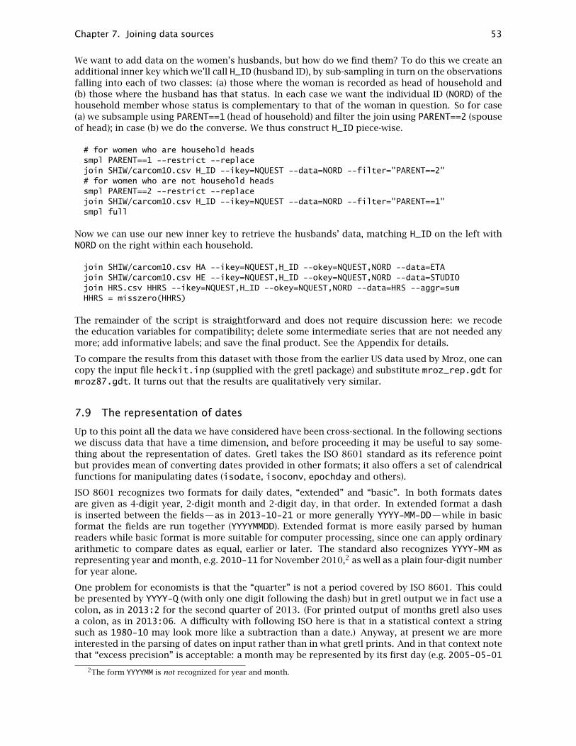
Chapter 7. Joining data sources 53
We want to add data on the women’s husbands, but how do we find them? To do this we create anadditional inner key which we’ll call H_ID (husband ID), by sub-sampling in turn on the observationsfalling into each of two classes: (a) those where the woman is recorded as head of household and(b) those where the husband has that status. In each case we want the individual ID (NORD) of thehousehold member whose status is complementary to that of the woman in question. So for case(a) we subsample using PARENT==1 (head of household) and filter the join using PARENT==2 (spouseof head); in case (b) we do the converse. We thus construct H_ID piece-wise.
# for women who are household headssmpl PARENT==1 --restrict --replacejoin SHIW/carcom10.csv H_ID --ikey=NQUEST --data=NORD --filter="PARENT==2"# for women who are not household headssmpl PARENT==2 --restrict --replacejoin SHIW/carcom10.csv H_ID --ikey=NQUEST --data=NORD --filter="PARENT==1"smpl full
Now we can use our new inner key to retrieve the husbands’ data, matching H_ID on the left withNORD on the right within each household.
join SHIW/carcom10.csv HA --ikey=NQUEST,H_ID --okey=NQUEST,NORD --data=ETAjoin SHIW/carcom10.csv HE --ikey=NQUEST,H_ID --okey=NQUEST,NORD --data=STUDIOjoin HRS.csv HHRS --ikey=NQUEST,H_ID --okey=NQUEST,NORD --data=HRS --aggr=sumHHRS = misszero(HHRS)
The remainder of the script is straightforward and does not require discussion here: we recodethe education variables for compatibility; delete some intermediate series that are not needed anymore; add informative labels; and save the final product. See the Appendix for details.
To compare the results from this dataset with those from the earlier US data used by Mroz, one cancopy the input file heckit.inp (supplied with the gretl package) and substitute mroz_rep.gdt formroz87.gdt. It turns out that the results are qualitatively very similar.
7.9 The representation of dates
Up to this point all the data we have considered have been cross-sectional. In the following sectionswe discuss data that have a time dimension, and before proceeding it may be useful to say some-thing about the representation of dates. Gretl takes the ISO 8601 standard as its reference pointbut provides mean of converting dates provided in other formats; it also offers a set of calendricalfunctions for manipulating dates (isodate, isoconv, epochday and others).
ISO 8601 recognizes two formats for daily dates, “extended” and “basic”. In both formats datesare given as 4-digit year, 2-digit month and 2-digit day, in that order. In extended format a dashis inserted between the fields—as in 2013-10-21 or more generally YYYY-MM-DD—while in basicformat the fields are run together (YYYYMMDD). Extended format is more easily parsed by humanreaders while basic format is more suitable for computer processing, since one can apply ordinaryarithmetic to compare dates as equal, earlier or later. The standard also recognizes YYYY-MM asrepresenting year and month, e.g. 2010-11 for November 2010,2 as well as a plain four-digit numberfor year alone.
One problem for economists is that the “quarter” is not a period covered by ISO 8601. This couldbe presented by YYYY-Q (with only one digit following the dash) but in gretl output we in fact use acolon, as in 2013:2 for the second quarter of 2013. (For printed output of months gretl also usesa colon, as in 2013:06. A difficulty with following ISO here is that in a statistical context a stringsuch as 1980-10 may look more like a subtraction than a date.) Anyway, at present we are moreinterested in the parsing of dates on input rather than in what gretl prints. And in that context notethat “excess precision” is acceptable: a month may be represented by its first day (e.g. 2005-05-01
2The form YYYYMM is not recognized for year and month.

Chapter 7. Joining data sources 54
for May, 2005), and a quarter may be represented by its first month and day (2005-07-01 for thethird quarter of 2005).
Some additional points regarding dates will be taken up as they become relevant in practical casesof joining data.
7.10 Time-series data
Suppose our left-hand dataset is recognized by gretl as time series with a supported frequency(annual, quarterly, monthly, weekly, daily or hourly). This will be the case if the original data wereread from a file that contained suitable time or date information, or if a time-series interpretationhas been imposed using either the setobs command or its GUI equivalent. Then—apart, perhaps,from some very special cases—joining additional data is bound to involve matching observationsby time-period.
In this case, contrary to the cross-sectional case, the inner dataset has a natural ordering whichgretl is aware of; hence, no “inner key” is required. All we need is a means of identifying the periodon the right and this is why, in a time-series context, we’ll refer to the outer key as the “time key”.Most likely, this information will appear in a single column in the outer data file, often but notalways the first column.
The join command provides a simple (but limited) default for extracting period information fromthe outer data file, plus an option that can be used if the default is not applicable, as follows.
• The default assumptions are: (1) the time key appears in the first column; (2) the headingof this column is either left blank or is one of obs, date, year, period, observation, orobservation_date (on a case-insensitive comparison); and (3) the time format conformsto ISO 8601 where applicable (“extended” daily date format YYYY-MM-DD, monthly formatYYYY-MM, or annual format YYYY).
• If dates do not appear in the first column of the outer file, or if the column heading or formatis not as just described, the --tkey option can be used to indicate which column should beused and/or what format should be assumed.
Setting the time-key column and/or format
The --tkey option requires a parameter holding the name of the column in which the time keyis located and/or a string specifying the format in which dates/times are written in the time-keycolumn. This parameter should be enclosed in double-quotes. If both elements are present theyshould be separated by a comma; if only a format is given it should be preceded by a comma. Someexamples:
--tkey="Period,%m/%d/%Y"--tkey="Period"--tkey="obsperiod"--tkey=",%Ym%m"
The first of these applies if Period is not the first column on the right, and dates are given in theUS format of month, day, year, separated by slashes. The second implies that although Period isnot the first column, the date format is ISO 8601. The third again implies that the date format isOK; here the name is required even if obsperiod is the first column since this heading is not onerecognized by gretl’s heuristic. The last example implies that dates are in the first column (withone of the recognized headings), but are given in the non-standard format year, “m”, month.
The date format string should be composed using the codes employed by the POSIX functionstrptime; Table 7.2 contains a list of the most relevant codes.3
3The %q code for quarter is not present in strptime; it is added for use with join since quarterly data are commonin macroeconomics.

Chapter 7. Joining data sources 55
Code Meaning
%% The % character.
%b The month name according to the current locale, either abbreviatedor in full.
%C The century number (0–99).
%d The day of month (1–31).
%D Equivalent to %m/%d/%y. (This is the American style date, very con-fusing to non-Americans, especially since %d/%m/%y is widely used inEurope. The ISO 8601 standard format is %Y-%m-%d.)
%H The hour (0–23).
%j The day number in the year (1–366).
%m The month number (1–12).
%n Arbitrary whitespace.
%q The quarter (1–4).
%w The weekday number (0–6) with Sunday = 0.
%y The year within century (0–99). When a century is not otherwise spec-ified, values in the range 69–99 refer to years in the twentieth century(1969–1999); values in the range 00–68 refer to years in the twenty-first century (2000–2068).
%Y The year, including century (for example, 1991).
Table 7.2: Date format codes
Example: daily stock prices
We show below the first few lines of a file named IBM.csv containing stock-price data for IBMcorporation.
Date,Open,High,Low,Close,Volume,Adj Close2013-08-02,195.50,195.50,193.22,195.16,3861000,195.162013-08-01,196.65,197.17,195.41,195.81,2856900,195.812013-07-31,194.49,196.91,194.49,195.04,3810000,195.04
Note that the data are in reverse time-series order—that won’t matter to join, the data can appearin any order. Also note that the first column is headed Date and holds daily dates as ISO 8601extended. That means we can pull the data into gretl very easily. In the following fragment wecreate a suitably dimensioned empty daily dataset then rely on the default behavior of join withtime-series data to import the closing stock price.
nulldata 500setobs 5 2012-01-01join IBM.csv Close
To make explicit what we’re doing, we could accomplish exactly the same using the --tkey option:
join IBM.csv Close --tkey="Date,%Y-%m-%d"
Example: OECD quarterly data
Table 7.3 shows an excerpt from a CSV file provided by the OECD statistical site (stat.oecd.org)in response to a request for GDP at constant prices for several countries.4
4Retrieved 2013-08-05. The OECD files in fact contain two leading columns with very long labels; these are irrelevantto the present example and can be omitted without altering the sample script.

Chapter 7. Joining data sources 56
Frequency,Period,Country,Value,Flags"Quarterly","Q1-1960","France",463876.148126845,E"Quarterly","Q1-1960","Germany",768802.119278467,E"Quarterly","Q1-1960","Italy",414629.791450547,E"Quarterly","Q1-1960","United Kingdom",578437.090291889,E"Quarterly","Q2-1960","France",465618.977328614,E"Quarterly","Q2-1960","Germany",782484.138122549,E"Quarterly","Q2-1960","Italy",420714.910290157,E"Quarterly","Q2-1960","United Kingdom",572853.474696578,E"Quarterly","Q3-1960","France",469104.41925852,E"Quarterly","Q3-1960","Germany",809532.161494483,E"Quarterly","Q3-1960","Italy",426893.675840156,E"Quarterly","Q3-1960","United Kingdom",581252.066618986,E"Quarterly","Q4-1960","France",474664.327992619,E"Quarterly","Q4-1960","Germany",817806.132384948,E"Quarterly","Q4-1960","Italy",427221.338414114,E...
Table 7.3: Example of CSV file as provided by the OECD statistical website
This is an instance of data in what we call atomic format, that is, a format in which each line of theouter file contains a single data-point and extracting data mainly requires filtering the appropriatelines. The outer time key is under the Period heading, and has the format Q<quarter>-<year>.Assuming that the file in Table 7.3 has the name oecd.csv, the following script reconstructs thetime series of Gross Domestic Product for several countries:
nulldata 220setobs 4 1960:1
join oecd.csv FRA --tkey="Period,Q%q-%Y" --data=Value --filter="Country==\"France\""join oecd.csv GER --tkey="Period,Q%q-%Y" --data=Value --filter="Country==\"Germany\""join oecd.csv ITA --tkey="Period,Q%q-%Y" --data=Value --filter="Country==\"Italy\""join oecd.csv UK --tkey="Period,Q%q-%Y" --data=Value --filter="Country==\"United Kingdom\""
Note the use of the format codes %q for the quarter and %Y for the 4-digit year. A touch of elegancecould have been added by storing the invariant options to join using the setopt command, as in
setopt join persist --tkey="Period,Q%q-%Y" --data=Valuejoin oecd.csv FRA --filter="Country==\"France\""join oecd.csv GER --filter="Country==\"Germany\""join oecd.csv ITA --filter="Country==\"Italy\""join oecd.csv UK --filter="Country==\"United Kingdom\""setopt join clear
If one were importing a large number of such series it might be worth rewriting the sequence ofjoins as a loop, as in
sprintf countries "France Germany Italy \"United Kingdom\""sprintf vnames "FRA GER ITA UK"setopt join persist --tkey="Period,Q%q-%Y" --data=Value
loop foreach i @countriesstring vname = strsplit(vnames, i)join oecd.csv @vname --filter="Country==\"$i\""
endloopsetopt join clear

Chapter 7. Joining data sources 57
7.11 Special handling of time columns
When dealing with straight time series data the tkey mechanism described above should sufficein almost all cases. In some contexts, however, time enters the picture in a more complex way;examples include panel data (see section 7.12) and so-called realtime data (see chapter 8). To handlesuch cases join provides the --tconvert option. This can be used to select certain columns inthe right-hand data file for special treatment: strings representing dates in these columns will beconverted to numerical values: 8-digit numbers on the pattern YYYYMMDD (ISO basic daily format).Once dates are in this form it is easy to use them in key-matching or filtering.
By default it is assumed that the strings in the selected columns are in ISO extended format,YYYY-MM-DD. If that is not the case you can supply a time-format string using the --tconv-fmtoption. The format string should be written using the codes shown in Table 7.2.
Here are some examples:
# select one column for treatment--tconvert=start_date
# select two columns for treatment--tconvert="start_date,end_date"
# specify US-style daily date format--tconv-fmt="%m/%d/%Y"
# specify quarterly date-strings (as in 2004q1)--tconv-fmt="%Yq%q"
Some points to note:
• If a specified column is not selected for a substantive role in the join operation (as data to beimported, as a key, or as an auxiliary variable for use in aggregation) the column in questionis not read and so no conversion is carried out.
• If a specified column contains numerical rather than string values, no conversion is carriedout.
• If a string value in a selected column fails parsing using the relevant time format (user-specified or default), the converted value is NA.
• On successful conversion, the output is always in daily-date form as stated above. If youspecify a monthly or quarterly time format, the converted date is the first day of the monthor quarter.
7.12 Panel data
In section 7.10 we gave an example of reading quarterly GDP data for several countries from anOECD file. In that context we imported each country’s data as a distinct time-series variable. Nowsuppose we want the GDP data in panel format instead (stacked time series). How can we do thiswith join?
As a reminder, here’s what the OECD data look like:
Frequency,Period,Country,Value,Flags"Quarterly","Q1-1960","France",463876.148126845,E"Quarterly","Q1-1960","Germany",768802.119278467,E"Quarterly","Q1-1960","Italy",414629.791450547,E"Quarterly","Q1-1960","United Kingdom",578437.090291889,E"Quarterly","Q2-1960","France",465618.977328614,E

Chapter 7. Joining data sources 58
and so on. If we have four countries and quarterly observations running from 1960:1 to 2013:2 (T= 214 quarters) we might set up our panel workspace like this:
scalar N = 4scalar T = 214scalar NT = N*Tnulldata NT --preservesetobs T 1.1 --stacked-time-series
The relevant outer keys are obvious: Country for the country and Period for the time period. Ourtask is now to construct matching keys in the inner dataset. This can be done via two panel-specificoptions to the setobs command. Let’s work on the time dimension first:
setobs 4 1960:1 --panel-timeseries quarter = $obsdate
This variant of setobs allows us to tell gretl that time in our panel is quarterly, starting in thefirst quarter of 1960. Having set that, the accessor $obsdate will give us a series of 8-digit datesrepresenting the first day of each quarter—19600101, 19600401, 19600701, and so on, repeatingfor each country. As we explained in section 7.11, we can use the --tconvert option on the outerseries Period to get exactly matching values (in this case using a format of Q%q-%Y for parsing thePeriod values).
Now for the country names:
string cstrssprintf cstrs "France Germany Italy \"United Kingdom\""setobs country cstrs --panel-groups
Here we write into the string cstrs the names of the countries, using escaped double-quotes tohandle the space in “United Kingdom”, then pass this string to setobs with the --panel-groupsoption, preceded by the identifier country. This asks gretl to construct a string-valued seriesnamed country, in which each name will repeat T times.
We’re now ready to join. Assuming the OECD file is named oecd.csv we do
join oecd.csv GDP --data=Value \--ikey=country,quarter --okey=Country,Period \--tconvert=Period --tconv-fmt="Q%q-%Y"
Other input formats
The OECD file discussed above is in the most convenient format for join, with one data-point perline. But sometimes we may want to make a panel from a data file structured like this:
# Real GDPPeriod,France,Germany,Italy,"United Kingdom""Q1-1960",463863,768757,414630,578437"Q2-1960",465605,782438,420715,572853"Q3-1960",469091,809484,426894,581252"Q4-1960",474651,817758,427221,584779"Q1-1961",482285,826031,442528,594684...
Call this file side_by_side.csv. Assuming the same initial set-up as above, we can panelize thedata by setting the sample to each country’s time series in turn and importing the relevant column.The only point to watch here is that the string “United Kingdom”, being a column heading, willbecome United_Kingdom on importing (see section 7.2) so we’ll need a slightly different set ofcountry strings.

Chapter 7. Joining data sources 59
sprintf cstrs "France Germany Italy United_Kingdom"setobs country cstrs --panel-groupsloop foreach i @cstrs --quietsmpl country=="$i" --restrict --replacejoin side_by_side.csv GDP --data=$i \--ikey=quarter --okey=Period \--tconvert=Period --tconv-fmt="Q%q-%Y"
endloopsmpl full
If our working dataset and the outer data file are dimensioned such that there are just as manytime-series observations on the right as there are time slots on the left—and the observationson the right are contiguous, in chronological order, and start on the same date as the workingdataset—we could dispense with the key apparatus and just use the first line of the join commandshown above. However, in general it is safer to use keys to ensure that the data end up in correctregistration.
7.13 Memo: join options
Basic syntax: join filename varname(s) [ options ]
flag effect
--data Give the name of the data column on the right, in case it differs fromvarname (7.2); single import only
--filter Specify a condition for filtering data rows (7.3)
--ikey Specify up to two keys for matching data rows (7.4)
--okey Specify outer key name(s) in case they differ the inner ones (7.4)
--aggr Select an aggregation method for 1 to n joins (7.5)
--tkey Specify right-hand time key (7.10)
--tconvert Select outer date columns for conversion to numeric form (7.11)
--tconv-fmt Specify a format for use with tconvert (7.11)
--no-header Treat the first row on the right as data (7.2)
--verbose Report on progress in reading the outer data

Chapter 7. Joining data sources 60
Appendix: the full Mroz data script
# start with everybody; get gender, age and a few other variables# directly while we’re at itopen SHIW/carcom10.csv --cols=1,2,3,4,9,10,29,41
# subsample on married women between the ages of 30 and 60smpl SEX==2 && ETA>=30 && ETA<=60 && STACIV==1 --restrict# for simplicity, restrict to heads of households and their spousessmpl PARENT<3 --restrict
# rename the age and education variables for compatibility; compute# the "city" dummy and finally save the reduced base datasetrename ETA WArename STUDIO WEseries CIT = (ACOM4C>2)store mroz_rep.gdt
# make a temp file holding annual hours worked per jobopen SHIW/allb1.csv --cols=1,2,8,11 --quietseries HRS = misszero(ORETOT) * 52 * misszero(MESILAV)/12store HRS.csv NQUEST NORD HRS
# reopen the base dataset and begin drawing assorted data inopen mroz_rep.gdt
# women’s annual hours (summed across jobs)join HRS.csv WHRS --ikey=NQUEST,NORD --data=HRS --aggr=sumWHRS = misszero(WHRS)
# labor force participationLFP = WHRS > 0
# work experience: ETALAV = age when started first jobjoin SHIW/lavoro.csv ETALAV --ikey=NQUEST,NORDseries AX = misszero(WA - ETALAV)
# women’s hourly wagesjoin SHIW/rper10.csv YL YM --ikey=NQUEST,NORD --aggr=sumseries WW = LFP ? (YL + YM)/WHRS : 0
# family income (Y = net disposable income)join SHIW/rfam10.csv FAMINC --ikey=NQUEST --data=Y
# get data on children using the "count" methodjoin SHIW/carcom10.csv KIDS --ikey=NQUEST --aggr=count --filter="ETA<=18"join SHIW/carcom10.csv KL6 --ikey=NQUEST --aggr=count --filter=ETA<6series K618 = KIDS - KL6
# data on husbands: we first construct an auxiliary inner key for# husbands, using the little trick of subsampling the inner dataset## for women who are household headssmpl PARENT==1 --restrict --replacejoin SHIW/carcom10.csv H_ID --ikey=NQUEST --data=NORD --filter="PARENT==2"# for women who are not household headssmpl PARENT==2 --restrict --replacejoin SHIW/carcom10.csv H_ID --ikey=NQUEST --data=NORD --filter="PARENT==1"smpl full
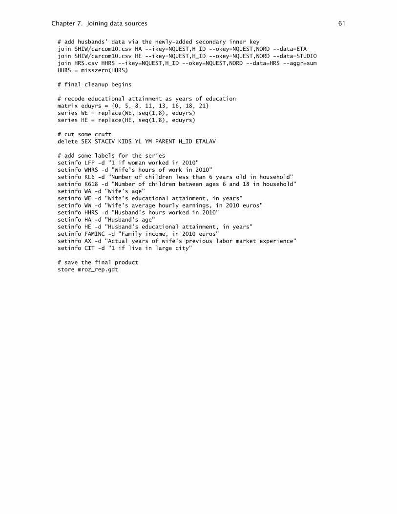
Chapter 7. Joining data sources 61
# add husbands’ data via the newly-added secondary inner keyjoin SHIW/carcom10.csv HA --ikey=NQUEST,H_ID --okey=NQUEST,NORD --data=ETAjoin SHIW/carcom10.csv HE --ikey=NQUEST,H_ID --okey=NQUEST,NORD --data=STUDIOjoin HRS.csv HHRS --ikey=NQUEST,H_ID --okey=NQUEST,NORD --data=HRS --aggr=sumHHRS = misszero(HHRS)
# final cleanup begins
# recode educational attainment as years of educationmatrix eduyrs = 0, 5, 8, 11, 13, 16, 18, 21series WE = replace(WE, seq(1,8), eduyrs)series HE = replace(HE, seq(1,8), eduyrs)
# cut some cruftdelete SEX STACIV KIDS YL YM PARENT H_ID ETALAV
# add some labels for the seriessetinfo LFP -d "1 if woman worked in 2010"setinfo WHRS -d "Wife’s hours of work in 2010"setinfo KL6 -d "Number of children less than 6 years old in household"setinfo K618 -d "Number of children between ages 6 and 18 in household"setinfo WA -d "Wife’s age"setinfo WE -d "Wife’s educational attainment, in years"setinfo WW -d "Wife’s average hourly earnings, in 2010 euros"setinfo HHRS -d "Husband’s hours worked in 2010"setinfo HA -d "Husband’s age"setinfo HE -d "Husband’s educational attainment, in years"setinfo FAMINC -d "Family income, in 2010 euros"setinfo AX -d "Actual years of wife’s previous labor market experience"setinfo CIT -d "1 if live in large city"
# save the final productstore mroz_rep.gdt

Chapter 8
Realtime data
8.1 Introduction
As of gretl version 1.9.13 the join command (see chapter 7) has been enhanced to deal with so-called realtime datasets in a straightforward manner. Such datasets contain information on whenthe observations in a time series were actually published by the relevant statistical agency and howthey have been revised over time. Probably the most popular sources of such data are the “Alfred”online database at the St. Louis Fed (http://alfred.stlouisfed.org/) and the OECD’s StatEx-tracts site, http://stats.oecd.org/. The examples in this chapter deal with files downloadedfrom these sources, but should be easy to adapt to files with a slightly different format.
As already stated, join requires a column-oriented plain text file, where the columns may be sepa-rated by commas, tabs, spaces or semicolons. Alfred and the OECD provide the option to downloadrealtime data in this format (tab-delimited files from Alfred, comma-delimited from the OECD). Ifyou have a realtime dataset in a spreadsheet file you must export it to a delimited text file beforeusing it with join.
Representing revision histories is more complex than just storing a standard time series, becausefor each observation period you have in general more than one published value over time, alongwith the information on when each of these values were valid or current. Sometimes this is repre-sented in spreadsheets with two time axes, one for the observation period and another one for thepublication date or “vintage”. The filled cells then form an upper triangle (or a “guillotine blade”shape, if the publication dates do not reach back far enough to complete the triangle). This formatcan be useful for giving a human reader an overview of realtime data, but it is not optimal forautomatic processing; for that purpose “atomic” format is best.
8.2 Atomic format for realtime data
What we are calling atomic format is exactly the format used by Alfred if you choose the option“Observations by Real-Time Period”, and by the OECD if you select all editions of a series fordownload as plain text (CSV).1 A file in this format contains one actual data-point per line, togetherwith associated metadata. This is illustrated in Table 8.1, where we show the first three lines froman Alfred file and an OECD file (slightly modified).2
Consider the first data line in the Alfred file: in the observation_date column we find 1960-01-01,indicating that the data-point on this line, namely 112.0, is an observation or measurement (in thiscase, of the US index of industrial production) that refers to the period starting on January 1st1960. The realtime_start_date value of 1960-02-16 tells us that this value was published onFebruary 16th 1960, and the realtime_end_date value says that this vintage remained currentthrough March 15th 1960. On the next day (as we can see from the following line) this data-pointwas revised slightly downward to 111.0.
Daily dates in Alfred files are given in ISO extended format, YYYY-MM-DD, but below we describehow to deal with differently formatted dates. Note that daily dates are appropriate for the last
1If you choose to download in Excel format from OECD you get a file in the triangular or guillotine format mentionedabove.
2In the Alfred file we have used commas rather than tabs as the column delimiter; in the OECD example we haveshortened the name in the Variable column.
62

Chapter 8. Realtime data 63
Alfred: monthly US industrial production
observation_date,INDPRO,realtime_start_date,realtime_end_date1960-01-01,112.0000,1960-02-16,1960-03-151960-01-01,111.0000,1960-03-16,1961-10-15
OECD: monthly UK industrial production
Country,Variable,Frequency,Time,Edition,Value,Flags"United Kingdom","INDPRO","Monthly","Jan-1990","February 1999",100,"United Kingdom","INDPRO","Monthly","Feb-1990","February 1999",99.3,
Table 8.1: Variant atomic formats for realtime data
two columns, which jointly record the interval over which a given data vintage was current. Dailydates might, however, be considered overly precise for the first column, since the data period maywell be the year, quarter or month (as it is in fact here). However, following Alfred’s practice it isacceptable to specify a daily date, indicating the first day of the period, even for non-daily data.3
Compare the first data line of the OECD example. There’s a greater amount of leading metadata,which is left implicit in the Alfred file. Here Time is the equivalent of Alfred’s observation_date,and Edition the equivalent of Alfred’s realtime_start_date. So we read that in February 1999a value of 100 was current for the UK index of industrial production for January 1990, and fromthe next line we see that in the same vintage month a value of 99.3 was current for industrialproduction in February 1990.
Besides the different names and ordering of the columns, there are a few more substantive differ-ences between Alfred and OECD files, most of which are irrelevant for join but some of which are(possibly) relevant.
The first (irrelevant) difference is the ordering of the lines. It appears (though we’re not sure howconsistent this is) that in Alfred files the lines are sorted by observation date first and then bypublication date—so that all revisions of a given observation are grouped together—while OECDfiles are sorted first by revision date (Edition) and then by observation date (Time). If we want thenext revision of UK industrial production for January 1990 in the OECD file we have to scan downseveral lines until we find
"United Kingdom","INDPRO","Monthly","Jan-1990","March 1999",100,
This difference is basically irrelevant because join can handle the case where the lines appear inrandom order, although some operations can be coded more conveniently if we’re able to assumechronological ordering (either on the Alfred or the OECD pattern, it doesn’t matter).
The second (also irrelevant) difference is that the OECD seems to include periodic “Edition” lineseven when there is no change from the previous value (as illustrated above, where the UK industrialproduction index for January 1990 is reported as 100 as of March 1999, the same value that we sawto be current in February 1999), while Alfred reports a new value only when it differs from whatwas previously current.
A third difference lies in the dating of the revisions or editions. As we have seen, Alfred givesa specific daily date while (in the UK industrial production file at any rate), the OECD just dateseach edition to a month. This is not necessarily relevant for join, but it does raise the question ofwhether the OECD might date revisions to a finer granularity in some of their files, in which caseone would have to be on the lookout for a different date format.
The final difference is that Alfred supplies an “end date” for each data vintage while the OECD
3Notice that this implies that in the Alfred example it is not clear without further information whether the observationperiod is the first quarter of 1960, the month January 1960, or the day January 1st 1960. However, we assume that thisinformation is always available in context.

Chapter 8. Realtime data 64
supplies only a starting date. But there is less to this difference than meets the eye: according tothe Alfred webmaster, “by design, a new vintage must start immediately following (the day after)the lapse of the old vintage”—so the end date conveys no independent information.4
8.3 More on time-related options
Before we get properly started it is worth saying a little more about the --tkey and --tconvertoptions to join (first introduced in section 7.11), as they apply in the case of realtime data.
When you’re working with regular time series data tkey is likely to be useful while tconvert isunlikely to be applicable (see section 7.10). On the other hand, when you’re working with panel datatkey is definitely not applicable but tconvert may well be helpful (section 7.12). When workingwith realtime data, however, depending on the task in hand both options may be useful. You willlikely need tkey; you may well wish to select at least one column for tconvert treatment; and infact you may want to name a given column in both contexts—that is, include the tkey variableamong the tconvert columns.
Why might this make sense? Well, think of the --tconvert option as a “preprocessing” directive:it asks gretl to convert date strings to numerical values (8-digit ISO basic dates) “at source”, as theyare read from the outer datafile. The --tkey option, on the other hand, singles out a column asthe one to use for matching rows with the inner dataset. So you would want to name a column inboth roles if (a) it should be used for matching periods and also (b) it is desirable to have the valuesfrom this column in numerical form, most likely for use in filtering.
As we have seen, you can supply specific formats in connection with both tkey and tconvert (inthe latter case via the companion option --tconv-fmt) to handle the case where the date strings onthe right are not ISO-friendly at source. This raises the question of how the format specificationswork if a given column is named under both options. Here are the rules that gretl applies:
1. If a format is given with the --tkey option it always applies to the tkey column alone; andfor that column it overrides any format given via the --tconv-fmt option.
2. If a format is given via tconv-fmt it is assumed to apply to all the tconvert columns, unlessthis assumption is overriden by rule 1.
8.4 Getting a certain data vintage
The most common application of realtime data is to “travel back in time” and retrieve the data thatwere current as of a certain date in the past. This would enable you to replicate a forecast or otherstatistical result that could have been produced at that date.
For example, suppose we are interested in a variable of monthly frequency named INDPRO, realtimedata on which is stored in an Alfred file named INDPRO.txt, and we want to check the status quoas of June 15th 2011.
If we don’t already have a suitable dataset into which to import the INDPRO data, our first steps willbe to create an appropriately dimensioned empty dataset using the nulldata command and thenspecify its time-series character via setobs, as in
nulldata 132setobs 12 2004:01
For convenience we can put the name of our realtime file into a string variable. On Windows thismight look like
4Email received from Travis May of the Federal Reserve Bank of St. Louis, 2013-10-17. This closes off the possibilitythat a given vintage could lapse or expire some time before the next vintage becomes available, hence giving rise to a“hole” in an Alfred realtime file.

Chapter 8. Realtime data 65
string fname = "C:/Users/yourname/Downloads/INDPRO.txt"
We can then import the data vintage 2011-06-15 using join, arbitrarily choosing the self-explanatoryidentifier ip_asof_20110615.
join @fname ip_asof_20110615 --tkey=observation_date --data=INDPRO \--tconvert="realtime_start_date" \--filter="realtime_start_date<=20110615" --aggr=max(realtime_start_date)
Here some detailed explanations of the various options are warranted:
• The --tkey option specifies the column which should be treated as holding the observationperiod identifiers to be matched against the periods in the current gretl dataset.5 The moregeneral form of this option is --tkey="colname,format" (note the double quotes here), soif the dates do not come in standard format, we can tell gretl how to parse them by usingthe appropriate conversion specifiers as shown in Table 7.2. For example, here we could havewritten --tkey="observation_date,%Y-%m-%d".
• Next, --data=INDPRO tells gretl that we want to retrieve the entries stored in the columnnamed INDPRO.
• As explained in section 7.11 the --tconvert option selects certain columns in the right-handdata file for conversion from date strings to 8-digit numbers on the pattern YYYYMMDD. We’llneed this for the next step, filtering, since the transformation to numerical values makesit possible to perform basic arithmetic on dates. Note that since date strings in Alfred filesconform to gretl’s default assumption it is not necessary to use the --tconv-fmt option here.
• The --filter option specification in combination with the subsequent --aggr aggregationtreatment is the central piece of our data retrieval; notice how we use the date constant20110615 in ISO basic form to do numerical comparisons, and how we perform the numericalmax operation on the converted column realtime_start_date. It would also have beenpossible to predefine a scalar variable, as in
vintage = 20110615
and then use vintage in the join command instead. Here we tell join that we only want toextract those publications that (1) already appeared before (and including) June 15th 2011,and (2) were not yet obsoleted by a newer release.6
As a result, your dataset will now contain a time series named ip_asof_20110615 with the valuesthat a researcher would have had available on June 15th 2011. Of course, all values for the observa-tions after June 2011 will be missing (and probably a few before that, too), because they only havebecome available later on.
8.5 Getting the n-th release for each observation period
For some purposes it may be useful to retrieve the n-th published value of each observation, wheren is a fixed positive integer, irrespective of when each of these n-th releases was published. Sup-pose we are interested in the third release, then the relevant join command becomes:
join @fname ip_3rdpub --tkey=observation_date --data=INDPRO --aggr="seq:3"
5Strictly speaking, using --tkey is unnecessary in this example because we could just have relied on the default,which is to use the first column in the source file for the periods. However, being explicit is often a good idea.
6By implementing the second condition through the max aggregation on the realtime_start_date column alone,without using the realtime_end_date column, we make use of the fact that Alfred files cannot have “holes” as explainedbefore.

Chapter 8. Realtime data 66
Since we do not need the realtime_start_date information for this retrieval, we have droppedthe --tconvert option here. Note that this formulation assumes that the source file is orderedchronologically, otherwise using the option --aggr="seq:3", which retrieves the third value fromeach sequence of matches, could have yielded a result different from the one intended. However,this assumption holds for Alfred files and is probably rather safe in general.
The values of the variable imported as ip_3rdpub in this way were published at different dates,so the variable is effectively a mix of different vintages. Depending on the type of variable, thismay also imply drastic jumps in the values; for example, index numbers are regularly re-basedto different base periods. This problem also carries over to inflation-adjusted economic variables,where the base period of the price index changes over time. Mixing vintages in general also meansmixing different scales in the output, with which you would have to deal appropriately.7
8.6 Getting the values at a fixed lag after the observation period
New data releases may take place on any day of the month, and as we have seen the specific dayof each release is recorded in realtime files from Alfred. However, if you are working with, say,monthly or quarterly data you may sometimes want to adjust the granularity of your realtime axisto a monthly or quarterly frequency. For example, in order to analyse the data revision process formonthly industrial production you might be interested in the extent of revisions between the dataavailable two and three months after each observation period.
This is a relatively complicated task and there is more than one way of accomplishing it. Either youhave to make several passes through the outer dataset or you need a sophisticated filter, writtenas a hansl function. Either way you will want to make use of some of gretl’s built-in calendricalfunctions.
We’ll assume that a suitably dimensioned workspace has been set up as described above. Giventhat, the key ingredients of the join are a filtering function which we’ll call rel_ok (for “release isOK”) and the join command which calls it. Here’s the function:
function series rel_ok (series obsdate, series reldate, int p)series y_obs, m_obs, y_rel, m_rel# get year and month from observation dateisoconv(obsdate, &y_obs, &m_obs)# get year and month from release dateisoconv(reldate, &y_rel, &m_rel)# find the delta in monthsseries dm = (12*y_rel + m_rel) - (12*y_obs + m_obs)# and implement the filterreturn dm <= p
end function
And here’s the command:
scalar lag = 3 # choose your fixed lag herejoin @fname ip_plus3 --data=INDPRO --tkey=observation_date \--tconvert="observation_date,realtime_start_date" \--filter="rel_ok(observation_date, realtime_start_date, lag)" \--aggr=max(realtime_start_date)
Note that we use --tconvert to convert both the observation date and the realtime start date (orrelease date) to 8-digit numerical values. Both of these series are passed to the filter, which uses the
7Some user-contributed functions may be available that address this issue, but it is beyond our scope here. Anothereven more complicated issue in the realtime context is that of “benchmark revisions” applied by statistical agencies,where the underlying definition or composition of a variable changes on some date, which goes beyond a mere rescaling.However, this type of structural change is not, in principle, a feature of realtime data alone, but applies to any time-seriesdata.

Chapter 8. Realtime data 67
built-in function isoconv to extract year and month. We can then calculate dm, the “delta months”since the observation date, for each release. The filter condition is that this delta should be nogreater than the specified lag, p.8
This filter condition may be satisfied by more than one release, but only the latest of those willactually be the vintage that was current at the end of the n-th month after the observation period,so we add the option --aggr=max(realtime_start_date). If instead you want to target therelease at the beginning of the n-th month you would have to use a slightly more complicated filterfunction.
An illustration
Figure 8.1 shows four time series for the monthly index of US industrial production from October2005 to June 2009: the value as of first publication plus the values current 3, 6 and 12 months outfrom the observation date.9 From visual inspection it would seem that over much of this periodthe Federal reserve was fairly consistently overestimating industrial production at first release andshortly thereafter, relative to the figure they arrived at with a lag of a year.
The script that produced this Figure is shown in full in Listing 8.1. Note that in this script we areusing a somewhat more efficient version of the rel_ok function shown above, where we pass therequired series arguments in “pointer” form to avoid having to copy them (see chapter 13).
94
96
98
100
102
104
106
108
110
112
114
116
2006 2007 2008 2009
First publicationPlus 3 monthsPlus 6 months
Plus 12 months
Figure 8.1: Successive revisions to US industrial production
8.7 Getting the revision history for an observation
For our final example we show how to retrieve the revision history for a given observation (againusing Alfred data on US industrial production). In this exercise we are switching the time axis: theobservation period is a fixed point and time is “vintage time”.
A suitable script is shown in Listing 8.2. We first select an observation to track (January 1970). Westart the clock in the following month, when a data-point for this period was first published, and let
8The filter is written on the assumption that the lag is expressed in months; on that understanding it could be usedwith annual or quarterly data as well as monthly. The idea could be generalized to cover weekly or daily data withoutmuch difficulty.
9Why not a longer series? Because if we try to extend it in either direction we immediately run into the index re-basingproblem mentioned in section 8.5, with big (staggered) leaps downward in all the series.

Chapter 8. Realtime data 68
Listing 8.1: Retrieving successive realtime lags of US industrial production
function series rel_ok (series *obsdate, series *reldate, int p)series y_obs, m_obs, y_rel, m_relisoconv(obsdate, &y_obs, &m_obs)isoconv(reldate, &y_rel, &m_rel)series dm = (12*y_rel + m_rel) - (12*y_obs + m_obs)return dm <= p
end function
nulldata 45setobs 12 2005:10
string fname = "INDPRO.txt"
# initial published valuesjoin @fname firstpub --data=INDPRO --tkey=observation_date \--tconvert=realtime_start_date --aggr=min(realtime_start_date)
# plus 3 monthsjoin @fname plus3 --data=INDPRO --tkey=observation_date \--tconvert="observation_date,realtime_start_date" \--filter="rel_ok(&observation_date, &realtime_start_date, 3)" \--aggr=max(realtime_start_date)
# plus 6 monthsjoin @fname plus6 --data=INDPRO --tkey=observation_date \--tconvert="observation_date,realtime_start_date" \--filter="rel_ok(&observation_date, &realtime_start_date, 6)" \--aggr=max(realtime_start_date)
# plus 12 monthsjoin @fname plus12 --data=INDPRO --tkey=observation_date \--tconvert="observation_date,realtime_start_date" \--filter="rel_ok(&observation_date, &realtime_start_date, 12)" \--aggr=max(realtime_start_date)
setinfo firstpub --graph-name="First publication"setinfo plus3 --graph-name="Plus 3 months"setinfo plus6 --graph-name="Plus 6 months"setinfo plus12 --graph-name="Plus 12 months"
gnuplot firstpub plus3 plus6 plus12 --time --with-lines \--output=realtime.pdf set key left bottom;

Chapter 8. Realtime data 69
it run to the end of the vintage history (in this file, March 2013). Our outer time key is the realtimestart date and we filter on observation date; we name the imported INDPRO values as ip_jan70.Since it sometimes happens that more than one revision occurs in a given month we need to selectan aggregation method: here we choose to take the last revision in the month.
Recall from section 8.2 that Alfred records a new revision only when the data-point in questionactually changes. This means that our imported series will contain missing values for all monthswhen no real revision took place. However, we can apply a simple autoregressive procedure to fillin the data: each missing value equals the prior non-missing value.
Figure 8.2 displays the revision history. Over this sample period the periodic re-basing of the indexovershadows amendments due to accrual of new information.
Listing 8.2: Retrieving a revision history
# choose the observation to track here (YYYYMMDD)scalar target = 19700101
nulldata 518 --preservesetobs 12 1970:02
join INDPRO.txt ip_jan70 --data=INDPRO --tkey=realtime_start_date \--tconvert=observation_date \--filter="observation_date==target" --aggr=seq:-1
ip_jan70 = ok(ip_jan70) ? ip_jan70 : ip_jan70(-1)
20
40
60
80
100
120
140
160
180
1970 1975 1980 1985 1990 1995 2000 2005 2010
ip_j
an7
0
Figure 8.2: Vintages of the index of US industrial production for January 1970

Chapter 9
Special functions in genr
9.1 Introduction
The genr command provides a flexible means of defining new variables. It is documented in theGretl Command Reference. This chapter offers a more expansive discussion of some of the specialfunctions available via genr and some of the finer points of the command.
9.2 Long-run variance
As is well known, the variance of the average of T random variables x1, x2, . . . , xT with equal vari-ance σ 2 equals σ 2/T if the data are uncorrelated. In this case, the sample variance of xt over thesample size provides a consistent estimator.
If, however, there is serial correlation among the xts, the variance of X = T−1∑Tt=1 xt must be
estimated differently. One of the most widely used statistics for this purpose is a nonparametrickernel estimator with the Bartlett kernel defined as
ω2(k) = T−1T−k∑t=k
k∑i=−k
wi(xt − X)(xt−i − X) , (9.1)
where the integer k is known as the window size and thewi terms are the so-called Bartlett weights,defined as wi = 1 − |i|
k+1 . It can be shown that, for k large enough, ω2(k)/T yields a consistentestimator of the variance of X.
Gretl implements this estimator by means of the function lrvar(), which takes two arguments:the series whose long-run variance must be estimated and the scalar k. If k is negative, the popularchoice T 1/3 is used.
9.3 Cumulative densities and p-values
The two functions cdf and pvalue provide complementary means of examining values from severalprobability distributions: the standard normal, Student’s t, χ2, F , gamma, and binomial. The syntaxof these functions is set out in the Gretl Command Reference; here we expand on some subtleties.
The cumulative density function or CDF for a random variable is the integral of the variable’sdensity from its lower limit (typically either −∞ or 0) to any specified value x. The p-value (atleast the one-tailed, right-hand p-value as returned by the pvalue function) is the complementaryprobability, the integral from x to the upper limit of the distribution, typically +∞.
In principle, therefore, there is no need for two distinct functions: given a CDF value p0 you couldeasily find the corresponding p-value as 1 − p0 (or vice versa). In practice, with finite-precisioncomputer arithmetic, the two functions are not redundant. This requires a little explanation. Ingretl, as in most statistical programs, floating point numbers are represented as “doubles” —double-precision values that typically have a storage size of eight bytes or 64 bits. Since there areonly so many bits available, only so many floating-point numbers can be represented: doubles donot model the real line. Typically doubles can represent numbers over the range (roughly) ±1.7977×10308, but only to about 15 digits of precision.
70

Chapter 9. Special functions in genr 71
Suppose you’re interested in the left tail of the χ2 distribution with 50 degrees of freedom: you’dlike to know the CDF value for x = 0.9. Take a look at the following interactive session:
? scalar p1 = cdf(X, 50, 0.9)Generated scalar p1 = 8.94977e-35? scalar p2 = pvalue(X, 50, 0.9)Generated scalar p2 = 1? scalar test = 1 - p2Generated scalar test = 0
The cdf function has produced an accurate value, but the pvalue function gives an answer of 1,from which it is not possible to retrieve the answer to the CDF question. This may seem surprisingat first, but consider: if the value of p1 above is correct, then the correct value for p2 is 1−8.94977×10⁻³⁵. But there’s no way that value can be represented as a double: that would require over 30digits of precision.
Of course this is an extreme example. If the x in question is not too far off into one or other tailof the distribution, the cdf and pvalue functions will in fact produce complementary answers, asshown below:
? scalar p1 = cdf(X, 50, 30)Generated scalar p1 = 0.0111648? scalar p2 = pvalue(X, 50, 30)Generated scalar p2 = 0.988835? scalar test = 1 - p2Generated scalar test = 0.0111648
But the moral is that if you want to examine extreme values you should be careful in selecting thefunction you need, in the knowledge that values very close to zero can be represented as doubleswhile values very close to 1 cannot.
9.4 Retrieving internal variables
The genr command provides a means of retrieving various values calculated by the program inthe course of estimating models or testing hypotheses. The variables that can be retrieved in thisway are listed in the Gretl Command Reference; here we say a bit more about the special variables$test and $pvalue.
These variables hold, respectively, the value of the last test statistic calculated using an explicittesting command and the p-value for that test statistic. If no such test has been performed at thetime when these variables are referenced, they will produce the missing value code. The “explicittesting commands” that work in this way are as follows: add (joint test for the significance of vari-ables added to a model); adf (Augmented Dickey–Fuller test, see below); arch (test for ARCH); chow(Chow test for a structural break); coeffsum (test for the sum of specified coefficients); cusum (theHarvey–Collier t-statistic); kpss (KPSS stationarity test, no p-value available); lmtest (see below);meantest (test for difference of means); omit (joint test for the significance of variables omittedfrom a model); reset (Ramsey’s RESET); restrict (general linear restriction); runs (runs test forrandomness); testuhat (test for normality of residual); and vartest (test for difference of vari-ances). In most cases both a $test and a $pvalue are stored; the exception is the KPSS test, forwhich a p-value is not currently available.
An important point to notice about this mechanism is that the internal variables $test and $pvalueare over-written each time one of the tests listed above is performed. If you want to reference thesevalues, you must do so at the correct point in the sequence of gretl commands.
A related point is that some of the test commands generate, by default, more than one test statisticand p-value; in these cases only the last values are stored. To get proper control over the retrievalof values via $test and $pvalue you should formulate the test command in such a way that theresult is unambiguous. This comment applies in particular to the adf and lmtest commands.

Chapter 9. Special functions in genr 72
• By default, the adf command generates three variants of the Dickey–Fuller test: one basedon a regression including a constant, one using a constant and linear trend, and one using aconstant and a quadratic trend. When you wish to reference $test or $pvalue in connectionwith this command, you can control the variant that is recorded by using one of the flags--nc, --c, --ct or --ctt with adf.
• By default, the lmtest command (which must follow an OLS regression) performs severaldiagnostic tests on the regression in question. To control what is recorded in $test and$pvalue you should limit the test using one of the flags --logs, --autocorr, --squares or--white.
As an aid in working with values retrieved using $test and $pvalue, the nature of the test to whichthese values relate is written into the descriptive label for the generated variable. You can read thelabel for the variable using the label command (with just one argument, the name of the variable),to check that you have retrieved the right value. The following interactive session illustrates thispoint.
? adf 4 x1 --cAugmented Dickey-Fuller tests, order 4, for x1sample size 59unit-root null hypothesis: a = 1test with constantmodel: (1 - L)y = b0 + (a-1)*y(-1) + ... + eestimated value of (a - 1): -0.216889test statistic: t = -1.83491asymptotic p-value 0.3638
P-values based on MacKinnon (JAE, 1996)? scalar pv = $pvalueGenerated scalar pv = 0.363844
9.5 The discrete Fourier transform
The discrete Fourier transform can be best thought of as a linear, invertible transform of a complexvector. Hence, if x is an n-dimensional vector whose k-th element is xk = ak+ ibk, then the outputof the discrete Fourier transform is a vector f = F(x) whose k-th element is
fk =n−1∑j=0
e−iω(j,k)xj
where ω(j, k) = 2πi jkn . Since the transformation is invertible, the vector x can be recovered fromf via the so-called inverse transform
xk =1n
n−1∑j=0
eiω(j,k)fj .
The Fourier transform is used in many diverse situations on account of this key property: theconvolution of two vectors can be performed efficiently by multiplying the elements of their Fouriertransforms and inverting the result. If
zk =n∑j=1
xjyk−j ,
thenF(z) = F(x)F(y).

Chapter 9. Special functions in genr 73
That is, F(z)k = F(x)kF(y)k.For computing the Fourier transform, gretl uses the external library fftw3: see Frigo and Johnson(2005). This guarantees extreme speed and accuracy. In fact, the CPU time needed to performthe transform is O(n logn) for any n. This is why the array of numerical techniques employed infftw3 is commonly known as the Fast Fourier Transform.
Gretl provides two matrix functions1 for performing the Fourier transform and its inverse: fft andffti. In fact, gretl’s implementation of the Fourier transform is somewhat more specialized: theinput to the fft function is understood to be real. Conversely, ffti takes a complex argument anddelivers a real result. For example:
matrix x1 = 1 ; 2 ; 3 # perform the transformmatrix f = fft(a)# perform the inverse transformmatrix x2 = ffti(f)
yields
x1 =
1
2
3
f =
6 0
−1.5 0.866
−1.5 −0.866
x2 =
1
2
3
where the first column of f holds the real part and the second holds the complex part. In general,if the input to fft has n columns, the output has 2n columns, where the real parts are stored inthe odd columns and the complex parts in the even ones. Should it be necessary to compute theFourier transform on several vectors with the same number of elements, it is numerically moreefficient to group them into a matrix rather than invoking fft for each vector separately.
As an example, consider the multiplication of two polynomials:
a(x) = 1+ 0.5xb(x) = 1+ 0.3x − 0.8x2
c(x) = a(x) · b(x) = 1+ 0.8x − 0.65x2 − 0.4x3
The coefficients of the polynomial c(x) are the convolution of the coefficients of a(x) and b(x);the following gretl code fragment illustrates how to compute the coefficients of c(x):
# define the two polynomialsa = 1, 0.5, 0, 0 ’b = 1, 0.3, -0.8, 0 ’# perform the transformsfa = fft(a)fb = fft(b)# complex-multiply the two transformsfc = cmult(fa, fb)# compute the coefficients of c via the inverse transformc = ffti(fc)
Maximum efficiency would have been achieved by grouping a and b into a matrix. The computa-tional advantage is so little in this case that the exercise is a bit silly, but the following alternativemay be preferable for a large number of rows/columns:
# define the two polynomialsa = 1 ; 0.5; 0 ; 0 b = 1 ; 0.3 ; -0.8 ; 0
1See chapter 16.

Chapter 9. Special functions in genr 74
# perform the transforms jointlyf = fft(a ~ b)# complex-multiply the two transformsfc = cmult(f[,1:2], f[,3:4])# compute the coefficients of c via the inverse transformc = ffti(fc)
Traditionally, the Fourier transform in econometrics has been mostly used in time-series analysis,the periodogram being the best known example. Listing 9.1 shows how to compute the periodogramof a time series via the fft function.
Listing 9.1: Periodogram via the Fourier transform
nulldata 50# generate an AR(1) processseries e = normal()series x = 0x = 0.9*x(-1) + e# compute the periodogramscale = 2*pi*$nobsX = x F = fft(X)S = sumr(F.^2)S = S[2:($nobs/2)+1]/scaleomega = seq(1,($nobs/2))’ .* (2*pi/$nobs)omega = omega ~ S# compare the built-in commandpergm xprint omega

Chapter 10
Gretl data types
10.1 Introduction
Gretl offers the following data types:
scalar holds a single numerical value
series holds n numerical values, where n is the number of observations in the currentdataset
matrix holds a rectangular array of numerical values, of any dimensions
list holds the ID numbers of a set of series
string holds an array of characters
bundle holds a variable number of objects of various types
array holds a variable number of objects of a given type
The “numerical values” mentioned above are all double-precision floating point numbers.
In this chapter we give a run-down of the basic characteristics of each of these types and alsoexplain their “life cycle” (creation, modification and destruction). The list and matrix types, whoseuses are relatively complex, are discussed at greater length in the following two chapters.
10.2 Series
We begin with the series type, which is the oldest and in a sense the most basic type in gretl. Whenyou open a data file in the gretl GUI, what you see in the main window are the ID numbers, names(and descriptions, if available) of the series read from the file. All the series existing at any point ina gretl session are of the same length, although some may have missing values. The variables thatcan be added via the items under the Add menu in the main window (logs, squares and so on) arealso series.
For a gretl session to contain any series, a common series length must be established. This isusually achieved by opening a data file, or importing a series from a database, in which case thelength is set by the first import. But one can also use the nulldata command, which takes as itsingle argument the desired length, a positive integer.
Each series has these basic attributes: an ID number, a name, and of course n numerical values.A series may also have a description (which is shown in the main window and is also accessiblevia the labels command), a “display name” for use in graphs, a record of the compaction methodused in reducing the variable’s frequency (for time-series data only) and a flag marking the variableas discrete. These attributes can be edited in the GUI by choosing Edit Attributes (either under theVariable menu or via right-click), or by means of the setinfo command.
In the context of most commands you are able to reference series by name or by ID number as youwish. The main exception is the definition or modification of variables via a formula; here you mustuse names since ID numbers would get confused with numerical constants.
Note that series ID numbers are always consecutive, and the ID number for a given series will changeif you delete a lower-numbered series. In some contexts, where gretl is liable to get confused bysuch changes, deletion of low-numbered series is disallowed.
75

Chapter 10. Gretl data types 76
Discrete series
It is possible to mark variables of the series type as discrete. The meaning and uses of this facilityare explained in chapter 11.
String-valued series
It is generally expected that series in gretl will be “properly numeric” (on a ratio or at least anordinal scale), or the sort of numerical indicator variables that are traditional in econometrics.However, there is some support for “string-valued” series—see chapter 15 for details.
10.3 Scalars
The scalar type is relatively simple: just a convenient named holder for a single numerical value.Scalars have none of the additional attributes pertaining to series, do not have ID numbers, andmust be referenced by name. A common use of scalar variables is to record information madeavailable by gretl commands for further processing, as in scalar s2 = $sigmaˆ2 to record thesquare of the standard error of the regression following an estimation command such as ols.
You can define and work with scalars in gretl without having any dataset in place.
In the gretl GUI, scalar variables can be inspected and their values edited via the “Icon view” (seethe View menu in the main window).
10.4 Matrices
Matrices in gretl work much as in other mathematical software (e.g. MATLAB, Octave). Like scalarsthey have no ID numbers and must be referenced by name, and they can be used without anydataset in place. Matrix indexing is 1-based: the top-left element of matrix A is A[1,1]. Matricesare discussed at length in chapter 16; advanced users of gretl will want to study this chapter indetail.
Matrices have two optional attribute beyond their numerical content: they may have column and/orrow names attached; these are displayed when the matrix is printed. See the colnames andrownames functions for details.
In the gretl GUI, matrices can be inspected, analysed and edited via the Icon view item under theView menu in the main window: each currently defined matrix is represented by an icon.
10.5 Lists
As with matrices, lists merit an explication of their own (see chapter 14). Briefly, named lists can(and should!) be used to make command scripts less verbose and repetitious, and more easilymodifiable. Since lists are in fact lists of series ID numbers they can be used only when a dataset isin place.
In the gretl GUI, named lists can be inspected and edited under the Data menu in the main window,via the item Define or edit list.
10.6 Strings
String variables may be used for labeling, or for constructing commands. They are discussed inchapter 14. They must be referenced by name; they can be defined in the absence of a dataset.
Such variables can be created and modified via the command-line in the gretl console or via script;there is no means of editing them via the gretl GUI.

Chapter 10. Gretl data types 77
10.7 Bundles
A bundle is a container or wrapper for various sorts of objects—specifically, scalars, series, ma-trices, strings, arrays and bundles. (Yes, a bundle can contain other bundles). A bundle takes theform of a hash table or associative array: each item placed in the bundle is associated with a keywhich can used to retrieve it subsequently. We begin by explaining the mechanics of bundles thenoffer some thoughts on what they are good for.
To use a bundle you first either “declare” it, as in
bundle foo
or define an empty bundle using the null keyword:
bundle foo = null
These two formulations are basically equivalent, in that they both create an empty bundle. Thedifference is that the second variant may be reused—if a bundle named foo already exists theeffect is to empty it—while the first may only be used once in a given gretl session; it is an error todeclare a variable that already exists.
To add an object to a bundle you assign to a compound left-hand value: the name of the bundlefollowed by the key. Two forms of syntax are acceptable in this context. The currently recom-mended syntax (for most uses) is bundlename.key ; that is, the name of the bundle followed by adot, then the key. Both the bundle name and the key must be valid gretl identifiers.1 For example,the statement
foo.matrix1 = m
adds an object called m (presumably a matrix) to bundle foo under the key matrix1. The originalsyntax (and the only form supported prior to version 1.9.12 of gretl) requires that the key be givenas a quoted string literal enclosed in square brackets, as in
foo["matrix1"] = m
This syntax is still acceptable, and it offers greater flexibility in that the key string does not haveto be a valid identifier (for example it can include spaces) though it still must adhere to the 31-character limit. In addition, when using the square bracket syntax it is possible to use a stringvariable to define or access the key in question. For example:
string s = "matrix 1"foo[s] = m # matrix is added under key "matrix 1"
To get an item out of a bundle, again use the name of the bundle followed by the key, as in
matrix bm = foo.matrix1# or using the alternative notationmatrix bm = foo["matrix1"]# or using a string variablematrix bm = foo[s]
Note that the key identifying an object within a given bundle is necessarily unique. If you reuse anexisting key in a new assignment, the effect is to replace the object which was previously storedunder the given key. It is not required that the type of the replacement object is the same as thatof the original.
1As a reminder: 31 characters maximum, starting with a letter and composed of just letters, numbers or underscore.

Chapter 10. Gretl data types 78
Also note that when you add an object to a bundle, what in fact happens is that the bundle acquiresa copy of the object. The external object retains its own identity and is unaffected if the bundledobject is replaced by another. Consider the following script fragment:
bundle foomatrix m = I(3)foo.mykey = mscalar x = 20foo.mykey = x
After the above commands are completed bundle foo does not contain a matrix under mykey, butthe original matrix m is still in good health.
To delete an object from a bundle use the delete command, with the bundle/key combination, asin
delete foo.mykey
This destroys the object associated with the key and removes the key from the hash table.
To determine whether a bundle contains an object associated with a given key, use the inbundle()function. This takes two arguments: the name of the bundle and the key string. The value returnedby this function is an integer which codes for the type of the object (0 for no match, 1 for scalar, 2for series, 3 for matrix, 4 for string, 5 for bundle and 6 for array). The function typestr() may beused to get the string corresponding to this code. For example:
scalar type = inbundle(foo, x)if type == 0print "x: no such object"
elseprintf "x is of type %s\n", typestr(type)
endif
Besides adding, accessing, replacing and deleting individual items, the other operations that aresupported for bundles are union, printing and deletion. As regards union, if bundles b1 and b2 aredefined you can say
bundle b3 = b1 + b2
to create a new bundle that is the union of the two others. The algorithm is: create a new bundlethat is a copy of b1, then add any items from b2 whose keys are not already present in the newbundle. (This means that bundle union is not commutative if the bundles have one or more keystrings in common.)
If b is a bundle and you say print b, you get a listing of the bundle’s keys along with the types ofthe corresponding objects, as in
? print bbundle b:x (scalar)mat (matrix)inside (bundle)
What are bundles good for?
Bundles are unlikely to be of interest in the context of standalone gretl scripts, but they can bevery useful in the context of complex function packages where a good deal of information has to

Chapter 10. Gretl data types 79
be passed around between the component functions (see Cottrell and Lucchetti, 2016). Instead ofusing a lengthy list of individual arguments, function A can bundle up the required data and passit to functions B and C , where relevant information can be extracted via a mnemonic key.
In this context bundles should be passed in “pointer” form (see chapter 13) as illustrated in the fol-lowing trivial example, where a bundle is created at one level then filled out by a separate function.
# modification of bundle (pointer) by user function
function void fill_out_bundle (bundle *b)b.mat = I(3)b.str = "foo"b.x = 32
end function
bundle my_bundlefill_out_bundle(&my_bundle)
The bundle type can also be used to advantage as the return value from a packaged function, incases where a package writer wants to give the user the option of accessing various results. Inthe gretl GUI, function packages that return a bundle are treated specially: the output window thatdisplays the printed results acquires a menu showing the bundled items (their names and types),from which the user can save items of interest. For example, a function package that estimates amodel might return a bundle containing a vector of parameter estimates, a residual series and acovariance matrix for the parameter estimates, among other possibilities.
As a refinement to support the use of bundles as a function return type, the setnote function canbe used to add a brief explanatory note to a bundled item—such notes will then be shown in theGUI menu. This function takes three arguments: the name of a bundle, a key string, and the note.For example
setnote(b, "vcv", "covariance matrix")
After this, the object under the key vcv in bundle b will be shown as “covariance matrix” in a GUImenu.
10.8 Arrays
The gretl array type was developed in summer 2014 and is first documented in gretl 1.10. Arraysare intended for scripting use only: they have no GUI representation and they’re unlikely everto acquire one.2 Since this type is a relative newcomer there are at present relatively few built-infunctions that take arrays as arguments or that return arrays; further development can be expected.
A gretl array is, as you might expect, a container which can hold zero or more objects of a certaintype, indexed by consecutive integers starting at 1. It is one-dimensional. This type is implementedby a quite “generic” back-end. The types of object that can be put into arrays are strings, matricesand bundles; a given array can hold only one of these types.
Of gretl’s “primary” types, then, neither scalars nor series are supported by the array mechanism.There would be little point in supporting arrays of scalars as such since the matrix type alreadyplays that role, and more flexibly. As for series, they have a special status as elements of a dataset(which is in a sense an “array of series” already) and in addition we have the list type which alreadyfunctions as a sort of array for subsets of the series in a dataset.
2However, it’s possible to save arrays “invisibly” in the context of a GUI session, by virtue of the fact that they can bepacked into bundles (see below), and bundles can be saved as part of a “session”.

Chapter 10. Gretl data types 80
Creating an array
An array can be brought into existence in any of four ways: bare declaration, assignment from null,or using one of the functions array() or defarray(). In each case one of the specific type-wordsstrings, matrices or bundles must be used. Here are some examples:
# make an empty array of stringsstrings S# make an empty array of matricesmatrices M = null# make an array with space for four bundlesbundles B = array(4)# make an array with three specified stringsstrings P = defarray("foo", "bar", "baz")
The “bare declaration” form and the “= null” form have the same effect of creating an empty array,but the second can be used in contexts where bare declaration is not allowed (and it can also beused to destroy the content of an existing array and reduce it to size zero). The array() functionexpects a positive integer argument and can be used to create an array of pre-given size; in thiscase the elements are initialized appropriately as empty strings, null matrices or empty bundles.The defarray() function takes a variable number of arguments (one or more), each of which maybe the name of a variable of the appropriate type or an expression which evaluates to an object ofthe appropriate type.
Setting and getting elements
There are two ways to set the value of an array element: you can set a particular element using thearray index, or you can append an element using the += operator:
# first casestrings S = array(3)S[2] = "string the second"# alternativematrices M = nullM += mnormal(T,k)
In the first method the index must (of course) be within bounds; that is, greater than zero andno greater than the current length of the array. When the second method is used it automaticallyextends the length of the array by 1.
To get hold of an element, the array index must be used:
# for S an array of stringsstring s = S[5]# for M an array of matricesprintf "\n%#12.5g\n", M[1]
Operations on whole arrays
At present only one operation is available for arrays as a whole, namely appending. You can do, forexample
# for S1 and S2 both arrays of stringsstrings BigS = S1 + S2# orS1 += S2
In each case the result is an array of strings whose length is the sum of the lengths of S1 andS2—and similarly for the other supported types.

Chapter 10. Gretl data types 81
Arrays as function arguments
One can write hansl functions that take as arguments any of the array types, and it is possible topass arrays as function arguments in “pointerized” form. In addition hansl functions may returnany of the array types. Here is a trivial example for strings:
function void printstrings (strings *S)loop i=1..nelem(S) -qprintf "element %d: ’%s’\n", i, S[i]
endloopend function
function strings mkstrs (int n)strings S = array(n)loop i=1..n -qS[i] = sprintf("member %d", i)
endloopreturn S
end function
strings Foo = mkstrs(5)print Fooprintstrings(&Foo)
A couple of points are worth noting here. First, the nelem() function works to give the number ofelements in any of the “container” types (lists, arrays, bundles, matrices). Second, if you do “printFoo” for Foo an array, you’ll see something like:
? print FooArray of strings, length 5
Arrays and bundles
As mentioned, the bundle type is supported by the array mechanism. In addition, arrays (of what-ever type) can be put into bundles:
matrices M = array(8)# set values of M[i] here...bundle bb.M = M
The mutual “packability” of bundles and arrays means that it’s possible to go quite far down therabbit-hole. . . users are advised not to get carried away.
10.9 The life cycle of gretl objects
Creation
The most basic way to create a new variable of any type is by declaration, where one states the typefollowed by the name of the variable to create, as in
scalar xseries ymatrix A
and so forth. In that case the object in question is given a default initialization, as follows: a newscalar has value NA (missing); a new series is filled with NAs; a new matrix is null (zero rows andcolumns); a new string is empty; a new list has no members, and a new bundle is empty.

Chapter 10. Gretl data types 82
Declaration can be supplemented by a definite initialization, as in
scalar x = piseries y = log(x)matrix A = zeros(10,4)
The traditional way of creating a new variable in gretl was via the genr command (which is stillsupported), as in
genr x = y/100
Here the type of x is left implicit and will be determined automatically depending on the context: ify is a scalar, a series or a matrix x will inherit y’s type (otherwise an error will be generated, sincedivision is applicable to these types only). Moreover, the type of a new variable can be left implicitwithout use of genr:3
x = y/100
In “modern” gretl scripting we recommend that you state the type of a new variable explicitly.This makes the intent clearer to a reader of the script and also guards against errors that mightotherwise be difficult to understand (i.e. a certain variable turns out to be of the wrong type forsome subsequent calculation, but you don’t notice at first because you didn’t say what type youneeded). An exception to this rule might reasonably be granted for clear and simple cases wherethere’s little possibility of confusion.
Modification
Typically, the values of variables of all types are modified by assignment, using the = operator withthe name of the variable on the left and a suitable value or formula on the right:
z = normal()x = 100 * log(y) - log(y(-1))M = qform(a, X)
By a “suitable” value we mean one that is conformable for the type in question. A gretl variableacquires its type when it is first created and this cannot be changed via assignment; for example, ifyou have a matrix A and later want a string A, you will have to delete the matrix first.
+ One point to watch out for in gretl scripting is type conflicts having to do with the names of series broughtin from a data file. For example, in setting up a command loop (see chapter 12) it is very common to callthe loop index i. Now a loop index is a scalar (typically incremented each time round the loop). If you opena data file that happens to contain a series named i you will get a type error (“Types not conformable foroperation”) when you try to use i as a loop index.
Although the type of an existing variable cannot be changed on the fly, gretl nonetheless tries to beas “understanding” as possible. For example if x is a series and you say
x = 100
gretl will give the series a constant value of 100 rather than complaining that you are trying toassign a scalar to a series. This issue is particularly relevant for the matrix type—see chapter 16for details.
Besides using the regular assignment operator you also have the option of using an “inflected”equals sign, as in the C programming language. This is shorthand for the case where the new valueof the variable is a function of the old value. For example,
3Apart from the bundle type: that must always be specified.

Chapter 10. Gretl data types 83
x += 100 # in longhand: x = x + 100x *= 100 # in longhand: x = x * 100
For scalar variables you can use a more condensed shorthand for simple increment or decrementby 1, namely trailing ++ or -- respectively:
x = 100x-- # x now equals 99x++ # x now equals 100
In the case of objects holding more than one value—series, matrices and bundles—you can mod-ify particular values within the object using an expression within square brackets to identify theelements to access. We have discussed this above for the bundle type and chapter 16 goes intodetails for matrices. As for series, there are two ways to specify particular values for modification:you can use a simple 1-based index, or if the dataset is a time series or panel (or if it has markerstrings that identify the observations) you can use an appropriate observation string. Such stringsare displayed by gretl when you print data with the --byobs flag. Examples:
x[13] = 100 # simple index: the 13th observationx[1995:4] = 100 # date: quarterly time seriesx[2003:08] = 100 # date: monthly time seriesx["AZ"] = 100 # the observation with marker string "AZ"x[3:15] = 100 # panel: the 15th observation for the 3rd unit
Note that with quarterly or monthly time series there is no ambiguity between a simple indexnumber and a date, since dates always contain a colon. With annual time-series data, however,such ambiguity exists and it is resolved by the rule that a number in brackets is always read as asimple index: x[1905] means the nineteen-hundred and fifth observation, not the observation forthe year 1905. You can specify a year by quotation, as in x["1905"].
Destruction
Objects of the types discussed above, with the important exception of named lists, are all destroyedusing the delete command: delete objectname.
Lists are an exception for this reason: in the context of gretl commands, a named list expands tothe ID numbers of the member series, so if you say
delete L
for L a list, the effect is to delete all the series in L; the list itself is not destroyed, but ends upempty. To delete the list itself (without deleting the member series) you must invert the commandand use the list keyword:
list L delete

Chapter 11
Discrete variables
When a variable can take only a finite, typically small, number of values, then it is said to be discrete.In gretl, variables of the series type (only) can be marked as discrete. (When we speak of “variables”below this should be understood as referring to series.) Some gretl commands act in a slightlydifferent way when applied to discrete variables; moreover, gretl provides a few commands thatonly apply to discrete variables. Specifically, the dummify and xtab commands (see below) areavailable only for discrete variables, while the freq (frequency distribution) command producesdifferent output for discrete variables.
11.1 Declaring variables as discrete
Gretl uses a simple heuristic to judge whether a given variable should be treated as discrete, butyou also have the option of explicitly marking a variable as discrete, in which case the heuristiccheck is bypassed.
The heuristic is as follows: First, are all the values of the variable “reasonably round”, where thisis taken to mean that they are all integer multiples of 0.25? If this criterion is met, we then askwhether the variable takes on a “fairly small” set of distinct values, where “fairly small” is definedas less than or equal to 8. If both conditions are satisfied, the variable is automatically considereddiscrete.
To mark a variable as discrete you have two options.
1. From the graphical interface, select “Variable, Edit Attributes” from the menu. A dialog boxwill appear and, if the variable seems suitable, you will see a tick box labeled “Treat thisvariable as discrete”. This dialog box can also be invoked via the context menu (right-click ona variable) or by pressing the F2 key.
2. From the command-line interface, via the discrete command. The command takes one ormore arguments, which can be either variables or list of variables. For example:
list xlist = x1 x2 x3discrete z1 xlist z2
This syntax makes it possible to declare as discrete many variables at once, which cannotpresently be done via the graphical interface. The switch --reverse reverses the declarationof a variable as discrete, or in other words marks it as continuous. For example:
discrete foo# now foo is discretediscrete foo --reverse# now foo is continuous
The command-line variant is more powerful, in that you can mark a variable as discrete even if itdoes not seem to be suitable for this treatment.
Note that marking a variable as discrete does not affect its content. It is the user’s responsibilityto make sure that marking a variable as discrete is a sensible thing to do. Note that if you want torecode a continuous variable into classes, you can use gretl’s arithmetical functionality, as in thefollowing example:
84
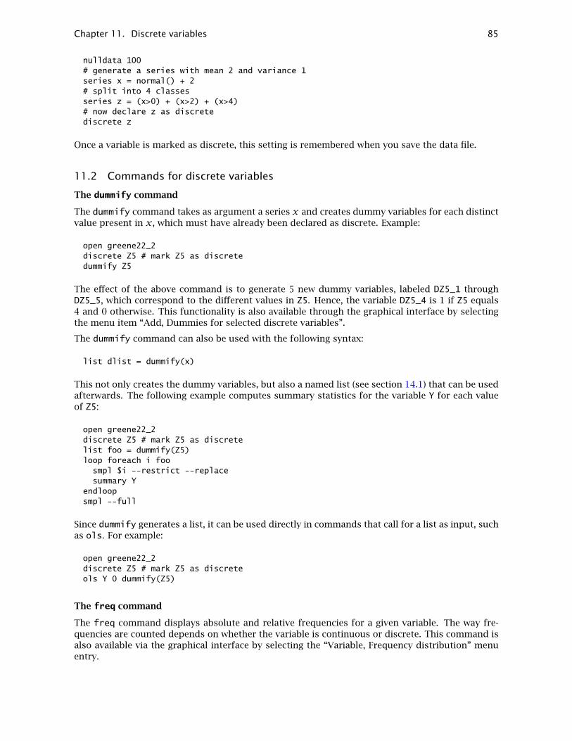
Chapter 11. Discrete variables 85
nulldata 100# generate a series with mean 2 and variance 1series x = normal() + 2# split into 4 classesseries z = (x>0) + (x>2) + (x>4)# now declare z as discretediscrete z
Once a variable is marked as discrete, this setting is remembered when you save the data file.
11.2 Commands for discrete variables
The dummify command
The dummify command takes as argument a series x and creates dummy variables for each distinctvalue present in x, which must have already been declared as discrete. Example:
open greene22_2discrete Z5 # mark Z5 as discretedummify Z5
The effect of the above command is to generate 5 new dummy variables, labeled DZ5_1 throughDZ5_5, which correspond to the different values in Z5. Hence, the variable DZ5_4 is 1 if Z5 equals4 and 0 otherwise. This functionality is also available through the graphical interface by selectingthe menu item “Add, Dummies for selected discrete variables”.
The dummify command can also be used with the following syntax:
list dlist = dummify(x)
This not only creates the dummy variables, but also a named list (see section 14.1) that can be usedafterwards. The following example computes summary statistics for the variable Y for each valueof Z5:
open greene22_2discrete Z5 # mark Z5 as discretelist foo = dummify(Z5)loop foreach i foosmpl $i --restrict --replacesummary Y
endloopsmpl --full
Since dummify generates a list, it can be used directly in commands that call for a list as input, suchas ols. For example:
open greene22_2discrete Z5 # mark Z5 as discreteols Y 0 dummify(Z5)
The freq command
The freq command displays absolute and relative frequencies for a given variable. The way fre-quencies are counted depends on whether the variable is continuous or discrete. This command isalso available via the graphical interface by selecting the “Variable, Frequency distribution” menuentry.

Chapter 11. Discrete variables 86
For discrete variables, frequencies are counted for each distinct value that the variable takes. Forcontinuous variables, values are grouped into “bins” and then the frequencies are counted for eachbin. The number of bins, by default, is computed as a function of the number of valid observationsin the currently selected sample via the rule shown in Table 11.1. However, when the command isinvoked through the menu item “Variable, Frequency Plot”, this default can be overridden by theuser.
Observations Bins
8 ≤ n < 16 5
16 ≤ n < 50 7
50 ≤ n ≤ 850 d√nen > 850 29
Table 11.1: Number of bins for various sample sizes
For example, the following code
open greene19_1freq TUCEdiscrete TUCE # mark TUCE as discretefreq TUCE
yields
Read datafile /usr/local/share/gretl/data/greene/greene19_1.gdtperiodicity: 1, maxobs: 32,observations range: 1-32
Listing 5 variables:0) const 1) GPA 2) TUCE 3) PSI 4) GRADE
? freq TUCE
Frequency distribution for TUCE, obs 1-32number of bins = 7, mean = 21.9375, sd = 3.90151
interval midpt frequency rel. cum.
< 13.417 12.000 1 3.12% 3.12% *13.417 - 16.250 14.833 1 3.12% 6.25% *16.250 - 19.083 17.667 6 18.75% 25.00% ******19.083 - 21.917 20.500 6 18.75% 43.75% ******21.917 - 24.750 23.333 9 28.12% 71.88% **********24.750 - 27.583 26.167 7 21.88% 93.75% *******
>= 27.583 29.000 2 6.25% 100.00% **
Test for null hypothesis of normal distribution:Chi-square(2) = 1.872 with p-value 0.39211? discrete TUCE # mark TUCE as discrete? freq TUCE
Frequency distribution for TUCE, obs 1-32
frequency rel. cum.
12 1 3.12% 3.12% *14 1 3.12% 6.25% *17 3 9.38% 15.62% ***

Chapter 11. Discrete variables 87
19 3 9.38% 25.00% ***20 2 6.25% 31.25% **21 4 12.50% 43.75% ****22 2 6.25% 50.00% **23 4 12.50% 62.50% ****24 3 9.38% 71.88% ***25 4 12.50% 84.38% ****26 2 6.25% 90.62% **27 1 3.12% 93.75% *28 1 3.12% 96.88% *29 1 3.12% 100.00% *
Test for null hypothesis of normal distribution:Chi-square(2) = 1.872 with p-value 0.39211
As can be seen from the sample output, a Doornik–Hansen test for normality is computed auto-matically. This test is suppressed for discrete variables where the number of distinct values is lessthan 10.
This command accepts two options: --quiet, to avoid generation of the histogram when invokedfrom the command line and --gamma, for replacing the normality test with Locke’s nonparametrictest, whose null hypothesis is that the data follow a Gamma distribution.
If the distinct values of a discrete variable need to be saved, the values() matrix construct can beused (see chapter 16).
The xtab command
The xtab command cab be invoked in either of the following ways. First,
xtab ylist ; xlist
where ylist and xlist are lists of discrete variables. This produces cross-tabulations (two-wayfrequencies) of each of the variables in ylist (by row) against each of the variables in xlist (bycolumn). Or second,
xtab xlist
In the second case a full set of cross-tabulations is generated; that is, each variable in xlist is tabu-lated against each other variable in the list. In the graphical interface, this command is representedby the “Cross Tabulation” item under the View menu, which is active if at least two variables areselected.
Here is an example of use:
open greene22_2discrete Z* # mark Z1-Z8 as discretextab Z1 Z4 ; Z5 Z6
which produces
Cross-tabulation of Z1 (rows) against Z5 (columns)
[ 1][ 2][ 3][ 4][ 5] TOT.
[ 0] 20 91 75 93 36 315[ 1] 28 73 54 97 34 286
TOTAL 48 164 129 190 70 601

Chapter 11. Discrete variables 88
Pearson chi-square test = 5.48233 (4 df, p-value = 0.241287)
Cross-tabulation of Z1 (rows) against Z6 (columns)
[ 9][ 12][ 14][ 16][ 17][ 18][ 20] TOT.
[ 0] 4 36 106 70 52 45 2 315[ 1] 3 8 48 45 37 67 78 286
TOTAL 7 44 154 115 89 112 80 601
Pearson chi-square test = 123.177 (6 df, p-value = 3.50375e-24)
Cross-tabulation of Z4 (rows) against Z5 (columns)
[ 1][ 2][ 3][ 4][ 5] TOT.
[ 0] 17 60 35 45 14 171[ 1] 31 104 94 145 56 430
TOTAL 48 164 129 190 70 601
Pearson chi-square test = 11.1615 (4 df, p-value = 0.0248074)
Cross-tabulation of Z4 (rows) against Z6 (columns)
[ 9][ 12][ 14][ 16][ 17][ 18][ 20] TOT.
[ 0] 1 8 39 47 30 32 14 171[ 1] 6 36 115 68 59 80 66 430
TOTAL 7 44 154 115 89 112 80 601
Pearson chi-square test = 18.3426 (6 df, p-value = 0.0054306)
Pearson’s χ2 test for independence is automatically displayed, provided that all cells have expectedfrequencies under independence greater than 10−7. However, a common rule of thumb states thatthis statistic is valid only if the expected frequency is 5 or greater for at least 80 percent of thecells. If this condition is not met a warning is printed.
Additionally, the --row or --column options can be given: in this case, the output displays row orcolumn percentages, respectively.
If you want to cut and paste the output of xtab to some other program, e.g. a spreadsheet, youmay want to use the --zeros option; this option causes cells with zero frequency to display thenumber 0 instead of being empty.

Chapter 12
Loop constructs
12.1 Introduction
The command loop opens a special mode in which gretl accepts a block of commands to be re-peated zero or more times. This feature may be useful for, among other things, Monte Carlosimulations, bootstrapping of test statistics and iterative estimation procedures. The general formof a loop is:
loop control-expression [ --progressive | --verbose | --quiet ]loop body
endloop
Five forms of control-expression are available, as explained in section 12.2.
Not all gretl commands are available within loops. The commands that are not presently acceptedin this context are shown in Table 12.1.
Table 12.1: Commands not usable in loops
function include nulldata run setmiss
By default, the genr command operates quietly in the context of a loop (without printing informa-tion on the variable generated). To force the printing of feedback from genr you may specify the--verbose option to loop. The --quiet option suppresses the usual printout of the number ofiterations performed, which may be desirable when loops are nested.
The --progressive option to loop modifies the behavior of the commands print and store,and certain estimation commands, in a manner that may be useful with Monte Carlo analyses (seeSection 12.3).
The following sections explain the various forms of the loop control expression and provide someexamples of use of loops.
+ If you are carrying out a substantial Monte Carlo analysis with many thousands of repetitions, memorycapacity and processing time may be an issue. To minimize the use of computer resources, run your scriptusing the command-line program, gretlcli, with output redirected to a file.
12.2 Loop control variants
Count loop
The simplest form of loop control is a direct specification of the number of times the loop shouldbe repeated. We refer to this as a “count loop”. The number of repetitions may be a numericalconstant, as in loop 1000, or may be read from a scalar variable, as in loop replics.
In the case where the loop count is given by a variable, say replics, in concept replics is aninteger; if the value is not integral, it is converted to an integer by truncation. Note that replics isevaluated only once, when the loop is initially compiled.
89

Chapter 12. Loop constructs 90
While loop
A second sort of control expression takes the form of the keyword while followed by a Booleanexpression. For example,
loop while essdiff > .00001
Execution of the commands within the loop will continue so long as (a) the specified conditionevaluates as true and (b) the number of iterations does not exceed the value of the internal variableloop_maxiter. By default this equals 100000, but you can specify a different value (or remove thelimit) via the set command (see the Gretl Command Reference).
Index loop
A third form of loop control uses an index variable, for example i.1 In this case you specify startingand ending values for the index, which is incremented by one each time round the loop. The syntaxlooks like this: loop i=1..20.
The index variable may be a pre-existing scalar; if this is not the case, the variable is createdautomatically and is destroyed on exit from the loop.
The index may be used within the loop body in either of two ways: you can access the integer valueof i or you can use its string representation, $i.
The starting and ending values for the index can be given in numerical form, by reference to pre-defined scalar variables, or as expressions that evaluate to scalars. In the latter two cases thevariables are evaluated once, at the start of the loop. In addition, with time series data you can givethe starting and ending values in the form of dates, as in loop i=1950:1..1999:4.
This form of loop control is intended to be quick and easy, and as such it is subject to certainlimitations. In particular, the index variable is always incremented by one at each iteration. If, forexample, you have
loop i=m..n
where m and n are scalar variables with values m > n at the time of execution, the index will not bedecremented; rather, the loop will simply be bypassed.
If you need more complex loop control, see the “for” form below.
The index loop is particularly useful in conjunction with the values() matrix function when someoperation must be carried out for each value of some discrete variable (see chapter 11). Considerthe following example:
open greene22_2discrete Z8v8 = values(Z8)loop i=1..rows(v8)scalar xi = v8[i]smpl Z8==xi --restrict --replaceprintf "mean(Y | Z8 = %g) = %8.5f, sd(Y | Z8 = %g) = %g\n", \xi, mean(Y), xi, sd(Y)
endloop
In this case, we evaluate the conditional mean and standard deviation of the variable Y for eachvalue of Z8.
1It is common programming practice to use simple, one-character names for such variables. However, you may useany name that is acceptable by gretl: up to 31 characters, starting with a letter, and containing nothing but letters,numerals and the underscore character.

Chapter 12. Loop constructs 91
Foreach loop
The fourth form of loop control also uses an index variable, in this case to index a specified listof strings. The loop is executed once for each string in the list. This can be useful for performingrepetitive operations on a list of variables. Here is an example of the syntax:
loop foreach i peach pear plumprint "$i"
endloop
This loop will execute three times, printing out “peach”, “pear” and “plum” on the respective itera-tions. The numerical value of the index starts at 1 and is incremented by 1 at each iteration.
If you wish to loop across a list of variables that are contiguous in the dataset, you can give thenames of the first and last variables in the list, separated by “..”, rather than having to type allthe names. For example, say we have 50 variables AK, AL, . . . , WY, containing income levels for thestates of the US. To run a regression of income on time for each of the states we could do:
genr timeloop foreach i AL..WY
ols $i const timeendloop
This loop variant can also be used for looping across the elements in a named list (see chapter 14).For example:
list ylist = y1 y2 y3loop foreach i ylist
ols $i const x1 x2endloop
Note that if you use this idiom inside a function (see chapter 13), looping across a list that has beensupplied to the function as an argument, it is necessary to use the syntax listname.$i to referencethe list-member variables. In the context of the example above, this would mean replacing the thirdline with
ols ylist.$i const x1 x2
For loop
The final form of loop control emulates the for statement in the C programming language. Thesytax is loop for, followed by three component expressions, separated by semicolons and sur-rounded by parentheses. The three components are as follows:
1. Initialization: This is evaluated only once, at the start of the loop. Common example: settinga scalar control variable to some starting value.
2. Continuation condition: this is evaluated at the top of each iteration (including the first). Ifthe expression evaluates as true (non-zero), iteration continues, otherwise it stops. Commonexample: an inequality expressing a bound on a control variable.
3. Modifier: an expression which modifies the value of some variable. This is evaluated priorto checking the continuation condition, on each iteration after the first. Common example: acontrol variable is incremented or decremented.
Here’s a simple example:

Chapter 12. Loop constructs 92
loop for (r=0.01; r<.991; r+=.01)
In this example the variable r will take on the values 0.01, 0.02, . . . , 0.99 across the 99 iterations.Note that due to the finite precision of floating point arithmetic on computers it may be necessaryto use a continuation condition such as the above, r<.991, rather than the more “natural” r<=.99.(Using double-precision numbers on an x86 processor, at the point where you would expect r toequal 0.99 it may in fact have value 0.990000000000001.)
Any or all of the three expressions governing a for loop may be omitted—the minimal form is(;;). If the continuation test is omitted it is implicitly true, so you have an infinite loop unless youarrange for some other way out, such as a break statement.
If the initialization expression in a for loop takes the common form of setting a scalar variable toa given value, the string representation of that scalar’s value is made available within the loop viathe accessor $varname.
12.3 Progressive mode
If the --progressive option is given for a command loop, special behavior is invoked for certaincommands, namely, print, store and simple estimation commands. By “simple” here we meancommands which (a) estimate a single equation (as opposed to a system of equations) and (b) doso by means of a single command statement (as opposed to a block of statements, as with nls andmle). The paradigm is ols; other possibilities include tsls, wls, logit and so on.
The special behavior is as follows.
Estimators: The results from each individual iteration of the estimator are not printed. Instead,after the loop is completed you get a printout of (a) the mean value of each estimated coefficientacross all the repetitions, (b) the standard deviation of those coefficient estimates, (c) the meanvalue of the estimated standard error for each coefficient, and (d) the standard deviation of theestimated standard errors. This makes sense only if there is some random input at each step.
print: When this command is used to print the value of a variable, you do not get a print each timeround the loop. Instead, when the loop is terminated you get a printout of the mean and standarddeviation of the variable, across the repetitions of the loop. This mode is intended for use withvariables that have a scalar value at each iteration, for example the error sum of squares from aregression. Data series cannot be printed in this way, and neither can matrices.
store: This command writes out the values of the specified scalars, from each time round theloop, to a specified file. Thus it keeps a complete record of their values across the iterations. Forexample, coefficient estimates could be saved in this way so as to permit subsequent examinationof their frequency distribution. Only one such store can be used in a given loop.
12.4 Loop examples
Monte Carlo example
A simple example of a Monte Carlo loop in “progressive” mode is shown in Listing 12.1.
This loop will print out summary statistics for the ‘a’ and ‘b’ estimates and R2 across the 100 rep-etitions. After running the loop, coeffs.gdt, which contains the individual coefficient estimatesfrom all the runs, can be opened in gretl to examine the frequency distribution of the estimates indetail.
The command nulldata is useful for Monte Carlo work. Instead of opening a “real” data set,nulldata 50 (for instance) opens a dummy data set, containing just a constant and an indexvariable, with a series length of 50. Constructed variables can then be added. See the set commandfor information on generating repeatable pseudo-random series.
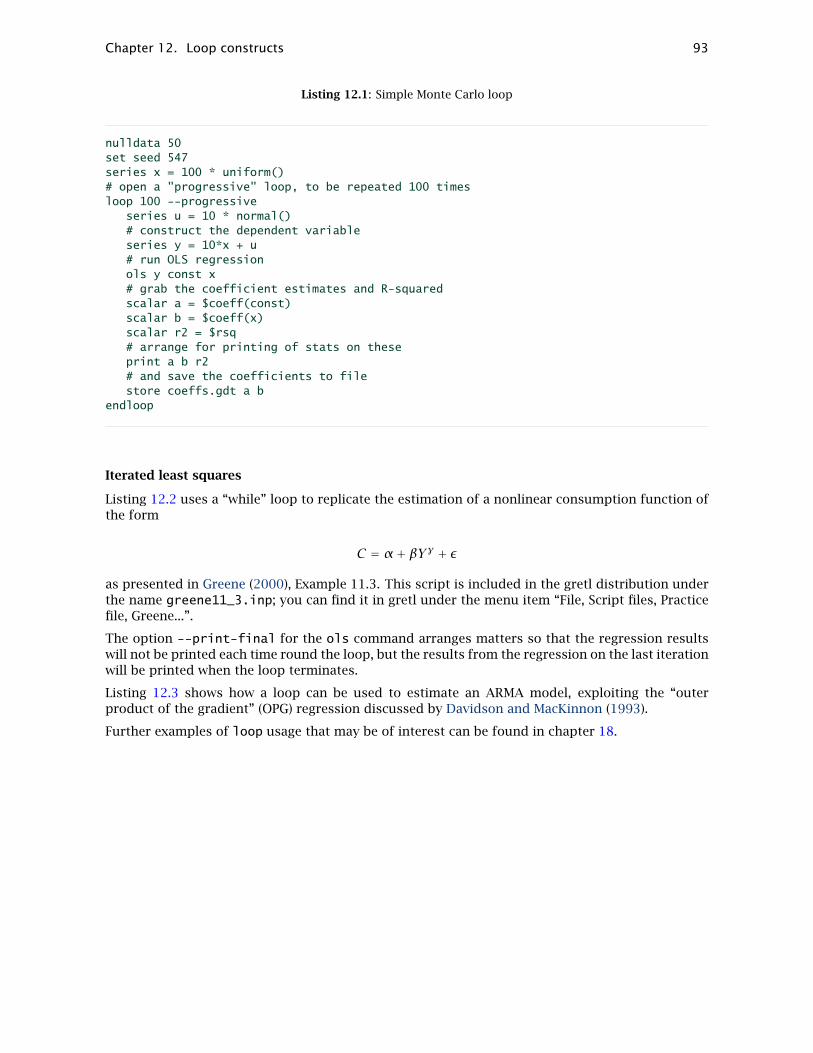
Chapter 12. Loop constructs 93
Listing 12.1: Simple Monte Carlo loop
nulldata 50set seed 547series x = 100 * uniform()# open a "progressive" loop, to be repeated 100 timesloop 100 --progressive
series u = 10 * normal()# construct the dependent variableseries y = 10*x + u# run OLS regressionols y const x# grab the coefficient estimates and R-squaredscalar a = $coeff(const)scalar b = $coeff(x)scalar r2 = $rsq# arrange for printing of stats on theseprint a b r2# and save the coefficients to filestore coeffs.gdt a b
endloop
Iterated least squares
Listing 12.2 uses a “while” loop to replicate the estimation of a nonlinear consumption function ofthe form
C = α+ βY γ + ε
as presented in Greene (2000), Example 11.3. This script is included in the gretl distribution underthe name greene11_3.inp; you can find it in gretl under the menu item “File, Script files, Practicefile, Greene...”.
The option --print-final for the ols command arranges matters so that the regression resultswill not be printed each time round the loop, but the results from the regression on the last iterationwill be printed when the loop terminates.
Listing 12.3 shows how a loop can be used to estimate an ARMA model, exploiting the “outerproduct of the gradient” (OPG) regression discussed by Davidson and MacKinnon (1993).
Further examples of loop usage that may be of interest can be found in chapter 18.

Chapter 12. Loop constructs 94
Listing 12.2: Nonlinear consumption function
open greene11_3.gdt# run initial OLSols C 0 Yscalar essbak = $essscalar essdiff = 1scalar beta = $coeff(Y)scalar gamma = 1
# iterate OLS till the error sum of squares convergesloop while essdiff > .00001
# form the linearized variablesseries C0 = C + gamma * beta * Y^gamma * log(Y)series x1 = Y^gammaseries x2 = beta * Y^gamma * log(Y)# run OLSols C0 0 x1 x2 --print-final --no-df-corr --vcvbeta = $coeff[2]gamma = $coeff[3]ess = $essessdiff = abs(ess - essbak)/essbakessbak = ess
endloop
# print parameter estimates using their "proper names"printf "alpha = %g\n", $coeff[1]printf "beta = %g\n", betaprintf "gamma = %g\n", gamma

Chapter 12. Loop constructs 95
Listing 12.3: ARMA 1, 1
# Estimation of an ARMA(1,1) model "manually", using a loop
open arma.gdt
scalar c = 0scalar a = 0.1scalar m = 0.1
series e = 0.0series de_c = eseries de_a = eseries de_m = e
scalar crit = 1
loop while crit > 1.0e-9 --quiet# one-step forecast errorse = y - c - a*y(-1) - m*e(-1)
# log-likelihoodscalar loglik = -0.5 * sum(e^2)print loglik
# partials of e with respect to c, a, and mde_c = -1 - m * de_c(-1)de_a = -y(-1) -m * de_a(-1)de_m = -e(-1) -m * de_m(-1)
# partials of l with respect to c, a and mseries sc_c = -de_c * eseries sc_a = -de_a * eseries sc_m = -de_m * e
# OPG regressionols const sc_c sc_a sc_m --print-final --no-df-corr --vcv
# Update the parametersc += $coeff[1]a += $coeff[2]m += $coeff[3]
# show progressprintf " constant = %.8g (gradient %#.6g)\n", c, $coeff[1]printf " ar1 coefficient = %.8g (gradient %#.6g)\n", a, $coeff[2]printf " ma1 coefficient = %.8g (gradient %#.6g)\n", m, $coeff[3]
crit = $T - $essprint crit
endloop
scalar se_c = $stderr[1]scalar se_a = $stderr[2]scalar se_m = $stderr[3]
printf "\n"printf "constant = %.8g (se = %#.6g, t = %.4f)\n", c, se_c, c/se_cprintf "ar1 coefficient = %.8g (se = %#.6g, t = %.4f)\n", a, se_a, a/se_aprintf "ma1 coefficient = %.8g (se = %#.6g, t = %.4f)\n", m, se_m, m/se_m

Chapter 13
User-defined functions
13.1 Defining a function
Gretl offers a mechanism for defining functions, which may be called via the command line, inthe context of a script, or (if packaged appropriately, see section 13.5) via the program’s graphicalinterface.
The syntax for defining a function looks like this:
function type funcname (parameters)function body
end function
The opening line of a function definition contains these elements, in strict order:
1. The keyword function.
2. type, which states the type of value returned by the function, if any. This must be one of void(if the function does not return anything), scalar, series, matrix, list, string, bundle orone of gretl’s array types, matrices, bundles, strings (see section 10.8).
3. funcname, the unique identifier for the function. Function names have a maximum length of31 characters; they must start with a letter and can contain only letters, numerals and theunderscore character. You will get an error if you try to define a function having the samename as an existing gretl command.
4. The function’s parameters, in the form of a comma-separated list enclosed in parentheses.This may be run into the function name, or separated by white space as shown. In case thefunction takes no arguments (unusual, but acceptable) this should be indicated by placing thekeyword void between the parameter-list parentheses.
Function parameters can be of any of the types shown below.1
Type Description
bool scalar variable acting as a Boolean switch
int scalar variable acting as an integer
scalar scalar variable
series data series
list named list of series
matrix matrix or vector
string string variable or string literal
bundle all-purpose container (see section 10.7)
matrices array of matrices (see section 10.8)
bundles array of bundles
strings array of strings
1An additional parameter type is available for GUI use, namely obs; this is equivalent to int except for the way it isrepresented in the graphical interface for calling a function.
96

Chapter 13. User-defined functions 97
Each element in the listing of parameters must include two terms: a type specifier, and the nameby which the parameter shall be known within the function. An example follows:
function scalar myfunc (series y, list xvars, bool verbose)
Each of the type-specifiers, with the exception of list and string, may be modified by prependingan asterisk to the associated parameter name, as in
function scalar myfunc (series *y, scalar *b)
The meaning of this modification is explained below (see section 13.4); it is related to the use ofpointer arguments in the C programming language.
Function parameters: optional refinements
Besides the required elements mentioned above, the specification of a function parameter mayinclude some additional fields, as follows:
• The const modifier.
• For scalar or int parameters: minimum, maximum and/or default values; or for bool pa-rameters, just a default value.
• For optional arguments in pointer form, and additionally for string or list arguments in stan-dard form (see section 13.4), the special default value null.
• For all parameters, a descriptive string.
• For int parameters with minimum and maximum values specified, a set of strings to associatewith the allowed numerical values (value labels).
The first two of these options may be useful in many contexts; the last two may be helpful if afunction is to be packaged for use in the gretl GUI (but probably not otherwise). We now expand oneach of the options.
• The const modifier: must be given as a prefix to the basic parameter specification, as in
const matrix M
This constitutes a promise that the corresponding argument will not be modified within thefunction; gretl will flag an error if the function attempts to modify the argument.
• Minimum, maximum and default values for scalar or int types: These values should di-rectly follow the name of the parameter, enclosed in square brackets and with the individualelements separated by colons. For example, suppose we have an integer parameter order forwhich we wish to specify a minimum of 1, a maximum of 12, and a default of 4. We can write
int order[1:12:4]
If you wish to omit any of the three specifiers, leave the corresponding field empty. Forexample [1::4] would specify a minimum of 1 and a default of 4 while leaving the maximumunlimited. However, as a special case, it is acceptable to give just one value, with no colons,in which case the value is interpreted as a default. So for example
int k[0]
designates a default value of 0 for the parameter k, with no minimum or maximum specified.If you wished to specify a minimum of zero with no maximum or default you would have towrite

Chapter 13. User-defined functions 98
int k[0::]
For a parameter of type bool (whose values are just zero or non-zero), you can specify adefault of 1 (true) or 0 (false), as in
bool verbose[0]
• Descriptive string: This will show up as an aid to the user if the function is packaged (seesection 13.5 below) and called via gretl’s graphical interface. The string should be enclosedin double quotes and separated from the preceding elements of the parameter specificationwith a space, as in
series y "dependent variable"
• Value labels: These may be used only with int parameters for which minimum and maximumvalues have been specified (so that there is a fixed number of admissible values) and thenumber of labels must match the number of values. They will show up in the graphicalinterface in the form of a drop-down list, making the function writer’s intent clearer when aninteger argument represents a categorical selection. A set of value labels must be enclosed inbraces, and the individual labels must be enclosed in double quotes and separated by commasor spaces. For example:
int case[1:3:1] "Fixed effects", "Between model", "Random effects"
If two or more of the trailing optional fields are given in a parameter specification, they must begiven in the order shown above: min/max/default, description, value labels. Note that there isno facility for “escaping” characters within descriptive strings or value labels; these may containspaces but they cannot contain the double-quote character.
Here is an example of a well-formed function specification using all the elements mentioned above:
function matrix myfunc (series y "dependent variable",list X "regressors",int p[0::1] "lag order",int c[1:2:1] "criterion" "AIC", "BIC",bool quiet[0])
One advantage of specifying default values for parameters, where applicable, is that in script orcommand-line mode users may omit trailing arguments that have defaults. For example, myfuncabove could be invoked with just two arguments, corresponding to y and X; implicitly p = 1, c = 1and quiet is false.
Functions taking no parameters
You may define a function that has no parameters (these are called “routines” in some programminglanguages). In this case, use the keyword void in place of the listing of parameters:
function matrix myfunc2 (void)
The function body
The function body is composed of gretl commands, or calls to user-defined functions (that is,function calls may be nested). A function may call itself (that is, functions may be recursive). Whilethe function body may contain function calls, it may not contain function definitions. That is, youcannot define a function inside another function. For further details, see section 13.4.

Chapter 13. User-defined functions 99
13.2 Calling a function
A user function is called by typing its name followed by zero or more arguments enclosed inparentheses. If there are two or more arguments they must be separated by commas.
There are automatic checks in place to ensure that the number of arguments given in a functioncall matches the number of parameters, and that the types of the given arguments match the typesspecified in the definition of the function. An error is flagged if either of these conditions is violated.One qualification: allowance is made for omitting arguments at the end of the list, provided thatdefault values are specified in the function definition. To be precise, the check is that the numberof arguments is at least equal to the number of required parameters, and is no greater than thetotal number of parameters.
In general, an argument to a function may be given either as the name of a pre-existing variable oras an expression which evaluates to a variable of the appropriate type.
The following trivial example illustrates a function call that correctly matches the correspondingfunction definition.
# function definitionfunction scalar ols_ess (series y, list xvars)ols y 0 xvars --quietprintf "ESS = %g\n", $essreturn $ess
end function
# main scriptopen data4-1list xlist = 2 3 4# function call (the return value is ignored here)ols_ess(price, xlist)
The function call gives two arguments: the first is a data series specified by name and the second isa named list of regressors. Note that while the function offers the Error Sum of Squares as a returnvalue, it is ignored by the caller in this instance. (As a side note here, if you want a function tocalculate some value having to do with a regression, but are not interested in the full results of theregression, you may wish to use the --quiet flag with the estimation command as shown above.)
A second example shows how to write a function call that assigns a return value to a variable in thecaller:
# function definitionfunction series get_uhat (series y, list xvars)ols y 0 xvars --quietreturn $uhat
end function
# main scriptopen data4-1list xlist = 2 3 4# function callseries resid = get_uhat(price, xlist)
13.3 Deleting a function
If you have defined a function and subsequently wish to clear it out of memory, you can do so usingthe keywords delete or clear, as in
function myfunc deletefunction get_uhat clear

Chapter 13. User-defined functions 100
Note, however, that if myfunc is already a defined function, providing a new definition automaticallyoverwrites the previous one, so it should rarely be necessary to delete functions explicitly.
13.4 Function programming details
Variables versus pointers
Most arguments to functions can be passed in two ways: “as they are”, or via pointers (the exceptionis the list type, which cannot be passed as a pointer). First consider the following rather artificialexample:
function series triple1 (series x)return 3*x
end function
function void triple2 (series *x)x *= 3
end function
nulldata 10series y = normal()series y3 = triple1(y)print y3triple2(&y)print y
These two functions produce essentially the same result—the two print statements in the callerwill show the same values—but in quite different ways. The first explicitly returns a modifiedversion of its input (which must be a plain series): after the call to triple1, y is unaltered; itwould have been altered only if the return value were assigned back to y rather than y3. Thesecond function modifies its input (given as a pointer to a series) in place without actually returninganything.
It’s worth noting that triple2 as it stands would not be considered idiomatic as a gretl function(although it’s formally OK). The point here is just to illustrate the distinction between passing anargument in the default way and in pointer form.
Why make this distinction? There are two main reasons for doing so: modularity and performance.
By modularity we mean the insulation of a function from the rest of the script which calls it. One ofthe many benefits of this approach is that your functions are easily reusable in other contexts. Toachieve modularity, variables created within a function are local to that function, and are destroyedwhen the function exits, unless they are made available as return values and these values are “pickedup” or assigned by the caller. In addition, functions do not have access to variables in “outer scope”(that is, variables that exist in the script from which the function is called) except insofar as theseare explicitly passed to the function as arguments.
By default, when a variable is passed to a function as an argument, what the function actually “gets”is a copy of the outer variable, which means that the value of the outer variable is not modified byanything that goes on inside the function. This means that you can pass arguments to a functionwithout worrying about possible side effects; at the same time the function writer can use argumentvariables as workspace without fear of disruptive effects at the level of the caller.
The use of pointers, however, allows a function and its caller to cooperate such that an outervariable can be modified by the function. In effect, this allows a function to “return” more than onevalue (although only one variable can be returned directly—see below). To indicate that a particularobject is to be passed as a pointer, the parameter in question is marked with a prefix of * in thefunction definition, and the corresponding argument is marked with the complementary prefix & inthe caller. For example,

Chapter 13. User-defined functions 101
function series get_uhat_and_ess(series y, list xvars, scalar *ess)ols y 0 xvars --quietess = $essseries uh = $uhatreturn uh
end function
open data4-1list xlist = 2 3 4scalar SSRseries resid = get_uhat_and_ess(price, xlist, &SSR)
In the above, we may say that the function is given the address of the scalar variable SSR, and itassigns a value to that variable (under the local name ess). (For anyone used to programming in C:note that it is not necessary, or even possible, to “dereference” the variable in question within thefunction using the * operator. Unadorned use of the name of the variable is sufficient to access thevariable in outer scope.)
An “address” parameter of this sort can be used as a means of offering optional information to thecaller. (That is, the corresponding argument is not strictly needed, but will be used if present). Inthat case the parameter should be given a default value of null and the the function should test tosee if the caller supplied a corresponding argument or not, using the built-in function exists().For example, here is the simple function shown above, modified to make the filling out of the essvalue optional.
function series get_uhat_and_ess(series y, list xvars, scalar *ess[null])ols y 0 xvars --quietif exists(ess)
ess = $essendifreturn $uhat
end function
If the caller does not care to get the ess value, it can use null in place of a real argument:
series resid = get_uhat_and_ess(price, xlist, null)
Alternatively, trailing function arguments that have default values may be omitted, so the followingwould also be a valid call:
series resid = get_uhat_and_ess(price, xlist)
One limitation on the use of pointer-type arguments should be noted: you cannot supply a givenvariable as a pointer argument more than once in any given function call. For example, suppose wehave a function that takes two matrix-pointer arguments,
function scalar pointfunc (matrix *a, matrix *b)
And suppose we have two matrices, x and y, at the caller level. The call
pointfunc(&x, &y)
is OK, but the call
pointfunc(&x, &x) # will not work
will generate an error. That’s because the situation inside the function would become too confusing,with what is really the same object existing under two names.

Chapter 13. User-defined functions 102
Const parameters
Pointer-type arguments may also be useful for optimizing performance. Even if a variable is notmodified inside the function, it may be a good idea to pass it as a pointer if it occupies a lot ofmemory. Otherwise, the time gretl spends transcribing the value of the variable to the local copymay be non-negligible compared to the time the function spends doing the job it was written for.
Listing 13.1 takes this to the extreme. We define two functions which return the number of rowsof a matrix (a pretty fast operation). The first gets a matrix as argument while the second gets apointer to a matrix. The functions are evaluated 500 times on a matrix with 2000 rows and 2000columns; on a typical system floating-point numbers take 8 bytes of memory, so the total size ofthe matrix is roughly 32 megabytes.
Running the code in example 13.1 will produce output similar to the following (the actual numbersof course depend on the machine you’re using):
Elapsed time:without pointers (copy) = 2.47197 seconds,with pointers (no copy) = 0.00378627 seconds
Listing 13.1: Performance comparison: values versus pointer
function scalar rowcount1 (matrix X)return rows(X)
end function
function scalar rowcount2 (const matrix *X)return rows(X)
end function
set verbose offX = zeros(2000,2000)scalar r
set stopwatchloop 500 -qr = rowcount1(X)
endloope1 = $stopwatch
set stopwatchloop 500 -qr = rowcount2(&X)
endloope2 = $stopwatch
printf "Elapsed time:\n\without pointers (copy) = %g seconds,\n \with pointers (no copy) = %g seconds\n", e1, e2
If a pointer argument is used for this sort of purpose—and the object to which the pointer pointsis not modified (is treated as read-only) by the function—one can signal this to the user by addingthe const qualifier, as shown for function rowcount2 in Listing 13.1. When a pointer argument isqualified in this way, any attempt to modify the object within the function will generate an error.
However, combining the const flag with the pointer mechanism is technically redundant for the

Chapter 13. User-defined functions 103
following reason: if you mark a matrix argument as const then gretl will in fact pass it in pointermode internally (since it can’t be modified within the function there’s no downside to simply mak-ing it available to the function rather than copying it). So in the example above we could revise thesignature of the second function as
function scalar rowcount2a (const matrix X)
and call it with r = rowcount2a(X), for the same speed-up relative to rowcount1.
From the caller’s point of view the second option—using the const modifier without pointernotation—is preferable, as it allows the caller to pass an object created “on the fly”. Supposethe caller has two matrices, A and B, in scope, and wishes to pass their vertical concatenation as anargument. The following call would work fine:
r = rowcount2a(A|B)
To use rowcount2, on the other hand, the caller would have to create a named variable first (sinceyou cannot give the “address” of a anonymous object such as A|B):
matrix AB = A|Br = rowcount2(&AB)
This requires an extra line of code, and leaves AB occupying memory after the call.
We have illusrated using a matrix parameter, but the const modifier may be used with the sameeffect—namely, the argument is passed directly, without being copied, but is protected againstmodification within the function—for all the types that support the pointer apparatus.
List arguments
The use of a named list as an argument to a function gives a means of supplying a function witha set of variables whose number is unknown when the function is written—for example, sets ofregressors or instruments. Within the function, the list can be passed on to commands such asols.
A list argument can also be “unpacked” using a foreach loop construct, but this requires somecare. For example, suppose you have a list X and want to calculate the standard deviation of eachvariable in the list. You can do:
loop foreach i Xscalar sd_$i = sd(X.$i)
endloop
Please note: a special piece of syntax is needed in this context. If we wanted to perform the abovetask on a list in a regular script (not inside a function), we could do
loop foreach i Xscalar sd_$i = sd($i)
endloop
where $i gets the name of the variable at position i in the list, and sd($i) gets its standarddeviation. But inside a function, working on a list supplied as an argument, if we want to referencean individual variable in the list we must use the syntax listname.varname. Hence in the exampleabove we write sd(X.$i).
This is necessary to avoid possible collisions between the name-space of the function and the name-space of the caller script. For example, suppose we have a function that takes a list argument, andthat defines a local variable called y. Now suppose that this function is passed a list containing

Chapter 13. User-defined functions 104
a variable named y. If the two name-spaces were not separated either we’d get an error, or theexternal variable y would be silently over-written by the local one. It is important, therefore, thatlist-argument variables should not be “visible” by name within functions. To “get hold of” suchvariables you need to use the form of identification just mentioned: the name of the list, followedby a dot, followed by the name of the variable.
Constancy of list arguments When a named list of variables is passed to a function, the functionis actually provided with a copy of the list. The function may modify this copy (for instance, addingor removing members), but the original list at the level of the caller is not modified.
Optional list arguments If a list argument to a function is optional, this should be indicated byappending a default value of null, as in
function scalar myfunc (scalar y, list X[null])
In that case, if the caller gives null as the list argument (or simply omits the last argument) thenamed list X inside the function will be empty. This possibility can be detected using the nelem()function, which returns 0 for an empty list.
String arguments
String arguments can be used, for example, to provide flexibility in the naming of variables createdwithin a function. In the following example the function mavg returns a list containing two movingaverages constructed from an input series, with the names of the newly created variables governedby the string argument.
function list mavg (series y, string vname)list retlist = nullstring newname = sprintf("%s_2", vname)retlist += genseries(newname, (y+y(-1)) / 2)newname = sprintf("%s_4", vname)retlist += genseries(newname, (y+y(-1)+y(-2)+y(-3)) / 4)return retlist
end function
open data9-9list malist = mavg(nocars, "nocars")print malist --byobs
The last line of the script will print two variables named nocars_2 and nocars_4. For details onthe handling of named strings, see chapter 14.
If a string argument is considered optional, it may be given a null default value, as in
function scalar foo (series y, string vname[null])
Retrieving the names of arguments
The variables given as arguments to a function are known inside the function by the names of thecorresponding parameters. For example, within the function whose signature is
function void somefun (series y)
we have the series known as y. It may be useful, however, to be able to determine the names ofthe variables provided as arguments. This can be done using the function argname, which takesthe name of a function parameter as its single argument and returns a string. Here is a simpleillustration:

Chapter 13. User-defined functions 105
function void namefun (series y)printf "the series given as ’y’ was named %s\n", argname(y)
end function
open data9-7namefun(QNC)
This produces the output
the series given as ’y’ was named QNC
Please note that this will not always work: the arguments given to functions may be anonymousvariables, created on the fly, as in somefun(log(QNC)) or somefun(CPI/100). In that case theargname function returns an empty string. Function writers who wish to make use of this facilityshould check the return from argname using the strlen() function: if this returns 0, no name wasfound.
Return values
Functions can return nothing (just printing a result, perhaps), or they can return a single variable.The return value, if any, is specified via a statement within the function body beginning with thekeyword return, followed by either the name of a variable (which must be of the type announcedon the first line of the function definition) or an expression which produces a value of the correcttype.
Having a function return a list or bundle is a way of permitting the “return” of more than onevariable. For example, you can define several series inside a function and package them as a list;in this case they are not destroyed when the function exits. Here is a simple example, which alsoillustrates the possibility of setting the descriptive labels for variables generated in a function.
function list make_cubes (list xlist)list cubes = nullloop foreach i xlist --quiet
series $i3 = (xlist.$i)^3setinfo $i3 -d "cube of $i"list cubes += $i3
endloopreturn cubes
end function
open data4-1list xlist = price sqftlist cubelist = make_cubes(xlist)print xlist cubelist --byobslabels
A return statement causes the function to return (exit) at the point where it appears within thebody of the function. A function may also exit when (a) the end of the function code is reached (inthe case of a function with no return value), (b) a gretl error occurs, or (c) a funcerr statement isreached.
The funcerr keyword—which may be followed by a string enclosed in double quotes, or the nameof a string variable, or nothing—causes a function to exit with an error flagged. If a string isprovided (either literally or via a variable), this is printed on exit, otherwise a generic error messageis printed. This mechanism enables the author of a function to pre-empt an ordinary executionerror and/or offer a more specific and helpful error message. For example,
if nelem(xlist) == 0funcerr "xlist must not be empty"
endif

Chapter 13. User-defined functions 106
A function may contain more than one return statement, as in
function scalar multi (bool s)if s
return 1000else
return 10endif
end function
However, it is recommended programming practice to have a single return point from a functionunless this is very inconvenient. The simple example above would be better written as
function scalar multi (bool s)return s ? 1000 : 10
end function
Error checking
When gretl first reads and “compiles” a function definition there is minimal error-checking: theonly checks are that the function name is acceptable, and, so far as the body is concerned, that youare not trying to define a function inside a function (see Section 13.1). Otherwise, if the functionbody contains invalid commands this will become apparent only when the function is called andits commands are executed.
Debugging
The usual mechanism whereby gretl echoes commands and reports on the creation of new variablesis by default suppressed when a function is being executed. If you want more verbose output froma particular function you can use either or both of the following commands within the function:
set echo onset messages on
Alternatively, you can achieve this effect for all functions via the command set debug 1. Usuallywhen you set the value of a state variable using the set command, the effect applies only to thecurrent level of function execution. For instance, if you do set messages on within function f1,which in turn calls function f2, then messages will be printed for f1 but not f2. The debug variable,however, acts globally; all functions become verbose regardless of their level.
Further, you can do set debug 2: in addition to command echo and the printing of messages, thisis equivalent to setting max_verbose (which produces verbose output from the BFGS maximizer) atall levels of function execution.
13.5 Function packages
At various points above we have alluded to function packages, and the use of these via the gretlGUI. This topic is covered in depth by the Gretl Function Package Guide. If you’re running gretl youcan find this under the Help menu. Alternatively you may download it from
https://sourceforge.net/projects/gretl/files/manual/

Chapter 14
Named lists and strings
14.1 Named lists
Many gretl commands take one or more lists of series as arguments. To make this easier to handlein the context of command scripts, and in particular within user-defined functions, gretl offers thepossibility of named lists.
Creating and modifying named lists
A named list is created using the keyword list, followed by the name of the list, an equals sign,and an expression that forms a list. The most basic sort of expression that works in this context isa space-separated list of variables, given either by name or by ID number. For example,
list xlist = 1 2 3 4list reglist = income price
Note that the variables in question must be of the series type.
Two abbreviations are available in defining lists:
• You can use the wildcard character, “*”, to create a list of variables by name. For example,dum* can be used to indicate all variables whose names begin with dum.
• You can use two dots to indicate a range of variables. For example income..price indicatesthe set of variables whose ID numbers are greater than or equal to that of income and lessthan or equal to that of price.
In addition there are two special forms:
• If you use the keyword null on the right-hand side, you get an empty list.
• If you use the keyword dataset on the right, you get a list containing all the series in thecurrent dataset (except the pre-defined const).
The name of the list must start with a letter, and must be composed entirely of letters, numbersor the underscore character. The maximum length of the name is 31 characters; list names cannotcontain spaces.
Once a named list has been created, it will be “remembered” for the duration of the gretl session(unless you delete it), and can be used in the context of any gretl command where a list of variablesis expected. One simple example is the specification of a list of regressors:
list xlist = x1 x2 x3 x4ols y 0 xlist
To get rid of a list, you use the following syntax:
list xlist delete
107

Chapter 14. Named lists and strings 108
Be careful: delete xlist will delete the series contained in the list, so it implies data loss (whichmay not be what you want). On the other hand, list xlist delete will simply “undefine” thexlist identifier; the series themselves will not be affected.
Similarly, to print the names of the members of a list you have to invert the usual print command,as in
list xlist print
If you just say print xlist the list will be expanded and the values of all the member series willbe printed.
Lists can be modified in various ways. To redefine an existing list altogether, use the same syntaxas for creating a list. For example
list xlist = 1 2 3xlist = 4 5 6
After the second assignment, xlist contains just variables 4, 5 and 6.
To append or prepend variables to an existing list, we can make use of the fact that a named liststands in for a “longhand” list. For example, we can do
list xlist = xlist 5 6 7xlist = 9 10 xlist 11 12
Another option for appending a term (or a list) to an existing list is to use +=, as in
xlist += cpi
To drop a variable from a list, use -=:
xlist -= cpi
In most contexts where lists are used in gretl, it is expected that they do not contain any duplicatedelements. If you form a new list by simple concatenation, as in list L3 = L1 L2 (where L1 andL2 are existing lists), it’s possible that the result may contain duplicates. To guard against this youcan form a new list as the union of two existing ones:
list L3 = L1 || L2
The result is a list that contains all the members of L1, plus any members of L2 that are not alreadyin L1.
In the same vein, you can construct a new list as the intersection of two existing ones:
list L3 = L1 && L2
Here L3 contains all the elements that are present in both L1 and L2.
You can also subtract one list from another:
list L3 = L1 - L2
The result contains all the elements of L1 that are not present in L2.

Chapter 14. Named lists and strings 109
Lists and matrices
Another way of forming a list is by assignment from a matrix. The matrix in question must beinterpretable as a vector containing ID numbers of data series. It may be either a row or a columnvector, and each of its elements must have an integer part that is no greater than the number ofvariables in the data set. For example:
matrix m = 1,2,3,4list L = m
The above is OK provided the data set contains at least 4 variables.
Querying a list
You can determine the number of variables or elements in a list using the function nelem().
list xlist = 1 2 3nl = nelem(xlist)
The (scalar) variable nl will be assigned a value of 3 since xlist contains 3 members.
You can determine whether a given series is a member of a specified list using the functioninlist(), as in
scalar k = inlist(L, y)
where L is a list and y a series. The series may be specified by name or ID number. The return valueis the (1-based) position of the series in the list, or zero if the series is not present in the list.
Generating lists of transformed variables
Given a named list of series, you are able to generate lists of transformations of these series usingthe functions log, lags, diff, ldiff, sdiff or dummify. For example
list xlist = x1 x2 x3list lxlist = log(xlist)list difflist = diff(xlist)
When generating a list of lags in this way, you specify the maximum lag order inside the parenthe-ses, before the list name and separated by a comma. For example
list xlist = x1 x2 x3list laglist = lags(2, xlist)
or
scalar order = 4list laglist = lags(order, xlist)
These commands will populate laglist with the specified number of lags of the variables in xlist.You can give the name of a single series in place of a list as the second argument to lags: this isequivalent to giving a list with just one member.
The dummify function creates a set of dummy variables coding for all but one of the distinct valuestaken on by the original variable, which should be discrete. (The smallest value is taken as theomitted catgory.) Like lags, this function returns a list even if the input is a single series.

Chapter 14. Named lists and strings 110
Another useful operation you can perform with lists is creating interaction variables. Suppose youhave a discrete variable xi, taking values from 1 to n and a variable zi, which could be continuousor discrete. In many cases, you want to “split” zi into a set of n variables via the rule
z(j)i =zi when xi = j0 otherwise;
in practice, you create dummies for the xi variable first and then you multiply them all by zi; theseare commonly called the interactions between xi and zi. In gretl you can do
list H = D ^ Z
where D is a list of discrete series (or a single discrete series), Z is a list (or a single series)1; all theinteractions will be created and listed together under the name H.
An example is provided in script 14.1
Generating series from lists
There are various ways of retrieving or generating individual series from a named list. The mostbasic method is indexing into the list. For example,
series x3 = Xlist[3]
will retrieve the third element of the list Xlist under the name x3 (or will generate an error ifXlist has less then three members).
In addition gretl offers several functions that apply to a list and return a series. In most cases,these functions also apply to single series and behave as natural extensions when applied to lists,but this is not always the case.
For recognizing and handling missing values, gretl offers several functions (see the Gretl CommandReference for details). In this context, it is worth remarking that the ok() function can be usedwith a list argument. For example,
list xlist = x1 x2 x3series xok = ok(xlist)
After these commands, the series xok will have value 1 for observations where none of x1, x2, orx3 has a missing value, and value 0 for any observations where this condition is not met.
The functions max, min, mean, sd, sum and var behave “horizontally” rather than “vertically” whentheir argument is a list. For instance, the following commands
list Xlist = x1 x2 x3series m = mean(Xlist)
produce a series m whose i-th element is the average of x1,i, x2,i and x3,i; missing values, if any, areimplicitly discarded.
In addition, gretl provides three functions for weighted operations: wmean, wsd and wvar. Consideras an illustration Table 14.1: the first three columns are GDP per capita for France, Germany andItaly; columns 4 to 6 contain the population for each country. If we want to compute an aggregateindicator of per capita GDP, all we have to do is
list Ypc = YpcFR YpcGE YpcITlist N = NFR NGE NITy = wmean(Ypc, N)
1Warning: this construct does not work if neither D nor Z are of the the list type.
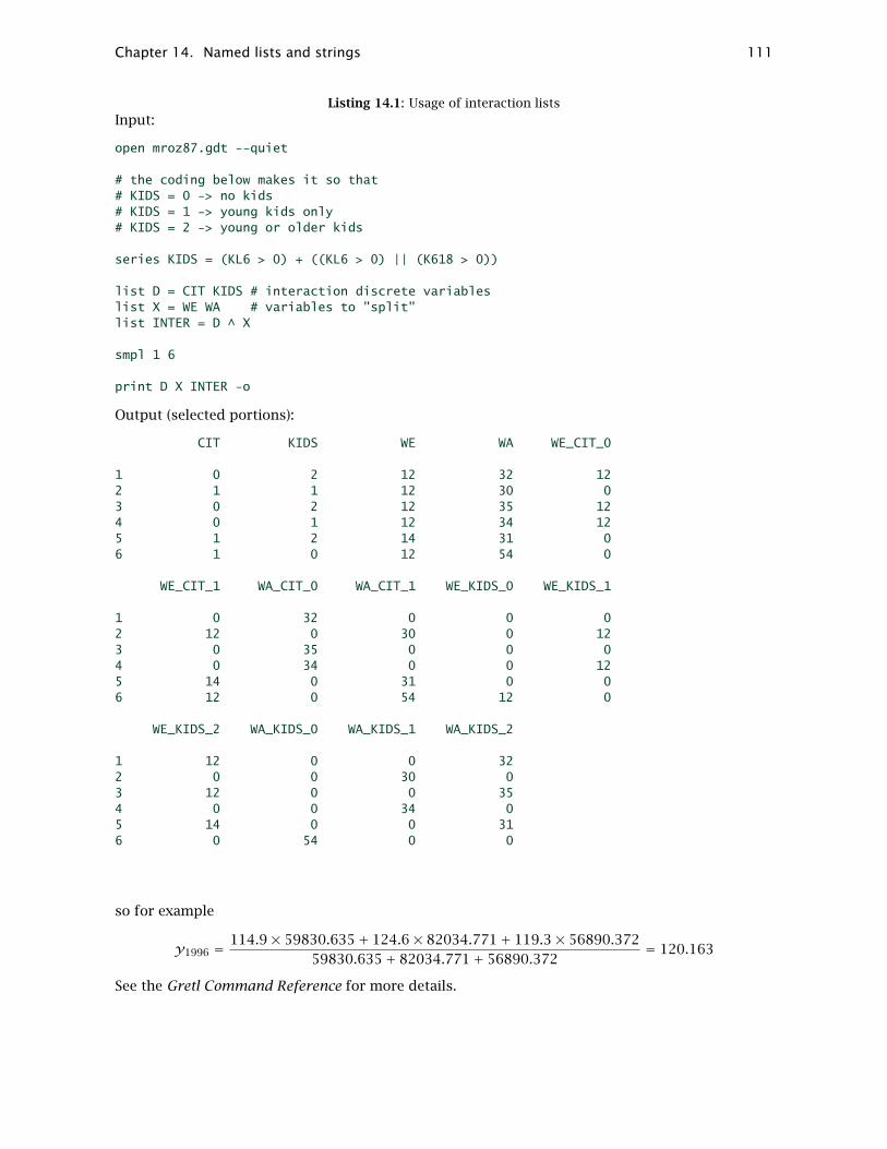
Chapter 14. Named lists and strings 111
Listing 14.1: Usage of interaction listsInput:
open mroz87.gdt --quiet
# the coding below makes it so that# KIDS = 0 -> no kids# KIDS = 1 -> young kids only# KIDS = 2 -> young or older kids
series KIDS = (KL6 > 0) + ((KL6 > 0) || (K618 > 0))
list D = CIT KIDS # interaction discrete variableslist X = WE WA # variables to "split"list INTER = D ^ X
smpl 1 6
print D X INTER -o
Output (selected portions):
CIT KIDS WE WA WE_CIT_0
1 0 2 12 32 122 1 1 12 30 03 0 2 12 35 124 0 1 12 34 125 1 2 14 31 06 1 0 12 54 0
WE_CIT_1 WA_CIT_0 WA_CIT_1 WE_KIDS_0 WE_KIDS_1
1 0 32 0 0 02 12 0 30 0 123 0 35 0 0 04 0 34 0 0 125 14 0 31 0 06 12 0 54 12 0
WE_KIDS_2 WA_KIDS_0 WA_KIDS_1 WA_KIDS_2
1 12 0 0 322 0 0 30 03 12 0 0 354 0 0 34 05 14 0 0 316 0 54 0 0
so for example
y1996 =114.9× 59830.635+ 124.6× 82034.771+ 119.3× 56890.372
59830.635+ 82034.771+ 56890.372= 120.163
See the Gretl Command Reference for more details.

Chapter 14. Named lists and strings 112
YpcFR YpcGE YpcIT NFR NGE NIT
1997 114.9 124.6 119.3 59830.635 82034.771 56890.372
1998 115.3 122.7 120.0 60046.709 82047.195 56906.744
1999 115.0 122.4 117.8 60348.255 82100.243 56916.317
2000 115.6 118.8 117.2 60750.876 82211.508 56942.108
2001 116.0 116.9 118.1 61181.560 82349.925 56977.217
2002 116.3 115.5 112.2 61615.562 82488.495 57157.406
2003 112.1 116.9 111.0 62041.798 82534.176 57604.658
2004 110.3 116.6 106.9 62444.707 82516.260 58175.310
2005 112.4 115.1 105.1 62818.185 82469.422 58607.043
2006 111.9 114.2 103.3 63195.457 82376.451 58941.499
Table 14.1: GDP per capita and population in 3 European countries (Source: Eurostat)
14.2 Named strings
For some purposes it may be useful to save a string (that is, a sequence of characters) as a namedvariable that can be reused.
Some examples of the definition of a string variable are shown below.
string s1 = "some stuff I want to save"string s2 = getenv("HOME")string s3 = s1 + 11
The first field after the type-name string is the name under which the string should be saved, thencomes an equals sign, then comes a specification of the string to be saved. This can be the keywordnull, to produce an empty string, or may take any of the following forms:
• a string literal (enclosed in double quotes); or
• the name of an existing string variable; or
• a function that returns a string (see below); or
• any of the above followed by + and an integer offset.
The role of the integer offset is to use a substring of the preceding element, starting at the givencharacter offset. An empty string is returned if the offset is greater than the length of the string inquestion.
To add to the end of an existing string you can use the operator ~=, as in
string s1 = "some stuff I want to "string s1 ~= "save"
or you can use the ~ operator to join two or more strings, as in
string s1 = "sweet"string s2 = "Home, " ~ s1 ~ " home."
Note that when you define a string variable using a string literal, no characters are treated as“special” (other than the double quotes that delimit the string). Specifically, the backslash is notused as an escape character. So, for example,
Chapter 14. Named lists and strings 113
string s = "\"
is a valid assignment, producing a string that contains a single backslash character. If you wish touse backslash-escapes to denote newlines, tabs, embedded double-quotes and so on, use sprintfinstead.
The sprintf command can also be used to define a string variable. This command works inexactly the same way as the printf command except that the “format” string must be precededby an identifier: either the name of an existing string variable or a new name to which the stringshould be assigned. For example,
scalar x = 8sprintf foo "var%d", x
String variables and string substitution
String variables can be used in two ways in scripting: the name of the variable can be typed “asis”, or it may be preceded by the “at” sign, @. In the first variant the named string is treated as avariable in its own right, while the second calls for “string substitution”. The context determineswhich of these variants is appropriate.
In the following contexts the names of string variables should be given in plain form (without the“at” sign):
• When such a variable appears among the arguments to the commands printf or sprintf.
• When such a variable is given as the argument to a function.
• On the right-hand side of a string assignment.
Here is an illustration of the use of a named string argument with printf:
? string vstr = "variance"Generated string vstr? printf "vstr: %12s\n", vstrvstr: variance
String substitution can be used in contexts where a string variable is not acceptable as such. Ifgretl encounters the symbol @ followed directly by the name of a string variable, this notation istreated as a “macro”: the value of the variable is sustituted literally into the command line beforethe regular parsing of the command is carried out.
One common use of string substitution is when you want to construct and use the name of a seriesprogramatically. For example, suppose you want to create 10 random normal series named norm1to norm10. This can be accomplished as follows.
string sname = nullloop i=1..10sprintf sname "norm%d", iseries @sname = normal()
endloop
Note that plain sname could not be used in the second line within the loop: the effect would beto attempt to overwrite the string variable named sname with a series of the same name. Whatwe want is for the current value of sname to be dumped directly into the command that defines aseries, and the “@” notation achieves that.
Another typical use of string substitution is when you want the options used with a particularcommand to vary depending on some condition. For example,

Chapter 14. Named lists and strings 114
function void use_optstr (series y, list xlist, int verbose)string optstr = verbose ? "" : "--simple-print"ols y xlist @optstr
end function
open data4-1list X = const sqftuse_optstr(price, X, 1)use_optstr(price, X, 0)
When printing the value of a string variable using the print command, the plain variable nameshould generally be used, as in
string s = "Just testing"print s
The following variant is equivalent, though clumsy.
string s = "Just testing"print "@s"
But note that this next variant does something quite different.
string s = "Just testing"print @s
After string substitution, the print command reads
print Just testing
which attempts to print the values of two variables, Just and testing.
Built-in strings
Apart from any strings that the user may define, some string variables are defined by gretl itself.These may be useful for people writing functions that include shell commands. The built-in stringsare as shown in Table 14.2.
gretldir the gretl installation directory
workdir user’s current gretl working directory
dotdir the directory gretl uses for temporary files
gnuplot path to, or name of, the gnuplot executable
tramo path to, or name of, the tramo executable
x12a path to, or name of, the x-12-arima executable
tramodir tramo data directory
x12adir x-12-arima data directory
Table 14.2: Built-in string variables
To access these as ordinary string variables, prepend a dollar sign (as in $dotdir); to use them instring-substitution mode, prepend the at-sign (@dotdir).
Reading strings from the environment
It is possible to read into gretl’s named strings, values that are defined in the external environment.To do this you use the function getenv, which takes the name of an environment variable as itsargument. For example:

Chapter 14. Named lists and strings 115
? string user = getenv("USER")Generated string user? string home = getenv("HOME")Generated string home? printf "%s’s home directory is %s\n", user, homecottrell’s home directory is /home/cottrell
To check whether you got a non-empty value from a given call to getenv, you can use the functionstrlen, which retrieves the length of the string, as in
? string temp = getenv("TEMP")Generated string temp? scalar x = strlen(temp)Generated scalar x = 0
Capturing strings via the shell
If shell commands are enabled in gretl, you can capture the output from such commands using thesyntax
string stringname = $(shellcommand)
That is, you enclose a shell command in parentheses, preceded by a dollar sign.
Reading from a file into a string
You can read the content of a file into a string variable using the syntax
string stringname = readfile(filename)
The filename field may be given as a string variable. For example
? sprintf fname "%s/QNC.rts", $x12adirGenerated string fname? string foo = readfile(fname)Generated string foo
More string functions
Gretl offers several functions for creating or manipulating strings. You can find these listed andexplained in the Function Reference under the category Strings.

Chapter 15
String-valued series
15.1 Introduction
Gretl’s support for data series with string values has gone through three phases:
1. No support: we simply rejected non-numerical values when reading data from file.
2. Numeric encoding only: we would read a string-valued series from a delimited text data file(provided the series didn’t mix numerical values and strings) but the representation of thedata within gretl was purely numerical. We printed a “string table” showing the mappingbetween the original strings and gretl’s encoding and it was up to the user to keep track ofthis mapping.
3. Preservation of string values: the string table that we construct in reading a string-valuedseries is now stored as a component of the dataset so it’s possible to display and manipulatethese values within gretl.
The third phase has now been in effect for several years, with a series of gradual refinements.This chapter gives an account of the status quo. It explains how to create string-valued series anddescribes the operations that are supported for such series.
15.2 Creating a string-valued series
This can be done in two ways: first, by reading such a series from a suitable source file and second,by taking a suitable numerical series within gretl and adding string values using the stringify()function. In either case string values will now be preserved when such a series is saved in a gretl-native data file.
Reading string-valued series
The primary “suitable source” for string-valued series is a delimited text data file (but see sec-tion15.5 below). Here’s a little example. The following is the content of a file named gc.csv:
city,year"Bilbao",2009"Torun",2011"Oklahoma City",2013"Berlin",2015"Athens",2017
and here’s a script:
open gc.csv --quietprint --byobsprint city --byobs --numericprintf "The third gretl conference took place in %s.\n", city[3]
The output from the script is:
116

Chapter 15. String-valued series 117
? print --byobs
city year
1 Bilbao 20092 Torun 20113 Oklahoma C.. 20134 Berlin 20155 Athens 2017
? print city --byobs --numeric
city
1 12 23 34 45 5
The third gretl conference took place in Oklahoma City.
From this we can see a few things.
• By default the print command shows us the string values of the series city, and it han-dles non-ASCII characters provided they’re in UTF-8 (but it doesn’t handle longer strings veryelegantly).
• The --numeric option to print exposes the numeric codes for a string-valued series.
• The syntax seriesname[obs] gives a string when a series is string-valued.
Suppose you want to access the numeric code for a particular string-valued observation: you canget that by “casting” the series to a vector. Thus
printf "The code for ’%s’ is %d.\n", city[3], city[3]
gives
The code for ’Oklahoma City’ is 3.
The numeric codes for string-valued series are always assigned thus: reading the data file row byrow, the first string value is assigned 1, the next distinct string value is assigned 2, and so on.
Assigning string values to an existing series
This is done via the stringify() function, which takes two arguments, the name of a series andan array of strings. For this to work two conditions must be met:
1. The series must have only integer values and the smallest value must be 1 or greater.
2. The array of strings must have at least n members, where n is the largest value found in theseries.
The logic of these conditions is that we’re looking to create a mapping as described above, froma 1-based sequence of integers to a set of strings. However, we’re allowing for the possibility thatthe series in question is an incomplete sample from an associated population. Suppose we have a

Chapter 15. String-valued series 118
series that goes 2, 3, 5, 9, 10. This is taken to be a sample from a population that has at least 10discrete values, 1, 2, . . . , 10, and so requires at least 10 value-strings.
One aspect of stringify() is debatable. At present the function returns 0 on success, otherwisean integer error code; it doesn’t explicitly “fail” if the required conditions are not met, and it’s upto the user to check if things went OK. Maybe it should just fail on error?
Here’s (a simplified version of) an example that one of the authors has had cause to use: derivingUS-style “letter grades” from a series containing percentage scores for students. Call the percentageseries x, and say we want to create a series with values A for x ≥ 90, B for 80 ≤ x < 90, and so ondown to F for x < 60. Then we can do:
series grade = 1 # F, the least valuegrade += x >= 60 # Dgrade += x >= 70 # Cgrade += x >= 80 # Bgrade += x >= 90 # Astringify(grade, strsplit("F D C B A"))
The way the grade series is constructed is not the most compact, but it’s nice and explicit, andeasy to amend if one wants to adjust the threshold values. Note the use of strsplit() to createan on-the-fly array of strings from a string literal; this is convenient when the array contains amoderate number of elements with no embedded spaces. An alternative way to get the same resultis to define the array of strings via the defarray() function, as in
stringify(grade,defarray("F","D","C","B","A"))
We should also mention that we have a function to perform the inverse operation of stringify():the strvals() function retrieves the array of string values from a series. (It returns an empty arrayif the series is not string-valued.)
15.3 Permitted operations
One question that arises with string-valued series is, what are you allowed to do with them andwhat is banned? This may be another debatable point, but here we set out the current state ofthings.
Setting values per observation
You can set particular values in a string-valued series either by string or numeric code. For example,suppose (in relation to the example in section 15.2) that for some reason student number 31 witha percentage score of 88 nonetheless merits an A grade. We could do
grade[31] = "A"
or, if we’re confident about the mapping,
grade[31] = 5
Or to raise the student’s grade by one letter:
grade[31] += 1
What you’re not allowed to do here is make a numerical adjustment that would put the value outof bounds in relation to the set of string values. For example, if we tried grade[31] = 6 we’d getan error.

Chapter 15. String-valued series 119
On the other hand, you can implicitly extend the set of string values. This wouldn’t make sense forthe letter grades example but it might for, say, city names. Returning to the example in section 15.2suppose we try
dataset addobs 1year[6] = 2019city[6] = "Naples?"
This will work OK: we’re implicitly adding another member to the string table for city; the associ-ated numeric code will be the next available integer.1
Assignment to an entire series
This is disallowed: you can’t execute an assignment of any sort with the name of a string-valuedseries per se on the left-hand side. Put differently, you cannot overwrite an entire string-valuedseries at once. This may be debatable, but it’s much the easiest way of ensuring that we never endup with a broken mapping. If anyone can come up with a really good reason for wanting to do thiswe might reconsider.
Besides assigning an out-of-bounds numerical value to a particular observation, this sort of assign-ment is in fact the only operation that is banned for string-valued series.
Missing values
We support one exception to the general rule, never break the mapping between strings and nu-meric codes for string-valued series: you can mark particular observations as missing. This is donein the usual way, e.g.,
grade[31] = NA
Note, however, that on importing a string series from a delimited text file any non-blank strings (in-cluding “NA”) will be interpreted as valid values; any missing values in such a file should thereforebe represented by blank cells.
Copying a string-valued series
If you make a copy of a string-valued series, as in
series foo = city
the string values are not copied over: you get a purely numerical series holding the codes of theoriginal series. But if you want a full copy with the string values that can easily be arranged:
series citycopy = citystringify(citycopy, strvals(city))
String-valued series in other contexts
String-valued series can be used on the right-hand side of assignment statements at will, and inthat context their numerical values are taken. For example,
series y = sqrt(city)
1Admittedly there is a downside to this feature: one may inadvertently add a new string value by mistyping a stringthat’s already present.

Chapter 15. String-valued series 120
will elicit no complaint and generate a numerical series 1, 1.41421, . . . . It’s up to the user to judgewhether this sort of thing makes any sense.
Similarly, it’s up to the user to decide if it makes sense to use a string-valued series “as is” in aregression model, whether as regressand or regressor—again, the numerical values of the seriesare taken. Often this will not make sense, but sometimes it may: the numerical values may bydesign form an ordinal, or even a cardinal, scale (as in the “grade” example in section 15.2).
More likely, one would want to use dummify on a string-valued series before using it in statisticalmodeling. In that context gretl’s series labels are suitably informative. For example, suppose wehave a series race with numerical values 1, 2 and 3 and associated strings “White”, “Black” and“Other”. Then the hansl code
list D = dummify(race)labels
will show these labels:
Drace_2: dummy for race = ’Black’Drace_3: dummy for race = ’Other’
Given such a series you can use string values in a sample restriction, as in
smpl race == "Black" --restrict
(although race == 2 would also be acceptable).
There may be other contexts that we haven’t yet thought of where it would be good to have stringvalues displayed and/or accepted on input; suggestions are welcome.
15.4 String-valued series and functions
User-defined hansl functions can deal with string-valued series, although there are a few points tonote.
If you supply such a series as an argument to a hansl function its string values will be accessiblewithin the function. One can test whether a given series arg is string-valued as follows:
if nelem(strvals(arg)) > 0# yes
else# no
endif
Now suppose one wanted to put something like the code that generated the grade series in sec-tion 15.2 into a function. That can be done, but not in the form of a function that directly returnsthe desired series—that is, something like
function series letter_grade (series x)series grade# define grade based on x and stringify it, as shown abovereturn grade
end function
Unfortunately the above will not work: the caller will get the grade series OK but it won’t be string-valued. At first sight this may seem to be a bug but it’s defensible as a consequence of the wayseries work in gretl.

Chapter 15. String-valued series 121
The point is that series have, so to speak, two grades of existence. They can exist as fully-fledgedmembers of a dataset, or they can have a fleeting existence as simply anonymous arrays of numbersthat are of the same length as dataset series. Consider the statement
series rootx1 = sqrt(x+1)
On the right-hand side we have the “series” x+1, which is called into existence as part of a calcula-tion but has no name and cannot have string values. Similarly, consider
series grade = letter_grade(x)
The return value from letter_grade() is likewise an anonymous array,2 incapable of holdingstring values until it gets assigned to the named series grade. The solution is to define grade as aseries, at the level of the caller, before calling letter_grade(), as in
function void letter_grade (series x, series *grade)# define grade based on x and stringify it# this version will work!
end function
# caller...series gradeletter_grade(x, &grade)
As you’ll see from the account above, we don’t offer any very fancy facilities for string-valuedseries. We’ll read them from suitable sources and we’ll create them natively via stringify—andwe’ll try to ensure that they retain their integrity—but we don’t, for example, take the specificationof a string-valued series as a regressor as an implicit request to include the dummification of itsdistinct values. Besides laziness, this reflects the fact that in gretl a string-valued series may beusable “as is”, depending on how it’s defined; you can use dummify if you need it.
15.5 Other import formats
In section 15.2 we illustrated the reading of string-valued series with reference to a delimited textdata file. Gretl can also handle several other sources of string-valued data, including the spread-sheet formats xls, xlsx, gnumeric and ods and (to a degree) the formats of Stata, SAS and SPSS.
Stata files
Stata supports two relevant sorts of variables: (1) those that are of “string type” and (2) variablesof one or other numeric type that have “value labels” defined. Neither of these is exactly equivalentto what we call a “string-valued series” in gretl.
Stata variables of string type have no numeric representation; their values are literally strings, andthat’s all. Stata’s numeric variables with value labels do not have to be integer-valued and theirleast value does not have to be 1; however, you can’t define a label for a value that is not an integer.Thus in Stata you can have a series that comprises both integer and non-integer values, but onlythe integer values can be labeled.3
This means that on import to gretl we can readily handle variables of string type from Stata’s dtafiles. We give them a 1-based numeric encoding; this is arbitrary but does not conflict with anyinformation in the dta file. On the other hand, in general we’re not able to handle Stata’s numeric
2A proper named series, with string values, existed while the function was executing but it ceased to exist as soon asthe function was finished.
3Verified in Stata 12.

Chapter 15. String-valued series 122
variables with value labels; currently we report the value labels to the user but do not attempt tostore them in the gretl dataset. We could check such variables and import them as string-valuedseries if they satisfy the criteria stated in section 15.2 but we don’t at present.
SAS and SPSS files
Gretl is able to read and preserve string values associated with variables from SAS “export” (xpt)files, and also from SPSS sav files. Such variables seem to be on the same pattern as Stata variablesof string type.

Chapter 16
Matrix manipulation
Together with the other two basic types of data (series and scalars), gretl offers a quite compre-hensive array of matrix methods. This chapter illustrates the peculiarities of matrix syntax anddiscusses briefly some of the more complex matrix functions. For a full listing of matrix functionsand a comprehensive account of their syntax, please refer to the Gretl Command Reference.
16.1 Creating matrices
Matrices can be created using any of these methods:
1. By direct specification of the scalar values that compose the matrix — in numerical form, byreference to pre-existing scalar variables, or using computed values.
2. By providing a list of data series.
3. By providing a named list of series.
4. Using a formula of the same general type that is used with the genr command, whereby a newmatrix is defined in terms of existing matrices and/or scalars, or via some special functions.
To specify a matrix directly in terms of scalars, the syntax is, for example:
matrix A = 1, 2, 3 ; 4, 5, 6
The matrix is defined by rows; the elements on each row are separated by commas and the rowsare separated by semi-colons. The whole expression must be wrapped in braces. Spaces within thebraces are not significant. The above expression defines a 2 × 3 matrix. Each element should be anumerical value, the name of a scalar variable, or an expression that evaluates to a scalar. Directlyafter the closing brace you can append a single quote (’) to obtain the transpose.
To specify a matrix in terms of data series the syntax is, for example,
matrix A = x1, x2, x3
where the names of the variables are separated by commas. Besides names of existing variables,you can use expressions that evaluate to a series. For example, given a series x you could do
matrix A = x, x^2
Each variable occupies a column (and there can only be one variable per column). You cannot usethe semicolon as a row separator in this case: if you want the series arranged in rows, append thetranspose symbol. The range of data values included in the matrix depends on the current settingof the sample range.
Instead of giving an explicit list of variables, you may instead provide the name of a saved list (seeChapter 14), as in
123

Chapter 16. Matrix manipulation 124
list xlist = x1 x2 x3matrix A = xlist
When you provide a named list, the data series are by default placed in columns, as is natural in aneconometric context: if you want them in rows, append the transpose symbol.
As a special case of constructing a matrix from a list of variables, you can say
matrix A = dataset
This builds a matrix using all the series in the current dataset, apart from the constant (variable 0).When this dummy list is used, it must be the sole element in the matrix definition .... You can,however, create a matrix that includes the constant along with all other variables using horizontalconcatenation (see below), as in
matrix A = const~dataset
By default, when you build a matrix from series that include missing values the data rows thatcontain NAs are skipped. But you can modify this behavior via the command set skip_missingoff. In that case NAs are converted to NaN (“Not a Number”). In the IEEE floating-point stan-dard, arithmetic operations involving NaN always produce NaN. Alternatively, you can take greatercontrol over the observations (data rows) that are included in the matrix using the “set” variablematrix_mask, as in
set matrix_mask msk
where msk is the name of a series. Subsequent commands that form matrices from series or lists willinclude only observations for which msk has non-zero (and non-missing) values. You can removethis mask via the command set matrix_mask null.
+ Names of matrices must satisfy the same requirements as names of gretl variables in general: the namecan be no longer than 31 characters, must start with a letter, and must be composed of nothing but letters,numbers and the underscore character.
16.2 Empty matrices
The syntax
matrix A =
creates an empty matrix—a matrix with zero rows and zero columns.
The main purpose of the concept of an empty matrix is to enable the user to define a starting pointfor subsequent concatenation operations. For instance, if X is an already defined matrix of any size,the commands
matrix A = matrix B = A ~ X
result in a matrix B identical to X.
From an algebraic point of view, one can make sense of the idea of an empty matrix in terms ofvector spaces: if a matrix is an ordered set of vectors, then A= is the empty set. As a consequence,operations involving addition and multiplications don’t have any clear meaning (arguably, they havenone at all), but operations involving the cardinality of this set (that is, the dimension of the spacespanned by A) are meaningful.

Chapter 16. Matrix manipulation 125
Function Return value Function Return value
A’, transp(A) A rows(A) 0
cols(A) 0 rank(A) 0
det(A) NA ldet(A) NA
tr(A) NA onenorm(A) NA
infnorm(A) NA rcond(A) NA
Table 16.1: Valid functions on an empty matrix, A
Legal operations on empty matrices are listed in Table 16.1. (All other matrix operations gener-ate an error when an empty matrix is given as an argument.) In line with the above interpreta-tion, some matrix functions return an empty matrix under certain conditions: the functions diag,vec, vech, unvech when the arguments is an empty matrix; the functions I, ones, zeros,mnormal, muniform when one or more of the arguments is 0; and the function nullspace whenits argument has full column rank.
16.3 Selecting sub-matrices
You can select sub-matrices of a given matrix using the syntax
A[rows,cols]
where rows can take any of these forms:
1. empty selects all rows
2. a single integer selects the single specified row
3. two integers separated by a colon selects a range of rows
4. the name of a matrix selects the specified rows
With regard to option 2, the integer value can be given numerically, as the name of an existingscalar variable, or as an expression that evaluates to a scalar. With option 4, the index matrix givenin the rows field must be either p × 1 or 1× p, and should contain integer values in the range 1 ton, where n is the number of rows in the matrix from which the selection is to be made.
The cols specification works in the same way, mutatis mutandis. Here are some examples.
matrix B = A[1,]matrix B = A[2:3,3:5]matrix B = A[2,2]matrix idx = 1, 2, 6matrix B = A[idx,]
The first example selects row 1 from matrix A; the second selects a 2×3 submatrix; the third selectsa scalar; and the fourth selects rows 1, 2, and 6 from matrix A.
If the matrix in question is n × 1 or 1 ×m, it is OK to give just one index specifier and omit thecomma. For example, A[2] selects the second element of A if A is a vector. Otherwise the commais mandatory.
In addition there is a pre-defined index specification, diag, which selects the principal diagonal ofa square matrix, as in B[diag], where B is square.
You can use selections of this sort on either the right-hand side of a matrix-generating formula orthe left. Here is an example of use of a selection on the right, to extract a 2× 2 submatrix B from a3× 3 matrix A:

Chapter 16. Matrix manipulation 126
matrix A = 1, 2, 3; 4, 5, 6; 7, 8, 9matrix B = A[1:2,2:3]
And here are examples of selection on the left. The second line below writes a 2×2 identity matrixinto the bottom right corner of the 3× 3 matrix A. The fourth line replaces the diagonal of A with1s.
matrix A = 1, 2, 3; 4, 5, 6; 7, 8, 9matrix A[2:3,2:3] = I(2)matrix d = 1, 1, 1matrix A[diag] = d
16.4 Deleting rows or columns
A variant of sub-matrix notation is available for convenience in dropping specified rows and/orcolumns from a matrix, namely giving negative values for the indices. Here is a simple example,
matrix A = 1, 2, 3; 4, 5, 6; 7, 8, 9matrix B = A[-2,-3]
which creates B as a 2×2 matrix which drops row 2 and column 3 from A. Negative indices can alsobe given in the form of an index vector:
matrix rdrop = -1,-3,-5matrix B = A[rdrop,]
In this case B is formed by dropping rows 1, 3 and 5 from A (which must have at least 5 rows), butretaining the column dimension of A.
There are two limitations on the use of negative indices. First, the from:to range syntax describedin the previous section is not available, but you can use the seq function to achieve an equivalenteffect, as in
matrix A = muniform(1, 10)matrix B = A[,-seq(3,7)]
where B drops columns 3 to 7 from A. Second, use of negative indices is valid only on the right-handside of a matrix calculation; there is no “negative index” equivalent of assignment to a sub-matrix,as in
A[1:3,] = ones(3, cols(A))
16.5 Matrix operators
The following binary operators are available for matrices:

Chapter 16. Matrix manipulation 127
+ addition
- subtraction
* ordinary matrix multiplication
’ pre-multiplication by transpose
\ matrix “left division” (see below)
/ matrix “right division” (see below)
~ column-wise concatenation
| row-wise concatenation
** Kronecker product
== test for equality
!= test for inequality
In addition, the following operators (“dot” operators) apply on an element-by-element basis:
.+ .- .* ./ .^ .= .> .< .>= .<= .!=
Here are explanations of the less obvious cases.
For matrix addition and subtraction, in general the two matrices have to be of the same dimensionsbut an exception to this rule is granted if one of the operands is a 1×1 matrix or scalar. The scalaris implicitly promoted to the status of a matrix of the correct dimensions, all of whose elementsare equal to the given scalar value. For example, if A is an m × n matrix and k a scalar, then thecommands
matrix C = A + kmatrix D = A - k
both produce m×n matrices, with elements cij = aij + k and dij = aij − k respectively.
By “pre-multiplication by transpose” we mean, for example, that
matrix C = X’Y
produces the product of X-transpose and Y . In effect, the expression X’Y is shorthand for X’*Y,which is also valid. Consider, however, that in the special case X = Y , the two are not exactlyequivalent: the former expression uses a specialized, optimized algorithm which has the doubleadvantage of being more efficient computationally and of ensuring that the result will be free byconstruction of machine precision artifacts that may render it numerically non-symmetric. This,however, is unlikely to affect you unless your X matrix is rather large (at least several hundredsrows/columns).
In matrix “left division”, the statement
matrix X = A \ B
is interpreted as a request to find the matrix X that solves AX = B. If B is a square matrix, this isin principle equivalent to A−1B, which fails if A is singular; the numerical method employed hereis the LU decomposition. If A is a T × k matrix with T > k, then X is the least-squares solution,X = (A′A)−1A′B, which fails if A′A is singular; the numerical method employed here is the QRdecomposition. Otherwise, the operation necessarily fails.
For matrix “right division”, as in X = A / B, X is the matrix that solves XB = A, in principleequivalent to AB−1.
In “dot” operations a binary operation is applied element by element; the result of this operationis obvious if the matrices are of the same size. However, there are several other cases where suchoperators may be applied. For example, if we write

Chapter 16. Matrix manipulation 128
matrix C = A .- B
then the result C depends on the dimensions of A and B. Let A be an m × n matrix and let B bep × q; the result is as follows:
Case Result
Dimensions match (m = p and n = q) cij = aij − bijA is a column vector; rows match (m = p; n = 1) cij = ai − bijB is a column vector; rows match (m = p; q = 1) cij = aij − biA is a row vector; columns match (m = 1; n = q) cij = aj − bijB is a row vector; columns match (m = p; q = 1) cij = aij − bjA is a column vector; B is a row vector (n = 1; p = 1) cij = ai − bjA is a row vector; B is a column vector (m = 1; q = 1) cij = aj − biA is a scalar (m = 1 and n = 1) cij = a− bijB is a scalar (p = 1 and q = 1) cij = aij − b
If none of the above conditions are satisfied the result is undefined and an error is flagged.
Note that this convention makes it unnecessary, in most cases, to use diagonal matrices to performtransformations by means of ordinary matrix multiplication: if Y = XV , where V is diagonal, it iscomputationally much more convenient to obtain Y via the instruction
matrix Y = X .* v
where v is a row vector containing the diagonal of V .
In column-wise concatenation of anm×nmatrix A and anm×pmatrix B, the result is anm×(n+p)matrix. That is,
matrix C = A ~ B
produces C =[A B
].
Row-wise concatenation of an m × n matrix A and an p × n matrix B produces an (m + p) × nmatrix. That is,
matrix C = A | B
produces C =[AB
].
16.6 Matrix–scalar operators
For matrix A and scalar k, the operators shown in Table 16.2 are available. (Addition and subtrac-tion were discussed in section 16.5 but we include them in the table for completeness.) In addition,for square A and integer k ≥ 0, B = A^k produces a matrix B which is A raised to the power k.
16.7 Matrix functions
Most of the gretl functions available for scalars and series also apply to matrices in an element-by-element fashion, and as such their behavior should be pretty obvious. This is the case for functionssuch as log, exp, sin, etc. These functions have the effects documented in relation to the genrcommand. For example, if a matrix A is already defined, then

Chapter 16. Matrix manipulation 129
Expression Effect
matrix B = A * k bij = kaijmatrix B = A / k bij = aij/kmatrix B = k / A bij = k/aijmatrix B = A + k bij = aij + kmatrix B = A - k bij = aij − kmatrix B = k - A bij = k− aijmatrix B = A % k bij = aij modulo k
Table 16.2: Matrix–scalar operators
matrix B = sqrt(A)
generates a matrix such that bij = √aij . All such functions require a single matrix as argument, oran expression which evaluates to a single matrix.1
In this section, we review some aspects of genr functions that apply specifically to matrices. A fullaccount of each function is available in the Gretl Command Reference.
Matrix reshaping
In addition to the methods discussed in sections 16.1 and 16.3, a matrix can also be created byre-arranging the elements of a pre-existing matrix. This is accomplished via the mshape function.It takes three arguments: the input matrix, A, and the rows and columns of the target matrix, rand c respectively. Elements are read from A and written to the target in column-major order. If Acontains fewer elements than n = r × c, they are repeated cyclically; if A has more elements, onlythe first n are used.
For example:
matrix a = mnormal(2,3)amatrix b = mshape(a,3,1)bmatrix b = mshape(a,5,2)b
produces
? aa
1.2323 0.99714 -0.390780.54363 0.43928 -0.48467
? matrix b = mshape(a,3,1)Generated matrix b? bb
1.23230.54363
1Note that to find the “matrix square root” you need the cholesky function (see below); moreover, the exp functioncomputes the exponential element by element, and therefore does not return the matrix exponential unless the matrix isdiagonal—to get the matrix exponential, use mexp.

Chapter 16. Matrix manipulation 130
Creation and I/Odiag diagcat I lower mnormal mread
muniform mwrite ones seq unvech upper
vec vech zeros
Shape/size/arrangementcols dsort mreverse mshape msortby rows
selifc selifr sort trimr
Matrix algebracdiv cholesky cmult cnumber det eigengen
eigensym eigsolve fft ffti ginv hdprod
infnorm inv invpd ldet mexp nullspace
onenorm polroots psdroot qform qrdecomp rank
rcond svd toepsolv tr transp varsimul
Statistics/transformationsaggregate cdemean corr corrgm cov ecdf
fcstats ghk gini halton imaxc imaxr
iminc iminr irf iwishart kdensity kmeier
kpsscrit maxc maxr mcorr mcov mcovg
meanc meanr minc minr mlag mols
mpols mrls mxtab naalen normtest npcorr
pergm princomp prodc prodr quadtable quantile
ranking resample sdc sumc sumr uniq
values
Numerical methodsBFGSmax BFGScmax fdjac GSSmax NMmax NRmax
simann
Decorationcolnames rownames
Table 16.3: Matrix functions by category

Chapter 16. Matrix manipulation 131
0.99714
? matrix b = mshape(a,5,2)Replaced matrix b? bb
1.2323 -0.484670.54363 1.23230.99714 0.543630.43928 0.99714
-0.39078 0.43928
Complex multiplication and division
Gretl has no native provision for complex numbers. However, basic operations can be performedon vectors of complex numbers by using the convention that a vector of n complex numbers isrepresented as a n × 2 matrix, where the first column contains the real part and the second theimaginary part.
Addition and subtraction are trivial; the functions cmult and cdiv compute the complex productand division, respectively, of two input matrices, A and B, representing complex numbers. Thesematrices must have the same number of rows, n, and either one or two columns. The first columncontains the real part and the second (if present) the imaginary part. The return value is an n × 2matrix, or, if the result has no imaginary part, an n-vector.
For example, suppose you have z1 = [1+ 2i,3+ 4i]′ and z2 = [1, i]′:
? z1 = 1,2;3,4z1 = 1,2;3,4
Generated matrix z1? z2 = I(2)z2 = I(2)
Generated matrix z2? conj_z1 = z1 .* 1,-1conj_z1 = z1 .* 1,-1
Generated matrix conj_z1? eval cmult(z1,z2)eval cmult(z1,z2)1 2
-4 3
? eval cmult(z1,conj_z1)eval cmult(z1,conj_z1)5
25
Multiple returns and the null keyword
Some functions take one or more matrices as arguments and compute one or more matrices; theseare:
eigensym Eigen-analysis of symmetric matrix
eigengen Eigen-analysis of general matrix
mols Matrix OLS
qrdecomp QR decomposition
svd Singular value decomposition (SVD)

Chapter 16. Matrix manipulation 132
The general rule is: the “main” result of the function is always returned as the result proper.Auxiliary returns, if needed, are retrieved using pre-existing matrices, which are passed to thefunction as pointers (see 13.4). If such values are not needed, the pointer may be substituted withthe keyword null.
The syntax for qrdecomp, eigensym and eigengen is of the form
matrix B = func(A, &C)
The first argument, A, represents the input data, that is, the matrix whose decomposition or analysisis required. The second argument must be either the name of an existing matrix preceded by & (toindicate the “address” of the matrix in question), in which case an auxiliary result is written to thatmatrix, or the keyword null, in which case the auxiliary result is not produced, or is discarded.
In case a non-null second argument is given, the specified matrix will be over-written with theauxiliary result. (It is not required that the existing matrix be of the right dimensions to receive theresult.)
The function eigensym computes the eigenvalues, and optionally the right eigenvectors, of a sym-metric n × n matrix. The eigenvalues are returned directly in a column vector of length n; if theeigenvectors are required, they are returned in an n×n matrix. For example:
matrix Vmatrix E = eigensym(M, &V)matrix E = eigensym(M, null)
In the first case E holds the eigenvalues of M and V holds the eigenvectors. In the second, E holdsthe eigenvalues but the eigenvectors are not computed.
The function eigengen computes the eigenvalues, and optionally the eigenvectors, of a generaln×n matrix. The eigenvalues are returned directly in an n×2 matrix, the first column holding thereal components and the second column the imaginary components.
If the eigenvectors are required (that is, if the second argument to eigengen is not null), theyare returned in an n × n matrix. The column arrangement of this matrix is somewhat non-trivial:the eigenvectors are stored in the same order as the eigenvalues, but the real eigenvectors occupyone column, whereas complex eigenvectors take two (the real part comes first); the total number ofcolumns is still n, because the conjugate eigenvector is skipped. Listing 16.1 provides a (hopefully)clarifying example (see also subsection 16.7).
The qrdecomp function computes the QR decomposition of an m × n matrix A: A = QR, where Qis anm×n orthogonal matrix and R is an n×n upper triangular matrix. The matrix Q is returneddirectly, while R can be retrieved via the second argument. Here are two examples:
matrix Rmatrix Q = qrdecomp(M, &R)matrix Q = qrdecomp(M, null)
In the first example, the triangular R is saved as R; in the second, R is discarded. The first lineabove shows an example of a “simple declaration” of a matrix: R is declared to be a matrix variablebut is not given any explicit value. In this case the variable is initialized as a 1 × 1 matrix whosesingle element equals zero.
The syntax for svd is
matrix B = func(A, &C, &D)
The function svd computes all or part of the singular value decomposition of the realm×nmatrixA. Let k =min(m,n). The decomposition is
A = UΣV ′
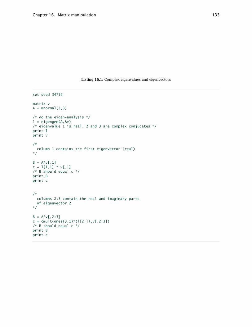
Chapter 16. Matrix manipulation 133
Listing 16.1: Complex eigenvalues and eigenvectors
set seed 34756
matrix vA = mnormal(3,3)
/* do the eigen-analysis */l = eigengen(A,&v)/* eigenvalue 1 is real, 2 and 3 are complex conjugates */print lprint v
/*column 1 contains the first eigenvector (real)
*/
B = A*v[,1]c = l[1,1] * v[,1]/* B should equal c */print Bprint c
/*columns 2:3 contain the real and imaginary partsof eigenvector 2
*/
B = A*v[,2:3]c = cmult(ones(3,1)*(l[2,]),v[,2:3])/* B should equal c */print Bprint c

Chapter 16. Matrix manipulation 134
where U is anm×k orthogonal matrix, Σ is an k×k diagonal matrix, and V is an k×n orthogonalmatrix.2 The diagonal elements of Σ are the singular values of A; they are real and non-negative,and are returned in descending order. The first k columns of U and V are the left and right singularvectors of A.
The svd function returns the singular values, in a vector of length k. The left and/or right singu-lar vectors may be obtained by supplying non-null values for the second and/or third argumentsrespectively. For example:
matrix s = svd(A, &U, &V)matrix s = svd(A, null, null)matrix s = svd(A, null, &V)
In the first case both sets of singular vectors are obtained, in the second case only the singularvalues are obtained; and in the third, the right singular vectors are obtained but U is not computed.Please note: when the third argument is non-null, it is actually V ′ that is provided. To reconstitutethe original matrix from its SVD, one can do:
matrix s = svd(A, &U, &V)matrix B = (U.*s)*V
Finally, the syntax for mols is
matrix B = mols(Y, X, &U)
This function returns the OLS estimates obtained by regressing the T × n matrix Y on the T × kmatrix X, that is, a k × n matrix holding (X′X)−1X′Y . The Cholesky decomposition is used. Thematrix U , if not null, is used to store the residuals.
Reading and writing matrices from/to text files
The two functions mread and mwrite can be used for basic matrix input/output. This can be usefulto enable gretl to exchange data with other programs.
The mread function accepts one string parameter: the name of the (plain text) file from which thematrix is to be read. The file in question may start with any number of comment lines, definedas lines that start with the hash mark, “#”; such lines are ignored. Beyond that, the content mustconform to the following rules:
1. The first non-comment line must contain two integers, separated by a space or a tab, indicat-ing the number of rows and columns, respectively.
2. The columns must be separated by spaces or tab characters.
3. The decimal separator must be the dot “.” character.
Should an error occur (such as the file being badly formatted or inaccessible), an empty matrix (seesection 16.2) is returned.
The complementary function mwrite produces text files formatted as described above. The columnseparator is the tab character, so import into spreadsheets should be straightforward. Usage isillustrated in example 16.2. Matrices stored via the mwrite command can be easily read by otherprograms; the following table summarizes the appropriate commands for reading a matrix A froma file called a.mat in some widely-used programs.3 Note that the Python example requires that thenumpy module is loaded.
2This is not the only definition of the SVD: some writers define U as m ×m, Σ as m × n (with k non-zero diagonalelements) and V as n×n.
3Matlab users may find the Octave example helpful, since the two programs are mostly compatible with one another.

Chapter 16. Matrix manipulation 135
Program Sample code
GAUSS tmp[] = load a.mat;
A = reshape(tmp[3:rows(tmp)],tmp[1],tmp[2]);
Octave fd = fopen("a.mat");
[r,c] = fscanf(fd, "%d %d", "C");
A = reshape(fscanf(fd, "%g", r*c),c,r)’;
fclose(fd);
Ox decl A = loadmat("a.mat");
R A <- as.matrix(read.table("a.mat", skip=1))
Python A = numpy.loadtxt(’a.mat’, skiprows=1)
Julia A = readdlm("a.mat", skipstart=1)
Listing 16.2: Matrix input/output via text files
nulldata 64scalar n = 3string f1 = "a.csv"string f2 = "b.csv"
matrix a = mnormal(n,n)matrix b = inv(a)
err = mwrite(a, f1)
if err != 0fprintf "Failed to write %s\n", f1
elseerr = mwrite(b, f2)
endif
if err != 0fprintf "Failed to write %s\n", f2
elsec = mread(f1)d = mread(f2)a = c*dprintf "The following matrix should be an identity matrix\n"print a
endif
Optionally, the mwrite and mread functions can use gzip compression: this is invoked if the nameof the matrix file has the suffix “.gz.” In this case the elements of the matrix are written in a singlecolumn. Note, however, that compression should not be applied when writing matrices for readingby third-party software unless you are sure that the software can handle compressed data.
16.8 Matrix accessors
In addition to the matrix functions discussed above, various “accessor” strings allow you to createcopies of internal matrices associated with models previously estimated. These are set out inTable 16.4.

Chapter 16. Matrix manipulation 136
$coeff matrix of estimated coefficients
$compan companion matrix (after VAR or VECM estimation)
$jalpha matrix α (loadings) from Johansen’s procedure
$jbeta matrix β (cointegration vectors) from Johansen’s procedure
$jvbeta covariance matrix for the unrestricted elements of β from Johansen’s procedure
$rho autoregressive coefficients for error process
$sigma residual covariance matrix
$stderr matrix of estimated standard errors
$uhat matrix of residuals
$vcv covariance matrix of parameter estimates
$vma VMA matrices in stacked form (see section 29.2)
$yhat matrix of fitted values
Table 16.4: Matrix accessors for model data
Many of the accessors in Table 16.4 behave somewhat differently depending on the sort of modelthat is referenced, as follows:
• Single-equation models: $sigma gets a scalar (the standard error of the regression); $coeffand $stderr get column vectors; $uhat and $yhat get series.
• System estimators: $sigma gets the cross-equation residual covariance matrix; $uhat and$yhat get matrices with one column per equation. The format of $coeff and $stderr de-pends on the nature of the system: for VARs and VECMs (where the matrix of regressors isthe same for all equations) these return matrices with one column per equation, but for othersystem estimators they return a big column vector.
• VARs and VECMs: $vcv is not available, but X′X−1 (where X is the common matrix of regres-sors) is available as $xtxinv.
If the accessors are given without any prefix, they retrieve results from the last model estimated, ifany. Alternatively, they may be prefixed with the name of a saved model plus a period (.), in whichcase they retrieve results from the specified model. Here are some examples:
matrix u = $uhatmatrix b = m1.$coeffmatrix v2 = m1.$vcv[1:2,1:2]
The first command grabs the residuals from the last model; the second grabs the coefficient vectorfrom model m1; and the third (which uses the mechanism of sub-matrix selection described above)grabs a portion of the covariance matrix from model m1.
If the model in question a VAR or VECM (only) $compan and $vma return the companion matrix andthe VMA matrices in stacked form, respectively (see section 29.2 for details). After a vector errorcorrection model is estimated via Johansen’s procedure, the matrices $jalpha and $jbeta are alsoavailable. These have a number of columns equal to the chosen cointegration rank; therefore, theproduct
matrix Pi = $jalpha * $jbeta’
returns the reduced-rank estimate of A(1). Since β is automatically identified via the Phillips nor-malization (see section 30.5), its unrestricted elements do have a proper covariance matrix, whichcan be retrieved through the $jvbeta accessor.

Chapter 16. Matrix manipulation 137
16.9 Namespace issues
Matrices share a common namespace with data series and scalar variables. In other words, no twoobjects of any of these types can have the same name. It is an error to attempt to change the typeof an existing variable, for example:
scalar x = 3matrix x = ones(2,2) # wrong!
It is possible, however, to delete or rename an existing variable then reuse the name for a variableof a different type:
scalar x = 3delete xmatrix x = ones(2,2) # OK
16.10 Creating a data series from a matrix
Section 16.1 above describes how to create a matrix from a data series or set of series. You maysometimes wish to go in the opposite direction, that is, to copy values from a matrix into a regulardata series. The syntax for this operation is
series sname = mspec
where sname is the name of the series to create and mspec is the name of the matrix to copy from,possibly followed by a matrix selection expression. Here are two examples.
series s = xseries u1 = U[,1]
It is assumed that x and U are pre-existing matrices. In the second example the series u1 is formedfrom the first column of the matrix U.
For this operation to work, the matrix (or matrix selection) must be a vector with length equal toeither the full length of the current dataset, n, or the length of the current sample range, n′. Ifn′ < n then only n′ elements are drawn from the matrix; if the matrix or selection comprises nelements, the n′ values starting at element t1 are used, where t1 represents the starting observationof the sample range. Any values in the series that are not assigned from the matrix are set to themissing code.
16.11 Matrices and lists
To facilitate the manipulation of named lists of variables (see Chapter 14), it is possible to convertbetween matrices and lists. In section 16.1 above we mentioned the facility for creating a matrixfrom a list of variables, as in
matrix M = listname
That formulation, with the name of the list enclosed in braces, builds a matrix whose columns holdthe variables referenced in the list. What we are now describing is a different matter: if we say
matrix M = listname
(without the braces), we get a row vector whose elements are the ID numbers of the variables in thelist. This special case of matrix generation cannot be embedded in a compound expression. Thesyntax must be as shown above, namely simple assignment of a list to a matrix.
To go in the other direction, you can include a matrix on the right-hand side of an expression thatdefines a list, as in

Chapter 16. Matrix manipulation 138
list Xl = M
where M is a matrix. The matrix must be suitable for conversion; that is, it must be a row or columnvector containing non-negative integer values, none of which exceeds the highest ID number of aseries in the current dataset.
Listing 16.3 illustrates the use of this sort of conversion to “normalize” a list, moving the constant(variable 0) to first position.
Listing 16.3: Manipulating a list
function void normalize_list (matrix *x)# If the matrix (representing a list) contains var 0,# but not in first position, move it to first position
if (x[1] != 0)scalar k = cols(x)loop for (i=2; i<=k; i++) --quiet
if (x[i] == 0)x[i] == x[1]x[1] == 0break
endifendloop
endifend function
open data9-7list Xl = 2 3 0 4matrix x = Xlnormalize_list(&x)list Xl = x
16.12 Deleting a matrix
To delete a matrix, just write
delete M
where M is the name of the matrix to be deleted.
16.13 Printing a matrix
To print a matrix, the easiest way is to give the name of the matrix in question on a line by itself,which is equivalent to using the print command:
matrix M = mnormal(100,2)Mprint M
You can get finer control on the formatting of output by using the printf command, as illustratedin the interactive session below:

Chapter 16. Matrix manipulation 139
? matrix Id = I(2)matrix Id = I(2)
Generated matrix Id? print Idprint Id
Id (2 x 2)
1 00 1
? printf "%10.3f", Id1.000 0.0000.000 1.000
For presentation purposes you may wish to give titles to the columns of a matrix. For this you canuse the colnames function: the first argument is a matrix and the second is either a named list ofvariables, whose names will be used as headings, or a string that contains as many space-separatedsubstrings as the matrix has columns. For example,
? matrix M = mnormal(3,3)? colnames(M, "foo bar baz")? print MM (3 x 3)
foo bar baz1.7102 -0.76072 0.089406
-0.99780 -1.9003 -0.25123-0.91762 -0.39237 -1.6114
16.14 Example: OLS using matrices
Listing 16.4 shows how matrix methods can be used to replicate gretl’s built-in OLS functionality.
Listing 16.4: OLS via matrix methods
open data4-1matrix X = const, sqft matrix y = price matrix b = invpd(X’X) * X’yprint "estimated coefficient vector"bmatrix u = y - X*bscalar SSR = u’uscalar s2 = SSR / (rows(X) - rows(b))matrix V = s2 * inv(X’X)Vmatrix se = sqrt(diag(V))print "estimated standard errors"se# compare with built-in functionols price const sqft --vcv

Chapter 17
Calendar dates
17.1 Introduction
Any software that aims to handle time-series data must have a good built-in calendar. This is fairlystraightforward in the current era, with the Gregorian calendar now used universally for the datingof socioeconomic observations. It is not so straightforward, however, when dealing with historicaldata recorded prior to the adoption of the Gregorian calendar in place of the Julian, an event whichfirst occurred in the principal Catholic countries in 1582 but which took place at different dates indifferent countries over a span of several centuries.
Gretl, like most data-oriented software, uses the Gregorian calendar by default for all dates, therebyensuring that dates are all consecutive (the latter being a requirement of the ISO 8601 standard fordates and times).1
As readers probably know, the Julian calendar adds a leap day (February 29) on each year that isdivisible by 4 with no remainder. But this over-compensates for the fact that a 365-day year is tooshort to keep the calendar synchronized with the seasons. The Gregorian calendar introduced amore complex rule which maintains better synchronization, namely, each year divisible by 4 withno remainder is a leap year unless it’s a centurial year (e.g. 1900) in which case it’s a leap year onlyif it is divisible by 400 with no remainder. So the years 1600 and 2000 were leap years on bothcalendars, but 1700, 1800, and 1900 were leap years only on the Julian calendar. While the averagelength of a Julian year is 365.25 days, the Gregorian average is 365.2425 days.
The fact that the Julian calendar inserts leap days more frequently means that the Julian dateprogressively (although very slowly) falls behind the Gregorian date. For example, February 182017 (Gregorian) is February 5 2017 on the Julian calendar. On adoption of the Gregorian calendarit was therefore necessary to skip several days. In England, where the transition occurred in 1752,Wednesday September 2 was directly followed by Thursday September 14.
In comparing calendars one wants to refer to a given day in terms that are not specific to eithercalendar—but how to define a “given day”? This is accomplished by a count of days following somedefinite event. Astronomers use the “Julian Day,” whose count starts with a particular coincidenceof astronomical cycles in the year known to the Gregorian calendar (if one extrapolates it backwardsin time) as 4714 BC. Gretl uses a similar construction as a fulcrum, but the count of what we call the“epoch day” starts at 1 on January 1, AD 1 (that is, the first day of the Common Era), on the prolepticGregorian calendar.2 This is also the convention used by the GLib library, on which gretl dependsfor most of its calendrical calculation. Since GLib represents epoch days as unsigned integers, thismeans that gretl does not support dates prior to the Common—or, if you prefer, Christian—Era.
17.2 Calendrical functions
Gretl’s calendrical functions are documented in the Gretl Command Reference. In this section wesay a bit more about how these functions relate to each other, and how they may be used to carryout some specific tasks.
1Gretl was not consistent in this regard prior to version 2017a: leap years were taken to be as defined by the Juliancalendar prior to the adoption of the Gregorian calendar by Britain and its colonies in 1752.
2The term “proleptic,” as applied to a calendar, indicates that it is extrapolated backwards or forwards relative to itsperiod of actual historical use.
140

Chapter 17. Calendar dates 141
A first point to note is that a daily date has three possible representations within gretl. Twoare associated with the ISO 8601 standard, namely the “extended” representation, YYYY-MM-DD,as for example 2017-02-19, and the “basic” representation, YYYYMMDD (for example 20170219). Asmentioned above, such dates are by default taken to be relative to the (possibly proleptic) Gregoriancalendar. The third representation is as an “epoch day” (see above), for example 736379, which iscalendar-independent and can therefore be used in converting from one calendar to another.
Decomposing a series of “basic” dates
To generate from a series of dates in ISO 8601 basic format distinct series holding year, month andday, the function isoconv can be used. This function should be passed the original series followedby “pointers to” the series to be filled out. For example, if we have a series named dates in theprescribed format we might do
series y, m, disoconv(dates, &y, &m, &d)
This is mostly just a convenience function: provided the dates input is valid on the (possiblyproleptic) Gregorian calendar it is equivalent to:
series y = floor(dates/10000)series m = floor((dates-10000*y)/100)series d = dates - 10000*y - 100*m
However, there is some “value added”: isoconv checks the validity of the dates input. If theimplied year, month and day for any dates observation do not correspond to a valid Gregoriandate in the Common Era,3 then all the derived series will have value NA at that observation.
The isoconv function can also handle Julian dates, should anyone have need for that facility. Theconvention is that if the negative of an ISO 8601 basic date is given as an argument, the date istaken to be on the (possibly proleptic) Julian calendar. Since dates BCE are not supported by gretl,hopefully this should not give rise to ambiguity. The only difference from the standard usage ofisoconv is that Julian-only dates, such as 17000229, are recognized as valid. So, for example,
series y, m, disoconv(-dates, &y, &m, &d)
will accept a dates value of 17000229, giving (y = 1700, m = 2, d = 29), while this would give NAvalues for year, month and day on the default Gregorian calendar.
Obtaining and using epoch days
To convert from a Gregorian or Julian date to the corresponding epoch day, you can use theepochday function, which takes as arguments year, month and day on the given calendar. Sim-ilarly to isoconv, the convention is that Gregorian dates are assumed unless the year is given inthe negative to flag a Julian date. The following code fragment,
edg = epochday(1700,1,1)edj = epochday(-1700,1,1)
produces edg = 620548 and edj = 620558, indicating that the two calendars differed by 10 days atthe point in time known as January 1, 1700, on the proleptic Gregorian calendar.
Taken together with the isodate and juldate functions (which each take an epoch day argumentand return an ISO 8601 basic date on, respectively, the Gregorian and Julian calendars), epochday
3For example, the implied month is not in the range 1–12, or the implied day is not in the range of 1 to the numberof days in the month, taking account of Gregorian leap years.

Chapter 17. Calendar dates 142
can be used to convert between the two calendars. For example, what was the date in England (stillon the Julian calendar) on the day known to Italians as June 26, 1740 (Italy having been on theGregorian calendar since October 1582)?
ed = epochday(1740,6,26)english_date = juldate(ed)printf "%.0f\n", english_date
We find that the English date was 17400615, the 15th of June. Working in the other direction, whatItalian date corresponded to the 5th of November, 1740, in England?
ed = epochday(-1740,11,5)italian_date = isodate(ed)printf "%.0f\n", italian_date
Answer: 17401116; Guy Fawkes night in 1740 occurred on November 16 from the Italian point ofview.
A further—and perhaps more practical—use of epoch days is checking whether daily data arecomplete. Suppose we have what purport to be 7-day daily data on the Gregorian calendar witha starting date of 2015-01-01 and an ending date of 2016-12-31. How many observations shouldthere be?
ed1 = epochday(2015,1,1)ed2 = epochday(2016,12,31)n = ed2 - ed1 + 1
We find that there should be n = 731 observations; if there are fewer, there’s something missing.If the data are supposed to be on a 5-day week (skipping Saturday and Sunday) or 6-day week(skipping Sunday alone) the calculation is more complicated; in this case we can use the dayspanfunction, providing as arguments the epoch-day values for the first and last dates and the numberof days per week:
ed1 = epochday(2015,1,1)ed2 = epochday(2016,12,30)n = dayspan(ed1, ed2, 5)
We discover that there were n = 522 weekdays in this period.
Note that while ISO 8601 basic dates can be used for easy comparison (which of two dates, on agiven calendar, refers to a later day?), one needs epoch days to carry out fully fledged “dates arith-metic.” Epoch days are always consecutive by construction, but 8-digit basic dates are consecutiveonly within a given month; they advance by 101 minus (days in previous month) at the start of eachmonth other than January and by 8870 at the start of each year.
Miscellaneous functions
Two additional functions that by default operate on the Gregorian calendar can be induced towork on the Julian by the trick mentioned above, namely giving the negative of the year. Theseare weekday (which takes arguments year, month and day) and monthlen (which takes argumentsmonth, year and days per week). Thus for example
eval weekday(-1700,2,29)
gives 4, indicating that Julian February 29, 1700 was a Thursday. And
eval monthlen(2,-1900,5)
gives 21, indicating that there were 21 weekdays in Julian February 1900.

Chapter 17. Calendar dates 143
17.3 Working with pre-Gregorian dates
In this section we address the problem of constructing within gretl a calendar which agrees withthe actual historical calendar prior to the switch to Gregorian dating. Most people will have nouse for this, but researchers working with archival data may find it helpful: it would be tricky anderror-prone to enter on the Gregorian calendar data whose dates are given on the Julian at source.
We’ll consider the trickiest case, namely a calendar which includes the day on which the Julian toGregorian switch occurred. If we can handle this, it should be relatively simple to handle a purelyJulian calendar. Our illustration will be England in 1752 (a similar analysis could be done for Spainin 1582 or Greece in 1923). A solution is presented in Listing 17.1.
The first step is to find the epoch day corresponding to the Julian date 1752-01-01 (which turnsout to be 639551). Then we can create a series of epoch days, from which we get both Julian andGregorian dates for 355 days starting on epoch day 639551. Note, 355 days because this was ashort year: it was a leap year, but 11 days were skipped in September in making the transition tothe Gregorian calendar. We can then construct a series, hcal, which switches calendar at the righthistorical point.
Listing 17.1: Historical calendar for Britain in 1752
# 1752 was a short year on the British calendar!nulldata 355# give a negative year to indicate Julian dateed0 = epochday(-1752,1,1)# consistent series of epoch day valuesseries ed = ed0 + index - 1# Julian dates as YYYYMMDDseries jdate = juldate(ed)# Gregorian dates as YYYYMMDDseries gdate = isodate(ed)# Historical: cut-over in Septemberseries hcal = ed > epochday(-1752,9,2) ? gdate : jdate# And let’s take a lookprint ed jdate gdate hcal -o
Partial output:
ed jdate gdate hcal
1 639551 17520101 17520112 175201012 639552 17520102 17520113 17520102
...245 639795 17520901 17520912 17520901246 639796 17520902 17520913 17520902247 639797 17520903 17520914 17520914248 639798 17520904 17520915 17520915...355 639905 17521220 17521231 17521231
Notice that although the series hcal contains the correct historical calendar (in “basic” form), theobservation labels (in the first column of the output) are still just index numbers. It may be prefer-able to have historical dates in that role. To achieve this we can decompose the hcal series intoyear, month and day, then use the special genr markers apparatus (see chapter 4). Suitable codealong with partial output is shown in Listing 17.2.

Chapter 17. Calendar dates 144
Listing 17.2: Continuation of Britain 1752 exampleAdditional input:
series y, m, disoconv(hcal, &y, &m, &d)genr markers = "%04d-%02d-%02d", y, m, dprint ed jdate gdate hcal -o
Partial output:
ed jdate gdate hcal
1752-01-01 639551 17520101 17520112 175201011752-01-02 639552 17520102 17520113 17520102...1752-09-01 639795 17520901 17520912 175209011752-09-02 639796 17520902 17520913 175209021752-09-14 639797 17520903 17520914 175209141752-09-15 639798 17520904 17520915 17520915...1752-12-31 639905 17521220 17521231 17521231
17.4 Year numbering
A further complication in dealing with archival data is that the year number has not always beenadvanced on January 1; for example in Britain prior to 1752, March 25 was taken as the start ofthe new year. On gretl’s calendar (whether Julian or Gregorian) the year number always advanceson January 1, but it’s possible to construct observation markers following the old scheme. This isillustrated for the year 1751 (as we would now call it) in Listing 17.3.
Listing 17.3: Historical calendar for England in 1751Input:
nulldata 365 # a common yeared0 = epochday(-1751,1,1)ed1 = epochday(-1751,3,25)series ed = ed0 + index - 1series jdate = juldate(ed)series y, m, disoconv(jdate, &y, &m, &d)y = ed < ed1 ? y-1 : ygenr markers = "%04d-%02d-%02d", y, m, dprint index -o
Partial output:
1750-01-01 11750-01-02 21750-01-03 3...1750-03-23 821750-03-24 831751-03-25 841751-03-26 85...1751-12-31 365

Chapter 18
Cheat sheet
This chapter explains how to perform some common—and some not so common—tasks in gretl’sscripting language, hansl. Some but not all of the techniques listed here are also available throughthe graphical interface. Although the graphical interface may be more intuitive and less intimidat-ing at first, we encourage users to take advantage of the power of gretl’s scripting language as soonas they feel comfortable with the program.
18.1 Dataset handling
“Weird” periodicities
Problem: You have data sampled each 3 minutes from 9am onwards; you’ll probably want to specifythe hour as 20 periods.
Solution:
setobs 20 9:1 --special
Comment: Now functions like sdiff() (“seasonal” difference) or estimation methods like seasonalARIMA will work as expected.
Generating a panel dataset of given dimensions
Problem: You want to generate via nulldata a panel dataset and specify in advance the number ofunits and the time length of your series via two scalar variables.
Solution:
scalar n_units = 100scalar T = 12scalar NT = T * n_units
nulldata NT --preservesetobs T 1:1 --stacked-time-series
Comment: The essential ingredient that we use here is the --preserve option: it protects existingscalars (and matrices, for that matter) from being trashed by nulldata, thus making it possible touse the scalar T in the setobs command.
Help, my data are backwards!
Problem: Gretl expects time series data to be in chronological order (most recent observation last),but you have imported third-party data that are in reverse order (most recent first).
Solution:
setobs 1 1 --cross-sectionseries sortkey = -obsdataset sortby sortkeysetobs 1 1950 --time-series
145

Chapter 18. Cheat sheet 146
Comment: The first line is required only if the data currently have a time series interpretation: itremoves that interpretation, because (for fairly obvious reasons) the dataset sortby operation isnot allowed for time series data. The following two lines reverse the data, using the negative of thebuilt-in index variable obs. The last line is just illustrative: it establishes the data as annual timeseries, starting in 1950.
If you have a dataset that is mostly the right way round, but a particular variable is wrong, you canreverse that variable as follows:
x = sortby(-obs, x)
Dropping missing observations selectively
Problem: You have a dataset with many variables and want to restrict the sample to those observa-tions for which there are no missing observations for the variables x1, x2 and x3.
Solution:
list X = x1 x2 x3smpl --no-missing X
Comment: You can now save the file via a store command to preserve a subsampled version ofthe dataset. Alternative solutions based on the ok function, such as
list X = x1 x2 x3series sel = ok(X)smpl sel --restrict
are perhaps less obvious, but more flexible. Pick your poison.
“By” operations
Problem: You have a discrete variable d and you want to run some commands (for example, estimatea model) by splitting the sample according to the values of d.
Solution:
matrix vd = values(d)m = rows(vd)loop i=1..mscalar sel = vd[i]smpl d==sel --restrict --replaceols y const x
endloopsmpl --full
Comment: The main ingredient here is a loop. You can have gretl perform as many instructions asyou want for each value of d, as long as they are allowed inside a loop. Note, however, that if allyou want is descriptive statistics, the summary command does have a --by option.
Adding a time series to a panel
Problem: You have a panel dataset (comprising observations of n indidivuals in each of T periods)and you want to add a variable which is available in straight time-series form. For example, youwant to add annual CPI data to a panel in order to deflate nominal income figures.
In gretl a panel is represented in stacked time-series format, so in effect the task is to create a newvariable which holds n stacked copies of the original time series. Let’s say the panel comprises 500individuals observed in the years 1990, 1995 and 2000 (n = 500, T = 3), and we have these CPIdata in the ASCII file cpi.txt:

Chapter 18. Cheat sheet 147
date cpi1990 130.6581995 152.3832000 172.192
What we need is for the CPI variable in the panel to repeat these three values 500 times.
Solution: Simple! With the panel dataset open in gretl,
append cpi.txt
Comment: If the length of the time series is the same as the length of the time dimension in thepanel (3 in this example), gretl will perform the stacking automatically. Rather than using theappend command you could use the “Append data” item under the File menu in the GUI program.For this to work, your main dataset must be recognized as a panel. This can be arranged via thesetobs command or the “Dataset structure” item under the Data menu.
Easter
Problem: I have a 7-day daily dataset. How do I create an “Easter” dummy?
Solution: We have the easterday() function, which returns month and day of Easter given theyear. The following is an example script which uses this function and a few string magic tricks:
series Easter = 0loop y=2011..2016
a = easterday(y)m = floor(a)d = round(100*(a-m))ed_str = sprintf("%04d-%02d-%02d", y, m, d)Easter["@ed_str"] = 1
endloop
Comment: The round() function is necessary for the “day” component because otherwise floating-point problems may ensue. Try the year 2015, for example.
18.2 Creating/modifying variables
Generating a dummy variable for a specific observation
Problem: Generate dt = 0 for all observation but one, for which dt = 1.
Solution:
series d = (t=="1984:2")
Comment: The internal variable t is used to refer to observations in string form, so if you have across-section sample you may just use d = (t=="123"). If the dataset has observation labels youcan use the corresponding label. For example, if you open the dataset mrw.gdt, supplied with gretlamong the examples, a dummy variable for Italy could be generated via
series DIta = (t=="Italy")
Note that this method does not require scripting at all. In fact, you might as well use the GUI Menu“Add/Define new variable” for the same purpose, with the same syntax.

Chapter 18. Cheat sheet 148
Generating a discrete variable out of a set of dummies
Problem: The dummify function (also available as a command) generates a set of mutually exclusivedummies from a discrete variable. The reverse functionality, however, seems to be absent.
Solution:
series x = lincomb(D, seq(1, nelem(D)))
Comment: Suppose you have a list D of mutually exclusive dummies, that is a full set of 0/1 vari-ables coding for the value of some characteristic, such that the sum of the values of the elementsof D is 1 at each observation. This is, by the way, exactly what the dummify command produces.The reverse job of dummify can be performed neatly by using the lincomb function.
The code above multiplies the first dummy variable in the list D by 1, the second one by 2, and soon. Hence, the return value is a series whose value is i if and only if the i-th member of D has value1.
If you want your coding to start from 0 instead of 1, you’ll have to modify the code snippet aboveinto
series x = lincomb(D, seq(0, nelem(D)-1))
Recoding a variable
Problem: You want to perform a 1-to-1 recode on a variable. For example, consider tennis points:you may have a variable x holding values 1 to 3 and you want to recode it to 15, 30, 40.
Solution 1:
series x = replace(x, 1, 15)series x = replace(x, 2, 30)series x = replace(x, 3, 40)
Solution 2:
matrix tennis = 15, 30, 40series x = replace(x, seq(1,3), tennis)
Comment: There are many equivalent ways to achieve the same effect, but for simple cases suchas this, the replace function is simple and transparent. If you don’t mind using matrices, scriptsusing replace can also be remarkably compact. Note that replace also performs n-to-1 (“surjec-tive”) replacements, such as
series x = replacez, 2, 3, 5, 11, 22, 33, 1)
which would turn all entries equal to 2, 3, 5, 11, 22 or 33 to 1 and leave the other ones unchanged.
Generating a “subset of values” dummy
Problem: You have a dataset which contains a fine-grained coding for some qualitative variableand you want to “collapse” this to a relatively small set of dummy variables. Examples: you haveplace of work by US state and you want a small set of regional dummies; or you have detailedoccupational codes from a census dataset and you want a manageable number of occupationalcategory dummies.
Let’s call the source series src and one of the target dummies D1. And let’s say that the valuesof src to be grouped under D1 are 2, 13, 14 and 25. We’ll consider three possible solutions:“Longhand,” “Clever,” and “Proper.”
“Longhand” solution:

Chapter 18. Cheat sheet 149
series D1 = src==2 || src==13 || src==14 || src==25
Comment: The above works fine if the number of distinct values in the source to be condensed intoeach dummy variable is fairly small, but it becomes cumbersome if a single dummy must comprisedozens of source values.
Clever solution:
matrix sel = 2,13,14,25series D1 = maxr(src .= vec(sel)’) .> 0
Comment: The subset of values to be grouped together can be written out as a matrix relativelycompactly (first line). The magic that turns this into the desired series (second line) relies on theversatility of the “dot” (element-wise) matrix operators. The expression “src” gets a column-vector version of the input series—call this x—and “vec(sel)’” gets the input matrix as a rowvector, in case it’s a column vector or a matrix with both dimensions greater than 1—call this s. Ifx is n× 1 and s is 1×m, the “.=” operator produces an n×m result, each element (i, j) of whichequals 1 if xi = sj , otherwise 0. The maxr() function along with the “.>” operator (see chapter 16for both) then produces the result we want.
Of course, whichever procedure you use, you have to repeat for each of the dummy series you wantto create (but keep reading—the “proper” solution is probably what you want if you plan to createseveral dummies).
Further comment: Note that the clever solution depends on converting what is “naturally” a vectorresult into a series. This will fail if there are missing values in src, since (by default) missing valueswill be skipped when converting src to x, and so the number of rows in the result will fall shortof the number of observations in the dataset. One fix is then to subsample the dataset to excludemissing values before employing this method; another is to adjust the skip_missing setting viathe set command (see the Gretl Command Reference).
Proper solution:
The best solution, in terms of both computational efficiency and code clarity, would be using a“conversion table” and the replace function, to produce a series on which the dummify commandcan be used. For example, suppose we want to convert from a series called fips holding FIPScodes1 for the 50 US states plus the District of Columbia to a series holding codes for the fourstandard US regions. We could create a 2 × 51 matrix—call it srmap—with the 51 FIPS codes onthe first row and the corresponding region codes on the second, and then do
series region = replace(fips, srmap[1,], srmap[2,])
Generating an ARMA(1,1)
Problem: Generate yt = 0.9yt−1 + εt − 0.5εt−1, with εt ∼ NIID(0,1).Recommended solution:
alpha = 0.9theta = -0.5series y = filter(normal(), 1, theta, alpha)
“Bread and butter” solution:
alpha = 0.9theta = -0.5series e = normal()
1FIPS is the Federal Information Processing Standard: it assigns numeric codes from 1 to 56 to the US states andoutlying areas.

Chapter 18. Cheat sheet 150
series y = 0series y = alpha * y(-1) + e + theta * e(-1)
Comment: The filter function is specifically designed for this purpose so in most cases you’llwant to take advantage of its speed and flexibility. That said, in some cases you may want togenerate the series in a manner which is more transparent (maybe for teaching purposes).
In the second solution, the statement series y = 0 is necessary because the next statement eval-uates y recursively, so y[1] must be set. Note that you must use the keyword series here insteadof writing genr y = 0 or simply y = 0, to ensure that y is a series and not a scalar.
Recoding a variable by classes
Problem: You want to recode a variable by classes. For example, you have the age of a sample ofindividuals (xi) and you need to compute age classes (yi) as
yi = 1 for xi < 18
yi = 2 for 18 ≤ xi < 65
yi = 3 for xi ≥ 65
Solution:
series y = 1 + (x >= 18) + (x >= 65)
Comment: True and false expressions are evaluated as 1 and 0 respectively, so they can be ma-nipulated algebraically as any other number. The same result could also be achieved by using theconditional assignment operator (see below), but in most cases it would probably lead to moreconvoluted constructs.
Conditional assignment
Problem: Generate yt via the following rule:
yt =xt for dt > azt for dt ≤ a
Solution:
series y = (d > a) ? x : z
Comment: There are several alternatives to the one presented above. One is a brute force solutionusing loops. Another one, more efficient but still suboptimal, would be
series y = (d>a)*x + (d<=a)*z
However, the ternary conditional assignment operator is not only the most numerically efficientway to accomplish what we want, it is also remarkably transparent to read when one gets used toit. Some readers may find it helpful to note that the conditional assignment operator works exactlythe same way as the =IF() function in spreadsheets.
Generating a time index for panel datasets
Problem: gretl has a $unit accessor, but not the equivalent for time. What should I use?
Solution:
series x = time
Comment: The special construct genr time and its variants are aware of whether a dataset is apanel.

Chapter 18. Cheat sheet 151
Generating the “hat” values after an OLS regression
Problem: I’ve just run an OLS regression, and now I need the so-called the leverage values (alsoknown as the “hat” values). I know you can access residuals and fitted values through “dollar”accessors, but nothing like that seems to be available for “hat” values.
Solution: “Hat” values are can be thought of as the diagonal of the projection matrix PX , or moreexplicitly as
hi = x′i(X′X)−1xi
where X is the matrix of regressors and x′i is its i-th row.
The reader is invited to study the code below, which offers four different solutions to the problem:
open data4-1.gdt --quietlist X = const sqft bedrms bathsols price X
# method 1leverage --save --quietseries h1 = lever
# these are necessary for what comes nextmatrix mX = Xmatrix iXX = invpd(mX’mX)
# method 2series h2 = diag(qform(mX, iXX))# method 3series h3 = sumr(mX .* (mX*iXX))# method 4series h4 = NAloop i=1..$nobs --quiet
matrix x = mX[i,]’h4[i] = x’iXX*x
endloop
# verifyprint h1 h2 h3 h4 --byobs
Comment: Solution 1 is the preferable one: it relies on the built-in leverage command, whichcomputes the requested series quite efficiently, taking care of missing values, possible restrictionsto the sample, etc.
However, three more are shown for didactical purposes, mainly to show the user how to manipulatematrices. Solution 2 first constructs the PX matrix explicitly, via the qform function, and then takesits diagonal; this is definitely not recommended (despite its compactness), since you generate amuch bigger matrix than you actually need and waste a lot of memory and CPU cycles in theprocess. It doesn’t matter very much in the present case, since the sample size is very small, butwith a big dataset this could be a very bad idea.
Solution 3 is more clever, and relies on the fact that, if you define Z = X · (X′X)−1, then hi couldalso be written as
hi = x′izi =k∑i=1
xikzik
which is in turn equivalent to the sum of the elements of the i-th row of X Z , where is theelement-by-element product. In this case, your clever usage of matrix algebra would produce asolution computationally much superior to solution 2.

Chapter 18. Cheat sheet 152
Solution 4 is the most old-fashioned one, and employs an indexed loop. While this wastes practi-cally no memory and employs no more CPU cycles in algebraic operations than strictly necessary,it imposes a much greater burden on the hansl interpreter, since handling a loop is conceptuallymore complex than a single operation. In practice, you’ll find that for any realistically-sized prob-lem, solution 4 is much slower that solution 3.
18.3 Neat tricks
Interaction dummies
Problem: You want to estimate the model yi = xiβ1 + ziβ2 + diβ3 + (di · zi)β4 + εt , where di is adummy variable while xi and zi are vectors of explanatory variables.
Solution: As of version 1.9.12, gretl provides the ^ operator to make this operation easy. Seesection 14.1 for details (especially example script 14.1). But back in my day, we used loops to dothat! Here’s how:
list X = x1 x2 x3list Z = z1 z2list dZ = nullloop foreach i Zseries d$i = d * $ilist dZ = dZ d$i
endloop
ols y X Z d dZ
Comment: It’s amazing what string substitution can do for you, isn’t it?
Realized volatility
Problem: Given data by the minute, you want to compute the “realized volatility” for the hour asRVt = 1
60
∑60τ=1y
2t:τ . Imagine your sample starts at time 1:1.
Solution:
smpl --fullgenr timeseries minute = int(time/60) + 1series second = time % 60setobs minute second --panelseries rv = psd(y)^2setobs 1 1smpl second==1 --restrictstore foo rv
Comment: Here we trick gretl into thinking that our dataset is a panel dataset, where the minutesare the “units” and the seconds are the “time”; this way, we can take advantage of the specialfunction psd(), panel standard deviation. Then we simply drop all observations but one per minuteand save the resulting data (store foo rv translates as “store in the gretl datafile foo.gdt theseries rv”).
Looping over two paired lists
Problem: Suppose you have two lists with the same number of elements, and you want to applysome command to corresponding elements over a loop.
Solution:

Chapter 18. Cheat sheet 153
list L1 = a b clist L2 = x y z
k1 = 1loop foreach i L1 --quiet
k2 = 1loop foreach j L2 --quiet
if k1 == k2ols $i 0 $j
endifk2++
endloopk1++
endloop
Comment: The simplest way to achieve the result is to loop over all possible combinations andfilter out the unneeded ones via an if condition, as above. That said, in some cases variable namescan help. For example, if
list Lx = x1 x2 x3list Ly = y1 y2 y3
then we could just loop over the integers—quite intuitive and certainly more elegant:
loop i=1..3ols y$i const x$i
endloop
Dropping collinear variables
Problem: I’m writing my own estimator and I’d like to have a function that automatically dropscollinear variables from a list.
Solution: In previous versions of gretl this required some scripting. Nowadays, we have thedropcoll function, which does just that. See the Gretl Command Reference.
Convolution / polynomial multiplication
Problem: How do I multiply polynomials? There’s no dedicated function to do that, and yet it’s afairly basic mathematical task.
Solution: Never fear! We have the filter function, which is advertised as a time series tool, but infact does just that.
Suppose you want to multiply two finite-order polynomials P(x) =∑pi=1 pix
i andQ(x) =∑qi=1 qix
i.
What you want is the sequence of coefficients of the polynomial R(x) = P(x) ·Q(x) =∑pq−1i=1 rixi,
where ri =∑j pjqi−j , also known as the convolution of the pi and qi coefficients. The same opera-
tion can be performed via the FFT, but in most cases using filter is quicker and more natural.
As an example, we’ll use the same one we used in Section 9.5: consider the multiplication of twopolynomials:
P(x) = 1+ 0.5xQ(x) = 1+ 0.3x − 0.8x2
R(x) = P(x) ·Q(x) = 1+ 0.8x − 0.65x2 − 0.4x3
The following code snippet performs all the necessary calculations:

Chapter 18. Cheat sheet 154
p = 1; 0.5q = 1; 0.3; -0.8r = filter(p | zeros(rows(q)-1, 1), q)print r
Runnning the above produces
r (4 x 1)
10.8
-0.65-0.4
which is indeed the desired result.
Comparing two lists
Problem: How can I tell if two lists contain the same variables (not necessarily in the same order)?
Solution: In many respects, lists are like sets, so it makes sense to use the so-called “symmetricdifference” operator, which is defined as
A4B = (A \ B)∪ (B \A)
where in this context backslash represents the relative complement operator, such that
A \ B = x ∈ A |x 6∈ B
In practice we first check if there are any series in A but not in B, then we perform the reverse check.If the union of the two results is an empty set, then the lists must contain the same variables. Thehansl syntax for this would be something like
scalar NotTheSame = nelem((A-B) || (B-A)) > 0
Reordering list elements
Problem: Is there a way to reorder list elements?
Solution: You can use the fact that a list can be cast into a vector of integers and then manipulatedvia ordinary matrix syntax. So, for example, if you wanted to “flip” a list you may just use themreverse function. For example:
open AWM.gdt --quietlist X = 3 6 9 12matrix tmp = Xlist revX = mreverse(tmp’)
list X printlist revX print
will produce
? list X printD1 D872 EEN_DIS GCD? list revX printGCD EEN_DIS D872 D1

Chapter 18. Cheat sheet 155
Plotting an asymmetric confidence interval
Problem: “I like the look of the --band option to the gnuplot and plot commands, but it’s set upfor plotting a symmetric interval and I want to show an asymmetric one.”
Solution: Any interval is by construction symmetrical about its mean at each observation. So youjust need to perform a little tweak. Say you want to plot a series x along with a band defined by thetwo series top and bot. Here we go:
# create series for mid-point and deviationseries mid = (top + bot)/2series dev = top - midgnuplot x --band=mid,dev --time-series --with-lines --output=display

Part II
Econometric methods
156

Chapter 19
Robust covariance matrix estimation
19.1 Introduction
Consider (once again) the linear regression model
y = Xβ+u (19.1)
where y and u are T -vectors, X is a T × k matrix of regressors, and β is a k-vector of parameters.As is well known, the estimator of β given by Ordinary Least Squares (OLS) is
β = (X′X)−1X′y (19.2)
If the condition E(u|X) = 0 is satisfied, this is an unbiased estimator; under somewhat weakerconditions the estimator is biased but consistent. It is straightforward to show that when the OLSestimator is unbiased (that is, when E(β− β) = 0), its variance is
Var(β) = E((β− β)(β− β)′
)= (X′X)−1X′ΩX(X′X)−1 (19.3)
where Ω = E(uu′) is the covariance matrix of the error terms.
Under the assumption that the error terms are independently and identically distributed (iid) wecan write Ω = σ 2I, where σ 2 is the (common) variance of the errors (and the covariances are zero).In that case (19.3) simplifies to the “classical” formula,
Var(β) = σ 2(X′X)−1 (19.4)
If the iid assumption is not satisfied, two things follow. First, it is possible in principle to constructa more efficient estimator than OLS—for instance some sort of Feasible Generalized Least Squares(FGLS). Second, the simple “classical” formula for the variance of the least squares estimator is nolonger correct, and hence the conventional OLS standard errors—which are just the square rootsof the diagonal elements of the matrix defined by (19.4)—do not provide valid means of statisticalinference.
In the recent history of econometrics there are broadly two approaches to the problem of non-iid errors. The “traditional” approach is to use an FGLS estimator. For example, if the departurefrom the iid condition takes the form of time-series dependence, and if one believes that thiscould be modeled as a case of first-order autocorrelation, one might employ an AR(1) estimationmethod such as Cochrane–Orcutt, Hildreth–Lu, or Prais–Winsten. If the problem is that the errorvariance is non-constant across observations, one might estimate the variance as a function of theindependent variables and then perform weighted least squares, using as weights the reciprocalsof the estimated variances.
While these methods are still in use, an alternative approach has found increasing favor: that is,use OLS but compute standard errors (or more generally, covariance matrices) that are robust withrespect to deviations from the iid assumption. This is typically combined with an emphasis onusing large datasets—large enough that the researcher can place some reliance on the (asymptotic)consistency property of OLS. This approach has been enabled by the availability of cheap computingpower. The computation of robust standard errors and the handling of very large datasets weredaunting tasks at one time, but now they are unproblematic. The other point favoring the newermethodology is that while FGLS offers an efficiency advantage in principle, it often involves making
157

Chapter 19. Robust covariance matrix estimation 158
additional statistical assumptions which may or may not be justified, which may not be easy to testrigorously, and which may threaten the consistency of the estimator—for example, the “commonfactor restriction” that is implied by traditional FGLS “corrections” for autocorrelated errors.
James Stock and Mark Watson’s Introduction to Econometrics illustrates this approach at the level ofundergraduate instruction: many of the datasets they use comprise thousands or tens of thousandsof observations; FGLS is downplayed; and robust standard errors are reported as a matter of course.In fact, the discussion of the classical standard errors (labeled “homoskedasticity-only”) is confinedto an Appendix.
Against this background it may be useful to set out and discuss all the various options offeredby gretl in respect of robust covariance matrix estimation. The first point to notice is that gretlproduces “classical” standard errors by default (in all cases apart from GMM estimation). In scriptmode you can get robust standard errors by appending the --robust flag to estimation commands.In the GUI program the model specification dialog usually contains a “Robust standard errors”check box, along with a “configure” button that is activated when the box is checked. The configurebutton takes you to a configuration dialog (which can also be reached from the main menu bar:Tools → Preferences → General → HCCME). There you can select from a set of possible robustestimation variants, and can also choose to make robust estimation the default.
The specifics of the available options depend on the nature of the data under consideration—cross-sectional, time series or panel—and also to some extent the choice of estimator. (Althoughwe introduced robust standard errors in the context of OLS above, they may be used in conjunctionwith other estimators too.) The following three sections of this chapter deal with matters that arespecific to the three sorts of data just mentioned. Note that additional details regarding covariancematrix estimation in the context of GMM are given in chapter 24.
We close this introduction with a brief statement of what “robust standard errors” can and cannotachieve. They can provide for asymptotically valid statistical inference in models that are basicallycorrectly specified, but in which the errors are not iid. The “asymptotic” part means that theymay be of little use in small samples. The “correct specification” part means that they are not amagic bullet: if the error term is correlated with the regressors, so that the parameter estimatesthemselves are biased and inconsistent, robust standard errors will not save the day.
19.2 Cross-sectional data and the HCCME
With cross-sectional data, the most likely departure from iid errors is heteroskedasticity (non-constant variance).1 In some cases one may be able to arrive at a judgment regarding the likelyform of the heteroskedasticity, and hence to apply a specific correction. The more common case,however, is where the heteroskedasticity is of unknown form. We seek an estimator of the covari-ance matrix of the parameter estimates that retains its validity, at least asymptotically, in face ofunspecified heteroskedasticity. It is not obvious, a priori, that this should be possible, but White(1980) showed that
Varh(β) = (X′X)−1X′ΩX(X′X)−1 (19.5)
does the trick. (As usual in statistics, we need to say “under certain conditions”, but the conditionsare not very restrictive.) Ω is in this context a diagonal matrix, whose non-zero elements may beestimated using squared OLS residuals. White referred to (19.5) as a heteroskedasticity-consistentcovariance matrix estimator (HCCME).
Davidson and MacKinnon (2004, chapter 5) offer a useful discussion of several variants on White’sHCCME theme. They refer to the original variant of (19.5)—in which the diagonal elements of Ωare estimated directly by the squared OLS residuals, u2
t —as HC0. (The associated standard errorsare often called “White’s standard errors”.) The various refinements of White’s proposal share acommon point of departure, namely the idea that the squared OLS residuals are likely to be “too
1In some specialized contexts spatial autocorrelation may be an issue. Gretl does not have any built-in methods tohandle this and we will not discuss it here.

Chapter 19. Robust covariance matrix estimation 159
small” on average. This point is quite intuitive. The OLS parameter estimates, β, satisfy by designthe criterion that the sum of squared residuals,∑
u2t =
∑(yt −Xtβ
)2
is minimized for given X and y . Suppose that β ≠ β. This is almost certain to be the case: even ifOLS is not biased, it would be a miracle if the β calculated from any finite sample were exactly equalto β. But in that case the sum of squares of the true, unobserved errors,
∑u2t =
∑(yt − Xtβ)2 is
bound to be greater than∑u2t . The elaborated variants on HC0 take this point on board as follows:
• HC1: Applies a degrees-of-freedom correction, multiplying the HC0 matrix by T/(T − k).
• HC2: Instead of using u2t for the diagonal elements of Ω, uses u2
t /(1 − ht), where ht =Xt(X′X)−1X′t , the tth diagonal element of the projection matrix, P , which has the propertythat P · y = y . The relevance of ht is that if the variance of all the ut is σ 2, the expectationof u2
t is σ 2(1−ht), or in other words, the ratio u2t /(1−ht) has expectation σ 2. As Davidson
and MacKinnon show, 0 ≤ ht < 1 for all t, so this adjustment cannot reduce the the diagonalelements of Ω and in general revises them upward.
• HC3: Uses u2t /(1 − ht)2. The additional factor of (1 − ht) in the denominator, relative to
HC2, may be justified on the grounds that observations with large variances tend to exert alot of influence on the OLS estimates, so that the corresponding residuals tend to be under-estimated. See Davidson and MacKinnon for a fuller explanation.
The relative merits of these variants have been explored by means of both simulations and the-oretical analysis. Unfortunately there is not a clear consensus on which is “best”. Davidson andMacKinnon argue that the original HC0 is likely to perform worse than the others; nonetheless,“White’s standard errors” are reported more often than the more sophisticated variants and there-fore, for reasons of comparability, HC0 is the default HCCME in gretl.
If you wish to use HC1, HC2 or HC3 you can arrange for this in either of two ways. In script mode,you can do, for example,
set hc_version 2
In the GUI program you can go to the HCCME configuration dialog, as noted above, and choose anyof these variants to be the default.
19.3 Time series data and HAC covariance matrices
Heteroskedasticity may be an issue with time series data too, but it is unlikely to be the only, oreven the primary, concern.
One form of heteroskedasticity is common in macroeconomic time series, but is fairly easily dealtwith. That is, in the case of strongly trending series such as Gross Domestic Product, aggregateconsumption, aggregate investment, and so on, higher levels of the variable in question are likelyto be associated with higher variability in absolute terms. The obvious “fix”, employed in manymacroeconometric studies, is to use the logs of such series rather than the raw levels. Provided theproportional variability of such series remains roughly constant over time, the log transformationis effective.
Other forms of heteroskedasticity may resist the log transformation, but may demand a specialtreatment distinct from the calculation of robust standard errors. We have in mind here autore-gressive conditional heteroskedasticity, for example in the behavior of asset prices, where largedisturbances to the market may usher in periods of increased volatility. Such phenomena call forspecific estimation strategies, such as GARCH (see chapter 28).

Chapter 19. Robust covariance matrix estimation 160
Despite the points made above, some residual degree of heteroskedasticity may be present in timeseries data: the key point is that in most cases it is likely to be combined with serial correlation(autocorrelation), hence demanding a special treatment. In White’s approach, Ω, the estimatedcovariance matrix of the ut , remains conveniently diagonal: the variances, E(u2
t ), may differ byt but the covariances, E(utus), are all zero. Autocorrelation in time series data means that atleast some of the the off-diagonal elements of Ω should be non-zero. This introduces a substantialcomplication and requires another piece of terminology; estimates of the covariance matrix thatare asymptotically valid in face of both heteroskedasticity and autocorrelation of the error processare termed HAC (heteroskedasticity and autocorrelation consistent).
The issue of HAC estimation is treated in more technical terms in chapter 24. Here we try toconvey some of the intuition at a more basic level. We begin with a general comment: residualautocorrelation is not so much a property of the data, as a symptom of an inadequate model. Datamay be persistent though time, and if we fit a model that does not take this aspect into accountproperly, we end up with a model with autocorrelated disturbances. Conversely, it is often possibleto mitigate or even eliminate the problem of autocorrelation by including relevant lagged variablesin a time series model, or in other words, by specifying the dynamics of the model more fully. HACestimation should not be seen as the first resort in dealing with an autocorrelated error process.
That said, the “obvious” extension of White’s HCCME to the case of autocorrelated errors wouldseem to be this: estimate the off-diagonal elements of Ω (that is, the autocovariances, E(utus))using, once again, the appropriate OLS residuals: ωts = utus . This is basically right, but demandsan important amendment. We seek a consistent estimator, one that converges towards the true Ωas the sample size tends towards infinity. This can’t work if we allow unbounded serial depen-dence. Bigger samples will enable us to estimate more of the true ωts elements (that is, for t ands more widely separated in time) but will not contribute ever-increasing information regarding themaximally separated ωts pairs, since the maximal separation itself grows with the sample size.To ensure consistency, we have to confine our attention to processes exhibiting temporally limiteddependence, or in other words cut off the computation of the ωts values at some maximum valueof p = t − s (where p is treated as an increasing function of the sample size, T , although it cannotincrease in proportion to T ).
The simplest variant of this idea is to truncate the computation at some finite lag order p, wherep grows as, say, T 1/4. The trouble with this is that the resulting Ω may not be a positive definitematrix. In practical terms, we may end up with negative estimated variances. One solution to thisproblem is offered by The Newey–West estimator (Newey and West, 1987), which assigns decliningweights to the sample autocovariances as the temporal separation increases.
To understand this point it is helpful to look more closely at the covariance matrix given in (19.5),namely,
(X′X)−1(X′ΩX)(X′X)−1
This is known as a “sandwich” estimator. The bread, which appears on both sides, is (X′X)−1.This is a k× k matrix, and is also the key ingredient in the computation of the classical covariancematrix. The filling in the sandwich is
Σ = X′ Ω X(k×k) (k×T) (T×T) (T×k)
Since Ω = E(uu′), the matrix being estimated here can also be written as
Σ = E(X′uu′X)which expresses Σ as the long-run covariance of the random k-vector X′u.
From a computational point of view, it is not necessary or desirable to store the (potentially verylarge) T × T matrix Ω as such. Rather, one computes the sandwich filling by summation as
Σ = Γ(0)+ p∑j=1
wj(Γ(j)+ Γ ′(j))

Chapter 19. Robust covariance matrix estimation 161
where the k× k sample autocovariance matrix Γ(j), for j ≥ 0, is given by
Γ(j) = 1T
T∑t=j+1
utut−j X′t Xt−j
and wj is the weight given to the autocovariance at lag j > 0.
This leaves two questions. How exactly do we determine the maximum lag length or “bandwidth”,p, of the HAC estimator? And how exactly are the weights wj to be determined? We will return tothe (difficult) question of the bandwidth shortly. As regards the weights, gretl offers three variants.The default is the Bartlett kernel, as used by Newey and West. This sets
wj =
1− jp+1 j ≤ p
0 j > p
so the weights decline linearly as j increases. The other two options are the Parzen kernel and theQuadratic Spectral (QS) kernel. For the Parzen kernel,
wj =
1− 6a2
j + 6a3j 0 ≤ aj ≤ 0.5
2(1− aj)3 0.5 < aj ≤ 1
0 aj > 1
where aj = j/(p + 1), and for the QS kernel,
wj =25
12π2d2j
(sinmj
mj− cosmj
)
where dj = j/p and mj = 6πdi/5.
Figure 19.1 shows the weights generated by these kernels, for p = 4 and j = 1 to 9.
Figure 19.1: Three HAC kernels
Bartlett Parzen QS
In gretl you select the kernel using the set command with the hac_kernel parameter:
set hac_kernel parzenset hac_kernel qsset hac_kernel bartlett
Selecting the HAC bandwidth
The asymptotic theory developed by Newey, West and others tells us in general terms how theHAC bandwidth, p, should grow with the sample size, T—that is, p should grow in proportionto some fractional power of T . Unfortunately this is of little help to the applied econometrician,working with a given dataset of fixed size. Various rules of thumb have been suggested, and gretlimplements two such. The default is p = 0.75T 1/3, as recommended by Stock and Watson (2003).An alternative is p = 4(T/100)2/9, as in Wooldridge (2002b). In each case one takes the integerpart of the result. These variants are labeled nw1 and nw2 respectively, in the context of the setcommand with the hac_lag parameter. That is, you can switch to the version given by Wooldridgewith

Chapter 19. Robust covariance matrix estimation 162
set hac_lag nw2
As shown in Table 19.1 the choice between nw1 and nw2 does not make a great deal of difference.
T p (nw1) p (nw2)
50 2 3
100 3 4
150 3 4
200 4 4
300 5 5
400 5 5
Table 19.1: HAC bandwidth: two rules of thumb
You also have the option of specifying a fixed numerical value for p, as in
set hac_lag 6
In addition you can set a distinct bandwidth for use with the Quadratic Spectral kernel (since thisneed not be an integer). For example,
set qs_bandwidth 3.5
Prewhitening and data-based bandwidth selection
An alternative approach is to deal with residual autocorrelation by attacking the problem from twosides. The intuition behind the technique known as VAR prewhitening (Andrews and Monahan,1992) can be illustrated by a simple example. Let xt be a sequence of first-order autocorrelatedrandom variables
xt = ρxt−1 +utThe long-run variance of xt can be shown to be
VLR(xt) =VLR(ut)(1− ρ)2
In most cases, ut is likely to be less autocorrelated than xt , so a smaller bandwidth should suffice.Estimation of VLR(xt) can therefore proceed in three steps: (1) estimate ρ; (2) obtain a HAC estimateof ut = xt − ρxt−1; and (3) divide the result by (1− ρ)2.
The application of the above concept to our problem implies estimating a finite-order Vector Au-toregression (VAR) on the vector variables ξt = Xtut . In general, the VAR can be of any order, butin most cases 1 is sufficient; the aim is not to build a watertight model for ξt , but just to “mop up”a substantial part of the autocorrelation. Hence, the following VAR is estimated
ξt = Aξt−1 + εt
Then an estimate of the matrix X′ΩX can be recovered via
(I − A)−1Σε(I − A′)−1
where Σε is any HAC estimator, applied to the VAR residuals.
You can ask for prewhitening in gretl using
set hac_prewhiten on

Chapter 19. Robust covariance matrix estimation 163
There is at present no mechanism for specifying an order other than 1 for the initial VAR.
A further refinement is available in this context, namely data-based bandwidth selection. It makesintuitive sense that the HAC bandwidth should not simply be based on the size of the sample,but should somehow take into account the time-series properties of the data (and also the kernelchosen). A nonparametric method for doing this was proposed by Newey and West (1994); a goodconcise account of the method is given in Hall (2005). This option can be invoked in gretl via
set hac_lag nw3
This option is the default when prewhitening is selected, but you can override it by giving a specificnumerical value for hac_lag.
Even the Newey–West data-based method does not fully pin down the bandwidth for any particularsample. The first step involves calculating a series of residual covariances. The length of this seriesis given as a function of the sample size, but only up to a scalar multiple—for example, it is givenas O(T 2/9) for the Bartlett kernel. Gretl uses an implied multiple of 1.
VARs: a special case
A well-specified vector autoregression (VAR) will generally include enough lags of the dependentvariables to obviate the problem of residual autocorrelation, in which case HAC estimation isredundant—although there may still be a need to correct for heteroskedasticity. For that rea-son plain HCCME, and not HAC, is the default when the --robust flag is given in the context of thevar command. However, if for some reason you need HAC you can force the issue by giving theoption --robust-hac.
19.4 Special issues with panel data
Since panel data have both a time-series and a cross-sectional dimension one might expect that, ingeneral, robust estimation of the covariance matrix would require handling both heteroskedasticityand autocorrelation (the HAC approach). In addition, some special features of panel data requireattention.
• The variance of the error term may differ across the cross-sectional units.
• The covariance of the errors across the units may be non-zero in each time period.
• If the “between” variation is not removed, the errors may exhibit autocorrelation, not in theusual time-series sense but in the sense that the mean error for unit i may differ from that ofunit j. (This is particularly relevant when estimation is by pooled OLS.)
Gretl currently offers two robust covariance matrix estimators specifically for panel data. These areavailable for models estimated via fixed effects, random effects, pooled OLS, and pooled two-stageleast squares. The default robust estimator is that suggested by Arellano (2003), which is HACprovided the panel is of the “large n, small T ” variety (that is, many units are observed in relativelyfew periods). The Arellano estimator is
ΣA =(X′X
)−1
n∑i=1
X′iuiu′iXi
(X′X)−1
where X is the matrix of regressors (with the group means subtracted in the case of fixed effects, orquasi-demeaned in the case of random effects) ui denotes the vector of residuals for unit i, and nis the number of cross-sectional units.2 Cameron and Trivedi (2005) make a strong case for usingthis estimator; they note that the ordinary White HCCME can produce misleadingly small standard
2This variance estimator is also known as the “clustered (over entities)” estimator.

Chapter 19. Robust covariance matrix estimation 164
errors in the panel context because it fails to take autocorrelation into account.3 In addition Stockand Watson (2008) show that the White HCCME is inconsistent in the fixed-effects panel context forfixed T > 2.
In cases where autocorrelation is not an issue the estimator proposed by Beck and Katz (1995)and discussed by Greene (2003, chapter 13) may be appropriate. This estimator, which takes intoaccount contemporaneous correlation across the units and heteroskedasticity by unit, is
ΣBK =(X′X
)−1
n∑i=1
n∑j=1
σijX′iXj
(X′X)−1
The covariances σij are estimated via
σij =u′iujT
where T is the length of the time series for each unit. Beck and Katz call the associated standarderrors “Panel-Corrected Standard Errors” (PCSE). This estimator can be invoked in gretl via thecommand
set pcse on
The Arellano default can be re-established via
set pcse off
(Note that regardless of the pcse setting, the robust estimator is not used unless the --robust flagis given, or the “Robust” box is checked in the GUI program.)
19.5 The cluster-robust estimator
One further variance estimator is available in gretl, namely the “cluster-robust” estimator. This maybe appropriate (for cross-sectional data, mostly) when the observations naturally fall into groups orclusters, and one suspects that the error term may exhibit dependency within the clusters and/orhave a variance that differs across clusters. Such clusters may be binary (e.g. employed versusunemployed workers), categorical with several values (e.g. products grouped by manufacturer) orordinal (e.g. individuals with low, middle or high education levels).
For linear regression models estimated via least squares the cluster estimator is defined as
ΣC =(X′X
)−1
m∑j=1
X′juju′jXj
(X′X)−1
where m denotes the number of clusters, and Xj and uj denote, respectively, the matrix of regres-sors and the vector of residuals that fall within cluster j. As noted above, the Arellano varianceestimator for panel data models is a special case of this, where the clustering is by panel unit.
For models estimated by the method of Maximum Likelihood (in which case the standard varianceestimator is the inverse of the negative Hessian, H), the cluster estimator is
ΣC = H−1
m∑j=1
G′jGj
H−1
where Gj is the sum of the “score” (that is, the derivative of the loglikelihood with respect to theparameter estimates) across the observations falling within cluster j.
3See also Cameron and Miller (2015) for a discussion of the Arellano-type estimator in the context of the randomeffects model.

Chapter 19. Robust covariance matrix estimation 165
It is common to apply a degrees of freedom adjustment to these estimators (otherwise the variancemay appear misleadingly small in comparison with other estimators, if the number of clusters issmall). In the least squares case the factor is (m/(m − 1)) × (n − 1)/(n − k), where n is the totalnumber of observations and k is the number of parameters estimated; in the case of ML estimationthe factor is just m/(m− 1).
Availability and syntax
The cluster-robust estimator is currently available for models estimated via OLS and TSLS, and alsofor most ML estimators other than those specialized for time-series data: binary logit and probit,ordered logit and probit, multinomial logit, Tobit, interval regression, biprobit, count models andduration models. In all cases the syntax is the same: you give the option flag --cluster= followedby the name of the series to be used to define the clusters, as in
ols y 0 x1 x2 --cluster=cvar
The specified clustering variable must (a) be defined (not missing) at all observations used in esti-mating the model and (b) take on at least two distinct values over the estimation range. The clustersare defined as sets of observations having a common value for the clustering variable. It is generallyexpected that the number of clusters is substantially less than the total number of observations.

Chapter 20
Panel data
20.1 Estimation of panel models
Pooled Ordinary Least Squares
The simplest estimator for panel data is pooled OLS. In most cases this is unlikely to be adequate,but it provides a baseline for comparison with more complex estimators.
If you estimate a model on panel data using OLS an additional test item becomes available. In theGUI model window this is the item “panel diagnostics” under the Tests menu; the script counterpartis the hausman command.
To take advantage of this test, you should specify a model without any dummy variables represent-ing cross-sectional units. The test compares pooled OLS against the principal alternatives, the fixedeffects and random effects models. These alternatives are explained in the following section.
The fixed and random effects models
In the graphical interface these options are found under the menu item “Model/Panel/Fixed andrandom effects”. In the command-line interface one uses the panel command, with or without the--random-effects option.
This section explains the nature of these models and comments on their estimation via gretl.
The pooled OLS specification may be written as
yit = Xitβ+uit (20.1)
where yit is the observation on the dependent variable for cross-sectional unit i in period t, Xitis a 1 × k vector of independent variables observed for unit i in period t, β is a k × 1 vector ofparameters, and uit is an error or disturbance term specific to unit i in period t.
The fixed and random effects models have in common that they decompose the unitary poolederror term, uit . For the fixed effects model we write uit = αi + εit , yielding
yit = Xitβ+αi + εit (20.2)
That is, we decomposeuit into a unit-specific and time-invariant component, αi, and an observation-specific error, εit .1 The αis are then treated as fixed parameters (in effect, unit-specific y-intercepts),which are to be estimated. This can be done by including a dummy variable for each cross-sectionalunit (and suppressing the global constant). This is sometimes called the Least Squares Dummy Vari-ables (LSDV) method. Alternatively, one can subtract the group mean from each of variables andestimate a model without a constant. In the latter case the dependent variable may be written as
yit = yit − yi
The “group mean”, yi, is defined as
yi =1Ti
Ti∑t=1
yit
1It is possible to break a third component out of uit , namely wt , a shock that is time-specific but common to all theunits in a given period. In the interest of simplicity we do not pursue that option here.
166

Chapter 20. Panel data 167
where Ti is the number of observations for unit i. An exactly analogous formulation applies to theindependent variables. Given parameter estimates, β, obtained using such de-meaned data we canrecover estimates of the αis using
αi =1Ti
Ti∑t=1
(yit −Xitβ
)
These two methods (LSDV, and using de-meaned data) are numerically equivalent. gretl takes theapproach of de-meaning the data. If you have a small number of cross-sectional units, a large num-ber of time-series observations per unit, and a large number of regressors, it is more economicalin terms of computer memory to use LSDV. If need be you can easily implement this manually. Forexample,
genr unitdumols y x du_*
(See Chapter 9 for details on unitdum).
The αi estimates are not printed as part of the standard model output in gretl (there may be a largenumber of these, and typically they are not of much inherent interest). However you can retrievethem after estimation of the fixed effects model if you wish. In the graphical interface, go to the“Save” menu in the model window and select “per-unit constants”. In command-line mode, you cando series newname = $ahat, where newname is the name you want to give the series.
For the random effects model we write uit = vi + εit , so the model becomes
yit = Xitβ+ vi + εit (20.3)
In contrast to the fixed effects model, the vis are not treated as fixed parameters, but as randomdrawings from a given probability distribution.
The celebrated Gauss–Markov theorem, according to which OLS is the best linear unbiased esti-mator (BLUE), depends on the assumption that the error term is independently and identicallydistributed (IID). In the panel context, the IID assumption means that E(u2
it), in relation to equa-tion 20.1, equals a constant, σ 2
u, for all i and t, while the covariance E(uisuit) equals zero for alls ≠ t and the covariance E(ujtuit) equals zero for all j ≠ i.
If these assumptions are not met—and they are unlikely to be met in the context of panel data—OLS is not the most efficient estimator. Greater efficiency may be gained using generalized leastsquares (GLS), taking into account the covariance structure of the error term.
Consider observations on a given unit i at two different times s and t. From the hypotheses aboveit can be worked out that Var(uis) = Var(uit) = σ 2
v +σ 2ε , while the covariance between uis and uit
is given by E(uisuit) = σ 2v .
In matrix notation, we may group all the Ti observations for unit i into the vector yi and write it as
yi = Xiβ+ ui (20.4)
The vector ui, which includes all the disturbances for individual i, has a variance–covariance matrixgiven by
Var(ui) = Σi = σ 2ε I + σ 2
vJ (20.5)
where J is a square matrix with all elements equal to 1. It can be shown that the matrix
Ki = I −θiTiJ,
where θi = 1−√
σ2ε
σ2ε +Tiσ2
v, has the property
KiΣK′i = σ 2ε I

Chapter 20. Panel data 168
It follows that the transformed system
Kiyi = KiXiβ+Kiui (20.6)
satisfies the Gauss–Markov conditions, and OLS estimation of (20.6) provides efficient inference.But since
Kiyi = yi − θiyiGLS estimation is equivalent to OLS using “quasi-demeaned” variables; that is, variables from whichwe subtract a fraction θ of their average.2 Notice that for σ 2
ε → 0, θ → 1, while for σ 2v → 0, θ → 0.
This means that if all the variance is attributable to the individual effects, then the fixed effectsestimator is optimal; if, on the other hand, individual effects are negligible, then pooled OLS turnsout, unsurprisingly, to be the optimal estimator.
To implement the GLS approach we need to calculate θ, which in turn requires estimates of thevariances σ 2
ε and σ 2v . (These are often referred to as the “within” and “between” variances re-
spectively, since the former refers to variation within each cross-sectional unit and the latter tovariation between the units). Several means of estimating these magnitudes have been suggested inthe literature (see Baltagi, 1995); by default gretl uses the method of Swamy and Arora (1972): σ 2
εis estimated by the residual variance from the fixed effects model, and σ 2
v is estimated by meansof a regression using the group means of all the relevant variables, that is,
yi = Xiβ+ eiThe residual variance from this regression, s2
e , can be shown to estimate the sum σ 2v + σ 2
ε /T . Anestimate of σ 2
v can therefore be obtained by subtracting 1/T times the estimate of σ 2ε from s2
e .
Alternatively, if the --nerlove option is given, gretl uses the method suggested by Nerlove (1971).In this case σ 2
v is estimated as the sample variance of the fixed effects, αi,
σ 2v =
1n− 1
n∑i=1
(αi − α)2
where n is the number of individuals and α is the mean of the fixed effects.
Choice of estimator
Which panel method should one use, fixed effects or random effects?
One way of answering this question is in relation to the nature of the data set. If the panel comprisesobservations on a fixed and relatively small set of units of interest (say, the member states of theEuropean Union), there is a presumption in favor of fixed effects. If it comprises observations on alarge number of randomly selected individuals (as in many epidemiological and other longitudinalstudies), there is a presumption in favor of random effects.
Besides this general heuristic, however, various statistical issues must be taken into account.
1. Some panel data sets contain variables whose values are specific to the cross-sectional unitbut which do not vary over time. If you want to include such variables in the model, the fixedeffects option is simply not available. When the fixed effects approach is implemented usingdummy variables, the problem is that the time-invariant variables are perfectly collinear withthe per-unit dummies. When using the approach of subtracting the group means, the issue isthat after de-meaning these variables are nothing but zeros.
2. A somewhat analogous issue arises with the random effects estimator. As mentioned above,the default Swamy–Arora method relies on the group-means regression to obtain a measureof the between variance. Suppose we have observations on n units or individuals and thereare k independent variables of interest. If k > n, this regression cannot be run—since wehave only n effective observations—and hence Swamy–Arora estimates cannot be obtained.In this case, however, it is possible to use Nerlove’s method instead.
2In a balanced panel, the value of θ is common to all individuals, otherwise it differs depending on the value of Ti.

Chapter 20. Panel data 169
If both fixed effects and random effects are feasible for a given specification and dataset, the choicebetween these estimators may be expressed in terms of the two econometric desiderata, efficiencyand consistency.
From a purely statistical viewpoint, we could say that there is a tradeoff between robustness andefficiency. In the fixed effects approach, we do not make any hypotheses on the “group effects” (thatis, the time-invariant differences in mean between the groups) beyond the fact that they exist—and that can be tested; see below. As a consequence, once these effects are swept out by takingdeviations from the group means, the remaining parameters can be estimated.
On the other hand, the random effects approach attempts to model the group effects as drawingsfrom a probability distribution instead of removing them. This requires that individual effects arerepresentable as a legitimate part of the disturbance term, that is, zero-mean random variables,uncorrelated with the regressors.
As a consequence, the fixed-effects estimator “always works”, but at the cost of not being able toestimate the effect of time-invariant regressors. The richer hypothesis set of the random-effectsestimator ensures that parameters for time-invariant regressors can be estimated, and that esti-mation of the parameters for time-varying regressors is carried out more efficiently. These advan-tages, though, are tied to the validity of the additional hypotheses. If, for example, there is reasonto think that individual effects may be correlated with some of the explanatory variables, then therandom-effects estimator would be inconsistent, while fixed-effects estimates would still be valid.It is precisely on this principle that the Hausman test is built (see below): if the fixed- and random-effects estimates agree, to within the usual statistical margin of error, there is no reason to thinkthe additional hypotheses invalid, and as a consequence, no reason not to use the more efficient REestimator.
Testing panel models
If you estimate a fixed effects or random effects model in the graphical interface, you may noticethat the number of items available under the “Tests” menu in the model window is relatively limited.Panel models carry certain complications that make it difficult to implement all of the tests oneexpects to see for models estimated on straight time-series or cross-sectional data.
Nonetheless, various panel-specific tests are printed along with the parameter estimates as a matterof course, as follows.
When you estimate a model using fixed effects, you automatically get an F -test for the null hy-pothesis that the cross-sectional units all have a common intercept. That is to say that all the αisare equal, in which case the pooled model (20.1), with a column of 1s included in the X matrix, isadequate.
When you estimate using random effects, the Breusch–Pagan and Hausman tests are presentedautomatically.
The Breusch–Pagan test is the counterpart to the F -test mentioned above. The null hypothesis isthat the variance of vi in equation (20.3) equals zero; if this hypothesis is not rejected, then againwe conclude that the simple pooled model is adequate.
The Hausman test probes the consistency of the GLS estimates. The null hypothesis is that theseestimates are consistent—that is, that the requirement of orthogonality of the vi and the Xi issatisfied. The test is based on a measure,H, of the “distance” between the fixed-effects and random-effects estimates, constructed such that under the null it follows the χ2 distribution with degreesof freedom equal to the number of time-varying regressors in the matrix X. If the value of H is“large” this suggests that the random effects estimator is not consistent and the fixed-effects modelis preferable.
There are two ways of calculating H, the matrix-difference method and the regression method. Theprocedure for the matrix-difference method is this:

Chapter 20. Panel data 170
• Collect the fixed-effects estimates in a vector β and the corresponding random-effects esti-mates in β, then form the difference vector (β− β).
• Form the covariance matrix of the difference vector as Var(β − β) = Var(β) − Var(β) = Ψ ,where Var(β) and Var(β) are estimated by the sample variance matrices of the fixed- andrandom-effects models respectively.3
• Compute H =(β− β
)′ Ψ−1(β− β
).
Given the relative efficiencies of β and β, the matrix Ψ “should be” positive definite, in which caseH is positive, but in finite samples this is not guaranteed and of course a negative χ2 value is notadmissible. The regression method avoids this potential problem. The procedure is:
• Treat the random-effects model as the restricted model, and record its sum of squared resid-uals as SSRr .
• Estimate via OLS an unrestricted model in which the dependent variable is quasi-demeaned yand the regressors include both quasi-demeaned X (as in the RE model) and the de-meanedvariants of all the time-varying variables (i.e. the fixed-effects regressors); record the sum ofsquared residuals from this model as SSRu.
• Compute H = n(SSRr − SSRu) /SSRu, where n is the total number of observations used. Onthis variant H cannot be negative, since adding additional regressors to the RE model cannotraise the SSR.
By default gretl computes the Hausman test via the regression method, but it uses the matrix-difference method if you pass the option --matrix-diff to the panel command.
Robust standard errors
For most estimators, gretl offers the option of computing an estimate of the covariance matrix thatis robust with respect to heteroskedasticity and/or autocorrelation (and hence also robust standarderrors). In the case of panel data, robust covariance matrix estimators are available for the pooled,fixed effects and random effects models. See section 19.4 for details.
The constant in the fixed effects model
Users are sometimes puzzled by the constant or intercept reported by gretl on estimation of thefixed effects model: how can a constant remain when the group means have been subtracted fromthe data? The method of calculation of this term is a matter of convention, but the gretl authorsdecided to follow the convention employed by Stata; this involves adding the global mean back intothe variables from which the group means have been removed.4
The method that gretl uses internally is exemplified in Listing 20.1. The coefficients in the final OLSestimation, including the intercept, agree with those in the initial fixed effects model, though thestandard errors differ due to a degrees of freedom correction in the fixed-effects covariance matrix.(Note that the pmean function returns the group mean of a series.)
R-squared in the fixed effects model
There is no uniquely “correct” way of calculating R2 in the context of the fixed-effects model. Itmay be argued that a measure of the squared correlation between the dependent variable and the
3Hausman (1978) showed that the covariance of the difference takes this simple form when β is an efficient estimatorand β is inefficient.
4See Gould (2013) for an extended explanation.

Chapter 20. Panel data 171
Listing 20.1: Calculating the intercept in the fixed effects model
open abdata.gdtpanel n const w k ys --fixed-effects
depvar = n - pmean(n) + mean(n)list indepvars = constloop foreach i w k ys --quietx_$i = $i - pmean($i) + mean($i)indepvars += x_$i
endloopols depvar indepvars
prediction yielded by the model is a desirable descriptive statistic to have, but which model andwhich (variant of the) dependent variable are we talking about?
Fixed-effects models can be thought of in two equally defensible ways. From one perspective theyprovide a nice, clean way of sweeping out individual effects by using the fact that in the linearmodel a sufficient statistic is easy to compute. Alternatively, they provide a clever way to estimatethe “important” parameters of a model in which you want to include (for whatever reason) a fullset of individual dummies. If you take the second of these perspectives, your dependent variable isunmodified y and your model includes the unit dummies; the appropriate R2 measure is then thesquared correlation between y and the y computed using both the measured individual effects andthe effects of the explicitly named regressors. This is reported by gretl as the “LSDV R-squared”. Ifyou take the first point of view, on the other hand, your dependent variable is really yit − yi andyour model just includes the β terms, the coefficients of deviations of the x variables from theirper-unit means. In this case, the relevant measure of R2 is the so-called “within” R2; this variantis printed by gretl for fixed-effects model in place of the adjusted R2 (it being unclear in this casewhat exactly the “adjustment” should amount to anyway).
Residuals in the fixed and random effect models
After estimation of most kinds of models in gretl, you can retrieve a series containing the residualsusing the $uhat accessor. This is true of the fixed and random effects models, but the exactmeaning of gretl’s $uhat in these cases requires a little explanation.
Consider first the fixed effects model:
yit = Xitβ+αi + εit
In this model gretl takes the “fitted value” ($yhat) to be αi + Xitβ, and the residual ($uhat) to beyit minus this fitted value. This makes sense because the fixed effects (the αi terms) are taken asparameters to be estimated. However, it can be argued that the fixed effects are not really “explana-tory” and if one defines the residual as the observed yit value minus its “explained” componentone might prefer to see just yit −Xitβ. You can get this after fixed-effects estimation as follows:
series ue_fe = $uhat + $ahat - $coeff[1]
where $ahat gives the unit-specific intercept (as it would be calculated if one included all N unitdummies and omitted a common y-intercept), and $coeff[1] gives the “global” y-intercept.5
5For anyone used to Stata, gretl’s fixed-effects $uhat corresponds to what you get from Stata’s “predict, e” afterxtreg, while the second variant corresponds to Stata’s “predict, ue”.

Chapter 20. Panel data 172
Now consider the random-effects model:
yit = Xitβ+ vi + εit
In this case gretl considers the error term to be vi+ εit (since vi is conceived as a random drawing)and the $uhat series is an estimate of this, namely
yit −Xitβ
What if you want an estimate of just vi (or just εit) in this case? This poses a signal-extractionproblem: given the composite residual, how to recover an estimate of its components? The solutionis to ascribe to the individual effect, vi, a suitable fraction of the mean residual per individual,¯ui =
∑Tit=1 uit . The “suitable fraction” is the proportion of the variance of the variance of ui that is
due to vi, namelyσ 2v
σ 2v + σ 2
ε /Ti= 1− (1− θi)2
After random effects estimation in gretl you can access a series containing the vis under the name$ahat. This series can be calculated by hand as follows:
# case 1: balanced panelscalar theta = $["theta"]series vhat = (1 - (1 - theta)^2) * pmean($uhat)
# case 2: unbalanced, Ti varies by individualscalar s2v = $["s2v"]scalar s2e = $["s2e"]series frac = s2v / (s2v + s2e/pnobs($uhat))series ahat = frac * pmean($uhat)
If an estimate of εit is wanted, it can then be obtained by subtraction from $uhat.
20.2 Autoregressive panel models
Special problems arise when a lag of the dependent variable is included among the regressors in apanel model. Consider a dynamic variant of the pooled model (eq. 20.1):
yit = Xitβ+ ρyit−1 +uit (20.7)
First, if the error uit includes a group effect, vi, then yit−1 is bound to be correlated with the error,since the value of vi affects yi at all t. That means that OLS applied to (20.7) will be inconsistentas well as inefficient. The fixed-effects model sweeps out the group effects and so overcomes thisparticular problem, but a subtler issue remains, which applies to both fixed and random effectsestimation. Consider the de-meaned representation of fixed effects, as applied to the dynamicmodel,
yit = Xitβ+ ρyi,t−1 + εitwhere yit = yit−yi and εit = uit−ui (or uit−αi, using the notation of equation 20.2). The troubleis that yi,t−1 will be correlated with εit via the group mean, yi. The disturbance εit influences yitdirectly, which influences yi, which, by construction, affects the value of yit for all t. The sameissue arises in relation to the quasi-demeaning used for random effects. Estimators which ignorethis correlation will be consistent only as T → ∞ (in which case the marginal effect of εit on thegroup mean of y tends to vanish).
One strategy for handling this problem, and producing consistent estimates of β and ρ, was pro-posed by Anderson and Hsiao (1981). Instead of de-meaning the data, they suggest taking the firstdifference of (20.7), an alternative tactic for sweeping out the group effects:
∆yit = ∆Xitβ+ ρ∆yi,t−1 + ηit (20.8)

Chapter 20. Panel data 173
where ηit = ∆uit = ∆(vi + εit) = εit − εi,t−1. We’re not in the clear yet, given the structure of theerror ηit : the disturbance εi,t−1 is an influence on both ηit and ∆yi,t−1 = yit −yi,t−1. The next stepis then to find an instrument for the “contaminated” ∆yi,t−1. Anderson and Hsiao suggest usingeither yi,t−2 or ∆yi,t−2, both of which will be uncorrelated with ηit provided that the underlyingerrors, εit , are not themselves serially correlated.
The Anderson–Hsiao estimator is not provided as a built-in function in gretl, since gretl’s sensiblehandling of lags and differences for panel data makes it a simple application of regression withinstrumental variables—see Listing 20.2, which is based on a study of country growth rates byNerlove (1999).6
Listing 20.2: The Anderson–Hsiao estimator for a dynamic panel model
# Penn World Table data as used by Nerloveopen penngrow.gdt# Fixed effects (for comparison)panel Y 0 Y(-1) X# Random effects (for comparison)panel Y 0 Y(-1) X --random-effects# take differences of all variablesdiff Y X# Anderson-Hsiao, using Y(-2) as instrumenttsls d_Y d_Y(-1) d_X ; 0 d_X Y(-2)# Anderson-Hsiao, using d_Y(-2) as instrumenttsls d_Y d_Y(-1) d_X ; 0 d_X d_Y(-2)
Although the Anderson–Hsiao estimator is consistent, it is not most efficient: it does not make thefullest use of the available instruments for ∆yi,t−1, nor does it take into account the differencedstructure of the error ηit . It is improved upon by the methods of Arellano and Bond (1991) andBlundell and Bond (1998). These methods are taken up in the next chapter.
6Also see Clint Cummins’ benchmarks page, http://www.stanford.edu/~clint/bench/.

Chapter 21
Dynamic panel models
Since gretl version 1.9.2, the primary command for estimating dynamic panel models has beendpanel. The closely related arbond command predated dpanel, and is still present, but whereasarbond only supports the so-called “difference” estimator (Arellano and Bond, 1991), dpanel isaddition offers the “system” estimator (Blundell and Bond, 1998), which has become the method ofchoice in the applied literature.
21.1 Introduction
Notation
A dynamic linear panel data model can be represented as follows (in notation based on Arellano(2003)):
yit = αyi,t−1 + β′xit + ηi + vit (21.1)
The main idea on which the difference estimator is based is to get rid of the individual effect viadifferencing. First-differencing eq. (21.1) yields
∆yit = α∆yi,t−1 + β′∆xit +∆vit = γ′Wit +∆vit , (21.2)
in obvious notation. The error term of (21.2) is, by construction, autocorrelated and also correlatedwith the lagged dependent variable, so an estimator that takes both issues into account is needed.The endogeneity issue is solved by noting that all values of yi,t−k, with k > 1 can be used asinstruments for ∆yi,t−1: unobserved values of yi,t−k (because they could be missing, or pre-sample)can safely be substituted with 0. In the language of GMM, this amounts to using the relation
E(∆vit ·yi,t−k) = 0, k > 1 (21.3)
as an orthogonality condition.
Autocorrelation is dealt with by noting that if vit is white noise, the covariance matrix of the vectorwhose typical element is ∆vit is proportional to a matrix H that has 2 on the main diagonal, −1on the first subdiagonals and 0 elsewhere. One-step GMM estimation of equation (21.2) amounts tocomputing
γ = N∑
i=1
WWW ′iZZZi
AAAN N∑i=1
ZZZ′iWWW i
−1 N∑i=1
WWW ′iZZZi
AAAN N∑i=1
ZZZ′i∆yyyi (21.4)
where
∆yyyi = [ ∆yi,3 · · · ∆yi,T ]′WWW i =
[ ∆yi,2 · · · ∆yi,T−1∆xi,3 · · · ∆xi,T]′
ZZZi =
yi1 0 0 · · · 0 ∆xi30 yi1 yi2 · · · 0 ∆xi4
...
0 0 0 · · · yi,T−2 ∆xiT
′
174
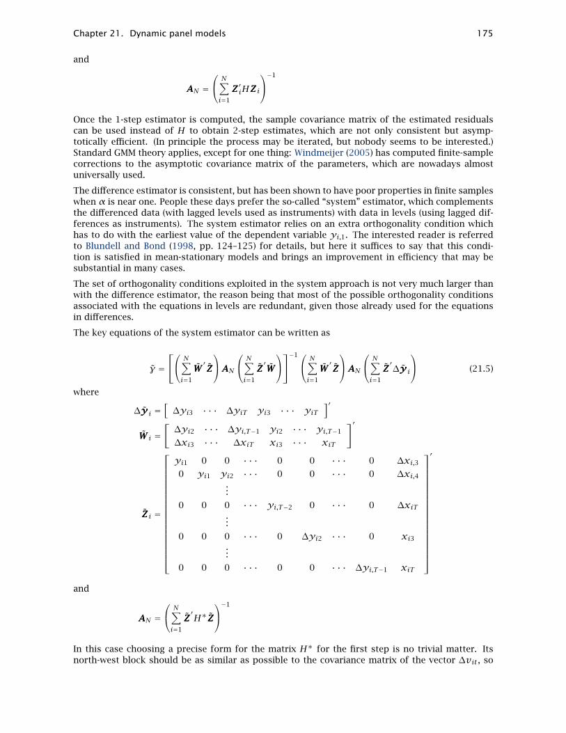
Chapter 21. Dynamic panel models 175
and
AAAN = N∑i=1
ZZZ′iHZZZi
−1
Once the 1-step estimator is computed, the sample covariance matrix of the estimated residualscan be used instead of H to obtain 2-step estimates, which are not only consistent but asymp-totically efficient. (In principle the process may be iterated, but nobody seems to be interested.)Standard GMM theory applies, except for one thing: Windmeijer (2005) has computed finite-samplecorrections to the asymptotic covariance matrix of the parameters, which are nowadays almostuniversally used.
The difference estimator is consistent, but has been shown to have poor properties in finite sampleswhen α is near one. People these days prefer the so-called “system” estimator, which complementsthe differenced data (with lagged levels used as instruments) with data in levels (using lagged dif-ferences as instruments). The system estimator relies on an extra orthogonality condition whichhas to do with the earliest value of the dependent variable yi,1. The interested reader is referredto Blundell and Bond (1998, pp. 124–125) for details, but here it suffices to say that this condi-tion is satisfied in mean-stationary models and brings an improvement in efficiency that may besubstantial in many cases.
The set of orthogonality conditions exploited in the system approach is not very much larger thanwith the difference estimator, the reason being that most of the possible orthogonality conditionsassociated with the equations in levels are redundant, given those already used for the equationsin differences.
The key equations of the system estimator can be written as
γ = N∑
i=1
WWW ′ZZZ
AAAN N∑i=1
ZZZ′WWW
−1 N∑i=1
WWW ′ZZZ
AAAN N∑i=1
ZZZ′∆yyyi (21.5)
where
∆yyyi = [ ∆yi3 · · · ∆yiT yi3 · · · yiT]′
WWW i =[ ∆yi2 · · · ∆yi,T−1 yi2 · · · yi,T−1∆xi3 · · · ∆xiT xi3 · · · xiT
]′
ZZZi =
yi1 0 0 · · · 0 0 · · · 0 ∆xi,30 yi1 yi2 · · · 0 0 · · · 0 ∆xi,4
...
0 0 0 · · · yi,T−2 0 · · · 0 ∆xiT...
0 0 0 · · · 0 ∆yi2 · · · 0 xi3...
0 0 0 · · · 0 0 · · · ∆yi,T−1 xiT
′
and
AAAN = N∑i=1
ZZZ′H∗ZZZ
−1
In this case choosing a precise form for the matrix H∗ for the first step is no trivial matter. Itsnorth-west block should be as similar as possible to the covariance matrix of the vector ∆vit , so

Chapter 21. Dynamic panel models 176
the same choice as the “difference” estimator is appropriate. Ideally, the south-east block shouldbe proportional to the covariance matrix of the vector ιιιηi + vvv , that is σ 2
v I + σ 2η ιιιιιι′; but since σ 2
η isunknown and any positive definite matrix renders the estimator consistent, people just use I. Theoff-diagonal blocks should, in principle, contain the covariances between ∆vis and vit , which wouldbe an identity matrix if vit is white noise. However, since the south-east block is typically given aconventional value anyway, the benefit in making this choice is not obvious. Some packages use I;others use a zero matrix. Asymptotically, it should not matter, but on real datasets the differencebetween the resulting estimates can be noticeable.
Rank deficiency
Both the difference estimator (21.4) and the system estimator (21.5) depend, for their existence,on the invertibility of AAAN . This matrix may turn out to be singular for several reasons. However,this does not mean that the estimator is not computable: in some cases, adjustments are possiblesuch that the estimator does exist, but the user should be aware that in these cases not all softwarepackages use the same strategy and replication of results may prove difficult or even impossible.
A first reason why AAAN may be singular could be the unavailability of instruments, chiefly becauseof missing observations. This case is easy to handle. If a particular row of ZZZi is zero for allunits, the corresponding orthogonality condition (or the corresponding instrument if you prefer) isautomatically dropped; of course, the overidentification rank is adjusted for testing purposes.
Even if no instruments are zero, however, AAAN could be rank deficient. A trivial case occurs if thereare collinear instruments, but a less trivial case may arise when T (the total number of time periodsavailable) is not much smaller thanN (the number of units), as, for example, in some macro datasetswhere the units are countries. The total number of potentially usable orthogonality conditions isO(T 2), which may well exceed N in some cases. Of course AAAN is the sum of N matrices which have,at most, rank 2T − 3 and therefore it could well happen that the sum is singular.
In all these cases, what we consider the “proper” way to go is to substitute the pseudo-inverse ofAAAN (Moore–Penrose) for its regular inverse. Again, our choice is shared by some software packages,but not all, so replication may be hard.
Treatment of missing values
Textbooks seldom bother with missing values, but in some cases their treatment may be far fromobvious. This is especially true if missing values are interspersed between valid observations. Forexample, consider the plain difference estimator with one lag, so
yt = αyt−1 + η+ εtwhere the i index is omitted for clarity. Suppose you have an individual with t = 1 . . .5, for whichy3 is missing. It may seem that the data for this individual are unusable, because differencing ytwould produce something like
t 1 2 3 4 5
yt ∗ ∗ ∗ ∗∆yt ∗ ∗where ∗ = nonmissing and = missing. Estimation seems to be unfeasible, since there are noperiods in which ∆yt and ∆yt−1 are both observable.
However, we can use a k-difference operator and get
∆kyt = α∆kyt−1 +∆kεtwhere ∆k = 1 − Lk and past levels of yt are perfectly valid instruments. In this example, we canchoose k = 3 and use y1 as an instrument, so this unit is in fact perfectly usable.
Not all software packages seem to be aware of this possibility, so replicating published results mayprove tricky if your dataset contains individuals with “gaps” between valid observations.

Chapter 21. Dynamic panel models 177
21.2 Usage
One of the concepts underlying the syntax of dpanel is that you get default values for severalchoices you may want to make, so that in a “standard” situation the command itself is very shortto write (and read). The simplest case of the model (21.1) is a plain AR(1) process:
yi,t = αyi,t−1 + ηi + vit . (21.6)
If you give the command
dpanel 1 ; y
gretl assumes that you want to estimate (21.6) via the difference estimator (21.4), using as manyorthogonality conditions as possible. The scalar 1 between dpanel and the semicolon indicates thatonly one lag of y is included as an explanatory variable; using 2 would give an AR(2) model. Thesyntax that gretl uses for the non-seasonal AR and MA lags in an ARMA model is also supported inthis context.1 For example, if you want the first and third lags of y (but not the second) included asexplanatory variables you can say
dpanel 1 3 ; y
or you can use a pre-defined matrix for this purpose:
matrix ylags = 1, 3dpanel ylags ; y
To use a single lag of y other than the first you need to employ this mechanism:
dpanel 3 ; y # only lag 3 is includeddpanel 3 ; y # compare: lags 1, 2 and 3 are used
To use the system estimator instead, you add the --system option, as in
dpanel 1 ; y --system
The level orthogonality conditions and the corresponding instrument are appended automatically(see eq. 21.5).
Regressors
If we want to introduce additional regressors, we list them after the dependent variable in the sameway as other gretl commands, such as ols.
For the difference orthogonality relations, dpanel takes care of transforming the regressors in par-allel with the dependent variable. Note that this differs from gretl’s arbond command, where onlythe dependent variable is differenced automatically; it brings us more in line with other software.
One case of potential ambiguity is when an intercept is specified but the difference-only estimatoris selected, as in
dpanel 1 ; y const
In this case the default dpanel behavior, which agrees with Stata’s xtabond2, is to drop the con-stant (since differencing reduces it to nothing but zeros). However, for compatibility with theDPD package for Ox, you can give the option --dpdstyle, in which case the constant is retained
1This represents an enhancement over the arbond command.

Chapter 21. Dynamic panel models 178
(equivalent to including a linear trend in equation 21.1). A similar point applies to the period-specific dummy variables which can be added in dpanel via the --time-dummies option: in thedifferences-only case these dummies are entered in differenced form by default, but when the--dpdstyle switch is applied they are entered in levels.
The standard gretl syntax applies if you want to use lagged explanatory variables, so for examplethe command
dpanel 1 ; y const x(0 to -1) --system
would result in estimation of the model
yit = αyi,t−1 + β0 + β1xit + β2xi,t−1 + ηi + vit .
Instruments
The default rules for instruments are:
• lags of the dependent variable are instrumented using all available orthogonality conditions;and
• additional regressors are considered exogenous, so they are used as their own instruments.
If a different policy is wanted, the instruments should be specified in an additional list, separatedfrom the regressors list by a semicolon. The syntax closely mirrors that for the tsls command,but in this context it is necessary to distinguish between “regular” instruments and what are oftencalled “GMM-style” instruments (that is, instruments that are handled in the same block-diagonalmanner as lags of the dependent variable, as described above).
“Regular” instruments are transformed in the same way as regressors, and the contemporaneousvalue of the transformed variable is used to form an orthogonality condition. Since regressors aretreated as exogenous by default, it follows that these two commands estimate the same model:
dpanel 1 ; y zdpanel 1 ; y z ; z
The instrument specification in the second case simply confirms what is implicit in the first: thatz is exogenous. Note, though, that if you have some additional variable z2 which you want to addas a regular instrument, it then becomes necessary to include z in the instrument list if it is to betreated as exogenous:
dpanel 1 ; y z ; z2 # z is now implicitly endogenousdpanel 1 ; y z ; z z2 # z is treated as exogenous
The specification of “GMM-style” instruments is handled by the special constructs GMM() andGMMlevel(). The first of these relates to instruments for the equations in differences, and thesecond to the equations in levels. The syntax for GMM() is
GMM(name, minlag, maxlag)
where name is replaced by the name of a series (or the name of a list of series), and minlag andmaxlag are replaced by the minimum and maximum lags to be used as instruments. The same goesfor GMMlevel().
One common use of GMM() is to limit the number of lagged levels of the dependent variable usedas instruments for the equations in differences. It’s well known that although exploiting all pos-sible orthogonality conditions yields maximal asymptotic efficiency, in finite samples it may bepreferable to use a smaller subset (but see also Okui (2009)). For example, the specification

Chapter 21. Dynamic panel models 179
dpanel 1 ; y ; GMM(y, 2, 4)
ensures that no lags of yt earlier than t − 4 will be used as instruments.
A second use of GMM() is to exploit more fully the potential block-diagonal orthogonality conditionsoffered by an exogenous regressor, or a related variable that does not appear as a regressor. Forexample, in
dpanel 1 ; y x ; GMM(z, 2, 6)
the variable x is considered an endogenous regressor, and up to 5 lags of z are used as instruments.
Note that in the following script fragment
dpanel 1 ; y zdpanel 1 ; y z ; GMM(z,0,0)
the two estimation commands should not be expected to give the same result, as the sets of orthog-onality relationships are subtly different. In the latter case, you have T − 2 separate orthogonalityrelationships pertaining to zit , none of which has any implication for the other ones; in the formercase, you only have one. In terms of the ZZZi matrix, the first form adds a single row to the bottomof the instruments matrix, while the second form adds a diagonal block with T − 2 columns; thatis, [
zi3 zi4 · · · zit]
versus zi3 0 · · · 0
0 zi4 · · · 0. . .
. . .
0 0 · · · zit
21.3 Replication of DPD results
In this section we show how to replicate the results of some of the pioneering work with dynamicpanel-data estimators by Arellano, Bond and Blundell. As the DPD manual (Doornik, Arellano andBond, 2006) explains, it is difficult to replicate the original published results exactly, for two mainreasons: not all of the data used in those studies are publicly available; and some of the choicesmade in the original software implementation of the estimators have been superseded. Here, there-fore, our focus is on replicating the results obtained using the current DPD package and reportedin the DPD manual.
The examples are based on the program files abest1.ox, abest3.ox and bbest1.ox. Theseare included in the DPD package, along with the Arellano–Bond database files abdata.bn7 andabdata.in7.2 The Arellano–Bond data are also provided with gretl, in the file abdata.gdt. In thefollowing we do not show the output from DPD or gretl; it is somewhat voluminous, and is easilygenerated by the user. As of this writing the results from Ox/DPD and gretl are identical in allrelevant respects for all of the examples shown.3
A complete Ox/DPD program to generate the results of interest takes this general form:
#include <oxstd.h>#import <packages/dpd/dpd>
2See http://www.doornik.com/download.html.3To be specific, this is using Ox Console version 5.10, version 1.24 of the DPD package, and gretl built from CVS as of
2010-10-23, all on Linux.

Chapter 21. Dynamic panel models 180
main()
decl dpd = new DPD();
dpd.Load("abdata.in7");dpd.SetYear("YEAR");
// model-specific code here
delete dpd;
In the examples below we take this template for granted and show just the model-specific code.
Example 1
The following Ox/DPD code—drawn from abest1.ox—replicates column (b) of Table 4 in Arellanoand Bond (1991), an instance of the differences-only or GMM-DIF estimator. The dependent variableis the log of employment, n; the regressors include two lags of the dependent variable, current andlagged values of the log real-product wage, w, the current value of the log of gross capital, k, andcurrent and lagged values of the log of industry output, ys. In addition the specification includesa constant and five year dummies; unlike the stochastic regressors, these deterministic terms arenot differenced. In this specification the regressors w, k and ys are treated as exogenous and serveas their own instruments. In DPD syntax this requires entering these variables twice, on the X_VARand I_VAR lines. The GMM-type (block-diagonal) instruments in this example are the second andsubsequent lags of the level of n. Both 1-step and 2-step estimates are computed.
dpd.SetOptions(FALSE); // don’t use robust standard errorsdpd.Select(Y_VAR, "n", 0, 2);dpd.Select(X_VAR, "w", 0, 1, "k", 0, 0, "ys", 0, 1);dpd.Select(I_VAR, "w", 0, 1, "k", 0, 0, "ys", 0, 1);
dpd.Gmm("n", 2, 99);dpd.SetDummies(D_CONSTANT + D_TIME);
print("\n\n***** Arellano & Bond (1991), Table 4 (b)");dpd.SetMethod(M_1STEP);dpd.Estimate();dpd.SetMethod(M_2STEP);dpd.Estimate();
Here is gretl code to do the same job:
open abdata.gdtlist X = w w(-1) k ys ys(-1)dpanel 2 ; n X const --time-dummies --asy --dpdstyledpanel 2 ; n X const --time-dummies --asy --two-step --dpdstyle
Note that in gretl the switch to suppress robust standard errors is --asymptotic, here abbreviatedto --asy.4 The --dpdstyle flag specifies that the constant and dummies should not be differenced,in the context of a GMM-DIF model. With gretl’s dpanel command it is not necessary to specify theexogenous regressors as their own instruments since this is the default; similarly, the use of thesecond and all longer lags of the dependent variable as GMM-type instruments is the default andneed not be stated explicitly.
4Option flags in gretl can always be truncated, down to the minimal unique abbreviation.

Chapter 21. Dynamic panel models 181
Example 2
The DPD file abest3.ox contains a variant of the above that differs with regard to the choice ofinstruments: the variables w and k are now treated as predetermined, and are instrumented GMM-style using the second and third lags of their levels. This approximates column (c) of Table 4 inArellano and Bond (1991). We have modified the code in abest3.ox slightly to allow the use ofrobust (Windmeijer-corrected) standard errors, which are the default in both DPD and gretl with2-step estimation:
dpd.Select(Y_VAR, "n", 0, 2);dpd.Select(X_VAR, "w", 0, 1, "k", 0, 0, "ys", 0, 1);dpd.Select(I_VAR, "ys", 0, 1);dpd.SetDummies(D_CONSTANT + D_TIME);
dpd.Gmm("n", 2, 99);dpd.Gmm("w", 2, 3);dpd.Gmm("k", 2, 3);
print("\n***** Arellano & Bond (1991), Table 4 (c)\n");print(" (but using different instruments!!)\n");dpd.SetMethod(M_2STEP);dpd.Estimate();
The gretl code is as follows:
open abdata.gdtlist X = w w(-1) k ys ys(-1)list Ivars = ys ys(-1)dpanel 2 ; n X const ; GMM(w,2,3) GMM(k,2,3) Ivars --time --two-step --dpd
Note that since we are now calling for an instrument set other then the default (following the secondsemicolon), it is necessary to include the Ivars specification for the variable ys. However, it isnot necessary to specify GMM(n,2,99) since this remains the default treatment of the dependentvariable.
Example 3
Our third example replicates the DPD output from bbest1.ox: this uses the same dataset as theprevious examples but the model specifications are based on Blundell and Bond (1998), and involvecomparison of the GMM-DIF and GMM-SYS (“system”) estimators. The basic specification is slightlysimplified in that the variable ys is not used and only one lag of the dependent variable appears asa regressor. The Ox/DPD code is:
dpd.Select(Y_VAR, "n", 0, 1);dpd.Select(X_VAR, "w", 0, 1, "k", 0, 1);dpd.SetDummies(D_CONSTANT + D_TIME);
print("\n\n***** Blundell & Bond (1998), Table 4: 1976-86 GMM-DIF");dpd.Gmm("n", 2, 99);dpd.Gmm("w", 2, 99);dpd.Gmm("k", 2, 99);dpd.SetMethod(M_2STEP);dpd.Estimate();
print("\n\n***** Blundell & Bond (1998), Table 4: 1976-86 GMM-SYS");dpd.GmmLevel("n", 1, 1);dpd.GmmLevel("w", 1, 1);

Chapter 21. Dynamic panel models 182
dpd.GmmLevel("k", 1, 1);dpd.SetMethod(M_2STEP);dpd.Estimate();
Here is the corresponding gretl code:
open abdata.gdtlist X = w w(-1) k k(-1)list Z = w k
# Blundell & Bond (1998), Table 4: 1976-86 GMM-DIFdpanel 1 ; n X const ; GMM(Z,2,99) --time --two-step --dpd
# Blundell & Bond (1998), Table 4: 1976-86 GMM-SYSdpanel 1 ; n X const ; GMM(Z,2,99) GMMlevel(Z,1,1) \--time --two-step --dpd --system
Note the use of the --system option flag to specify GMM-SYS, including the default treatment ofthe dependent variable, which corresponds to GMMlevel(n,1,1). In this case we also want touse lagged differences of the regressors w and k as instruments for the levels equations so weneed explicit GMMlevel entries for those variables. If you want something other than the defaulttreatment for the dependent variable as an instrument for the levels equations, you should give anexplicit GMMlevel specification for that variable—and in that case the --system flag is redundant(but harmless).
For the sake of completeness, note that if you specify at least one GMMlevel term, dpanel will theninclude equations in levels, but it will not automatically add a default GMMlevel specification forthe dependent variable unless the --system option is given.
21.4 Cross-country growth example
The previous examples all used the Arellano–Bond dataset; for this example we use the datasetCEL.gdt, which is also included in the gretl distribution. As with the Arellano–Bond data, thereare numerous missing values. Details of the provenance of the data can be found by opening thedataset information window in the gretl GUI (Data menu, Dataset info item). This is a subset of theBarro–Lee 138-country panel dataset, an approximation to which is used in Caselli, Esquivel andLefort (1996) and Bond, Hoeffler and Temple (2001).5 Both of these papers explore the dynamicpanel-data approach in relation to the issues of growth and convergence of per capita income acrosscountries.
The dependent variable is growth in real GDP per capita over successive five-year periods; theregressors are the log of the initial (five years prior) value of GDP per capita, the log-ratio of in-vestment to GDP, s, in the prior five years, and the log of annual average population growth, n,over the prior five years plus 0.05 as stand-in for the rate of technical progress, g, plus the rate ofdepreciation, δ (with the last two terms assumed to be constant across both countries and periods).The original model is
∆5yit = βyi,t−5 +αsit + γ(nit + g + δ)+ νt + ηi + εit (21.7)
which allows for a time-specific disturbance νt . The Solow model with Cobb–Douglas productionfunction implies that γ = −α, but this assumption is not imposed in estimation. The time-specificdisturbance is eliminated by subtracting the period mean from each of the series.
5We say an “approximation” because we have not been able to replicate exactly the OLS results reported in the paperscited, though it seems from the description of the data in Caselli et al. (1996) that we ought to be able to do so. We notethat Bond et al. (2001) used data provided by Professor Caselli yet did not manage to reproduce the latter’s results.

Chapter 21. Dynamic panel models 183
Equation (21.7) can be transformed to an AR(1) dynamic panel-data model by adding yi,t−5 to bothsides, which gives
yit = (1+ β)yi,t−5 +αsit + γ(nit + g + δ)+ ηi + εit (21.8)
where all variables are now assumed to be time-demeaned.
In (rough) replication of Bond et al. (2001) we now proceed to estimate the following two models:(a) equation (21.8) via GMM-DIF, using as instruments the second and all longer lags of yit , sit andnit + g + δ; and (b) equation (21.8) via GMM-SYS, using ∆yi,t−1, ∆si,t−1 and ∆(ni,t−1 + g + δ) asadditional instruments in the levels equations. We report robust standard errors throughout. (As apurely notational matter, we now use “t−1” to refer to values five years prior to t, as in Bond et al.(2001)).
The gretl script to do this job is shown below. Note that the final transformed versions of thevariables (logs, with time-means subtracted) are named ly (yit), linv (sit) and lngd (nit + g + δ).
open CEL.gdt
ngd = n + 0.05ly = log(y)linv = log(s)lngd = log(ngd)
# take out time meansloop i=1..8 --quietsmpl (time == i) --restrict --replacely -= mean(ly)linv -= mean(linv)lngd -= mean(lngd)
endloop
smpl --fulllist X = linv lngd# 1-step GMM-DIFdpanel 1 ; ly X ; GMM(X,2,99)# 2-step GMM-DIFdpanel 1 ; ly X ; GMM(X,2,99) --two-step# GMM-SYSdpanel 1 ; ly X ; GMM(X,2,99) GMMlevel(X,1,1) --two-step --sys
For comparison we estimated the same two models using Ox/DPD and the Stata command xtabond2.(In each case we constructed a comma-separated values dataset containing the data as transformedin the gretl script shown above, using a missing-value code appropriate to the target program.) Forreference, the commands used with Stata are reproduced below:
insheet using CEL.csvtsset unit timextabond2 ly L.ly linv lngd, gmm(L.ly, lag(1 99)) gmm(linv, lag(2 99))gmm(lngd, lag(2 99)) rob nolev
xtabond2 ly L.ly linv lngd, gmm(L.ly, lag(1 99)) gmm(linv, lag(2 99))gmm(lngd, lag(2 99)) rob nolev twostep
xtabond2 ly L.ly linv lngd, gmm(L.ly, lag(1 99)) gmm(linv, lag(2 99))gmm(lngd, lag(2 99)) rob nocons twostep
For the GMM-DIF model all three programs find 382 usable observations and 30 instruments, andyield identical parameter estimates and robust standard errors (up to the number of digits printed,or more); see Table 21.1.6
6The coefficient shown for ly(-1) in the Tables is that reported directly by the software; for comparability with theoriginal model (eq. 21.7) it is necesary to subtract 1, which produces the expected negative value indicating conditionalconvergence in per capita income.

Chapter 21. Dynamic panel models 184
1-step 2-step
coeff std. error coeff std. error
ly(-1) 0.577564 0.1292 0.610056 0.1562
linv 0.0565469 0.07082 0.100952 0.07772
lngd −0.143950 0.2753 −0.310041 0.2980
Table 21.1: GMM-DIF: Barro–Lee data
Results for GMM-SYS estimation are shown in Table 21.2. In this case we show two sets of gretlresults: those labeled “gretl(1)” were obtained using gretl’s --dpdstyle option, while those labeled“gretl(2)” did not use that option—the intent being to reproduce the H matrices used by Ox/DPDand xtabond2 respectively.
gretl(1) Ox/DPD gretl(2) xtabond2
ly(-1) 0.9237 (0.0385) 0.9167 (0.0373) 0.9073 (0.0370) 0.9073 (0.0370)
linv 0.1592 (0.0449) 0.1636 (0.0441) 0.1856 (0.0411) 0.1856 (0.0411)
lngd −0.2370 (0.1485) −0.2178 (0.1433) −0.2355 (0.1501) −0.2355 (0.1501)
Table 21.2: 2-step GMM-SYS: Barro–Lee data (standard errors in parentheses)
In this case all three programs use 479 observations; gretl and xtabond2 use 41 instruments andproduce the same estimates (when using the same H matrix) while Ox/DPD nominally uses 66.7
It is noteworthy that with GMM-SYS plus “messy” missing observations, the results depend on theprecise array of instruments used, which in turn depends on the details of the implementation ofthe estimator.
21.5 Auxiliary test statistics
We have concentrated above on the parameter estimates and standard errors. It may be worthadding a few words on the additional test statistics that typically accompany both GMM-DIF andGMM-SYS estimation. These include the Sargan test for overidentification, one or more Wald testsfor the joint significance of the regressors (and time dummies, if applicable) and tests for first- andsecond-order autocorrelation of the residuals from the equations in differences.
As in Ox/DPD, the Sargan test statistic reported by gretl is
S = N∑i=1
vvv∗′i ZZZi
AAAN N∑i=1
ZZZ′ivvv∗i
where the vvv∗i are the transformed (e.g. differenced) residuals for unit i. Under the null hypothesisthat the instruments are valid, S is asymptotically distributed as chi-square with degrees of freedomequal to the number of overidentifying restrictions.
In general we see a good level of agreement between gretl, DPD and xtabond2 with regard to thesestatistics, with a few relatively minor exceptions. Specifically, xtabond2 computes both a “Sargantest” and a “Hansen test” for overidentification, but what it calls the Hansen test is, apparently, whatDPD calls the Sargan test. (We have had difficulty determining from the xtabond2 documentation(Roodman, 2006) exactly how its Sargan test is computed.) In addition there are cases where thedegrees of freedom for the Sargan test differ between DPD and gretl; this occurs when the AAANmatrix is singular (section 21.1). In concept the df equals the number of instruments minus the
7This is a case of the issue described in section 21.1: the full AAAN matrix turns out to be singular and special measuresmust be taken to produce estimates.

Chapter 21. Dynamic panel models 185
number of parameters estimated; for the first of these terms gretl uses the rank of AAAN , while DPDappears to use the full dimension of this matrix.
21.6 Memo: dpanel options
flag effect
--asymptotic Suppresses the use of robust standard errors
--two-step Calls for 2-step estimation (the default being 1-step)
--system Calls for GMM-SYS, with default treatment of the dependent variable,as in GMMlevel(y,1,1)
--time-dummies Includes period-specific dummy variables
--dpdstyle Compute the H matrix as in DPD; also suppresses differencing ofautomatic time dummies and omission of intercept in the GMM-DIFcase
--verbose When --two-step is selected, prints the 1-step estimates first
--vcv Calls for printing of the covariance matrix
--quiet Suppresses the printing of results
The time dummies option supports the qualifier noprint, as in
--time-dummies=noprint
This means that although the dummies are included in the specification their coefficients, standarderrors and so on are not printed.

Chapter 22
Nonlinear least squares
22.1 Introduction and examples
Gretl supports nonlinear least squares (NLS) using a variant of the Levenberg–Marquardt algorithm.The user must supply a specification of the regression function; prior to giving this specification theparameters to be estimated must be “declared” and given initial values. Optionally, the user maysupply analytical derivatives of the regression function with respect to each of the parameters.If derivatives are not given, the user must instead give a list of the parameters to be estimated(separated by spaces or commas), preceded by the keyword params. The tolerance (criterion forterminating the iterative estimation procedure) can be adjusted using the set command.
The syntax for specifying the function to be estimated is the same as for the genr command. Hereare two examples, with accompanying derivatives.
# Consumption function from Greenenls C = alpha + beta * Y^gamma
deriv alpha = 1deriv beta = Y^gammaderiv gamma = beta * Y^gamma * log(Y)
end nls
# Nonlinear function from Russell Davidsonnls y = alpha + beta * x1 + (1/beta) * x2
deriv alpha = 1deriv beta = x1 - x2/(beta*beta)
end nls --vcv
Note the command words nls (which introduces the regression function), deriv (which introducesthe specification of a derivative), and end nls, which terminates the specification and calls forestimation. If the --vcv flag is appended to the last line the covariance matrix of the parameterestimates is printed.
22.2 Initializing the parameters
The parameters of the regression function must be given initial values prior to the nls command.This can be done using the genr command (or, in the GUI program, via the menu item “Variable,Define new variable”).
In some cases, where the nonlinear function is a generalization of (or a restricted form of) a linearmodel, it may be convenient to run an ols and initialize the parameters from the OLS coefficientestimates. In relation to the first example above, one might do:
ols C 0 Ygenr alpha = $coeff(0)genr beta = $coeff(Y)genr gamma = 1
And in relation to the second example one might do:
186

Chapter 22. Nonlinear least squares 187
ols y 0 x1 x2genr alpha = $coeff(0)genr beta = $coeff(x1)
22.3 NLS dialog window
It is probably most convenient to compose the commands for NLS estimation in the form of agretl script but you can also do so interactively, by selecting the item “Nonlinear Least Squares”under the “Model, Nonlinear models” menu. This opens a dialog box where you can type thefunction specification (possibly prefaced by genr lines to set the initial parameter values) and thederivatives, if available. An example of this is shown in Figure 22.1. Note that in this context youdo not have to supply the nls and end nls tags.
Figure 22.1: NLS dialog box
22.4 Analytical and numerical derivatives
If you are able to figure out the derivatives of the regression function with respect to the param-eters, it is advisable to supply those derivatives as shown in the examples above. If that is notpossible, gretl will compute approximate numerical derivatives. However, the properties of the NLSalgorithm may not be so good in this case (see section 22.8).
This is done by using the params statement, which should be followed by a list of identifierscontaining the parameters to be estimated. In this case, the examples above would read as follows:
# Greenenls C = alpha + beta * Y^gamma
params alpha beta gammaend nls
# Davidsonnls y = alpha + beta * x1 + (1/beta) * x2
params alpha betaend nls
If analytical derivatives are supplied, they are checked for consistency with the given nonlinearfunction. If the derivatives are clearly incorrect estimation is aborted with an error message. If the

Chapter 22. Nonlinear least squares 188
derivatives are “suspicious” a warning message is issued but estimation proceeds. This warningmay sometimes be triggered by incorrect derivatives, but it may also be triggered by a high degreeof collinearity among the derivatives.
Note that you cannot mix analytical and numerical derivatives: you should supply expressions forall of the derivatives or none.
22.5 Advanced use
The nls block can also contain more sophisticated constructs. First, it can handle intermediateexpressions; this makes it possible to construct the conditional mean expression as a multi-stepjob, thus enhancing modularity and readability of the code. Second, more complex objects, such aslists and matrices, can be used for this purpose.
For example, suppose that we want to estimate a Probit Binary Response model via NLS. The speci-fication is
yi = Φ [g(xxxi)]+ui, g(xxxi) = b0 + b1x1,i + b2x2,i = bbb′xxxi (22.1)
Note: this is not the recommended way to estimate a probit model: the ui term is heteroskedasticby construction and ML estimation is much preferable here. Still, NLS is a consistent estimator ofthe parameter vector bbb, although its covariance matrix will have to be adjusted to compensate forheteroskedasticity: this is accomplished via the --robust switch.
Listing 22.1: NLS estimation of a Probit model
open greene25_1.gdtlist X = const age income ownrent selfempl
# initalisationols cardhldr X --quietmatrix b = $coeff / $sigma
# proceed with NLS estimationnls cardhldr = cnorm(ndx)
series ndx = lincomb(X, b)params b
end nls --robust
# compare with ML probitprobit cardhldr X --p-values
The example in script 22.1 can be enhanced by using analytical derivatives: since
∂g(xxxi)∂bj
=ϕ(bbb′xxxi) · xij
one could substitute the params line in the script with the two-liner
series f = dnorm(ndx)deriv b = f .* X
and have nls use analytically-computed derivatives, which are quicker and usually more reliable.

Chapter 22. Nonlinear least squares 189
22.6 Controlling termination
The NLS estimation procedure is an iterative process. Iteration is terminated when the criterion forconvergence is met or when the maximum number of iterations is reached, whichever comes first.
Let k denote the number of parameters being estimated. The maximum number of iterations is100 × (k + 1) when analytical derivatives are given, and 200 × (k + 1) when numerical derivativesare used.
Let ε denote a small number. The iteration is deemed to have converged if at least one of thefollowing conditions is satisfied:
• Both the actual and predicted relative reductions in the error sum of squares are at most ε.
• The relative error between two consecutive iterates is at most ε.
This default value of ε is the machine precision to the power 3/4,1 but it can be adjusted using theset command with the parameter nls_toler. For example
set nls_toler .0001
will relax the value of ε to 0.0001.
22.7 Details on the code
The underlying engine for NLS estimation is based on the minpack suite of functions, availablefrom netlib.org. Specifically, the following minpack functions are called:
lmder Levenberg–Marquardt algorithm with analytical derivatives
chkder Check the supplied analytical derivatives
lmdif Levenberg–Marquardt algorithm with numerical derivatives
fdjac2 Compute final approximate Jacobian when using numerical derivatives
dpmpar Determine the machine precision
On successful completion of the Levenberg–Marquardt iteration, a Gauss–Newton regression is usedto calculate the covariance matrix for the parameter estimates. If the --robust flag is given arobust variant is computed. The documentation for the set command explains the specific optionsavailable in this regard.
Since NLS results are asymptotic, there is room for debate over whether or not a correction fordegrees of freedom should be applied when calculating the standard error of the regression (andthe standard errors of the parameter estimates). For comparability with OLS, and in light of thereasoning given in Davidson and MacKinnon (1993), the estimates shown in gretl do use a degreesof freedom correction.
22.8 Numerical accuracy
Table 22.1 shows the results of running the gretl NLS procedure on the 27 Statistical ReferenceDatasets made available by the U.S. National Institute of Standards and Technology (NIST) for test-ing nonlinear regression software.2 For each dataset, two sets of starting values for the parametersare given in the test files, so the full test comprises 54 runs. Two full tests were performed, one
1On a 32-bit Intel Pentium machine a likely value for this parameter is 1.82× 10−12.2For a discussion of gretl’s accuracy in the estimation of linear models, see Appendix D.

Chapter 22. Nonlinear least squares 190
using all analytical derivatives and one using all numerical approximations. In each case the defaulttolerance was used.3
Out of the 54 runs, gretl failed to produce a solution in 4 cases when using analytical derivatives,and in 5 cases when using numeric approximation. Of the four failures in analytical derivativesmode, two were due to non-convergence of the Levenberg–Marquardt algorithm after the maximumnumber of iterations (on MGH09 and Bennett5, both described by NIST as of “Higher difficulty”) andtwo were due to generation of range errors (out-of-bounds floating point values) when computingthe Jacobian (on BoxBOD and MGH17, described as of “Higher difficulty” and “Average difficulty”respectively). The additional failure in numerical approximation mode was on MGH10 (“Higher diffi-culty”, maximum number of iterations reached).
The table gives information on several aspects of the tests: the number of outright failures, theaverage number of iterations taken to produce a solution and two sorts of measure of the accuracyof the estimates for both the parameters and the standard errors of the parameters.
For each of the 54 runs in each mode, if the run produced a solution the parameter estimatesobtained by gretl were compared with the NIST certified values. We define the “minimum correctfigures” for a given run as the number of significant figures to which the least accurate gretl esti-mate agreed with the certified value, for that run. The table shows both the average and the worstcase value of this variable across all the runs that produced a solution. The same information isshown for the estimated standard errors.4
The second measure of accuracy shown is the percentage of cases, taking into account all parame-ters from all successful runs, in which the gretl estimate agreed with the certified value to at leastthe 6 significant figures which are printed by default in the gretl regression output.
Table 22.1: Nonlinear regression: the NIST tests
Analytical derivatives Numerical derivatives
Failures in 54 tests 4 5
Average iterations 32 127
Mean of min. correct figures, 8.120 6.980
parameters
Worst of min. correct figures, 4 3
parameters
Mean of min. correct figures, 8.000 5.673
standard errors
Worst of min. correct figures, 5 2
standard errors
Percent correct to at least 6 figures, 96.5 91.9
parameters
Percent correct to at least 6 figures, 97.7 77.3
standard errors
Using analytical derivatives, the worst case values for both parameters and standard errors wereimproved to 6 correct figures on the test machine when the tolerance was tightened to 1.0e−14.
3The data shown in the table were gathered from a pre-release build of gretl version 1.0.9, compiled with gcc 3.3,linked against glibc 2.3.2, and run under Linux on an i686 PC (IBM ThinkPad A21m).
4For the standard errors, I excluded one outlier from the statistics shown in the table, namely Lanczos1. This is anodd case, using generated data with an almost-exact fit: the standard errors are 9 or 10 orders of magnitude smallerthan the coefficients. In this instance gretl could reproduce the certified standard errors to only 3 figures (analyticalderivatives) and 2 figures (numerical derivatives).

Chapter 22. Nonlinear least squares 191
Using numerical derivatives, the same tightening of the tolerance raised the worst values to 5correct figures for the parameters and 3 figures for standard errors, at a cost of one additionalfailure of convergence.
Note the overall superiority of analytical derivatives: on average solutions to the test problemswere obtained with substantially fewer iterations and the results were more accurate (most notablyfor the estimated standard errors). Note also that the six-digit results printed by gretl are not 100percent reliable for difficult nonlinear problems (in particular when using numerical derivatives).Having registered this caveat, the percentage of cases where the results were good to six digits orbetter seems high enough to justify their printing in this form.

Chapter 23
Maximum likelihood estimation
23.1 Generic ML estimation with gretl
Maximum likelihood estimation is a cornerstone of modern inferential procedures. Gretl providesa way to implement this method for a wide range of estimation problems, by use of the mle com-mand. We give here a few examples.
To give a foundation for the examples that follow, we start from a brief reminder on the basicsof ML estimation. Given a sample of size T , it is possible to define the density function1 for thewhole sample, namely the joint distribution of all the observations f(Y;θ), where Y =
y1, . . . , yT
.
Its shape is determined by a k-vector of unknown parameters θ, which we assume is contained ina set Θ, and which can be used to evaluate the probability of observing a sample with any givencharacteristics.
After observing the data, the values Y are given, and this function can be evaluated for any legiti-mate value of θ. In this case, we prefer to call it the likelihood function; the need for another namestems from the fact that this function works as a density when we use the yts as arguments and θas parameters, whereas in this context θ is taken as the function’s argument, and the data Y onlyhave the role of determining its shape.
In standard cases, this function has a unique maximum. The location of the maximum is unaffectedif we consider the logarithm of the likelihood (or log-likelihood for short): this function will bedenoted as
`(θ) = logf(Y;θ)
The log-likelihood functions that gretl can handle are those where `(θ) can be written as
`(θ) =T∑t=1
`t(θ)
which is true in most cases of interest. The functions `t(θ) are called the log-likelihood contribu-tions.
Moreover, the location of the maximum is obviously determined by the data Y. This means that thevalue
θ(Y) = Argmaxθ∈Θ `(θ) (23.1)
is some function of the observed data (a statistic), which has the property, under mild conditions,of being a consistent, asymptotically normal and asymptotically efficient estimator of θ.
Sometimes it is possible to write down explicitly the function θ(Y); in general, it need not be so. Inthese circumstances, the maximum can be found by means of numerical techniques. These oftenrely on the fact that the log-likelihood is a smooth function of θ, and therefore on the maximumits partial derivatives should all be 0. The gradient vector, or score vector, is a function that enjoysmany interesting statistical properties in its own right; it will be denoted here as g(θ). It is a
1We are supposing here that our data are a realization of continuous random variables. For discrete random variables,everything continues to apply by referring to the probability function instead of the density. In both cases, the distributionmay be conditional on some exogenous variables.
192

Chapter 23. Maximum likelihood estimation 193
k-vector with typical element
gi(θ) =∂`(θ)∂θi
=T∑t=1
∂`t(θ)∂θi
Gradient-based methods can be shortly illustrated as follows:
1. pick a point θ0 ∈ Θ;
2. evaluate g(θ0);
3. if g(θ0) is “small”, stop. Otherwise, compute a direction vector d(g(θ0));
4. evaluate θ1 = θ0 + d(g(θ0));
5. substitute θ0 with θ1;
6. restart from 2.
Many algorithms of this kind exist; they basically differ from one another in the way they computethe direction vector d(g(θ0)), to ensure that `(θ1) > `(θ0) (so that we eventually end up on themaximum).
The default method gretl uses to maximize the log-likelihood is a gradient-based algorithm knownas the BFGS (Broyden, Fletcher, Goldfarb and Shanno) method. This technique is used in mosteconometric and statistical packages, as it is well-established and remarkably powerful. Clearly,in order to make this technique operational, it must be possible to compute the vector g(θ) forany value of θ. In some cases this vector can be written explicitly as a function of Y. If this isnot possible or too difficult the gradient may be evaluated numerically. The alternative Newton-Raphson algorithm is also available, which is more effective under some circumstances but is alsomore fragile; see section 23.8 and chapter 34 for details.
The choice of the starting value, θ0, is crucial in some contexts and inconsequential in others. Ingeneral, however, it is advisable to start the algorithm from “sensible” values whenever possible. Ifa consistent estimator is available, this is usually a safe and efficient choice: this ensures that inlarge samples the starting point will be likely close to θ and convergence can be achieved in fewiterations.
The maximum number of iterations allowed for the BFGS procedure, and the relative tolerancefor assessing convergence, can be adjusted using the set command: the relevant variables arebfgs_maxiter (default value 500) and bfgs_toler (default value, the machine precision to thepower 3/4).
Covariance matrix and standard errors
By default the covariance matrix of the parameter estimates is based on the Outer Product of theGradient. That is,
VarOPG(θ) =(G′(θ)G(θ)
)−1(23.2)
where G(θ) is the T × k matrix of contributions to the gradient. Two other options are available. Ifthe --hessian flag is given, the covariance matrix is computed from a numerical approximation tothe Hessian at convergence. If the --robust option is selected, the quasi-ML “sandwich” estimatoris used:
VarQML(θ) = H(θ)−1G′(θ)G(θ)H(θ)−1
where H denotes the numerical approximation to the Hessian.
Chapter 23. Maximum likelihood estimation 194
23.2 Gamma estimation
Suppose we have a sample of T independent and identically distributed observations from a Gammadistribution. The density function for each observation xt is
f(xt) =αpΓ(p)xp−1
t exp (−αxt) (23.3)
The log-likelihood for the entire sample can be written as the logarithm of the joint density of allthe observations. Since these are independent and identical, the joint density is the product of theindividual densities, and hence its log is
`(α,p) =T∑t=1
log
[αpΓ(p)xp−1
t exp (−αxt)]=
T∑t=1
`t (23.4)
where`t = p · log(αxt)− γ(p)− logxt −αxt
and γ(·) is the log of the gamma function. In order to estimate the parameters α and p via ML, weneed to maximize (23.4) with respect to them. The corresponding gretl code snippet is
scalar alpha = 1scalar p = 1
mle logl = p*ln(alpha * x) - lngamma(p) - ln(x) - alpha * xparams alpha p
end mle
The first two statements
alpha = 1p = 1
are necessary to ensure that the variables alpha and p exist before the computation of logl isattempted. Inside the mle block these variables (which could be either scalars, vectors or a com-bination of the two — see below for an example) are identified as the parameters that should beadjusted to maximize the likelihood via the params keyword. Their values will be changed by theexecution of the mle command; upon successful completion, they will be replaced by the ML esti-mates. The starting value is 1 for both; this is arbitrary and does not matter much in this example(more on this later).
The above code can be made more readable, and marginally more efficient, by defining a variableto hold α · xt . This command can be embedded in the mle block as follows:
mle logl = p*ln(ax) - lngamma(p) - ln(x) - axseries ax = alpha*xparams alpha p
end mle
The variable ax is not added to the params list, of course, since it is just an auxiliary variable tofacilitate the calculations. You can insert as many such auxiliary lines as you require before theparams line, with the restriction that they must contain either (a) commands to generate series,scalars or matrices or (b) print commands (which may be used to aid in debugging).
In a simple example like this, the choice of the starting values is almost inconsequential; the algo-rithm is likely to converge no matter what the starting values are. However, consistent method-of-moments estimators of p and α can be simply recovered from the sample meanm and variance V :since it can be shown that
E(xt) = p/α V(xt) = p/α2

Chapter 23. Maximum likelihood estimation 195
it follows that the following estimators
α = m/Vp = m · α
are consistent, and therefore suitable to be used as starting point for the algorithm. The gretl scriptcode then becomes
scalar m = mean(x)scalar alpha = m/var(x)scalar p = m*alpha
mle logl = p*ln(ax) - lngamma(p) - ln(x) - axseries ax = alpha*xparams alpha p
end mle
Another thing to note is that sometimes parameters are constrained within certain boundaries: inthis case, for example, both α and p must be positive numbers. Gretl does not check for this: itis the user’s responsibility to ensure that the function is always evaluated at an admissible pointin the parameter space during the iterative search for the maximum. An effective technique is todefine a variable for checking that the parameters are admissible and setting the log-likelihood asundefined if the check fails. An example, which uses the conditional assignment operator, follows:
scalar m = mean(x)scalar alpha = m/var(x)scalar p = m*alpha
mle logl = check ? p*ln(ax) - lngamma(p) - ln(x) - ax : NAseries ax = alpha*xscalar check = (alpha>0) && (p>0)params alpha p
end mle
23.3 Stochastic frontier cost function
When modeling a cost function, it is sometimes worthwhile to incorporate explicitly into the sta-tistical model the notion that firms may be inefficient, so that the observed cost deviates from thetheoretical figure not only because of unobserved heterogeneity between firms, but also becausetwo firms could be operating at a different efficiency level, despite being identical under all otherrespects. In this case we may write
Ci = C∗i +ui + viwhere Ci is some variable cost indicator, C∗i is its “theoretical” value, ui is a zero-mean disturbanceterm and vi is the inefficiency term, which is supposed to be nonnegative by its very nature.
A linear specification for C∗i is often chosen. For example, the Cobb–Douglas cost function ariseswhen C∗i is a linear function of the logarithms of the input prices and the output quantities.
The stochastic frontier model is a linear model of the form yi = xiβ + εi in which the error termεi is the sum of ui and vi. A common postulate is that ui ∼ N(0, σ 2
u) and vi ∼∣∣N(0, σ 2
v)∣∣. If
independence between ui and vi is also assumed, then it is possible to show that the densityfunction of εi has the form:
f(εi) =√
2πΦ(λεi
σ
)1σφ(εiσ
)(23.5)
where Φ(·) andφ(·) are, respectively, the distribution and density function of the standard normal,
σ =√σ 2u + σ 2
v and λ = σuσv .

Chapter 23. Maximum likelihood estimation 196
As a consequence, the log-likelihood for one observation takes the form (apart form an irrelevantconstant)
`t = logΦ(λεiσ
)−[
log(σ)+ε2i
2σ 2
]Therefore, a Cobb–Douglas cost function with stochastic frontier is the model described by thefollowing equations:
logCi = logC∗i + εi
logC∗i = c +m∑j=1
βj logyij +n∑j=1
αj logpij
εi = ui + viui ∼ N(0, σ 2
u)
vi ∼∣∣∣N(0, σ 2
v)∣∣∣
In most cases, one wants to ensure that the homogeneity of the cost function with respect tothe prices holds by construction. Since this requirement is equivalent to
∑nj=1αj = 1, the above
equation for C∗i can be rewritten as
logCi − logpin = c +m∑j=1
βj logyij +n∑j=2
αj(logpij − logpin)+ εi (23.6)
The above equation could be estimated by OLS, but it would suffer from two drawbacks: first,the OLS estimator for the intercept c is inconsistent because the disturbance term has a non-zeroexpected value; second, the OLS estimators for the other parameters are consistent, but inefficientin view of the non-normality of εi. Both issues can be addressed by estimating (23.6) by maximumlikelihood. Nevertheless, OLS estimation is a quick and convenient way to provide starting valuesfor the MLE algorithm.
Listing 23.1 shows how to implement the model described so far. The banks91 file contains partof the data used in Lucchetti, Papi and Zazzaro (2001).
The script in example 23.1 is relatively easy to modify to show how one can use vectors (that is,1-dimensional matrices) for storing the parameters to optimize: example 23.2 holds essentially thesame script in which the parameters of the cost function are stored together in a vector. Of course,this makes also possible to use variable lists and other refinements which make the code morecompact and readable.
23.4 GARCH models
GARCH models are handled by gretl via a native function. However, it is instructive to see how theycan be estimated through the mle command.2
The following equations provide the simplest example of a GARCH(1,1) model:
yt = µ + εtεt = ut · σtut ∼ N(0,1)ht = ω+αε2
t−1 + βht−1.
Since the variance of yt depends on past values, writing down the log-likelihood function is notsimply a matter of summing the log densities for individual observations. As is common in time
2The gig addon, which handles other variants of conditionally heteroskedastic models, uses mle as its internal engine.

Chapter 23. Maximum likelihood estimation 197
Listing 23.1: Estimation of stochastic frontier cost function (with scalar parameters)
open banks91.gdt
# transformationsseries cost = ln(VC)series q1 = ln(Q1)series q2 = ln(Q2)series p1 = ln(P1)series p2 = ln(P2)series p3 = ln(P3)
# Cobb-Douglas cost function with homogeneity restrictions# (for initialization)genr rcost = cost - p1genr rp2 = p2 - p1genr rp3 = p3 - p1
ols rcost const q1 q2 rp2 rp3
# Cobb-Douglas cost function with homogeneity restrictions# and inefficiency
scalar b0 = $coeff(const)scalar b1 = $coeff(q1)scalar b2 = $coeff(q2)scalar b3 = $coeff(rp2)scalar b4 = $coeff(rp3)
scalar su = 0.1scalar sv = 0.1
mle logl = ln(cnorm(e*lambda/ss)) - (ln(ss) + 0.5*(e/ss)^2)scalar ss = sqrt(su^2 + sv^2)scalar lambda = su/svseries e = rcost - b0*const - b1*q1 - b2*q2 - b3*rp2 - b4*rp3params b0 b1 b2 b3 b4 su sv
end mle

Chapter 23. Maximum likelihood estimation 198
Listing 23.2: Estimation of stochastic frontier cost function (with matrix parameters)
open banks91.gdt
# transformationsseries cost = ln(VC)series q1 = ln(Q1)series q2 = ln(Q2)series p1 = ln(P1)series p2 = ln(P2)series p3 = ln(P3)
# Cobb-Douglas cost function with homogeneity restrictions# (for initialization)genr rcost = cost - p1genr rp2 = p2 - p1genr rp3 = p3 - p1list X = const q1 q2 rp2 rp3
ols rcost XX = const q1 q2 rp2 rp3# Cobb-Douglas cost function with homogeneity restrictions# and inefficiency
matrix b = $coeffscalar su = 0.1scalar sv = 0.1
mle logl = ln(cnorm(e*lambda/ss)) - (ln(ss) + 0.5*(e/ss)^2)scalar ss = sqrt(su^2 + sv^2)scalar lambda = su/svseries e = rcost - lincomb(X, b)params b su sv
end mle

Chapter 23. Maximum likelihood estimation 199
series models, yt cannot be considered independent of the other observations in our sample, andconsequently the density function for the whole sample (the joint density for all observations) isnot just the product of the marginal densities.
Maximum likelihood estimation, in these cases, is achieved by considering conditional densities, sowhat we maximize is a conditional likelihood function. If we define the information set at time t as
Ft =yt , yt−1, . . .
,
then the density of yt conditional on Ft−1 is normal:
yt|Ft−1 ∼ N [µ,ht] .
By means of the properties of conditional distributions, the joint density can be factorized asfollows
f(yt , yt−1, . . .) = T∏t=1
f(yt|Ft−1)
· f(y0)
If we treat y0 as fixed, then the term f(y0) does not depend on the unknown parameters, and there-fore the conditional log-likelihood can then be written as the sum of the individual contributionsas
`(µ,ω,α,β) =T∑t=1
`t (23.7)
where
`t = log
[1√htφ(yt − µ√ht
)]= −1
2
[log(ht)+
(yt − µ)2ht
]
The following script shows a simple application of this technique, which uses the data file djclose;it is one of the example dataset supplied with gretl and contains daily data from the Dow Jonesstock index.
open djclose
series y = 100*ldiff(djclose)
scalar mu = 0.0scalar omega = 1scalar alpha = 0.4scalar beta = 0.0
mle ll = -0.5*(log(h) + (e^2)/h)series e = y - museries h = var(y)series h = omega + alpha*(e(-1))^2 + beta*h(-1)params mu omega alpha beta
end mle
23.5 Analytical derivatives
Computation of the score vector is essential for the working of the BFGS method. In all the previousexamples, no explicit formula for the computation of the score was given, so the algorithm was fednumerically evaluated gradients. Numerical computation of the score for the i-th parameter isperformed via a finite approximation of the derivative, namely
∂`(θ1, . . . , θn)∂θi
' `(θ1, . . . , θi + h, . . . , θn)− `(θ1, . . . , θi − h, . . . , θn)2h

Chapter 23. Maximum likelihood estimation 200
where h is a small number.
In many situations, this is rather efficient and accurate. A better approximation to the true deriva-tive may be obtained by forcing mle to use a technique known as Richardson Extrapolation, whichgives extremely precise results, but is considerably more CPU-intensive. This feature may be turnedon by using the set command as in
set bfgs_richardson on
However, one might want to avoid the approximation and specify an exact function for the deriva-tives. As an example, consider the following script:
nulldata 1000
genr x1 = normal()genr x2 = normal()genr x3 = normal()
genr ystar = x1 + x2 + x3 + normal()genr y = (ystar > 0)
scalar b0 = 0scalar b1 = 0scalar b2 = 0scalar b3 = 0
mle logl = y*ln(P) + (1-y)*ln(1-P)series ndx = b0 + b1*x1 + b2*x2 + b3*x3series P = cnorm(ndx)params b0 b1 b2 b3
end mle --verbose
Here, 1000 data points are artificially generated for an ordinary probit model:3 yt is a binaryvariable, which takes the value 1 if y∗t = β1x1t +β2x2t +β3x3t + εt > 0 and 0 otherwise. Therefore,yt = 1 with probability Φ(β1x1t+β2x2t+β3x3t) = πt . The probability function for one observationcan be written as
P(yt) = πytt (1−πt)1−yt
Since the observations are independent and identically distributed, the log-likelihood is simply thesum of the individual contributions. Hence
` =T∑t=1
yt log(πt)+ (1−yt) log(1−πt)
The --verbose switch at the end of the end mle statement produces a detailed account of theiterations done by the BFGS algorithm.
In this case, numerical differentiation works rather well; nevertheless, computation of the analyticalscore is straightforward, since the derivative ∂`
∂βi can be written as
∂`∂βi
= ∂`∂πt
· ∂πt∂βi
via the chain rule, and it is easy to see that
∂`∂πt
= ytπt− 1−yt
1−πt∂πt∂βi
= φ(β1x1t + β2x2t + β3x3t) · xit
3Again, gretl does provide a native probit command (see section 35.1), but a probit model makes for a nice examplehere.

Chapter 23. Maximum likelihood estimation 201
The mle block in the above script can therefore be modified as follows:
mle logl = y*ln(P) + (1-y)*ln(1-P)series ndx = b0 + b1*x1 + b2*x2 + b3*x3series P = cnorm(ndx)series m = dnorm(ndx)*(y/P - (1-y)/(1-P))deriv b0 = mderiv b1 = m*x1deriv b2 = m*x2deriv b3 = m*x3
end mle --verbose
Note that the params statement has been replaced by a series of deriv statements; these have thedouble function of identifying the parameters over which to optimize and providing an analyticalexpression for their respective score elements.
23.6 Debugging ML scripts
We have discussed above the main sorts of statements that are permitted within an mle block,namely
• auxiliary commands to generate helper variables;
• deriv statements to specify the gradient with respect to each of the parameters; and
• a params statement to identify the parameters in case analytical derivatives are not given.
For the purpose of debugging ML estimators one additional sort of statement is allowed: you canprint the value of a relevant variable at each step of the iteration. This facility is more restrictedthen the regular print command. The command word print should be followed by the name ofjust one variable (a scalar, series or matrix).
In the last example above a key variable named m was generated, forming the basis for the analyticalderivatives. To track the progress of this variable one could add a print statement within the MLblock, as in
series m = dnorm(ndx)*(y/P - (1-y)/(1-P))print m
23.7 Using functions
The mle command allows you to estimate models that gretl does not provide natively: in somecases, it may be a good idea to wrap up the mle block in a user-defined function (see Chapter 13),so as to extend gretl’s capabilities in a modular and flexible way.
As an example, we will take a simple case of a model that gretl does not yet provide natively:the zero-inflated Poisson model, or ZIP for short.4 In this model, we assume that we observe amixed population: for some individuals, the variable yt is (conditionally on a vector of exogenouscovariates xt) distributed as a Poisson random variate; for some others, yt is identically 0. Thetrouble is, we don’t know which category a given individual belongs to.
For instance, suppose we have a sample of women, and the variable yt represents the number ofchildren that woman t has. There may be a certain proportion, α, of women for whom yt = 0 withcertainty (maybe out of a personal choice, or due to physical impossibility). But there may be other
4The actual ZIP model is in fact a bit more general than the one presented here. The specialized version discussed inthis section was chosen for the sake of simplicity. For futher details, see Greene (2003).

Chapter 23. Maximum likelihood estimation 202
women for whom yt = 0 just as a matter of chance — they haven’t happened to have any childrenat the time of observation.
In formulae:
P(yt = k|xt) = αdt + (1−α)[e−µt
µyttyt !
]µt = exp(xtβ)
dt =
1 for yt = 0
0 for yt > 0
Writing a mle block for this model is not difficult:
mle ll = logprobseries xb = exp(b0 + b1 * x)series d = (y=0)series poiprob = exp(-xb) * xb^y / gamma(y+1)series logprob = (alpha>0) && (alpha<1) ? \log(alpha*d + (1-alpha)*poiprob) : NA
params alpha b0 b1end mle -v
However, the code above has to be modified each time we change our specification by, say, addingan explanatory variable. Using functions, we can simplify this task considerably and eventually beable to write something easy like
list X = const xzip(y, X)
Listing 23.3: Zero-inflated Poisson Model — user-level function
/*user-level function: estimate the model and print outthe results
*/function void zip(series y, list X)
matrix coef_stde = zip_estimate(y, X)printf "\nZero-inflated Poisson model:\n"string parnames = "alpha,"string parnames += varname(X)modprint coef_stde parnames
end function
Let’s see how this can be done. First we need to define a function called zip() that will take two ar-guments: a dependent variable y and a list of explanatory variables X. An example of such functioncan be seen in script 23.3. By inspecting the function code, you can see that the actual estimationdoes not happen here: rather, the zip() function merely uses the built-in modprint command toprint out the results coming from another user-written function, namely zip_estimate().
The function zip_estimate() is not meant to be executed directly; it just contains the number-crunching part of the job, whose results are then picked up by the end function zip(). In turn,zip_estimate() calls other user-written functions to perform other tasks. The whole set of “in-ternal” functions is shown in the panel 23.4.

Chapter 23. Maximum likelihood estimation 203
Listing 23.4: Zero-inflated Poisson Model — internal functions
/* compute log probabilities for the plain Poisson model */function series ln_poi_prob(series y, list X, matrix beta)
series xb = lincomb(X, beta)return -exp(xb) + y*xb - lngamma(y+1)
end function
/* compute log probabilities for the zero-inflated Poisson model */function series ln_zip_prob(series y, list X, matrix beta, scalar p0)
# check if the probability is in [0,1]; otherwise, return NAif p0 > 1 || p0 < 0
series ret = NAelse
series ret = ln_poi_prob(y, X, beta) + ln(1-p0)series ret = y==0 ? ln(p0 + exp(ret)) : ret
endifreturn ret
end function
/* do the actual estimation (silently) */function matrix zip_estimate(series y, list X)
# initialize alpha to a "sensible" value: half the frequency# of zeros in the samplescalar alpha = mean(y==0)/2# initialize the coeffs (we assume the first explanatory# variable is the constant here)matrix coef = zeros(nelem(X), 1)coef[1] = mean(y) / (1-alpha)# do the actual ML estimationmle ll = ln_zip_prob(y, X, coef, alpha)
params alpha coefend mle --hessian --quietreturn $coeff ~ $stderr
end function

Chapter 23. Maximum likelihood estimation 204
All the functions shown in 23.3 and 23.4 can be stored in a separate inp file and executed once, atthe beginning of our job, by means of the include command. Assuming the name of this script fileis zip_est.inp, the following is an example script which (a) includes the script file, (b) generates asimulated dataset, and (c) performs the estimation of a ZIP model on the artificial data.
set echo offset messages off
# include the user-written functionsinclude zip_est.inp
# generate the artificial datanulldata 1000set seed 732237scalar truep = 0.2scalar b0 = 0.2scalar b1 = 0.5series x = normal()series y = (uniform()<truep) ? 0 : genpois(exp(b0 + b1*x))list X = const x
# estimate the zero-inflated Poisson modelzip(y, X)
The results are as follows:
Zero-inflated Poisson model:
coefficient std. error z-stat p-value-------------------------------------------------------alpha 0.203069 0.0238035 8.531 1.45e-17 ***const 0.257014 0.0417129 6.161 7.21e-10 ***x 0.466657 0.0321235 14.53 8.17e-48 ***
A further step may then be creating a function package for accessing your new zip() function viagretl’s graphical interface. For details on how to do this, see section 13.5.
23.8 Advanced use of mle: functions, analytical derivatives, algorithm choice
All the techniques decribed in the previous sections may be combined, and mle can be used forsolving non-standard estimation problems (provided, of course, that one chooses maximum likeli-hood as the preferred inference method).
The strategy that, as of this writing, has proven most successful in designing scripts for this pur-pose is:
• Modularize your code as much as possible.
• Use analytical derivatives whenever possible.
• Choose your optimization method wisely.
In the rest of this section, we will expand on the probit example of section 23.5 to give the readeran idea of what a “heavy-duty” application of mle looks like. Most of the code fragments come frommle-advanced.inp, which is one of the sample scripts supplied with the standard installation ofgretl (see under File > Script files > Practice File).

Chapter 23. Maximum likelihood estimation 205
BFGS with and without analytical derivatives
The example in section 23.5 can be made more general by using matrices and user-written func-tions. Consider the following code fragment:
list X = const x1 x2 x3matrix b = zeros(nelem(X),1)
mle logl = y*ln(P) + (1-y)*ln(1-P)series ndx = lincomb(X, b)series P = cnorm(ndx)params b
end mle
In this context, the fact that the model we are estimating has four explanatory variables is totallyincidental: the code is written in such a way that we could change the content of the list X withouthaving to make any other modification. This was made possible by:
1. gathering the parameters to estimate into a single vector b rather than using separate scalars;
2. using the nelem() function to initialize b, so that its dimension is kept track of automatically;
3. using the lincomb() function to compute the index function.
A parallel enhancement could be achieved in the case of analytically computed derivatives: sinceb is now a vector, mle expects the argument to the deriv keyword to be a matrix, in which eachcolumn is the partial derivative to the corresponding element of b. It is useful to re-write the scorefor the i-th observation as
∂`i∂β=mix′i (23.8)
where mi is the “signed Mills’ ratio”, that is
mi = yiφ(x′iβ)Φ(x′iβ) − (1−yi)
φ(x′iβ)1− Φ(x′iβ),
which was computed in section 23.5 via
series P = cnorm(ndx)series m = dnorm(ndx)*(y/P - (1-y)/(1-P))
Here, we will code it in a somewhat terser way as
series m = y ? invmills(-ndx) : -invmills(ndx)
and make use of the conditional assignment operator and of the specialized function invmills()for efficiency. Building the score matrix is now easily achieved via
mle logl = y*ln(P) + (1-y)*ln(1-P)series ndx = lincomb(X, b)series P = cnorm(ndx)series m = y ? invmills(-ndx) : -invmills(ndx)matrix mX = Xderiv b = mX .* m
end mle
in which the operator was used to turn series and lists into matrices (see chapter 16). However,proceeding in this way for more complex models than probit may imply inserting into the mle

Chapter 23. Maximum likelihood estimation 206
block a long series of instructions; the example above merely happens to be short because thescore matrix for the probit model is very easy to write in matrix form.
A better solution is writing a user-level function to compute the score and using that inside the mleblock, as in
function matrix score(matrix b, series y, list X)series ndx = lincomb(X, b)series m = y ? invmills(-ndx) : -invmills(ndx)return m .* X
end function
[...]
mle logl = y*ln(P) + (1-y)*ln(1-P)series ndx = lincomb(X, b)series P = cnorm(ndx)deriv b = score(b, y, X)
end mle
In this way, no matter how complex the computation of the score is, the mle block remains nicelycompact.
Newton’s method and the analytical Hessian
Since version 1.9.7, gretl offers the user the option of using Newton’s method for maximizing thelog-likelihood. In terms of the notation used in section 23.1, the direction for updating the initalparameter vector θ0 is given by
d[g(θ0)] = −λH(θ0)−1g(θ0), (23.9)
where H(θ) is the Hessian of the total loglikelihood computed at θ and 0 < λ < 1 is a scalar calledthe step length.
The above expression makes a few points clear:
1. At each step, it must be possible to compute not only the score g(θ), but also its derivativeH(θ);
2. the matrix H(θ) should be nonsingular;
3. it is assumed that for some positive value of λ, `(θ1) > `(θ0); in other words, that going inthe direction d[g(θ0)] leads upwards for some step length.
The strength of Newton’s method lies in the fact that, if the loglikelihood is globally concave,then (23.9) enjoys certain optimality properties and the number of iterations required to reach themaximum is often much smaller than it would be with other methods, such as BFGS. However, itmay have some disadvantages: for a start, the Hessian H(θ) may be difficult or very expensive tocompute; moreover, the loglikelihood may not be globally concave, so for some values of θ, thematrix H(θ) is not negative definite or perhaps even singular. Those cases are handled by gretl’simplementation of Newton’s algorithm by means of several heuristic techniques5, but a number ofadverse consequences may occur, which range from longer computation time for optimization tonon-convergence of the algorithm.
As a consequence, using Newton’s method is advisable only when the computation of the Hessianis not too CPU-intensive and the nature of the estimator is such that it is known in advance that
5The gist to it is that, if H is not negative definite, it is substituted by k · dg(H) + (1 − k) · H, where k is a suitablescalar; however, if you’re interested in the precise details, you’ll be much better off looking at the source code: the fileyou’ll want to look at is lib/src/gretl_bfgs.c.

Chapter 23. Maximum likelihood estimation 207
the loglikelihood is globally concave. The probit models satisfies both requisites, so we will expandthe preceding example to illustrate how to use Newton’s method in gretl.
A first example may be given simply by issuing the command
set optimizer newton
before the mle block.6 This will instruct gretl to use Newton’s method instead of BFGS. If the derivkeyword is used, gretl will differentiate the score function numerically; otherwise, if the scorehas to be computed itself numerically, gretl will calculate H(θ) by differentiating the loglikelihoodnumerically twice. The latter solution, though, is generally to be avoided, as may be extremelytime-consuming and may yield imprecise results.
A much better option is to calculate the Hessian analytically and have gretl use its true value ratherthan a numerical approximation. In most cases, this is both much faster and numerically stable,but of course comes at the price of having to differentiate the loglikelihood twice to respect withthe parameters and translate the resulting expressions into efficient hansl code.
Luckily, both tasks are relatively easy in the probit case: the matrix of second derivatives of `i maybe written as
∂2`i∂β∂β′
= −mi
(mi + x′iβ
)xix′i
so the total Hessian is
n∑i=1
∂2`i∂β∂β′
= −X′
w1
w2
. . .
wn
X (23.10)
wherewi =mi
(mi + x′iβ
). It can be shown thatwi > 0, so the Hessian is guaranteed to be negative
definite in all sensible cases and the conditions are ideal for applying Newton’s method.
A hansl translation of equation (23.10) may look like
function void Hess(matrix *H, matrix b, series y, list X)/* computes the negative Hessian for a Probit model */series ndx = lincomb(X, b)series m = y ? invmills(-ndx) : -invmills(ndx)series w = m*(m+ndx)matrix mX = XH = (mX .* w)’mX
end function
There are two characteristics worth noting of the function above. For a start, it doesn’t returnanything: the result of the computation is simply stored in the matrix pointed at by the firstargument of the function. Second, the result is not the Hessian proper, but rather its negative. Thisfunction becomes usable from within an mle block by the keyword hessian. The syntax is
mle ......hessian funcname(&mat_addr, ...)
end mle
In other words, the hessian keyword must be followed by the call to a function whose first argu-ment is a matrix pointer which is supposed to be filled with the negative of the Hessian at θ.
Another feature worth noting is that gretl does not perform any numerical check on whether thefunction computes the Hessian correctly or not. On the one hand, this means that you can trick
6To go back to BFGS, you use set optimizer bfgs.

Chapter 23. Maximum likelihood estimation 208
mle into using alternatives to the Hessian and thereby implement other optimization methods. Forexample, if you substitute in equation 23.9 the Hessian H with the negative of the OPG matrix −G′G,as defined in (23.2), you get the so-called BHHH optimization method (see Berndt et al. (1974)).Again, the sample file mle-advanced.inp provides an example. On the other hand, you may wantto perform a check of your analytically-computed H matrix versus a numerical approximation.
If you have a function that computes the score, this is relatively simple to do by using the fdjacfunction, briefly described in section 34.5, which computes a numerical approximation to a deriva-tive. In practice, you need a function computing g(θ) as a row vector and then use fdjac todifferentiate it numerically with respect to θ. The result can then be compared to your analytically-computed Hessian. The code fragment below shows an example of how this can be done in theprobit case:
function matrix totalscore(matrix *b, series y, list X)/* computes the total score */return sumc(score(b, y, X))
end function
function void check(matrix b, series y, list X)/* compares the analytical Hessian to its numericalapproximation obtained via fdjac */matrix aHHess(&aH, b, y, X) # stores the analytical Hessian into aH
matrix nH = fdjac(b, "totalscore(&b, y, X)")nH = 0.5*(nH + nH’) # force symmetry
printf "Numerical Hessian\n%16.6f\n", nHprintf "Analytical Hessian (negative)\n%16.6f\n", aHprintf "Check (should be zero)\n%16.6f\n", nH + aH
end function

Chapter 24
GMM estimation
24.1 Introduction and terminology
The Generalized Method of Moments (GMM) is a very powerful and general estimation method,which encompasses practically all the parametric estimation techniques used in econometrics. Itwas introduced in Hansen (1982) and Hansen and Singleton (1982); an excellent and thoroughtreatment is given in chapter 17 of Davidson and MacKinnon (1993).
The basic principle on which GMM is built is rather straightforward. Suppose we wish to estimatea scalar parameter θ based on a sample x1, x2, . . . , xT . Let θ0 indicate the “true” value of θ. Theo-retical considerations (either of statistical or economic nature) may suggest that a relationship likethe following holds:
E[xt − g(θ)
]= 0 a θ = θ0, (24.1)
with g(·) a continuous and invertible function. That is to say, there exists a function of the dataand the parameter, with the property that it has expectation zero if and only if it is evaluated at thetrue parameter value. For example, economic models with rational expectations lead to expressionslike (24.1) quite naturally.
If the sampling model for the xts is such that some version of the Law of Large Numbers holds,then
X = 1T
T∑t=1
xtp−→ g(θ0);
hence, since g(·) is invertible, the statistic
θ = g−1(X)p−→ θ0,
so θ is a consistent estimator of θ. A different way to obtain the same outcome is to choose, as anestimator of θ, the value that minimizes the objective function
F(θ) = 1T
T∑t=1
(xt − g(θ))2
=[X − g(θ)
]2; (24.2)
the minimum is trivially reached at θ = g−1(X), since the expression in square brackets equals 0.
The above reasoning can be generalized as follows: suppose θ is an n-vector and we have mrelations like
E [fi(xt , θ)] = 0 for i = 1 . . .m, (24.3)
where E[·] is a conditional expectation on a set of p variables zt , called the instruments. In theabove simple example, m = 1 and f(xt , θ) = xt − g(θ), and the only instrument used is zt = 1.Then, it must also be true that
E[fi(xt , θ) · zj,t
]= E
[fi,j,t(θ)
]= 0 for i = 1 . . .m and j = 1 . . . p; (24.4)
equation (24.4) is known as an orthogonality condition, or moment condition. The GMM estimator isdefined as the minimum of the quadratic form
F(θ,W) = f′W f, (24.5)
209

Chapter 24. GMM estimation 210
where f is a (1×m · p) vector holding the average of the orthogonality conditions and W is somesymmetric, positive definite matrix, known as the weights matrix. A necessary condition for theminimum to exist is the order condition n ≤m · p.
The statisticθ = Argmin
θF(θ,W) (24.6)
is a consistent estimator of θ whatever the choice of W . However, to achieve maximum asymp-totic efficiency W must be proportional to the inverse of the long-run covariance matrix of theorthogonality conditions; if W is not known, a consistent estimator will suffice.
These considerations lead to the following empirical strategy:
1. Choose a positive definite W and compute the one-step GMM estimator θ1. Customary choicesfor W are Im·p or Im ⊗ (Z′Z)−1.
2. Use θ1 to estimate V(fi,j,t(θ)) and use its inverse as the weights matrix. The resulting esti-mator θ2 is called the two-step estimator.
3. Re-estimate V(fi,j,t(θ)) by means of θ2 and obtain θ3; iterate until convergence. Asymp-totically, these extra steps are unnecessary, since the two-step estimator is consistent andefficient; however, the iterated estimator often has better small-sample properties and shouldbe independent of the choice of W made at step 1.
In the special case when the number of parameters n is equal to the total number of orthogonalityconditions m · p, the GMM estimator θ is the same for any choice of the weights matrix W , so thefirst step is sufficient; in this case, the objective function is 0 at the minimum.
If, on the contrary, n < m · p, the second step (or successive iterations) is needed to achieveefficiency, and the estimator so obtained can be very different, in finite samples, from the one-step estimator. Moreover, the value of the objective function at the minimum, suitably scaled bythe number of observations, yields Hansen’s J statistic; this statistic can be interpreted as a teststatistic that has a χ2 distribution with m · p −n degrees of freedom under the null hypothesis ofcorrect specification. See Davidson and MacKinnon (1993, section 17.6) for details.
In the following sections we will show how these ideas are implemented in gretl through someexamples.
24.2 GMM as Method of Moments
This section draws from a kind contribution by Alecos Papadopoulos, whom we thank.
A very simple illustration of GMM can be given by dropping the “G”, via an example of the time-honored statistical technique known as “method of moments”; let’s see how to estimate the param-eters of a gamma distribution, which we also used as an example for ML estimation in section 23.2.
Assume that we have an i.i.d. sample of size T from a gamma distribution. The gamma density canbe parameterized in terms of the two parameters p (shape) and θ (scale), both real and positive.1
In order to estimate them by the method of moments, we need two moment conditions so that wehave two equations and two unknowns (in the GMM jargon, this amounts to exact identification).The two relations we need are
E(xi) = p · θ V(xi) = p · θ2
1In section 23.2 we used a slightly different, perhaps more common, parametrization, employing θ = 1/α. We areswitching to the shape/scale parametrization here for the sake of convenience.

Chapter 24. GMM estimation 211
These will become our moment conditions; substituting the finite sample analogues of the theoret-ical moments we have
X = p · θ (24.7)
V(xi) = p · θ2 (24.8)
Of course, the two equations above are easy to solve analytically, giving θ = VX and p = X
θ, (V being
the sample variance of xi), but it’s instructive to see how the gmm command will solve this systemof equations numerically.
We feed gretl the necessary ingredients for GMM estimation in a command block, starting with gmmand ending with end gmm. Three elements are compulsory within a gmm block:
1. one or more orthog statements
2. one weights statement
3. one params statement
The three elements should be given in the stated order.
The orthog statements are used to specify the orthogonality conditions. They must follow thesyntax
orthog x ; Z
where x may be a series, matrix or list of series and Z may also be a series, matrix or list. Note thestructure of the orthogonality condition: it is assumed that the term to the left of the semicolonrepresents a quantity that depends on the estimated parameters (and so must be updated in theprocess of iterative estimation), while the term on the right is a constant function of the data.
The weights statement is used to specify the initial weighting matrix and its syntax is straightfor-ward.
The params statement specifies the parameters with respect to which the GMM criterion should beminimized; it follows the same logic and rules as in the mle and nls commands.
The minimum is found through numerical minimization via BFGS (see chapters 34 and 23). Theprogress of the optimization procedure can be observed by appending the --verbose switch tothe end gmm line.
Equations 24.7 and 24.8 are not yet in the “moment condition” form required by the gmm command.We need to transform them and arrive at something looking like E(ej,izj,i) = 0, with j = 1 . . .2.Therefore, we need two corresponding observable variables e1 and e2 with corresponding instru-ments z1 and z2 and tell gretl that E(ejzj) = 0 must be satisfied (where we used the E(·) notationto indicate sample moments).
If we define the instrument as a series of ones, and set e1,i = xi −pθ, then we can re-write the firstmoment condition as
E[(xi − pθ) · 1] = 0.
This is in the form required by the gmm command: in the required input statement “orthog e ; z”,e will be the variable on the left (defined as a series) and z will the variable to the right of thesemicolon. Since z1,i = 1 for all i, we can use the built-in series const for that.
For the second moment condition we have, analogously,
E[(xi − X)2 − pθ2
]· 1= 0,

Chapter 24. GMM estimation 212
so that by setting e2,i = (xi − X)2 − pθ2 and z2 = z1 we can re-write the second moment conditionas E[e2,i · 1] = 0.
The weighting matrix, which is required by the gmm command, can be set to any 2 × 2 positivedefinite matrix, since under exact identification the choice does not matter and its dimension isdetermined by the number of orthogonality conditions. Therefore, we’ll use the identity matrix.
Example code follows:
# create an empty data setnulldata 200
# fix a random seedset seed 2207092
#generate a gamma random variable with, say, shape p = 3 and scale theta = 2series x = randgen(G, 3, 2)
#declare and set some initial value for parameters p and thetascalar p = 1scalar theta =1
#create the weight matrix as the identity matrixmatrix W = I(2)
#declare the series to be used in the orthogonality conditionsseries e1 = 0series e2 = 0
gmmscalar m = mean(x)series e1 = x - p*thetaseries e2 = (x - m)^2 - p*theta^2orthog e1 ; constorthog e2 ; constweights Wparams p theta
end gmm
The corresponding output is
Model 1: 1-step GMM, using observations 1-200
estimate std. error z p-value---------------------------------------------------p 3.09165 0.346565 8.921 4.63e-19 ***theta 1.89983 0.224418 8.466 2.55e-17 ***
GMM criterion: Q = 4.97341e-28 (TQ = 9.94682e-26)
If we want to use the unbiased estimator for the sample variance, we’d have to adjust the secondmoment condition by substituting
series e2 = (x - m)^2 - p*theta^2
with

Chapter 24. GMM estimation 213
scalar adj = $nobs / ($nobs - 1)series e2 = adj * (x - m)^2 - p*theta^2
with the corresponding slight change in the output:
Model 1: 1-step GMM, using observations 1-200
estimate std. error z p-value---------------------------------------------------p 3.07619 0.344832 8.921 4.63e-19 ***theta 1.90937 0.225546 8.466 2.55e-17 ***
GMM criterion: Q = 2.80713e-28 (TQ = 5.61426e-26)
One can observe tiny improvements in the point estimates, since both moved a tad closer to thetrue values. This, however, is just a small-sample effect and not something you should expect inlarger samples.
24.3 OLS as GMM
Let us now move to an example that is closer to econometrics proper: the linear model yt =xtβ + ut . Although most of us are used to read it as the sum of a hazily defined “systematicpart” plus an equally hazy “disturbance”, a more rigorous interpretation of this familiar expressioncomes from the hypothesis that the conditional mean E(yt|xt) is linear and the definition of ut asyt − E(yt|xt).From the definition of ut , it follows that E(ut|xt) = 0. The following orthogonality condition istherefore available:
E [f(β)] = 0, (24.9)
where f(β) = (yt − xtβ)xt . The definitions given in section 24.1 therefore specialize here to:
• θ is β;
• the instrument is xt ;
• fi,j,t(θ) is (yt−xtβ)xt = utxt ; the orthogonality condition is interpretable as the requirementthat the regressors should be uncorrelated with the disturbances;
• W can be any symmetric positive definite matrix, since the number of parameters equals thenumber of orthogonality conditions. Let’s say we choose I.
• The function F(θ,W) is in this case
F(θ,W) = 1T
T∑t=1
(utxt)
2
and it is easy to see why OLS and GMM coincide here: the GMM objective function has thesame minimizer as the objective function of OLS, the residual sum of squares. Note, however,that the two functions are not equal to one another: at the minimum, F(θ,W) = 0 while theminimized sum of squared residuals is zero only in the special case of a perfect linear fit.
The code snippet contained in Listing 24.1 uses gretl’s gmm command to make the above opera-tional. In example 24.1, the series e holds the “residuals” and the series x holds the regressor. If xhad been a list (a matrix), the orthog statement would have generated one orthogonality conditionfor each element (column) of x.

Chapter 24. GMM estimation 214
Listing 24.1: OLS via GMM
/* initialize stuff */series e = 0scalar beta = 0matrix W = I(1)
/* proceed with estimation */gmmseries e = y - x*betaorthog e ; xweights Wparams beta
end gmm
24.4 TSLS as GMM
Moving closer to the proper domain of GMM, we now consider two-stage least squares (TSLS) as acase of GMM.
TSLS is employed in the case where one wishes to estimate a linear model of the form yt = Xtβ+ut ,but where one or more of the variables in the matrix X are potentially endogenous—correlated withthe error term, u. We proceed by identifying a set of instruments, Zt , which are explanatory forthe endogenous variables in X but which are plausibly uncorrelated with u. The classic two-stageprocedure is (1) regress the endogenous elements of X on Z ; then (2) estimate the equation ofinterest, with the endogenous elements of X replaced by their fitted values from (1).
An alternative perspective is given by GMM. We define the residual ut as yt − Xtβ, as usual. Butinstead of relying on E(u|X) = 0 as in OLS, we base estimation on the condition E(u|Z) = 0. In thiscase it is natural to base the initial weighting matrix on the covariance matrix of the instruments.Listing 24.2 presents a model from Stock and Watson’s Introduction to Econometrics. The demandfor cigarettes is modeled as a linear function of the logs of price and income; income is treated asexogenous while price is taken to be endogenous and two measures of tax are used as instruments.Since we have two instruments and one endogenous variable the model is over-identified.
In the GMM context, this happens when you have more orthogonality conditions than parameters toestimate. If so, asymptotic efficiency gains can be expected by iterating the procedure once or more.This is accomplished by specifying, after the end gmm statement, two mutually exclusive options:--two-step or --iterate, whose meaning should be obvious. Note that when the problem is over-identified, the weights matrix will influence the solution you get from the 1- and 2-step procedures.
+ In cases other than one-step estimation the specified weights matrix will be overwritten with the finalweights on completion of the gmm command. If you wish to execute more than one GMM block with acommon starting-point it is therefore necessary to reinitialize the weights matrix between runs.
Partial output from this script is shown in 24.3. The estimated standard errors from GMM arerobust by default; if we supply the --robust option to the tsls command we get identical results.2
After the end gmm statement two mutually exclusive options can be specified: --two-step or--iterate, whose meaning should be obvious.
2The data file used in this example is available in the Stock and Watson package for gretl. See http://gretl.sourceforge.net/gretl_data.html.

Chapter 24. GMM estimation 215
Listing 24.2: TSLS via GMM
open cig_ch10.gdt# real avg price including sales taxgenr ravgprs = avgprs / cpi# real avg cig-specific taxgenr rtax = tax / cpi# real average total taxgenr rtaxs = taxs / cpi# real average sales taxgenr rtaxso = rtaxs - rtax# logs of consumption, price, incomegenr lpackpc = log(packpc)genr lravgprs = log(ravgprs)genr perinc = income / (pop*cpi)genr lperinc = log(perinc)# restrict sample to 1995 observationssmpl --restrict year==1995# Equation (10.16) by tslslist xlist = const lravgprs lperinclist zlist = const rtaxso rtax lperinctsls lpackpc xlist ; zlist --robust
# setup for gmmmatrix Z = zlist matrix W = inv(Z’Z)series e = 0scalar b0 = 1scalar b1 = 1scalar b2 = 1
gmm e = lpackpc - b0 - b1*lravgprs - b2*lperincorthog e ; Zweights Wparams b0 b1 b2
end gmm

Chapter 24. GMM estimation 216
Listing 24.3: TSLS via GMM: partial output
Model 1: TSLS estimates using the 48 observations 1-48Dependent variable: lpackpcInstruments: rtaxso rtaxHeteroskedasticity-robust standard errors, variant HC0
VARIABLE COEFFICIENT STDERROR T STAT P-VALUE
const 9.89496 0.928758 10.654 <0.00001 ***lravgprs -1.27742 0.241684 -5.286 <0.00001 ***lperinc 0.280405 0.245828 1.141 0.25401
Model 2: 1-step GMM estimates using the 48 observations 1-48e = lpackpc - b0 - b1*lravgprs - b2*lperinc
PARAMETER ESTIMATE STDERROR T STAT P-VALUE
b0 9.89496 0.928758 10.654 <0.00001 ***b1 -1.27742 0.241684 -5.286 <0.00001 ***b2 0.280405 0.245828 1.141 0.25401
GMM criterion = 0.0110046
24.5 Covariance matrix options
The covariance matrix of the estimated parameters depends on the choice of W through
Σ = (J′WJ)−1J′WΩWJ(J′WJ)−1 (24.10)
where J is a Jacobian term
Jij =∂fi∂θj
and Ω is the long-run covariance matrix of the orthogonality conditions.
Gretl computes J by numeric differentiation (there is no provision for specifying a user-suppliedanalytical expression for J at the moment). As for Ω, a consistent estimate is needed. The simplestchoice is the sample covariance matrix of the fts:
Ω0(θ) =1T
T∑t=1
ft(θ)ft(θ)′ (24.11)
This estimator is robust with respect to heteroskedasticity, but not with respect to autocorrela-tion. A heteroskedasticity- and autocorrelation-consistent (HAC) variant can be obtained usingthe Bartlett kernel or similar. A univariate version of this is used in the context of the lrvar()function—see equation (9.1). The multivariate version is set out in equation (24.12).
Ωk(θ) = 1T
T−k∑t=k
k∑i=−k
wift(θ)ft−i(θ)′ , (24.12)
Gretl computes the HAC covariance matrix by default when a GMM model is estimated on timeseries data. You can control the kernel and the bandwidth (that is, the value of k in 24.12) usingthe set command. See chapter 19 for further discussion of HAC estimation. You can also ask gretlnot to use the HAC version by saying
set force_hc on

Chapter 24. GMM estimation 217
24.6 A real example: the Consumption Based Asset Pricing Model
To illustrate gretl’s implementation of GMM, we will replicate the example given in chapter 3 ofHall (2005). The model to estimate is a classic application of GMM, and provides an example of acase when orthogonality conditions do not stem from statistical considerations, but rather fromeconomic theory.
A rational individual who must allocate his income between consumption and investment in afinancial asset must in fact choose the consumption path of his whole lifetime, since investmenttranslates into future consumption. It can be shown that an optimal consumption path shouldsatisfy the following condition:
pU ′(ct) = δkE[rt+kU ′(ct+k)|Ft
], (24.13)
where p is the asset price, U(·) is the individual’s utility function, δ is the individual’s subjectivediscount rate and rt+k is the asset’s rate of return between time t and time t + k. Ft is the infor-mation set at time t; equation (24.13) says that the utility “lost” at time t by purchasing the assetinstead of consumption goods must be matched by a corresponding increase in the (discounted)future utility of the consumption financed by the asset’s return. Since the future is uncertain, theindividual considers his expectation, conditional on what is known at the time when the choice ismade.
We have said nothing about the nature of the asset, so equation (24.13) should hold whatever assetwe consider; hence, it is possible to build a system of equations like (24.13) for each asset whoseprice we observe.
If we are willing to believe that
• the economy as a whole can be represented as a single gigantic and immortal representativeindividual, and
• the function U(x) = xα−1α is a faithful representation of the individual’s preferences,
then, setting k = 1, equation (24.13) implies the following for any asset j:
E[δrj,t+1
pj,t
(Ct+1
Ct
)α−1 ∣∣∣∣Ft]= 1, (24.14)
where Ct is aggregate consumption and α and δ are the risk aversion and discount rate of therepresentative individual. In this case, it is easy to see that the “deep” parameters α and δ can beestimated via GMM by using
et = δrj,t+1
pj,t
(Ct+1
Ct
)α−1
− 1
as the moment condition, while any variable known at time t may serve as an instrument.
In the example code given in 24.4, we replicate selected portions of table 3.7 in Hall (2005). Thevariable consrat is defined as the ratio of monthly consecutive real per capita consumption (ser-vices and nondurables) for the US, and ewr is the return–price ratio of a fictitious asset constructedby averaging all the stocks in the NYSE. The instrument set contains the constant and two lags ofeach variable.
The command set force_hc on on the second line of the script has the sole purpose of replicatingthe given example: as mentioned above, it forces gretl to compute the long-run variance of theorthogonality conditions according to equation (24.11) rather than (24.12).
We run gmm four times: one-step estimation for each of two initial weights matrices, then iterativeestimation starting from each set of initial weights. Since the number of orthogonality conditions(5) is greater than the number of estimated parameters (2), the choice of initial weights shouldmake a difference, and indeed we see fairly substantial differences between the one-step estimates

Chapter 24. GMM estimation 218
Listing 24.4: Estimation of the Consumption Based Asset Pricing Model
open hall.gdtset force_hc on
scalar alpha = 0.5scalar delta = 0.5series e = 0
list inst = const consrat(-1) consrat(-2) ewr(-1) ewr(-2)
matrix V0 = 100000*I(nelem(inst))matrix Z = inst matrix V1 = $nobs*inv(Z’Z)
gmm e = delta*ewr*consrat^(alpha-1) - 1orthog e ; instweights V0params alpha delta
end gmm
gmm e = delta*ewr*consrat^(alpha-1) - 1orthog e ; instweights V1params alpha delta
end gmm
gmm e = delta*ewr*consrat^(alpha-1) - 1orthog e ; instweights V0params alpha delta
end gmm --iterate
gmm e = delta*ewr*consrat^(alpha-1) - 1orthog e ; instweights V1params alpha delta
end gmm --iterate

Chapter 24. GMM estimation 219
Listing 24.5: Estimation of the Consumption Based Asset Pricing Model — output
Model 1: 1-step GMM estimates using the 465 observations 1959:04-1997:12e = d*ewr*consrat^(alpha-1) - 1
PARAMETER ESTIMATE STDERROR T STAT P-VALUE
alpha -3.14475 6.84439 -0.459 0.64590d 0.999215 0.0121044 82.549 <0.00001 ***
GMM criterion = 2778.08
Model 2: 1-step GMM estimates using the 465 observations 1959:04-1997:12e = d*ewr*consrat^(alpha-1) - 1
PARAMETER ESTIMATE STDERROR T STAT P-VALUE
alpha 0.398194 2.26359 0.176 0.86036d 0.993180 0.00439367 226.048 <0.00001 ***
GMM criterion = 14.247
Model 3: Iterated GMM estimates using the 465 observations 1959:04-1997:12e = d*ewr*consrat^(alpha-1) - 1
PARAMETER ESTIMATE STDERROR T STAT P-VALUE
alpha -0.344325 2.21458 -0.155 0.87644d 0.991566 0.00423620 234.070 <0.00001 ***
GMM criterion = 5491.78J test: Chi-square(3) = 11.8103 (p-value 0.0081)
Model 4: Iterated GMM estimates using the 465 observations 1959:04-1997:12e = d*ewr*consrat^(alpha-1) - 1
PARAMETER ESTIMATE STDERROR T STAT P-VALUE
alpha -0.344315 2.21359 -0.156 0.87639d 0.991566 0.00423469 234.153 <0.00001 ***
GMM criterion = 5491.78J test: Chi-square(3) = 11.8103 (p-value 0.0081)

Chapter 24. GMM estimation 220
(Models 1 and 2). On the other hand, iteration reduces these differences almost to the vanishingpoint (Models 3 and 4).
Part of the output is given in 24.5. It should be noted that the J test leads to a rejection of thehypothesis of correct specification. This is perhaps not surprising given the heroic assumptionsrequired to move from the microeconomic principle in equation (24.13) to the aggregate systemthat is actually estimated.
24.7 Caveats
A few words of warning are in order: despite its ingenuity, GMM is possibly the most fragile esti-mation method in econometrics. The number of non-obvious choices one has to make when usingGMM is high, and in finite samples each of these can have dramatic consequences on the eventualoutput. Some of the factors that may affect the results are:
1. Orthogonality conditions can be written in more than one way: for example, if E(xt − µ) = 0,then E(xt/µ − 1) = 0 holds too. It is possible that a different specification of the momentconditions leads to different results.
2. As with all other numerical optimization algorithms, weird things may happen when the ob-jective function is nearly flat in some directions or has multiple minima. BFGS is usually quitegood, but there is no guarantee that it always delivers a sensible solution, if one at all.
3. The 1-step and, to a lesser extent, the 2-step estimators may be sensitive to apparently trivialdetails, like the re-scaling of the instruments. Different choices for the initial weights matrixcan also have noticeable consequences.
4. With time-series data, there is no hard rule on the appropriate number of lags to use whencomputing the long-run covariance matrix (see section 24.5). Our advice is to go by trial anderror, since results may be greatly influenced by a poor choice. Future versions of gretl willinclude more options on covariance matrix estimation.
One of the consequences of this state of things is that replicating various well-known publishedstudies may be extremely difficult. Any non-trivial result is virtually impossible to reproduce unlessall details of the estimation procedure are carefully recorded.

Chapter 25
Model selection criteria
25.1 Introduction
In some contexts the econometrician chooses between alternative models based on a formal hy-pothesis test. For example, one might choose a more general model over a more restricted one ifthe restriction in question can be formulated as a testable null hypothesis, and the null is rejectedon an appropriate test.
In other contexts one sometimes seeks a criterion for model selection that somehow measures thebalance between goodness of fit or likelihood, on the one hand, and parsimony on the other. Thebalancing is necessary because the addition of extra variables to a model cannot reduce the degreeof fit or likelihood, and is very likely to increase it somewhat even if the additional variables arenot truly relevant to the data-generating process.
The best known such criterion, for linear models estimated via least squares, is the adjusted R2,
R2 = 1− SSR/(n− k)TSS/(n− 1)
where n is the number of observations in the sample, k denotes the number of parameters esti-mated, and SSR and TSS denote the sum of squared residuals and the total sum of squares forthe dependent variable, respectively. Compared to the ordinary coefficient of determination orunadjusted R2,
R2 = 1− SSRTSS
the “adjusted” calculation penalizes the inclusion of additional parameters, other things equal.
25.2 Information criteria
A more general criterion in a similar spirit is Akaike’s (1974) “Information Criterion” (AIC). Theoriginal formulation of this measure is
AIC = −2`(θ)+ 2k (25.1)
where `(θ) represents the maximum loglikelihood as a function of the vector of parameter esti-mates, θ, and k (as above) denotes the number of “independently adjusted parameters within themodel.” In this formulation, with AIC negatively related to the likelihood and positively related tothe number of parameters, the researcher seeks the minimum AIC.
The AIC can be confusing, in that several variants of the calculation are “in circulation.” For exam-ple, Davidson and MacKinnon (2004) present a simplified version,
AIC = `(θ)− k
which is just −2 times the original: in this case, obviously, one wants to maximize AIC.
In the case of models estimated by least squares, the loglikelihood can be written as
`(θ) = −n2(1+ log 2π − logn)− n
2log SSR (25.2)
221

Chapter 25. Model selection criteria 222
Substituting (25.2) into (25.1) we get
AIC = n(1+ log 2π − logn)+n log SSR+ 2k
which can also be written as
AIC = n log(
SSRn
)+ 2k+n(1+ log 2π) (25.3)
Some authors simplify the formula for the case of models estimated via least squares. For instance,William Greene writes
AIC = log(
SSRn
)+ 2kn
(25.4)
This variant can be derived from (25.3) by dividing through by n and subtracting the constant1+ log 2π . That is, writing AICG for the version given by Greene, we have
AICG =1n
AIC− (1+ log 2π)
Finally, Ramanathan gives a further variant:
AICR =(
SSRn
)e2k/n
which is the exponential of the one given by Greene.
Gretl began by using the Ramanathan variant, but since version 1.3.1 the program has used theoriginal Akaike formula (25.1), and more specifically (25.3) for models estimated via least squares.
Although the Akaike criterion is designed to favor parsimony, arguably it does not go far enoughin that direction. For instance, if we have two nested models with k − 1 and k parameters respec-tively, and if the null hypothesis that parameter k equals 0 is true, in large samples the AIC willnonetheless tend to select the less parsimonious model about 16 percent of the time (see Davidsonand MacKinnon, 2004, chapter 15).
An alternative to the AIC which avoids this problem is the Schwarz (1978) “Bayesian informationcriterion” (BIC). The BIC can be written (in line with Akaike’s formulation of the AIC) as
BIC = −2`(θ)+ k logn
The multiplication of k by logn in the BIC means that the penalty for adding extra parametersgrows with the sample size. This ensures that, asymptotically, one will not select a larger modelover a correctly specified parsimonious model.
A further alternative to AIC, which again tends to select more parsimonious models than AIC,is the Hannan–Quinn criterion or HQC (Hannan and Quinn, 1979). Written consistently with theformulations above, this is
HQC = −2`(θ)+ 2k log logn
The Hannan–Quinn calculation is based on the law of the iterated logarithm (note that the last termis the log of the log of the sample size). The authors argue that their procedure provides a “stronglyconsistent estimation procedure for the order of an autoregression”, and that “compared to otherstrongly consistent procedures this procedure will underestimate the order to a lesser degree.”
Gretl reports the AIC, BIC and HQC (calculated as explained above) for most sorts of models. Thekey point in interpreting these values is to know whether they are calculated such that smallervalues are better, or such that larger values are better. In gretl, smaller values are better: one wantsto minimize the chosen criterion.

Chapter 26
Degrees of freedom correction
26.1 Introduction
This chapter gives a brief account of the issue of correction for degrees of freedom in the contextof econometric modeling, leading up to a discussion of the policies adopted in gretl in this regard.We also explain how to supplement the results produced automatically by gretl if you want to applysuch a correction where gretl does not, or vice versa.
The first few sections are quite basic; experts are invited to skip to section 26.5.
26.2 Back to basics
It’s well known that given a sample, xi, of size n from a normally distributed population, theMaximum Likelihood (ML) estimator of the population variance, σ 2, is
σ 2 = 1n
n∑i=1
(xi − x)2 (26.1)
where x is the sample mean, n−1∑ni=1 xi. It’s also well known that σ 2, while it is a consistent
estimator, is biased, and it is commonly replaced by the “sample variance”, namely,
s2 = 1n− 1
n∑i=1
(xi − x)2 (26.2)
The intuition behind the bias in (26.1) is straightforward. First, the quantity we seek to estimate isdefined as
σ 2 = E[(xi − µ)2
]where µ = E(xi); it is clear that if µ were observable, a perfectly good estimator would be
σ 2 = 1n
n∑i=1
(xi − µ)2.
But this is not a practical option since µ is generally unobservable and must be estimated; therefore,we use x as an estimator of µ: it is easily shown that x is the least-squares estimator, and also(assuming normality) the ML estimator. It is unbiased, but is of course subject to sampling error;in any given sample it is highly unlikely that x = µ. Given that x is the least-squares estimator,the sum of squared deviations of the xi from any value other than x must be greater than thesummation in (26.1). But since µ is almost certainly not equal to x, the sum of squared deviationsof the xi from µ will surely be greater than the sum of squared deviations in (26.1). It follows thatthe expected value of σ 2 falls short of the population variance.
The proof that s2 is indeed the unbiased estimator can be found in any good statistics textbook,where we also learn that the magnitude n− 1 in (26.2) can be brought under a general descriptionas the “degrees of freedom” of the calculation at hand. (Given x, the n sample values provide onlyn− 1 items of information since the nth value can always be deduced via the formula for x.)
223

Chapter 26. Degrees of freedom correction 224
26.3 Application to OLS regression
The argument above carries over into the usual calculation of standard errors in the context of OLSregression as applied to the linear model y = Xβ + u. If the disturbances, u, are assumed to beindependently and identically distributed (IID), then the variance of the OLS estimator, β, is givenby
Var(β)= σ 2(X′X)−1
where σ 2 is the variance of the error term and X is an n× k matrix of regressors. But how shouldthe unknown σ 2 be estimated? The ML estimator is
σ 2 = 1n
n∑i=1
u2i (26.3)
where the u2i are squared residuals, ui = yi−Xiβ. But this estimator is biased and we typically use
the unbiased counterpart
s2 = 1n− k
n∑i=1
u2i (26.4)
in which n − k is the number of degrees of freedom given n residuals from a regression where kparameters are estimated.
The standard estimator of the variance of β in the context of OLS is then V = s2(X′X)−1. And thestandard errors of the individual parameter estimates, sβi , being the square roots of the diagonal
elements of V , inherit a degrees of freedom correction from the estimator s2.
Going one step further, consider hypothesis testing in the context of OLS. Since the variance ofβ is unknown and must itself be estimated, the sampling distribution of the OLS coefficients isnot, strictly speaking, normal. But if the disturbances are normally distributed (besides being IID)then, even in small samples, the parameter estimates will follow a distribution that can be specifiedexactly, namely the Student t distribution with degrees of freedom equal to the value given above,ν = n− k.
That is, besides using a df correction in computing the standard errors of the OLS coefficients,one uses the same ν in selecting the particular distribution to which the “t-ratio”, (βi − β0)/sβi ,should be referred in order to determine the marginal significance level or p-value for the nullhypothesis that βi = β0. This is the payoff to df correction: we get test statistics that follow a knowndistribution in small samples. (In big enough samples the point is moot, since the quantitativedistinction between σ 2 and s2 vanishes.)
So far, so good. Everyone expects df correction in plain OLS standard errors just as we expectdivision by n − 1 in the sample variance. And users of econometric software expect that the p-values reported for OLS coefficients will be based on the t(ν) distribution—although they arenot always sufficiently aware that the validity of such statistics in small samples depends on theassumption of normally distributed errors.
26.4 Beyond OLS
The situation is different when we move beyond estimation of the classical linear model via OLS. Wemay wish to estimate nonlinear models (sometimes by least squares), and many models of interestto econometricians are commonly estimated via maximization of a likelihood function, or via thegeneralized method of moments (GMM).
In such cases we do not, in general, have exact small-sample results to rely upon; in particular,we cannot assume that coefficient estimates follow the t distribution. Rather, we typically appealto asymptotic results in statistical theory. We seek consistent estimators which, although theymay be biased, nonetheless converge in probability to the corresponding parameter values as thesample size goes to infinity. Under the right conditions, laws of large numbers and central limit
Chapter 26. Degrees of freedom correction 225
theorems entitle us to expect that test statistics will converge to the normal distribution, or the χ2
distribution for multivariate tests, given big enough samples.
To “correct” or not?
The question arises, should we or should we not apply a df “correction” in reporting varianceestimates and standard errors for models that depart from the classical linear specification?
The argument against applying df adjustment is that it lacks a theoretical basis: it does not pro-duce test statistics that follow any known distribution in small samples. In addition, if parameterestimates are obtained via ML, it makes sense to report ML estimates of variances even if theseare biased, since it is the ML quantities that are used in computing the criterion function and informing likelihood-ratio tests.
On the other hand, pragmatic arguments for doing df adjustment are (a) that it makes for closercomparability between regular OLS estimates and nonlinear ones, and (b) that it provides a “pinchof salt” in relation to small-sample results—that is, it inflates standard errors, confidence intervalsand p-values somewhat—even if it lacks rigorous justification.
Note that even for fairly small samples, the difference between the biased and unbiased estimatorsin equations (26.1) and (26.2) above will be small. For example, if n = 30 then s2 = 30
29 σ2. In
econometric modelling proper, however, the difference can be quite substantial. If n = 50 andk = 10, the s2 defined in (26.4) will be 50/40 = 1.25 as large as the σ 2 in (26.3), and standard errorswill be about 12 percent larger.1 One can make a case for inflating the standard errors obtainedvia nonlinear estimators as a precaution against taking results to be “more precise than they reallyare”.
In rejoinder to the last point, one might equally say that savvy econometricians should know toapply a discount factor (albeit an imprecise one) to small-sample estimates outside of the classical,normal linear model—or even that they should distrust such results and insist on large samplesbefore making inferences. This line of thinking suggests that test statistics such as z = βi/σβishould be referred to the distribution to which they conform asymptotically—in this case N(0,1)for H0 : βi = 0—if and only if the conditions for appealing to asymptotic results can be consideredas met. From this point of view df adjustment may be seen as providing a false sense of security.
26.5 Consistency and awkward cases
Consistency (in the ordinary sense of uniformity of treatment) is a bugbear when dealing withthis issue. To give a simple example, suppose an econometrics program follows the policy ofapplying df correction for OLS estimation but not for ML estimation. One is, of course, free toestimate the classical, normal linear model via ML, in which case β should be numerically identicalto that obtained via OLS. But the user of the software will obtain two different sets of standarderrors depending on the estimation method. Admittedly, this example is not very troublesome;presumably one would apply ML to the classical linear model only to make a pedagogical point.
Here is a more awkward case. An unrestricted vector autoregression (VAR) is a system of equations,but the ML estimate of this system, given normal errors, is equivalent to equation-by-equation OLS.Should df correction be applied to VARs? Consistency with OLS argues Yes. However, a popularextension of the VAR methodology is the vector error-correction model (VECM). VECMs are closelyrelated to VARs and one might well be interested in making comparisons across the two, but aVECM is a nonlinear system and the cointegrating vectors that lie at the heart of this model mustbe estimated via Maximum Likelihood. So perhaps VAR results should not be df adjusted, forcomparability with VECMs.
1A fairly typical situation in time-series macroeconometrics would be have between 100 and 200 quarterly observa-tions, and to be estimating up to maybe 30 parameters including lags. In this case df correction would make a differenceto standard errors on the order of 10 percent.

Chapter 26. Degrees of freedom correction 226
Another “grey area” is the class of Feasible Generalized Least Squares (FGLS) estimators—for exam-ple, weighted least squares following the estimation of a skedastic function, or estimators designedto handle first-order autocorrelation, such as Cochrane–Orcutt. These depart from the classical lin-ear model, and the theoreretical basis for inference in such models is asymptotic, yet according toeconometric tradition standard errors are generally df adjusted.
Yet another awkward case: “robust” (heteroskedasticity- and/or autocorrelation-consistent) stan-dard errors in the context of OLS. Such estimators are justified by asymptotic arguments and ingeneral we cannot determine their small-sample distributions. That would argue for referring theassociated test statistics to the normal distribution. But comparability with classical standarderrors pulls in the other direction. Suppose in a particular case a robust estimator produces astandard error that is numerically indistinguishable from the classical one: if the former is referredto the normal distribution and the latter to the t distribution, switching to robust standard errorswill give a smaller p-value for the coefficient in question, making it appear “more significant,” andarguably this is misleading.
26.6 What gretl does
First of all, the third column in gretl model output—following “coefficient” and “std. error”—islabeled either “t-ratio” or “z.” This is your signal: “t-ratio” indicates that the estimated standarderror employs a degrees of freedom adjustment and the reported p-value is obtained from theStudent t distribution, while “z” indicates that no such adjustment is applied and the p-valuecomes from the standard normal distribution.
If you see that gretl is applying a df adjustment but you don’t want this, the first point to check iswhether you can switch to the asymptotic variant by using an option flag or other command.
• The ols and tsls commands support a --no-df-corr option to suppress degrees of freedomadjustment. In the case of Two-Stage Least Squares it’s certainly arguable that df correctionshould not be performed by default, however gretl does this, largely for comparability withother software (for example Stata’s ivreg command). But you can override the default if youwish.
• The estimate command, for systems of equations, also supports the --no-df-corr optionwhen the specified estimation method is OLS or TSLS. (For other estimators supported bygretl’s system command no df adjustment is applied by default.)
• By default gretl uses the t distribution for statistics based on robust standard errors underOLS. However, users can specify that p-values be calculated using the standard normal distri-bution whenever the --robust option is passed to an estimation command, by means of thefollowing “set” command
set robust_z on
If these possibilities do not apply, it is fairly straightforward to “purge” regression results of dfcorrection, as illustrated in the following script fragment. We assume that a model has just beenestimated, so that the model-related accessors ($stderr, $coeff and so on) are available.
matrix se = $stderr * sqrt($df/$T)matrix zscore = $coeff ./ sematrix pv = 2 * pvalue(z, abs(zscore))matrix M = $coeff ~ se ~ zscore ~ pvcolnames(M, "coeff stderr z p-value")print M
This will print the original coefficient estimates along with asymptotic standard errors and theassociated z-scores and (two-sided) normal p-values. The converse case is left as an exercise forthe reader.

Chapter 26. Degrees of freedom correction 227
VARs
As mentioned above, Vector Autoregressions constitute a particularly awkward case, with consid-erations of consistency of treatment pulling in two opposite directions. For that reason gretl hasadopted an “agnostic” policy in relation to such systems. We do not offer a $vcv accessor, butinstead accessors named $xtxinv (the matrix X′X−1 for the system as a whole) and $sigma (anestimate of the cross-equation variance–covariance matrix, Σ). It’s then up to the user to build anestimate of the variance matrix of the parameter estimates—call it V—should that be required.
Note that $sigma gives the Maximum Likelihood Estimator (without a degrees of freedom adjust-ment) so if you do
matrix Vml = $sigma ** $xtxinv
(where “**” represents Kronecker product) you obtain the MLE of the variance matrix of the param-eter estimates. But if you want the unbiased estimator you can do
matrix S = $sigma * $T/($T-$ncoeff)matrix Vu = S ** $xtxinv
to employ a suitably inflated variant of the Σ estimate. (For VARs, and also VECMs, $ncoeff givesthe number of coefficients per equation.)
The second variant above is such that the vector of standard errors produced by
matrix SE = sqrt(diag(Vu))
agrees with the standard errors printed as part of the per-equation VAR output.
A fuller example of usage of the $xtxinv accessor is given in Listing 26.1: this shows how one canreplicate the F -tests for Granger causality that are displayed by default by the var command, withthe refinement that, depending on the setting of the USE_F flag, these tests can be done using asmall sample correction as in gretl’s output or in asymptotic (χ2) form.
Vector Error Correction Models are more complex than VARs in this respect, since we employJohansen’s variance estimator for the “β” terms. FIXME expand on this.

Chapter 26. Degrees of freedom correction 228
Listing 26.1: Computing statistics to test for Granger causality
open denmark.gdtlist LST = LRM LRY IBO IDEscalar p = 2 # lags in VARscalar USE_F = 1 # small sample correction?
var p LST --quiet
k = nelem(LST)matrix theta = vec($coeff)matrix V = $sigma ** $xtxinvif USE_Fscalar df = $T - $ncoeffV *= $T/df
endif
matrix GC = zeros(k, k)colnames(GC, LST)rownames(GC, LST)
matrix idx = seq(1,p) + 1loop i = 1..k -qloop j = 1..k -qGC[i,j] = qform(theta[idx]’, invpd(V[idx,idx]))idx += (j==k)? p+1 : p
endloopendloop
if USE_FGC /= pmatrix pvals = pvalue(F, p, df, GC)
elsematrix pvals = pvalue(X, p, GC)
endif
colnames(pvals, LST)rownames(pvals, LST)print GC pvals
Chapter 27
Time series filters
In addition to the usual application of lags and differences, gretl provides fractional differencingand various filters commonly used in macroeconomics for trend-cycle decomposition: notably theHodrick–Prescott filter (Hodrick and Prescott, 1997), the Baxter–King bandpass filter (Baxter andKing, 1999) and the Butterworth filter (Butterworth, 1930).
27.1 Fractional differencing
The concept of differencing a time series d times is pretty obvious when d is an integer; it may seemodd when d is fractional. However, this idea has a well-defined mathematical content: consider thefunction
f(z) = (1− z)−d,where z and d are real numbers. By taking a Taylor series expansion around z = 0, we see that
f(z) = 1+ dz + d(d+ 1)2
z2 + · · ·
or, more compactly,
f(z) = 1+∞∑i=1
ψizi
with
ψk =∏ki=1(d+ i− 1)
k!= ψk−1
d+ k− 1k
The same expansion can be used with the lag operator, so that if we defined
Yt = (1− L)0.5Xt
this could be considered shorthand for
Yt = Xt − 0.5Xt−1 − 0.125Xt−2 − 0.0625Xt−3 − · · ·
In gretl this transformation can be accomplished by the syntax
genr Y = fracdiff(X,0.5)
27.2 The Hodrick–Prescott filter
This filter is accessed using the hpfilt() function, which takes as its first argument the name ofthe variable to be processed. (A further optional argument is explained below.)
A time series yt may be decomposed into a trend or growth component gt and a cyclical componentct .
yt = gt + ct , t = 1,2, . . . , T
229

Chapter 27. Time series filters 230
The Hodrick–Prescott filter effects such a decomposition by minimizing the following:
T∑t=1
(yt − gt)2 + λT−1∑t=2
((gt+1 − gt)− (gt − gt−1)
)2 .
The first term above is the sum of squared cyclical components ct = yt − gt . The second term is amultiple λ of the sum of squares of the trend component’s second differences. This second termpenalizes variations in the growth rate of the trend component: the larger the value of λ, the higheris the penalty and hence the smoother the trend series.
Note that the hpfilt function in gretl produces the cyclical component, ct , of the original series.If you want the smoothed trend you can subtract the cycle from the original:
genr ct = hpfilt(yt)genr gt = yt - ct
Hodrick and Prescott (1997) suggest that a value of λ = 1600 is reasonable for quarterly data. Thedefault value in gretl is 100 times the square of the data frequency (which, of course, yields 1600for quarterly data). The value can be adjusted using an optional second argument to hpfilt(), asin
genr ct = hpfilt(yt, 1300)
27.3 The Baxter and King filter
This filter is accessed using the bkfilt() function, which again takes the name of the variable tobe processed as its first argument. The operation of the filter can be controlled via three furtheroptional argument.
Consider the spectral representation of a time series yt :
yt =∫ π−πeiωdZ(ω)
To extract the component of yt that lies between the frequencies ω and ω one could apply abandpass filter:
c∗t =∫ π−πF∗(ω)eiωdZ(ω)
where F∗(ω) = 1 for ω < |ω| < ω and 0 elsewhere. This would imply, in the time domain,applying to the series a filter with an infinite number of coefficients, which is undesirable. TheBaxter and King bandpass filter applies to yt a finite polynomial in the lag operator A(L):
ct = A(L)yt
where A(L) is defined as
A(L) =k∑
i=−kaiLi
The coefficients ai are chosen such that F(ω) = A(eiω)A(e−iω) is the best approximation to F∗(ω)for a given k. Clearly, the higher k the better the approximation is, but since 2k observations haveto be discarded, a compromise is usually sought. Moreover, the filter has also other appealingtheoretical properties, among which the property that A(1) = 0, so a series with a single unit rootis made stationary by application of the filter.
In practice, the filter is normally used with monthly or quarterly data to extract the “businesscycle” component, namely the component between 6 and 36 quarters. Usual choices for k are 8 or

Chapter 27. Time series filters 231
12 (maybe higher for monthly series). The default values for the frequency bounds are 8 and 32,and the default value for the approximation order, k, is 8. You can adjust these values using thefull form of bkfilt(), which is
bkfilt(seriesname, f1, f2, k)
where f1 and f2 represent the lower and upper frequency bounds respectively.
27.4 The Butterworth filter
The Butterworth filter (Butterworth, 1930) is an approximation to an “ideal” square-wave filter.The ideal filter divides the spectrum of a time series into a pass-band (frequencies less than somechosenω? for a low-pass filter, or frequencies greater thanω? for high-pass) and a stop-band; thegain is 1 for the pass-band and 0 for the stop-band. The ideal filter is unattainable in practice sinceit would require an infinite number of coefficients, but the Butterworth filter offers a remarkablygood approximation. This filter is derived and persuasively advocated by Pollock (2000).
For data y , the filtered sequence x is given by
x = y − λΣQ(M + λQ′ΣQ)−1Q′y (27.1)
where Σ = 2IT − (LT + L−1T )T−2 and M = 2IT + (LT + L−1
T )T
IT denotes the identity matrix of order T ; LT = [e1, e2, . . . , eT−1,0] is the finite-sample matrixversion of the lag operator; and Q is defined such that pre-multiplication of a T -vector of data byQ′ of order (T − 2)× T produces the second differences of the data. The matrix product
Q′ΣQ = 2IT − (LT + L−1T )T
is a Toeplitz matrix.
The behavior of the Butterworth filter is governed by two parameters: the frequency cutoffω? andan integer order, n, which determines the number of coefficients used. The λ that appears in (27.1)is tan(ω?/2)−2n. Higher values of n produce a better approximation to the ideal filter in principle(i.e. a sharper cut between the pass-band and the stop-band) but there is a downside: with a greaternumber of coefficients numerical instability may be an issue, and the influence of the initial valuesin the sample may be exaggerated.
In gretl the Butterworth filter is implemented by the bwfilt() function,1 which takes three argu-ments: the series to filter, the order n and the frequency cutoff, ω?, expressed in degrees. Thecutoff value must be greater than 0 and less than 180. This function operates as a low-pass filter;for the high-pass variant, subtract the filtered series from the original, as in
series bwcycle = y - bwfilt(y, 8, 67)
Pollock recommends that the parameters of the Butterworth filter be tuned to the data: one shouldexamine the periodogram of the series in question (possibly after removal of a polynomial trend)in search of a “dead spot” of low power between the frequencies one wishes to exclude and thefrequencies one wishes to retain. If ω? is placed in such a dead spot then the job of separationcan be done with a relatively small n, hence avoiding numerical problems. By way of illustration,consider the periodogram for quarterly observations on new cars sales in the US,2 1975:1 to 1990:4(the upper panel in Figure 27.1).
A seasonal pattern is clearly visible in the periodogram, centered at an angle of 90 or 4 periods.If we set ω? = 68 (or thereabouts) we should be able to excise the seasonality quite cleanly using
1The code for this filter is based on D. S. G. Pollock’s programs IDEOLOG and DETREND. The Pascal source code forthe former is available from http://www.le.ac.uk/users/dsgp1 and the C sources for the latter were kindly madeavailable to us by the author.
2This is the variable QNC from the Ramanathan data file data9-7.

Chapter 27. Time series filters 232
0
50000
100000
150000
200000
250000
300000
0 20 40 60 80 100 120 140 160 180
64.0 10.7 5.8 4.0 3.0 2.5 2.1
degrees
periods
1600
1800
2000
2200
2400
2600
2800
3000
3200
3400
1976 1978 1980 1982 1984 1986 1988 1990
QNC (original data)QNC (smoothed)
0
0.2
0.4
0.6
0.8
1
0 π/4 π/2 3π/4 π
Figure 27.1: The Butterworth filter applied
n = 8. The result is shown in the lower panel of the Figure, along with the frequency response orgain plot for the chosen filter. Note the smooth and reasonably steep drop-off in gain centered onthe nominal cutoff of 68 ≈ 3π/8.
The apparatus that supports this sort of analysis in the gretl GUI can be found under the Variablemenu in the main window: the items Periodogram and Filter. In the periodogram dialog box youhave the option of expressing the frequency axis in degrees, which is helpful when selecting aButterworth filter; and in the Butterworth filter dialog you have the option of plotting the frequencyresponse as well as the smoothed series and/or the residual or cycle.

Chapter 28
Univariate time series models
28.1 Introduction
Time series models are discussed in this chapter and the next two. Here we concentrate on ARIMAmodels, unit root tests, and GARCH. The following chapter deals with VARs, and chapter 30 withcointegration and error correction.
28.2 ARIMA models
Representation and syntax
The arma command performs estimation of AutoRegressive, Integrated, Moving Average (ARIMA)models. These are models that can be written in the form
φ(L)yt = θ(L)εt (28.1)
where φ(L), and θ(L) are polynomials in the lag operator, L, defined such that Lnxt = xt−n, andεt is a white noise process. The exact content of yt , of the AR polynomial φ(), and of the MApolynomial θ(), will be explained in the following.
Mean terms
The process yt as written in equation (28.1) has, without further qualifications, mean zero. If themodel is to be applied to real data, it is necessary to include some term to handle the possibilitythat yt has non-zero mean. There are two possible ways to represent processes with nonzeromean: one is to define µt as the unconditional mean of yt , namely the central value of its marginaldistribution. Therefore, the series yt = yt − µt has mean 0, and the model (28.1) applies to yt . Inpractice, assuming that µt is a linear function of some observable variables xt , the model becomes
φ(L)(yt − xtβ) = θ(L)εt (28.2)
This is sometimes known as a “regression model with ARMA errors”; its structure may be moreapparent if we represent it using two equations:
yt = xtβ+utφ(L)ut = θ(L)εt
The model just presented is also sometimes known as “ARMAX” (ARMA + eXogenous variables). Itseems to us, however, that this label is more appropriately applied to a different model: anotherway to include a mean term in (28.1) is to base the representation on the conditional mean of yt ,that is the central value of the distribution of yt given its own past. Assuming, again, that this canbe represented as a linear combination of some observable variables zt , the model would expandto
φ(L)yt = ztγ + θ(L)εt (28.3)
The formulation (28.3) has the advantage that γ can be immediately interpreted as the vector ofmarginal effects of the zt variables on the conditional mean of yt . And by adding lags of zt to
233

Chapter 28. Univariate time series models 234
this specification one can estimate Transfer Function models (which generalize ARMA by addingthe effects of exogenous variable distributed across time).
Gretl provides a way to estimate both forms. Models written as in (28.2) are estimated by maximumlikelihood; models written as in (28.3) are estimated by conditional maximum likelihood. (For moreon these options see the section on “Estimation” below.)
In the special case when xt = zt = 1 (that is, the models include a constant but no exogenousvariables) the two specifications discussed above reduce to
φ(L)(yt − µ) = θ(L)εt (28.4)
andφ(L)yt = α+ θ(L)εt (28.5)
respectively. These formulations are essentially equivalent, but if they represent one and the sameprocess µ and α are, fairly obviously, not numerically identical; rather
α =(1−φ1 − . . .−φp
)µ
The gretl syntax for estimating (28.4) is simply
arma p q ; y
The AR and MA lag orders, p and q, can be given either as numbers or as pre-defined scalars.The parameter µ can be dropped if necessary by appending the option --nc (“no constant”) to thecommand. If estimation of (28.5) is needed, the switch --conditional must be appended to thecommand, as in
arma p q ; y --conditional
Generalizing this principle to the estimation of (28.2) or (28.3), you get that
arma p q ; y const x1 x2
would estimate the following model:
yt − xtβ = φ1(yt−1 − xt−1β
)+ . . .+φp
(yt−p − xt−pβ
)+ εt + θ1εt−1 + . . .+ θqεt−q
where in this instance xtβ = β0 + xt,1β1 + xt,2β2. Appending the --conditional switch, as in
arma p q ; y const x1 x2 --conditional
would estimate the following model:
yt = xtγ +φ1yt−1 + . . .+φpyt−p + εt + θ1εt−1 + . . .+ θqεt−q
Ideally, the issue broached above could be made moot by writing a more general specification thatnests the alternatives; that is
φ(L)(yt − xtβ
)= ztγ + θ(L)εt ; (28.6)
we would like to generalize the arma command so that the user could specify, for any estimationmethod, whether certain exogenous variables should be treated as xts or zts, but we’re not yet atthat point (and neither are most other software packages).

Chapter 28. Univariate time series models 235
Seasonal models
A more flexible lag structure is desirable when analyzing time series that display strong seasonalpatterns. Model (28.1) can be expanded to
φ(L)Φ(Ls)yt = θ(L)Θ(Ls)εt . (28.7)
For such cases, a fuller form of the syntax is available, namely,
arma p q ; P Q ; y
where p and q represent the non-seasonal AR and MA orders, and P and Q the seasonal orders. Forexample,
arma 1 1 ; 1 1 ; y
would be used to estimate the following model:
(1−φL)(1− ΦLs)(yt − µ) = (1+ θL)(1+ΘLs)εtIf yt is a quarterly series (and therefore s = 4), the above equation can be written more explicitly as
yt − µ = φ(yt−1 − µ)+ Φ(yt−4 − µ)− (φ · Φ)(yt−5 − µ)+ εt + θεt−1 +Θεt−4 + (θ ·Θ)εt−5
Such a model is known as a “multiplicative seasonal ARMA model”.
Gaps in the lag structure
The standard way to specify an ARMA model in gretl is via the AR and MA orders, p and q respec-tively. In this case all lags from 1 to the given order are included. In some cases one may wish toinclude only certain specific AR and/or MA lags. This can be done in either of two ways.
• One can construct a matrix containing the desired lags (positive integer values) and supplythe name of this matrix in place of p or q.
• One can give a comma-separated list of lags, enclosed in braces, in place of p or q.
The following code illustrates these options:
matrix pvec = 1,4arma pvec 1 ; yarma 1,4 1 ; y
Both forms above specify an ARMA model in which AR lags 1 and 4 are used (but not 2 and 3).
This facility is available only for the non-seasonal component of the ARMA specification.
Differencing and ARIMA
The above discussion presupposes that the time series yt has already been subjected to all thetransformations deemed necessary for ensuring stationarity (see also section 28.3). Differencing isthe most common of these transformations, and gretl provides a mechanism to include this stepinto the arma command: the syntax
arma p d q ; y
would estimate an ARMA(p, q) model on ∆dyt . It is functionally equivalent to

Chapter 28. Univariate time series models 236
series tmp = yloop i=1..dtmp = diff(tmp)
endlooparma p q ; tmp
except with regard to forecasting after estimation (see below).
When the series yt is differenced before performing the analysis the model is known as ARIMA (“I”for Integrated); for this reason, gretl provides the arima command as an alias for arma.
Seasonal differencing is handled similarly, with the syntax
arma p d q ; P D Q ; y
where D is the order for seasonal differencing. Thus, the command
arma 1 0 0 ; 1 1 1 ; y
would produce the same parameter estimates as
series dsy = sdiff(y)arma 1 0 ; 1 1 ; dsy
where we use the sdiff function to create a seasonal difference (e.g. for quarterly data, yt −yt−4).
In specifying an ARIMA model with exogenous regressors we face a choice which relates back to thediscussion of the variant models (28.2) and (28.3) above. If we choose model (28.2), the “regressionmodel with ARMA errors”, how should this be extended to the case of ARIMA? The issue is whetheror not the differencing that is applied to the dependent variable should also be applied to theregressors. Consider the simplest case, ARIMA with non-seasonal differencing of order 1. We mayestimate either
φ(L)(1− L)(yt −Xtβ) = θ(L)εt (28.8)
orφ(L)
((1− L)yt −Xtβ
)= θ(L)εt (28.9)
The first of these formulations can be described as a regression model with ARIMA errors, while thesecond preserves the levels of the X variables. As of gretl version 1.8.6, the default model is (28.8),in which differencing is applied to both yt and Xt . However, when using the default estimationmethod (native exact ML, see below), the option --y-diff-only may be given, in which case gretlestimates (28.9).1
Estimation
The default estimation method for ARMA models is exact maximum likelihood estimation (underthe assumption that the error term is normally distributed), using the Kalman filter in conjunc-tion with the BFGS maximization algorithm. The gradient of the log-likelihood with respect to theparameter estimates is approximated numerically. This method produces results that are directlycomparable with many other software packages. The constant, and any exogenous variables, aretreated as in equation (28.2). The covariance matrix for the parameters is computed using a nu-merical approximation to the Hessian at convergence.
The alternative method, invoked with the --conditional switch, is conditional maximum likeli-hood (CML), also known as “conditional sum of squares” (see Hamilton, 1994, p. 132). This methodwas exemplified in the script 12.3, and only a brief description will be given here. Given a sample ofsize T , the CML method minimizes the sum of squared one-step-ahead prediction errors generated
1Prior to gretl 1.8.6, the default model was (28.9). We changed this for the sake of consistency with other software.

Chapter 28. Univariate time series models 237
by the model for the observations t0, . . . , T . The starting point t0 depends on the orders of the ARpolynomials in the model. The numerical maximization method used is BHHH, and the covariancematrix is computed using a Gauss–Newton regression.
The CML method is nearly equivalent to maximum likelihood under the hypothesis of normality;the difference is that the first (t0 − 1) observations are considered fixed and only enter the like-lihood function as conditioning variables. As a consequence, the two methods are asymptoticallyequivalent under standard conditions—except for the fact, discussed above, that our CML imple-mentation treats the constant and exogenous variables as per equation (28.3).
The two methods can be compared as in the following example
open data10-1arma 1 1 ; rarma 1 1 ; r --conditional
which produces the estimates shown in Table 28.1. As you can see, the estimates of φ and θare quite similar. The reported constants differ widely, as expected—see the discussion followingequations (28.4) and (28.5). However, dividing the CML constant by 1−φ we get 7.38, which is notfar from the ML estimate of 6.93.
Table 28.1: ML and CML estimates
Parameter ML CML
µ 6.93042 (0.923882) 1.07322 (0.488661)
φ 0.855360 (0.0511842) 0.852772 (0.0450252)
θ 0.588056 (0.0986096) 0.591838 (0.0456662)
Convergence and initialization
The numerical methods used to maximize the likelihood for ARMA models are not guaranteedto converge. Whether or not convergence is achieved, and whether or not the true maximum ofthe likelihood function is attained, may depend on the starting values for the parameters. Gretlemploys one of the following two initialization mechanisms, depending on the specification of themodel and the estimation method chosen.
1. Estimate a pure AR model by Least Squares (nonlinear least squares if the model requiresit, otherwise OLS). Set the AR parameter values based on this regression and set the MAparameters to a small positive value (0.0001).
2. The Hannan–Rissanen method: First estimate an autoregressive model by OLS and save theresiduals. Then in a second OLS pass add appropriate lags of the first-round residuals to themodel, to obtain estimates of the MA parameters.
To see the details of the ARMA estimation procedure, add the --verbose option to the command.This prints a notice of the initialization method used, as well as the parameter values and log-likelihood at each iteration.
Besides the built-in initialization mechanisms, the user has the option of specifying a set of startingvalues manually. This is done via the set command: the first argument should be the keywordinitvals and the second should be the name of a pre-specified matrix containing starting values.For example
matrix start = 0, 0.85, 0.34 set initvals startarma 1 1 ; y

Chapter 28. Univariate time series models 238
The specified matrix should have just as many parameters as the model: in the example abovethere are three parameters, since the model implicitly includes a constant. The constant, if present,is always given first; otherwise the order in which the parameters are expected is the same as theorder of specification in the arma or arima command. In the example the constant is set to zero,φ1 to 0.85, and θ1 to 0.34.
You can get gretl to revert to automatic initialization via the command set initvals auto.
Two variants of the BFGS algorithm are available in gretl. In general we recommend the default vari-ant, which is based on an implementation by Nash (1990), but for some problems the alternative,limited-memory version (L-BFGS-B, see Byrd et al., 1995) may increase the chances of convergenceon the ML solution. This can be selected via the --lbfgs option to the arma command.
Estimation via X-12-ARIMA
As an alternative to estimating ARMA models using “native” code, gretl offers the option of usingthe external program X-12-ARIMA. This is the seasonal adjustment software produced and main-tained by the U.S. Census Bureau; it is used for all official seasonal adjustments at the Bureau.
Gretl includes a module which interfaces with X-12-ARIMA: it translates arma commands using thesyntax outlined above into a form recognized by X-12-ARIMA, executes the program, and retrievesthe results for viewing and further analysis within gretl. To use this facility you have to installX-12-ARIMA separately. Packages for both MS Windows and GNU/Linux are available from the gretlwebsite, http://gretl.sourceforge.net/.
To invoke X-12-ARIMA as the estimation engine, append the flag --x-12-arima, as in
arma p q ; y --x-12-arima
As with native estimation, the default is to use exact ML but there is the option of using conditionalML with the --conditional flag. However, please note that when X-12-ARIMA is used in conditionalML mode, the comments above regarding the variant treatments of the mean of the process yt donot apply. That is, when you use X-12-ARIMA the model that is estimated is (28.2), regardlessof whether estimation is by exact ML or conditional ML. In addition, the treatment of exogenousregressors in the context of ARIMA differencing is always that shown in equation (28.8).
Forecasting
ARMA models are often used for forecasting purposes. The autoregressive component, in particu-lar, offers the possibility of forecasting a process “out of sample” over a substantial time horizon.
Gretl supports forecasting on the basis of ARMA models using the method set out by Box andJenkins (1976).2 The Box and Jenkins algorithm produces a set of integrated AR coefficients whichtake into account any differencing of the dependent variable (seasonal and/or non-seasonal) in theARIMA context, thus making it possible to generate a forecast for the level of the original variable.By contrast, if you first difference a series manually and then apply ARMA to the differenced series,forecasts will be for the differenced series, not the level. This point is illustrated in Listing 28.1.The parameter estimates are identical for the two models. The forecasts differ but are mutuallyconsistent: the variable fcdiff emulates the ARMA forecast (static, one step ahead within thesample range, and dynamic out of sample).
2See in particular their “Program 4” on p. 505ff.

Chapter 28. Univariate time series models 239
Listing 28.1: ARIMA forecasting
open greene18_2.gdt# log of quarterly U.S. nominal GNP, 1950:1 to 1983:4series y = log(Y)# and its first differenceseries dy = diff(y)# reserve 2 years for out-of-sample forecastsmpl ; 1981:4# Estimate using ARIMAarima 1 1 1 ; y# forecast over full periodsmpl --fullfcast fc1# Return to sub-sample and run ARMA on the first difference of ysmpl ; 1981:4arma 1 1 ; dysmpl --fullfcast fc2series fcdiff = (t<=1982:1)? (fc1 - y(-1)) : (fc1 - fc1(-1))# compare the forecasts over the later periodsmpl 1981:1 1983:4print y fc1 fc2 fcdiff --byobs
The output from the last command is:
y fc1 fc2 fcdiff1981:1 7.964086 7.940930 0.02668 0.026681981:2 7.978654 7.997576 0.03349 0.033491981:3 8.009463 7.997503 0.01885 0.018851981:4 8.015625 8.033695 0.02423 0.024231982:1 8.014997 8.029698 0.01407 0.014071982:2 8.026562 8.046037 0.01634 0.016341982:3 8.032717 8.063636 0.01760 0.017601982:4 8.042249 8.081935 0.01830 0.018301983:1 8.062685 8.100623 0.01869 0.018691983:2 8.091627 8.119528 0.01891 0.018911983:3 8.115700 8.138554 0.01903 0.019031983:4 8.140811 8.157646 0.01909 0.01909

Chapter 28. Univariate time series models 240
28.3 Unit root tests
The ADF test
The Augmented Dickey–Fuller (ADF) test is, as implemented in gretl, the t-statistic on ϕ in thefollowing regression:
∆yt = µt +ϕyt−1 +p∑i=1
γi∆yt−i + εt . (28.10)
This test statistic is probably the best-known and most widely used unit root test. It is a one-sidedtest whose null hypothesis is ϕ = 0 versus the alternative ϕ < 0 (and hence large negative valuesof the test statistic lead to the rejection of the null). Under the null, yt must be differenced at leastonce to achieve stationarity; under the alternative, yt is already stationary and no differencing isrequired.
One peculiar aspect of this test is that its limit distribution is non-standard under the null hy-pothesis: moreover, the shape of the distribution, and consequently the critical values for the test,depends on the form of the µt term. A full analysis of the various cases is inappropriate here:Hamilton (1994) contains an excellent discussion, but any recent time series textbook covers thistopic. Suffice it to say that gretl allows the user to choose the specification for µt among fourdifferent alternatives:
µt command option
0 --nc
µ0 --c
µ0 + µ1t --ct
µ0 + µ1t + µ1t2 --ctt
These option flags are not mutually exclusive; when they are used together the statistic will bereported separately for each selected case. By default, gretl uses the combination --c --ct. Foreach case, approximate p-values are calculated by means of the algorithm developed in MacKinnon(1996).
The gretl command used to perform the test is adf; for example
adf 4 x1
would compute the test statistic as the t-statistic for ϕ in equation 28.10 with p = 4 in the twocases µt = µ0 and µt = µ0 + µ1t.
The number of lags (p in equation 28.10) should be chosen as to ensure that (28.10) is a parametriza-tion flexible enough to represent adequately the short-run persistence of ∆yt . Setting p too lowresults in size distortions in the test, whereas setting p too high leads to low power. As a conve-nience to the user, the parameter p can be automatically determined. Setting p to a negative num-ber triggers a sequential procedure that starts with p lags and decrements p until the t-statistic forthe parameter γp exceeds 1.645 in absolute value.
The ADF-GLS test
Elliott, Rothenberg and Stock (1996) proposed a variant of the ADF test which involves an alterna-tive method of handling the parameters pertaining to the deterministic term µt : these are estimatedfirst via Generalized Least Squares, and in a second stage an ADF regression is performed using theGLS residuals. This variant offers greater power than the regular ADF test for the cases µt = µ0 andµt = µ0 + µ1t.
The ADF-GLS test is available in gretl via the --gls option to the adf command. When this optionis selected the --nc and --ctt options become unavailable, and only one case can be selected at
Chapter 28. Univariate time series models 241
a time; by default the constant-only model is used but a trend can be added using the --ct flag.When a trend is present in this test MacKinnon-type p-values are not available; instead we showcritical values from Table 1 in Elliott et al. (1996).
The KPSS test
The KPSS test (Kwiatkowski, Phillips, Schmidt and Shin, 1992) is a unit root test in which the nullhypothesis is opposite to that in the ADF test: under the null, the series in question is stationary;the alternative is that the series is I(1).
The basic intuition behind this test statistic is very simple: if yt can be written as yt = µ + ut ,where ut is some zero-mean stationary process, then not only does the sample average of the ytsprovide a consistent estimator of µ, but the long-run variance of ut is a well-defined, finite number.Neither of these properties hold under the alternative.
The test itself is based on the following statistic:
η =∑Ti=1 S
2t
T 2σ 2(28.11)
where St =∑ts=1 es and σ 2 is an estimate of the long-run variance of et = (yt − y). Under the null,
this statistic has a well-defined (nonstandard) asymptotic distribution, which is free of nuisanceparameters and has been tabulated by simulation. Under the alternative, the statistic diverges.
As a consequence, it is possible to construct a one-sided test based on η, where H0 is rejected ifη is bigger than the appropriate critical value; gretl provides the 90, 95 and 99 percent quantiles.The critical values are computed via the method presented by Sephton (1995), which offers greateraccuracy than the values tabulated in Kwiatkowski et al. (1992).
Usage example:
kpss m y
where m is an integer representing the bandwidth or window size used in the formula for estimatingthe long run variance:
σ 2 =m∑
i=−m
(1− |i|
m+ 1
)γi
The γi terms denote the empirical autocovariances of et from order −m through m. For thisestimator to be consistent, m must be large enough to accommodate the short-run persistence ofet , but not too large compared to the sample size T . If the supplied m is non-positive a default value
is computed, namely the integer part of 4(T
100
)1/4.
The above concept can be generalized to the case where yt is thought to be stationary around adeterministic trend. In this case, formula (28.11) remains unchanged, but the series et is defined asthe residuals from an OLS regression of yt on a constant and a linear trend. This second form ofthe test is obtained by appending the --trend option to the kpss command:
kpss n y --trend
Note that in this case the asymptotic distribution of the test is different and the critical valuesreported by gretl differ accordingly.
Panel unit root tests
The most commonly used unit root tests for panel data involve a generalization of the ADF pro-cedure, in which the joint null hypothesis is that a given times series is non-stationary for allindividuals in the panel.

Chapter 28. Univariate time series models 242
In this context the ADF regression (28.10) can be rewritten as
∆yit = µit +ϕiyi,t−1 +pi∑j=1
γij∆yi,t−j + εit (28.12)
The model (28.12) allows for maximal heterogeneity across the individuals in the panel: the param-eters of the deterministic term, the autoregressive coefficient ϕ, and the lag order p are all specificto the individual, indexed by i.
One possible modification of this model is to impose the assumption that ϕi = ϕ for all i; that is,the individual time series share a common autoregressive root (although they may differ in respectof other statistical properties). The choice of whether or not to impose this assumption has animportant bearing on the hypotheses under test. Under model (28.12) the joint null is ϕi = 0 forall i, meaning that all the individual time series are non-stationary, and the alternative (simply thenegation of the null) is that at least one individual time series is stationary. When a common ϕ isassumed, the null is that ϕ = 0 and the alternative is that ϕ < 0. The null still says that all theindividual series are non-stationary, but the alternative now says that they are all stationary. Thechoice of model should take this point into account, as well as the gain in power from forming apooled estimate of ϕ and, of course, the plausibility of assuming a common AR(1) coefficient.3
In gretl, the formulation (28.12) is used automatically when the adf command is used on paneldata. The joint test statistic is formed using the method of Im, Pesaran and Shin (2003). In thiscontext the behavior of adf differs from regular time-series data: only one case of the deterministicterm is handled per invocation of the command; the default is that µit includes just a constant butthe --nc and --ct flags can be used to suppress the constant or to include a trend, respectively;and the quadratic trend option --ctt is not available.
The alternative that imposes a common value of ϕ is implemented via the levinlin command.The test statistic is computed as per Levin, Lin and Chu (2002). As with the adf command, the firstargument is the lag order and the second is the name of the series to test; and the default case forthe deterministic component is a constant only. The options --nc and --ct have the same effectas with adf. One refinement is that the lag order may be given in either of two forms: if a scalaris given, this is taken to represent a common value of p for all individuals, but you may insteadprovide a vector holding a set of pi values, hence allowing the order of autocorrelation of the seriesto differ by individual. So, for example, given
levinlin 2 ylevinlin 2,2,3,3,4,4 y
the first command runs a joint ADF test with a common lag order of 2, while the second (whichassumes a panel with six individuals) allows for differing short-run dynamics. The first argumentto levinlin can be given as a set of comma-separated integers enclosed in braces, as shown above,or as the name of an appropriately dimensioned pre-defined matrix (see chapter 16).
Besides variants of the ADF test, the KPSS test also can be used with panel data via the kpsscommand. In this case the test (of the null hypothesis that the given time series is stationary forall individuals) is implemented using the method of Choi (2001). This is an application of meta-analysis, the statistical technique whereby an overall or composite p-value for the test of a givennull hypothesis can be computed from the p-values of a set of separate tests. Unfortunately, inthe case of the KPSS test we are limited by the unavailability of precise p-values, although if anindividual test statistic falls between the 10 percent and 1 percent critical values we are able tointerpolate with a fair degree of confidence. This gives rise to four cases.
1. All the individual KPSS test statistics fall between the 10 percent and 1 percent critical values:the Choi method gives us a plausible composite p-value.
3If the assumption of a common ϕ seems excessively restrictive, bear in mind that we routinely assume commonslope coefficients when estimating panel models, even if this is unlikely to be literally true.
Chapter 28. Univariate time series models 243
2. Some of the KPSS test statistics exceed the 1 percent value and none fall short of the 10percent value: we can give an upper bound for the composite p-value by setting the unknownp-values to 0.01.
3. Some of the KPSS test statistics fall short of the 10 percent critical value but none exceed the1 percent value: we can give a lower bound to the composite p-value by setting the unknownp-values to 0.10.
4. None of the above conditions are satisfied: the Choi method fails to produce any result forthe composite KPSS test.
28.4 Cointegration tests
The generally recommended test for cointegration is the Johansen test, which is discussed in detailin chapter 30. In this context we offer a few remarks on the cointegration test of Engle and Granger(1987), which builds on the ADF test discussed above (section 28.3).
For the Engle–Granger test, the procedure is:
1. Test each series for a unit root using an ADF test.
2. Run a “cointegrating regression” via OLS. For this we select one of the potentially cointegratedvariables as dependent, and include the other potentially cointegrated variables as regressors.
3. Perform an ADF test on the residuals from the cointegrating regression.
The idea is that cointegration is supported if (a) the null of non-stationarity is not rejected for eachof the series individually, in step 1, while (b) the null is rejected for the residuals at step 3. That is,each of the individual series is I(1) but some linear combination of the series is I(0).
This test is implemented in gretl by the coint command, which requires an integer lag order(for the ADF tests) followed by a list of variables to be tested, the first of which will be takenas dependent in the cointegrating regression. Please see the online help for coint, or the GretlCommand Reference, for further details.
28.5 ARCH and GARCH
Heteroskedasticity means a non-constant variance of the error term in a regression model. Autore-gressive Conditional Heteroskedasticity (ARCH) is a phenomenon specific to time series models,whereby the variance of the error displays autoregressive behavior; for instance, the time series ex-hibits successive periods where the error variance is relatively large, and successive periods whereit is relatively small. This sort of behavior is reckoned to be common in asset markets: an unsettlingpiece of news can lead to a period of increased volatility in the market.
An ARCH error process of order q can be represented as
ut = σtεt ; σ 2t ≡ E(u2
t |Ωt−1) = α0 +q∑i=1
αiu2t−i
where the εts are independently and identically distributed (iid) with mean zero and variance 1,and where σt is taken to be the positive square root of σ 2
t . Ωt−1 denotes the information set as oftime t−1 and σ 2
t is the conditional variance: that is, the variance conditional on information datedt − 1 and earlier.
It is important to notice the difference between ARCH and an ordinary autoregressive error process.The simplest (first-order) case of the latter can be written as
ut = ρut−1 + εt ; −1 < ρ < 1

Chapter 28. Univariate time series models 244
where the εts are independently and identically distributed with mean zero and variance σ 2. Withan AR(1) error, if ρ is positive then a positive value of ut will tend to be followed by a positiveut+1. With an ARCH error process, a disturbance ut of large absolute value will tend to be followedby further large absolute values, but with no presumption that the successive values will be of thesame sign. ARCH in asset prices is a “stylized fact” and is consistent with market efficiency; on theother hand autoregressive behavior of asset prices would violate market efficiency.
One can test for ARCH of order q in the following way:
1. Estimate the model of interest via OLS and save the squared residuals, u2t .
2. Perform an auxiliary regression in which the current squared residual is regressed on a con-stant and q lags of itself.
3. Find the TR2 value (sample size times unadjusted R2) for the auxiliary regression.
4. Refer the TR2 value to the χ2 distribution with q degrees of freedom, and if the p-value is“small enough” reject the null hypothesis of homoskedasticity in favor of the alternative ofARCH(q).
This test is implemented in gretl via the modtest command with the --arch option, which mustfollow estimation of a time-series model by OLS (either a single-equation model or a VAR). Forexample,
ols y 0 xmodtest 4 --arch
This example specifies an ARCH order of q = 4; if the order argument is omitted, q is set equal tothe periodicity of the data. In the graphical interface, the ARCH test is accessible from the “Tests”menu in the model window (again, for single-equation OLS or VARs).
GARCH
The simple ARCH(q) process is useful for introducing the general concept of conditional het-eroskedasticity in time series, but it has been found to be insufficient in empirical work. Thedynamics of the error variance permitted by ARCH(q) are not rich enough to represent the patternsfound in financial data. The generalized ARCH or GARCH model is now more widely used.
The representation of the variance of a process in the GARCH model is somewhat (but not exactly)analogous to the ARMA representation of the level of a time series. The variance at time t is allowedto depend on both past values of the variance and past values of the realized squared disturbance,as shown in the following system of equations:
yt = Xtβ+ut (28.13)
ut = σtεt (28.14)
σ 2t = α0 +
q∑i=1
αiu2t−i +
p∑j=1
δjσ 2t−j (28.15)
As above, εt is an iid sequence with unit variance. Xt is a matrix of regressors (or in the simplestcase, just a vector of 1s allowing for a non-zero mean of yt). Note that if p = 0, GARCH collapsesto ARCH(q): the generalization is embodied in the δj terms that multiply previous values of theerror variance.
In principle the underlying innovation, εt , could follow any suitable probability distribution, andbesides the obvious candidate of the normal or Gaussian distribution the Student’s t distributionhas been used in this context. Currently gretl only handles the case where εt is assumed to beGaussian. However, when the --robust option to the garch command is given, the estimator gretl

Chapter 28. Univariate time series models 245
uses for the covariance matrix can be considered Quasi-Maximum Likelihood even with non-normaldisturbances. See below for more on the options regarding the GARCH covariance matrix.
Example:
garch p q ; y const x
where p ≥ 0 and q > 0 denote the respective lag orders as shown in equation (28.15). These valuescan be supplied in numerical form or as the names of pre-defined scalar variables.
GARCH estimation
Estimation of the parameters of a GARCH model is by no means a straightforward task. (Considerequation 28.15: the conditional variance at any point in time, σ 2
t , depends on the conditionalvariance in earlier periods, but σ 2
t is not observed, and must be inferred by some sort of MaximumLikelihood procedure.) By default gretl uses native code that employs the BFGS maximizer; youalso have the option (activated by the --fcp command-line switch) of using the method proposedby Fiorentini et al. (1996),4 which was adopted as a benchmark in the study of GARCH resultsby McCullough and Renfro (1998). It employs analytical first and second derivatives of the log-likelihood, and uses a mixed-gradient algorithm, exploiting the information matrix in the earlyiterations and then switching to the Hessian in the neighborhood of the maximum likelihood. (Thisprogress can be observed if you append the --verbose option to gretl’s garch command.)
Several options are available for computing the covariance matrix of the parameter estimates inconnection with the garch command. At a first level, one can choose between a “standard” and a“robust” estimator. By default, the Hessian is used unless the --robust option is given, in whichcase the QML estimator is used. A finer choice is available via the set command, as shown inTable 28.2.
Table 28.2: Options for the GARCH covariance matrix
command effect
set garch_vcv hessian Use the Hessian
set garch_vcv im Use the Information Matrix
set garch_vcv op Use the Outer Product of the Gradient
set garch_vcv qml QML estimator
set garch_vcv bw Bollerslev–Wooldridge “sandwich” estimator
It is not uncommon, when one estimates a GARCH model for an arbitrary time series, to find thatthe iterative calculation of the estimates fails to converge. For the GARCH model to make sense,there are strong restrictions on the admissible parameter values, and it is not always the casethat there exists a set of values inside the admissible parameter space for which the likelihood ismaximized.
The restrictions in question can be explained by reference to the simplest (and much the mostcommon) instance of the GARCH model, where p = q = 1. In the GARCH(1, 1) model the conditionalvariance is
σ 2t = α0 +α1u2
t−1 + δ1σ 2t−1 (28.16)
Taking the unconditional expectation of (28.16) we get
σ 2 = α0 +α1σ 2 + δ1σ 2
4The algorithm is based on Fortran code deposited in the archive of the Journal of Applied Econometrics by theauthors, and is used by kind permission of Professor Fiorentini.

Chapter 28. Univariate time series models 246
so thatσ 2 = α0
1−α1 − δ1
For this unconditional variance to exist, we require that α1 + δ1 < 1, and for it to be positive werequire that α0 > 0.
A common reason for non-convergence of GARCH estimates (that is, a common reason for the non-existence of αi and δi values that satisfy the above requirements and at the same time maximizethe likelihood of the data) is misspecification of the model. It is important to realize that GARCH, initself, allows only for time-varying volatility in the data. If the mean of the series in question is notconstant, or if the error process is not only heteroskedastic but also autoregressive, it is necessaryto take this into account when formulating an appropriate model. For example, it may be necessaryto take the first difference of the variable in question and/or to add suitable regressors, Xt , as in(28.13).

Chapter 29
Vector Autoregressions
Gretl provides a standard set of procedures for dealing with the multivariate time-series modelsknown as VARs (Vector AutoRegression). More general models—such as VARMAs, nonlinear modelsor multivariate GARCH models—are not provided as of now, although it is entirely possible toestimate them by writing custom procedures in the gretl scripting language. In this chapter, we willbriefly review gretl’s VAR toolbox.
29.1 Notation
A VAR is a structure whose aim is to model the time persistence of a vector of n time series, yt ,via a multivariate autoregression, as in
yt = A1yt−1 +A2yt−2 + · · · +Apyt−p + Bxt + εt (29.1)
The number of lags p is called the order of the VAR. The vector xt , if present, contains a set ofexogenous variables, often including a constant, possibly with a time trend and seasonal dummies.The vector εt is typically assumed to be a vector white noise, with covariance matrix Σ.
Equation (29.1) can be written more compactly as
A(L)yt = Bxt + εt (29.2)
where A(L) is a matrix polynomial in the lag operator, or asytyt−1
· · ·yt−p−1
= A
yt−1
yt−2
· · ·yt−p
+B0
· · ·0
xt +εt0
· · ·0
(29.3)
The matrix A is known as the “companion matrix” and equals
A =
A1 A2 · · · ApI 0 · · · 0
0 I · · · 0...
.... . .
...
Equation (29.3) is known as the “companion form” of the VAR.
Another representation of interest is the so-called “VMA representation”, which is written in termsof an infinite series of matrices Θi defined as
Θi = ∂yt∂εt−i
(29.4)
The Θi matrices may be derived by recursive substitution in equation (29.1): for example, assumingfor simplicity that B = 0 and p = 1, equation (29.1) would become
yt = Ayt−1 + εt
247

Chapter 29. Vector Autoregressions 248
which could be rewritten as
yt = An+1yt−n−1 + εt +Aεt−1 +A2εt−2 + · · · +Anεt−n
In this case Θi = Ai. In general, it is possible to compute Θi as the n × n north-west block of thei-th power of the companion matrix A (so Θ0 is always an identity matrix).
The VAR is said to be stable if all the eigenvalues of the companion matrix A are smaller than 1in absolute value, or equivalently, if the matrix polynomial A(L) in equation (29.2) is such that|A(z)| = 0 implies |z| > 1. If this is the case, limn→∞Θn = 0 and the vector yt is stationary; as aconsequence, the equation
yt − E(yt) =∞∑i=0
Θiεt−i (29.5)
is a legitimate Wold representation.
If the VAR is not stable, then the inferential procedures that are called for become somewhat morespecialized, except for some simple cases. In particular, if the number of eigenvalues of A withmodulus 1 is between 1 and n− 1, the canonical tool to deal with these models is the cointegratedVAR model, discussed in chapter 30.
29.2 Estimation
The gretl command for estimating a VAR is var which, in the command line interface, is invokedin the following manner:
[ modelname <- ] var p Ylist [; Xlist]
where p is a scalar (the VAR order) and Ylist is a list of variables specifying the content of yt .The optional Xlist argument can be used to specify a set of exogenous variables. If this argumentis omitted, the vector xt is taken to contain a constant (only); if present, it must be separatedfrom Ylist by a semicolon. Note, however, that a few common choices can be obtained in asimpler way: the options --trend and --seasonals call for inclusion of a linear trend and a set ofseasonal dummies respectively. In addition the --nc option (no constant) can be used to suppressthe standard inclusion of a constant.
The “<-” construct can be used to store the model under a name (see section 3.2), if so desired. Toestimate a VAR using the graphical interface, choose “Time Series, Vector Autoregression”, underthe Model menu.
The parameters in eq. (29.1) are typically free from restrictions, which implies that multivariateOLS provides a consistent and asymptotically efficient estimator of all the parameters.1 Giventhe simplicity of OLS, this is what every software package, including gretl, uses; example script29.1 exemplifies the fact that the var command gives you exactly the output you would havefrom a battery of OLS regressions. The advantage of using the dedicated command is that, afterestimation is done, it makes it much easier to access certain quantities and manage certain tasks.For example, the $coeff accessor returns the estimated coefficients as a matrix with n columnsand $sigma returns an estimate of the matrix Σ, the covariance matrix of εt .
Moreover, for each variable in the system an F test is automatically performed, in which the null hy-pothesis is that no lags of variable j are significant in the equation for variable i. This is commonlyknown as a Granger causality test.
In addition, two accessors become available for the companion matrix ($compan) and the VMA rep-resentation ($vma). The latter deserves a detailed description: since the VMA representation (29.5)is of infinite order, gretl defines a horizon up to which the Θi matrices are computed automatically.
1In fact, under normality of εt OLS is indeed the conditional ML estimator. You may want to use other methods if youneed to estimate a VAR in which some parameters are constrained.

Chapter 29. Vector Autoregressions 249
Listing 29.1: Estimation of a VAR via OLSInput:
open sw_ch14.gdtgenr infl = 400*sdiff(log(PUNEW))
scalar p = 2list X = LHUR infllist Xlag = lags(p,X)
loop foreach i Xols $i const Xlag
endloop
var p X
Output (selected portions):
Model 1: OLS, using observations 1960:3-1999:4 (T = 158)Dependent variable: LHUR
coefficient std. error t-ratio p-value--------------------------------------------------------const 0.113673 0.0875210 1.299 0.1960LHUR_1 1.54297 0.0680518 22.67 8.78e-51 ***LHUR_2 -0.583104 0.0645879 -9.028 7.00e-16 ***infl_1 0.0219040 0.00874581 2.505 0.0133 **infl_2 -0.0148408 0.00920536 -1.612 0.1090
Mean dependent var 6.019198 S.D. dependent var 1.502549Sum squared resid 8.654176 S.E. of regression 0.237830
...
VAR system, lag order 2OLS estimates, observations 1960:3-1999:4 (T = 158)Log-likelihood = -322.73663Determinant of covariance matrix = 0.20382769AIC = 4.2119BIC = 4.4057HQC = 4.2906Portmanteau test: LB(39) = 226.984, df = 148 [0.0000]
Equation 1: LHUR
coefficient std. error t-ratio p-value--------------------------------------------------------const 0.113673 0.0875210 1.299 0.1960LHUR_1 1.54297 0.0680518 22.67 8.78e-51 ***LHUR_2 -0.583104 0.0645879 -9.028 7.00e-16 ***infl_1 0.0219040 0.00874581 2.505 0.0133 **infl_2 -0.0148408 0.00920536 -1.612 0.1090
Mean dependent var 6.019198 S.D. dependent var 1.502549Sum squared resid 8.654176 S.E. of regression 0.237830

Chapter 29. Vector Autoregressions 250
Periodicity horizon
Quarterly 20 (5 years)
Monthly 24 (2 years)
Daily 3 weeks
All other cases 10
Table 29.1: VMA horizon as a function of the dataset periodicity
By default, this is a function of the periodicity of the data (see table 29.1), but it can be set by theuser to any desired value via the set command with the horizon parameter, as in
set horizon 30
Calling the horizon h, the $vma accessor returns an (h+ 1)×n2 matrix, in which the (i+ 1)-th rowis the vectorized form of Θi.VAR lag-order selection
In order to help the user choose the most appropriate VAR order, gretl provides a special variantof the var command:
var p Ylist [; Xlist] --lagselect
When the --lagselect option is given, estimation is performed for all lags up to p and a tableis printed: it displays, for each order, a Likelihood Ratio test for the order p versus p − 1, plusan array of information criteria (see chapter 25). For each information criterion in the table, astar indicates what appears to be the “best” choice. The same output can be obtained through thegraphical interface via the “Time Series, VAR lag selection” entry under the Model menu.
Warning: in finite samples the choice of the maximum lag, p, may affect the outcome of the proce-dure. This is not a bug, but rather an unavoidable side effect of the way these comparisons shouldbe made. If your sample contains T observations and you invoke the lag selection procedure withmaximum order p, gretl examines all VARs of order ranging form 1 to p, estimated on a uniformsample of T −p observations. In other words, the comparison procedure does not use all the avail-able data when estimating VARs of order less than p, so as to ensure that all the models in thecomparison are estimated on the same data range. Choosing a different value of p may thereforealter the results, although this is unlikely to happen if your sample size is reasonably large.
An example of this unpleasant phenomenon is given in example script 29.2. As can be seen, ac-cording to the Hannan-Quinn criterion, order 2 seems preferable to order 1 if the maximum testedorder is 4, but the situation is reversed if the maximum tested order is 6.
29.3 Structural VARs
Gretl’s built-in var command does not support the general class of models known as “StructuralVARs”—though it does support the Cholesky decomposition-based approach, the classic and mostpopular SVAR variant. If you wish to go beyond that there is a gretl “addon” named SVAR whichwill likely meet your needs. SVAR is supplied as part of the gretl package, you can find its docu-mentation (which is quite detailed) as follows: under the Tools menu in the gretl main window, goto “Function packages/On local machine.” (Or use the “fx” button on the toolbar at the foot of themain window.) In the function packages window either scroll down or use the search box to findSVAR. Then right-click and select “Info.” This opens a window which gives basic information on thepackage, including a link to SVAR.pdf, the full documentation.

Chapter 29. Vector Autoregressions 251
Listing 29.2: VAR lag selection via Information CriteriaInput:
open denmarklist Y = 1 2 3 4var 4 Y --lagselectvar 6 Y --lagselect
Output (selected portions):
VAR system, maximum lag order 4
The asterisks below indicate the best (that is, minimized) valuesof the respective information criteria, AIC = Akaike criterion,BIC = Schwarz Bayesian criterion and HQC = Hannan-Quinn criterion.
lags loglik p(LR) AIC BIC HQC
1 609.15315 -23.104045 -22.346466* -22.8145522 631.70153 0.00013 -23.360844* -21.997203 -22.839757*3 642.38574 0.16478 -23.152382 -21.182677 -22.3996994 653.22564 0.15383 -22.950025 -20.374257 -21.965748
VAR system, maximum lag order 6
The asterisks below indicate the best (that is, minimized) valuesof the respective information criteria, AIC = Akaike criterion,BIC = Schwarz Bayesian criterion and HQC = Hannan-Quinn criterion.
lags loglik p(LR) AIC BIC HQC
1 594.38410 -23.444249 -22.672078* -23.151288*2 615.43480 0.00038 -23.650400* -22.260491 -23.1230703 624.97613 0.26440 -23.386781 -21.379135 -22.6250834 636.03766 0.13926 -23.185210 -20.559827 -22.1891445 658.36014 0.00016 -23.443271 -20.200150 -22.2128366 669.88472 0.11243 -23.260601 -19.399743 -21.795797
Chapter 29. Vector Autoregressions 252
IRF and FEVD
Assume that the disturbance in equation (29.1) can be thought of as a linear function of a vectorof structural shocks ut , which are assumed to have unit variance and to be mutually unncorrelated,so V(ut) = I. If εt = Kut , it follows that Σ = V(εt) = KK′.The main object of interest in this setting is the sequence of matrices
Ck =∂yt∂ut−i
= ΘkK, (29.6)
known as the structural VMA representation. From the Ck matrices defined in equation (29.6) twoquantities of interest may be derived: the Impulse Response Function (IRF) and the Forecast ErrorVariance Decomposition (FEVD).
The IRF of variable i to shock j is simply the sequence of the elements in row i and column j ofthe Ck matrices. In symbols:
Ii,j,k =∂yi,t∂uj,t−k
As a rule, Impulse Response Functions are plotted as a function of k, and are interpreted as theeffect that a shock has on an observable variable through time. Of course, what we observe arethe estimated IRFs, so it is natural to endow them with confidence intervals: following commonpractice, gretl computes the confidence intervals by using the bootstrap;2 details are given later inthis section.
Another quantity of interest that may be computed from the structural VMA representation is theForecast Error Variance Decomposition (FEVD). The forecast error variance after h steps is given by
Ωh = h∑k=0
CkC′k
hence the variance for variable i is
ω2i = [Ωh]i,i = h∑
k=0
diag(CkC′k)i =h∑k=0
n∑l=1
(kci.l)2
where kci.l is, trivially, the i, l element of Ck. As a consequence, the share of uncertainty on variablei that can be attributed to the j-th shock after h periods equals
VDi,j,h =∑hk=0(kci.j)2∑h
k=0∑nl=1(kci.l)2
.
This makes it possible to quantify which shocks are most important to determine a certain variablein the short and/or in the long run.
Triangularization
The formula 29.6 takes K as known, while of course it has to be estimated. The estimation problemhas been the subject of an enormous body of literature we will not even attempt to summarizehere: see for example (Lütkepohl, 2005, chapter 9).
Suffice it to say that the most popular choice dates back to Sims (1980), and consists in assumingthat K is lower triangular, so its estimate is simply the Cholesky decomposition of the estimate of Σ.The main consequence of this choice is that the ordering of variables within the vector yt becomesmeaningful: since K is also the matrix of Impulse Response Functions at lag 0, the triangularity
2It is possible, in principle, to compute analytical confidence intervals via an asymptotic approximation, but this isnot a very popular choice: asymptotic formulae are known to often give a very poor approximation of the finite-sampleproperties.

Chapter 29. Vector Autoregressions 253
assumption means that the first variable in the ordering responds instantaneously only to shocknumber 1, the second one only to shocks 1 and 2, and so forth. For this reason, each variable isthought to “own” one shock: variable 1 owns shock number 1, and so on.
In this sort of exercise, therefore, the ordering of the y variables is important, and the appliedliterature has developed the “most exogenous first” mantra—where, in this setting, “exogenous”really means “instantaneously insensitive to structural shocks”.3 To put it differently, if variablefoo comes before variable bar in the Y list, it follows that the shock owned by foo affects barinstantaneously, but not vice versa.
Impulse Response Functions and the FEVD can be printed out via the command line interface by us-ing the --impulse-response and --variance-decomp options, respectively. If you need to storethem into matrices, you can compute the structural VMA and proceed from there. For example, thefollowing code snippet shows you how to compute a matrix containing the IRFs:
open denmarklist Y = 1 2 3 4scalar n = nelem(Y)var 2 Y --quiet --impulse
matrix K = cholesky($sigma)matrix V = $vmamatrix IRF = V * (K ** I(n))print IRF
in which the equalityvec(Ck) = vec(ΘkK) = (K′ ⊗ I)vec(Θk)
was used.
FIXME: show all the nice stuff we have under the GUI.
IRF bootstrap
FIXME: todo
29.4 Residual-based diagnostic tests
Three diagnostic tests based on residuals are available after estimating a VAR—for normality,autocorrelation and ARCH (Autoregressive Conditional Heteroskedasticity). These are implementedby the modtest command, using the options --normality, --autocorr and --arch, respectively.
The (multivariate) normality test is that of Doornik and Hansen (1994); it is based on the skewnessand kurtosis of the VAR residuals.
The autocorrelation and ARCH test are also by default multivariate; they are described in detailby Lütkepohl (2005) (see sections 4.4.4 and 16.5.1). Both tests are of the LM type, although theautocorrelation test statistic is referred to a Rao F distribution (Rao, 1973). These tests may involveestimation of a large number of parameters, depending on the lag horizon chosen, and can fail forlack of degrees of freedom in small samples. As a fallback, the --univariate option can be usedto specify that the tests be run per-equation rather than in multivariate mode.
Listing 29.3 illustrates the VAR autocorrelation tests, replicating an example given by Lütkepohl(2005, p. 174). Note the difference in the interpretation of the order argument to modtest with the--autocorr option (this also applies to the ARCH test): in the multivariate version order is takenas the maximum lag order and tests are run from lag 1 up to the maximum; but in the univariate
3The word “exogenous” has caught on in this context, but it’s a rather unfortunate choice: for a start, each shockimpacts on every variable after one lag, so nothing is really exogenous here. A better choice of words would probablyhave been something like “sturdy”, but it’s too late now.

Chapter 29. Vector Autoregressions 254
version a single test is run for each equation using just the specified lag order. The example alsoexposes what exactly is returned by the $test and $pvalue accessors in the two variants.
Listing 29.3: VAR autocorrelation test from LütkepohlInput:
open wgmacro.gdt --quietlist Y = investment income consumptionlist dlnY = ldiff(Y)smpl 1960:4 1978:4var 2 dlnYmodtest 4 --autocorreval $test ~ $pvaluemodtest 4 --autocorr --univariateeval $test ~ $pvalue
Output from tests:
? modtest 4 --autocorrTest for autocorrelation of order up to 4
Rao F Approx dist. p-valuelag 1 0.615 F(9, 148) 0.7827lag 2 0.754 F(18, 164) 0.7507lag 3 1.143 F(27, 161) 0.2982lag 4 1.254 F(36, 154) 0.1743
? eval $test ~ $pvalue0.61524 0.782690.75397 0.750671.1429 0.298201.2544 0.17431
? modtest 4 --autocorr --univariateTest for autocorrelation of order 4
Equation 1:Ljung-Box Q’ = 6.11506 with p-value = P(Chi-square(4) > 6.11506) = 0.191
Equation 2:Ljung-Box Q’ = 1.67136 with p-value = P(Chi-square(4) > 1.67136) = 0.796
Equation 3:Ljung-Box Q’ = 1.59931 with p-value = P(Chi-square(4) > 1.59931) = 0.809
? eval $test ~ $pvalue6.1151 0.190721.6714 0.795911.5993 0.80892

Chapter 30
Cointegration and Vector Error Correction Models
30.1 Introduction
The twin concepts of cointegration and error correction have drawn a good deal of attention inmacroeconometrics over recent years. The attraction of the Vector Error Correction Model (VECM)is that it allows the researcher to embed a representation of economic equilibrium relationshipswithin a relatively rich time-series specification. This approach overcomes the old dichotomy be-tween (a) structural models that faithfully represented macroeconomic theory but failed to fit thedata, and (b) time-series models that were accurately tailored to the data but difficult if not impos-sible to interpret in economic terms.
The basic idea of cointegration relates closely to the concept of unit roots (see section 28.3). Sup-pose we have a set of macroeconomic variables of interest, and we find we cannot reject the hypoth-esis that some of these variables, considered individually, are non-stationary. Specifically, supposewe judge that a subset of the variables are individually integrated of order 1, or I(1). That is, whilethey are non-stationary in their levels, their first differences are stationary. Given the statisticalproblems associated with the analysis of non-stationary data (for example, the threat of spuriousregression), the traditional approach in this case was to take first differences of all the variablesbefore proceeding with the analysis.
But this can result in the loss of important information. It may be that while the variables inquestion are I(1) when taken individually, there exists a linear combination of the variables thatis stationary without differencing, or I(0). (There could be more than one such linear combina-tion.) That is, while the ensemble of variables may be “free to wander” over time, nonetheless thevariables are “tied together” in certain ways. And it may be possible to interpret these ties, orcointegrating vectors, as representing equilibrium conditions.
For example, suppose we find some or all of the following variables are I(1): money stock, M , theprice level, P , the nominal interest rate, R, and output, Y . According to standard theories of thedemand for money, we would nonetheless expect there to be an equilibrium relationship betweenreal balances, interest rate and output; for example
m− p = γ0 + γ1y + γ2r γ1 > 0, γ2 < 0
where lower-case variable names denote logs. In equilibrium, then,
m− p − γ1y − γ2r = γ0
Realistically, we should not expect this condition to be satisfied each period. We need to allow forthe possibility of short-run disequilibrium. But if the system moves back towards equilibrium fol-lowing a disturbance, it follows that the vector x = (m,p,y, r)′ is bound by a cointegrating vectorβ′ = (β1, β2, β3, β4), such that β′x is stationary (with a mean of γ0). Furthermore, if equilibrium iscorrectly characterized by the simple model above, we have β2 = −β1, β3 < 0 and β4 > 0. Thesethings are testable within the context of cointegration analysis.
There are typically three steps in this sort of analysis:
1. Test to determine the number of cointegrating vectors, the cointegrating rank of the system.
2. Estimate a VECM with the appropriate rank, but subject to no further restrictions.
255

Chapter 30. Cointegration and Vector Error Correction Models 256
3. Probe the interpretation of the cointegrating vectors as equilibrium conditions by means ofrestrictions on the elements of these vectors.
The following sections expand on each of these points, giving further econometric details andexplaining how to implement the analysis using gretl.
30.2 Vector Error Correction Models as representation of a cointegrated system
Consider a VAR of order p with a deterministic part given by µt (typically, a polynomial in time).One can write the n-variate process yt as
yt = µt +A1yt−1 +A2yt−2 + · · · +Apyt−p + εt (30.1)
But since yt−i ≡ yt−1 − (∆yt−1 +∆yt−2 + · · · +∆yt−i+1), we can re-write the above as
∆yt = µt +Πyt−1 +p−1∑i=1
Γi∆yt−i + εt , (30.2)
where Π =∑pi=1Ai − I and Γi = −∑pj=i+1Aj . This is the VECM representation of (30.1).
The interpretation of (30.2) depends crucially on r , the rank of the matrix Π.
• If r = 0, the processes are all I(1) and not cointegrated.
• If r = n, then Π is invertible and the processes are all I(0).
• Cointegration occurs in between, when 0 < r < n and Π can be written as αβ′. In this case,yt is I(1), but the combination zt = β′yt is I(0). If, for example, r = 1 and the first elementof β was −1, then one could write zt = −y1,t + β2y2,t + · · · + βnyn,t , which is equivalent tosaying that
y1t = β2y2,t + · · · + βnyn,t − ztis a long-run equilibrium relationship: the deviations zt may not be 0 but they are stationary.In this case, (30.2) can be written as
∆yt = µt +αβ′yt−1 +p−1∑i=1
Γi∆yt−i + εt . (30.3)
If β were known, then zt would be observable and all the remaining parameters could beestimated via OLS. In practice, the procedure estimates β first and then the rest.
The rank of Π is investigated by computing the eigenvalues of a closely related matrix whose rankis the same as Π: however, this matrix is by construction symmetric and positive semidefinite. As aconsequence, all its eigenvalues are real and non-negative, and tests on the rank of Π can thereforebe carried out by testing how many eigenvalues are 0.
If all the eigenvalues are significantly different from 0, then all the processes are stationary. If,on the contrary, there is at least one zero eigenvalue, then the yt process is integrated, althoughsome linear combination β′yt might be stationary. At the other extreme, if no eigenvalues aresignificantly different from 0, then not only is the process yt non-stationary, but the same holdsfor any linear combination β′yt ; in other words, no cointegration occurs.
Estimation typically proceeds in two stages: first, a sequence of tests is run to determine r , thecointegration rank. Then, for a given rank the parameters in equation (30.3) are estimated. The twocommands that gretl offers for estimating these systems are coint2 and vecm, respectively.
The syntax for coint2 is

Chapter 30. Cointegration and Vector Error Correction Models 257
coint2 p ylist [ ; xlist [ ; zlist ] ]
where p is the number of lags in (30.1); ylist is a list containing the yt variables; xlist is anoptional list of exogenous variables; and zlist is another optional list of exogenous variableswhose effects are assumed to be confined to the cointegrating relationships.
The syntax for vecm is
vecm p r ylist [ ; xlist [ ; zlist ] ]
where p is the number of lags in (30.1); r is the cointegration rank; and the lists ylist, xlist andzlist have the same interpretation as in coint2.
Both commands can be given specific options to handle the treatment of the deterministic compo-nent µt . These are discussed in the following section.
30.3 Interpretation of the deterministic components
Statistical inference in the context of a cointegrated system depends on the hypotheses one iswilling to make on the deterministic terms, which leads to the famous “five cases.”
In equation (30.2), the term µt is usually understood to take the form
µt = µ0 + µ1 · t.
In order to have the model mimic as closely as possible the features of the observed data, there is apreliminary question to settle. Do the data appear to follow a deterministic trend? If so, is it linearor quadratic?
Once this is established, one should impose restrictions on µ0 and µ1 that are consistent with thisjudgement. For example, suppose that the data do not exhibit a discernible trend. This means that∆yt is on average zero, so it is reasonable to assume that its expected value is also zero. Writeequation (30.2) as Γ(L)∆yt = µ0 + µ1 · t +αzt−1 + εt , (30.4)
where zt = β′yt is assumed to be stationary and therefore to possess finite moments. Takingunconditional expectations, we get
0 = µ0 + µ1 · t +αmz.
Since the left-hand side does not depend on t, the restriction µ1 = 0 is a safe bet. As for µ0, there arejust two ways to make the above expression true: either µ0 = 0 with mz = 0, or µ0 equals −αmz.The latter possibility is less restrictive in that the vector µ0 may be non-zero, but is constrained tobe a linear combination of the columns of α. In that case, µ0 can be written as α · c, and one maywrite (30.4) as
Γ(L)∆yt = α [β′ c][ yt−1
1
]+ εt .
The long-run relationship therefore contains an intercept. This type of restriction is usually written
α′⊥µ0 = 0,
where α⊥ is the left null space of the matrix α.
An intuitive understanding of the issue can be gained by means of a simple example. Consider aseries xt which behaves as follows
xt =m+ xt−1 + εtwhere m is a real number and εt is a white noise process: xt is then a random walk with drift m.In the special case m = 0, the drift disappears and xt is a pure random walk.

Chapter 30. Cointegration and Vector Error Correction Models 258
Consider now another process yt , defined by
yt = k+ xt +ut
where, again, k is a real number and ut is a white noise process. Since ut is stationary by definition,xt and yt cointegrate: that is, their difference
zt = yt − xt = k+ut
is a stationary process. For k = 0, zt is simple zero-mean white noise, whereas for k 6= 0 the processzt is white noise with a non-zero mean.
After some simple substitutions, the two equations above can be represented jointly as a VAR(1)system [
ytxt
]=[k+mm
]+[
0 1
0 1
][yt−1
xt−1
]+[ut + εtεt
]or in VECM form[ ∆yt∆xt
]=
[k+mm
]+[−1 1
0 0
][yt−1
xt−1
]+[ut + εtεt
]=
=[k+mm
]+[−1
0
][1 −1
][ yt−1
xt−1
]+[ut + εtεt
]=
= µ0 +αβ′[yt−1
xt−1
]+ ηt = µ0 +αzt−1 + ηt ,
where β is the cointegration vector and α is the “loadings” or “adjustments” vector.
We are now ready to consider three possible cases:
1. m 6= 0: In this case xt is trended, as we just saw; it follows that yt also follows a linear trendbecause on average it keeps at a fixed distance k from xt . The vector µ0 is unrestricted.
2. m = 0 and k 6= 0: In this case, xt is not trended and as a consequence neither is yt . However,the mean distance between yt and xt is non-zero. The vector µ0 is given by
µ0 =[k0
]
which is not null and therefore the VECM shown above does have a constant term. Theconstant, however, is subject to the restriction that its second element must be 0. Moregenerally, µ0 is a multiple of the vector α. Note that the VECM could also be written as
[ ∆yt∆xt]=[−1
0
][1 −1 −k
]yt−1
xt−1
1
+[ut + εtεt
]
which incorporates the intercept into the cointegration vector. This is known as the “restrictedconstant” case.
3. m = 0 and k = 0: This case is the most restrictive: clearly, neither xt nor yt are trended, andthe mean distance between them is zero. The vector µ0 is also 0, which explains why this caseis referred to as “no constant.”
In most cases, the choice between these three possibilities is based on a mix of empirical obser-vation and economic reasoning. If the variables under consideration seem to follow a linear trend

Chapter 30. Cointegration and Vector Error Correction Models 259
then we should not place any restriction on the intercept. Otherwise, the question arises of whetherit makes sense to specify a cointegration relationship which includes a non-zero intercept. One ex-ample where this is appropriate is the relationship between two interest rates: generally these arenot trended, but the VAR might still have an intercept because the difference between the two (the“interest rate spread”) might be stationary around a non-zero mean (for example, because of a riskor liquidity premium).
The previous example can be generalized in three directions:
1. If a VAR of order greater than 1 is considered, the algebra gets more convoluted but theconclusions are identical.
2. If the VAR includes more than two endogenous variables the cointegration rank r can begreater than 1. In this case, α is a matrix with r columns, and the case with restricted constantentails the restriction that µ0 should be some linear combination of the columns of α.
3. If a linear trend is included in the model, the deterministic part of the VAR becomes µ0+µ1t.The reasoning is practically the same as above except that the focus now centers on µ1 ratherthan µ0. The counterpart to the “restricted constant” case discussed above is a “restrictedtrend” case, such that the cointegration relationships include a trend but the first differencesof the variables in question do not. In the case of an unrestricted trend, the trend appearsin both the cointegration relationships and the first differences, which corresponds to thepresence of a quadratic trend in the variables themselves (in levels).
In order to accommodate the five cases, gretl provides the following options to the coint2 andvecm commands:
µt option flag description
0 --nc no constant
µ0, α′⊥µ0 = 0 --rc restricted constant
µ0 --uc unrestricted constant
µ0 + µ1t,α′⊥µ1 = 0 --crt constant + restricted trend
µ0 + µ1t --ct constant + unrestricted trend
Note that for this command the above options are mutually exclusive. In addition, you have theoption of using the --seasonal options, for augmenting µt with centered seasonal dummies. Ineach case, p-values are computed via the approximations devised by Doornik (1998).
30.4 The Johansen cointegration tests
The two Johansen tests for cointegration are used to establish the rank of β, or in other wordsthe number of cointegrating vectors. These are the “λ-max” test, for hypotheses on individualeigenvalues, and the “trace” test, for joint hypotheses. Suppose that the eigenvalues λi are sortedfrom largest to smallest. The null hypothesis for the λ-max test on the i-th eigenvalue is that λi = 0.The corresponding trace test, instead, considers the hypothesis λj = 0 for all j ≥ i.The gretl command coint2 performs these two tests. The corresponding menu entry in the GUI is“Model, Time Series, Cointegration Test, Johansen”.
As in the ADF test, the asymptotic distribution of the tests varies with the deterministic componentµt one includes in the VAR (see section 30.3 above). The following code uses the denmark data file,supplied with gretl, to replicate Johansen’s example found in his 1995 book.
open denmarkcoint2 2 LRM LRY IBO IDE --rc --seasonal

Chapter 30. Cointegration and Vector Error Correction Models 260
In this case, the vector yt in equation (30.2) comprises the four variables LRM, LRY, IBO, IDE. Thenumber of lags equals p in (30.2) (that is, the number of lags of the model written in VAR form).Part of the output is reported below:
Johansen test:Number of equations = 4Lag order = 2Estimation period: 1974:3 - 1987:3 (T = 53)
Case 2: Restricted constantRank Eigenvalue Trace test p-value Lmax test p-value
0 0.43317 49.144 [0.1284] 30.087 [0.0286]1 0.17758 19.057 [0.7833] 10.362 [0.8017]2 0.11279 8.6950 [0.7645] 6.3427 [0.7483]3 0.043411 2.3522 [0.7088] 2.3522 [0.7076]
Both the trace and λ-max tests accept the null hypothesis that the smallest eigenvalue is 0 (see thelast row of the table), so we may conclude that the series are in fact non-stationary. However, somelinear combination may be I(0), since the λ-max test rejects the hypothesis that the rank of Π is 0(though the trace test gives less clear-cut evidence for this, with a p-value of 0.1284).
30.5 Identification of the cointegration vectors
The core problem in the estimation of equation (30.2) is to find an estimate of Π that has by con-struction rank r , so it can be written as Π = αβ′, where β is the matrix containing the cointegrationvectors and α contains the “adjustment” or “loading” coefficients whereby the endogenous vari-ables respond to deviation from equilibrium in the previous period.
Without further specification, the problem has multiple solutions (in fact, infinitely many). Theparameters α and β are under-identified: if all columns of β are cointegration vectors, then anyarbitrary linear combinations of those columns is a cointegration vector too. To put it differently,if Π = α0β′0 for specific matrices α0 and β0, then Π also equals (α0Q)(Q−1β′0) for any conformablenon-singular matrix Q. In order to find a unique solution, it is therefore necessary to imposesome restrictions on α and/or β. It can be shown that the minimum number of restrictions thatis necessary to guarantee identification is r 2. Normalizing one coefficient per column to 1 (or −1,according to taste) is a trivial first step, which also helps in that the remaining coefficients can beinterpreted as the parameters in the equilibrium relations, but this only suffices when r = 1.
The method that gretl uses by default is known as the “Phillips normalization”, or “triangularrepresentation”.1 The starting point is writing β in partitioned form as in
β =[β1
β2
]
where β1 is an r × r matrix and β2 is (n − r) × r . Assuming that β1 has full rank, β can bepost-multiplied by β−1
1 , giving
β =[
Iβ2β−1
1
]=[I−B
].
The coefficients that gretl produces are β, with B known as the matrix of unrestricted coefficients.In terms of the underlying equilibrium relationship, the Phillips normalization expresses the system
1For comparison with other studies, you may wish to normalize β differently. Using the set command youcan do set vecm_norm diag to select a normalization that simply scales the columns of the original β such thatβij = 1 for i = j and i ≤ r , as used in the empirical section of Boswijk and Doornik (2004). Another alternative isset vecm_norm first, which scales β such that the elements on the first row equal 1. To suppress normalizationaltogether, use set vecm_norm none. (To return to the default: set vecm_norm phillips.)
Chapter 30. Cointegration and Vector Error Correction Models 261
of r equilibrium relations as
y1,t = b1,r+1yr+1,t + . . .+ b1,nyn,ty2,t = b2,r+1yr+1,t + . . .+ b2,nyn,t
...
yr ,t = br ,r+1yr+1,t + . . .+ br ,nyr ,t
where the first r variables are expressed as functions of the remaining n− r .
Although the triangular representation ensures that the statistical problem of estimating β issolved, the resulting equilibrium relationships may be difficult to interpret. In this case, the usermay want to achieve identification by specifying manually the system of r 2 constraints that gretlwill use to produce an estimate of β.
As an example, consider the money demand system presented in section 9.6 of Verbeek (2004). Thevariables used are m (the log of real money stock M1), infl (inflation), cpr (the commercial paperrate), y (log of real GDP) and tbr (the Treasury bill rate).2
Estimation of β can be performed via the commands
open money.gdtsmpl 1954:1 1994:4vecm 6 2 m infl cpr y tbr --rc
and the relevant portion of the output reads
Maximum likelihood estimates, observations 1954:1-1994:4 (T = 164)Cointegration rank = 2Case 2: Restricted constant
beta (cointegrating vectors, standard errors in parentheses)
m 1.0000 0.0000(0.0000) (0.0000)
infl 0.0000 1.0000(0.0000) (0.0000)
cpr 0.56108 -24.367(0.10638) (4.2113)
y -0.40446 -0.91166(0.10277) (4.0683)
tbr -0.54293 24.786(0.10962) (4.3394)
const -3.7483 16.751(0.78082) (30.909)
Interpretation of the coefficients of the cointegration matrix β would be easier if a meaning couldbe attached to each of its columns. This is possible by hypothesizing the existence of two long-runrelationships: a money demand equation
m = c1 + β1infl+ β2y+ β3tbr
and a risk premium equation
cpr = c2 + β4infl+ β5y+ β6tbr
2This data set is available in the verbeek data package; see http://gretl.sourceforge.net/gretl_data.html.

Chapter 30. Cointegration and Vector Error Correction Models 262
which imply that the cointegration matrix can be normalized as
β =
−1 0
β1 β4
0 −1
β2 β5
β3 β6
c1 c2
This renormalization can be accomplished by means of the restrict command, to be given afterthe vecm command or, in the graphical interface, by selecting the “Test, Linear Restrictions” menuentry. The syntax for entering the restrictions should be fairly obvious:3
restrictb[1,1] = -1b[1,3] = 0b[2,1] = 0b[2,3] = -1
end restrict
which produces
Cointegrating vectors (standard errors in parentheses)
m -1.0000 0.0000(0.0000) (0.0000)
infl -0.023026 0.041039(0.0054666) (0.027790)
cpr 0.0000 -1.0000(0.0000) (0.0000)
y 0.42545 -0.037414(0.033718) (0.17140)
tbr -0.027790 1.0172(0.0045445) (0.023102)
const 3.3625 0.68744(0.25318) (1.2870)
30.6 Over-identifying restrictions
One purpose of imposing restrictions on a VECM system is simply to achieve identification. If theserestrictions are simply normalizations, they are not testable and should have no effect on the max-imized likelihood. In addition, however, one may wish to formulate constraints on β and/or α thatderive from the economic theory underlying the equilibrium relationships; substantive restrictionsof this sort are then testable via a likelihood-ratio statistic.
Gretl is capable of testing general linear restrictions of the form
Rbvec(β) = q (30.5)
and/orRavec(α) = 0 (30.6)
Note that the β restriction may be non-homogeneous (q ≠ 0) but the α restriction must be homoge-neous. Nonlinear restrictions are not supported, and neither are restrictions that cross between β
3Note that in this context we are bending the usual matrix indexation convention, using the leading index to refer tothe column of β (the particular cointegrating vector). This is standard practice in the literature, and defensible insofar asit is the columns of β (the cointegrating relations or equilibrium errors) that are of primary interest.

Chapter 30. Cointegration and Vector Error Correction Models 263
and α. When r > 1, such restrictions may be in common across all the columns of β (or α) or maybe specific to certain columns of these matrices. For useful discussions of this point see Boswijk(1995) and Boswijk and Doornik (2004), section 4.4.
The restrictions (30.5) and (30.6) may be written in explicit form as
vec(β) = Hφ+ h0 (30.7)
andvec(α′) = Gψ (30.8)
respectively, where φ and ψ are the free parameter vectors associated with β and α respectively.We may refer to the free parameters collectively as θ (the column vector formed by concatenatingφ and ψ). Gretl uses this representation internally when testing the restrictions.
If the list of restrictions that is passed to the restrict command contains more constraints thannecessary to achieve identification, then an LR test is performed. In addition, the restrict com-mand can be given the --full switch, in which case full estimates for the restricted system areprinted (including the Γi terms) and the system thus restricted becomes the “current model” forthe purposes of further tests. Thus you are able to carry out cumulative tests, as in Chapter 7 ofJohansen (1995).
Syntax
The full syntax for specifying the restriction is an extension of that exemplified in the previoussection. Inside a restrict. . . end restrict block, valid statements are of the form
parameter linear combination = scalar
where a parameter linear combination involves a weighted sum of individual elements of β or α(but not both in the same combination); the scalar on the right-hand side must be 0 for combina-tions involving α, but can be any real number for combinations involving β. Below, we give a fewexamples of valid restrictions:
b[1,1] = 1.618b[1,4] + 2*b[2,5] = 0a[1,3] = 0a[1,1] - a[1,2] = 0
Special syntax is used when a certain constraint should be applied to all columns of β: in this case,one index is given for each b term, and the square brackets are dropped. Hence, the followingsyntax
restrictb1 + b2 = 0
end restrict
corresponds to
β =
β11 β21
−β11 −β21
β13 β23
β14 β24
The same convention is used for α: when only one index is given for an “a” term the restriction ispresumed to apply to all r columns of α, or in other words the variable associated with the givenrow of α is weakly exogenous. For instance, the formulation
Chapter 30. Cointegration and Vector Error Correction Models 264
restricta3 = 0a4 = 0
end restrict
specifies that variables 3 and 4 do not respond to the deviation from equilibrium in the previousperiod.4
A variant on the single-index syntax for common restrictions on α and β is available: you canreplace the index number with the name of the corresponding variable, in square brackets. Forexample, instead of a3 = 0 one could write a[cpr] = 0, if the third variable in the system isnamed cpr.
Finally, a shortcut (or anyway an alternative) is available for setting up complex restrictions (butcurrently only in relation to β): you can specify Rb and q, as in Rbvec(β) = q, by giving the namesof previously defined matrices. For example,
matrix I4 = I(4)matrix vR = I4**(I4~zeros(4,1))matrix vq = mshape(I4,16,1)restrictR = vRq = vq
end restrict
which manually imposes Phillips normalization on the β estimates for a system with cointegratingrank 4.
There are two points to note in relation to this option. First, vec(β) is taken to include the coeffi-cients on all terms within the cointegration space, including the restricted constant or trend, if any,as well as any restricted exogenous variables. Second, it is acceptable to give an R matrix with anumber of columns equal to the number of rows of β; this variant is taken to specify a restrictionthat is in common across all the columns of β.
An example
Brand and Cassola (2004) propose a money demand system for the Euro area, in which they postu-late three long-run equilibrium relationships:
money demand m = βll+ βyyFisher equation π = φlExpectation theory of l = sinterest rates
where m is real money demand, l and s are long- and short-term interest rates, y is output andπ is inflation.5 (The names for these variables in the gretl data file are m_p, rl, rs, y and infl,respectively.)
The cointegration rank assumed by the authors is 3 and there are 5 variables, giving 15 elementsin the β matrix. 3 × 3 = 9 restrictions are required for identification, and a just-identified systemwould have 15 − 9 = 6 free parameters. However, the postulated long-run relationships featureonly three free parameters, so the over-identification rank is 3.
4Note that when two indices are given in a restriction on α the indexation is consistent with that for β restrictions:the leading index denotes the cointegrating vector and the trailing index the equation number.
5A traditional formulation of the Fisher equation would reverse the roles of the variables in the second equation,but this detail is immaterial in the present context; moreover, the expectation theory of interest rates implies that thethird equilibrium relationship should include a constant for the liquidity premium. However, since in this example thesystem is estimated with the constant term unrestricted, the liquidity premium gets absorbed into the system interceptand disappears from zt .

Chapter 30. Cointegration and Vector Error Correction Models 265
Listing 30.1: Estimation of a money demand system with constraints on βInput:
open brand_cassola.gdt
# perform a few transformationsm_p = m_p*100y = y*100infl = infl/4rs = rs/4rl = rl/4
# replicate table 4, page 824vecm 2 3 m_p infl rl rs y -qll0 = $lnl
restrict --fullb[1,1] = 1b[1,2] = 0b[1,4] = 0b[2,1] = 0b[2,2] = 1b[2,4] = 0b[2,5] = 0b[3,1] = 0b[3,2] = 0b[3,3] = 1b[3,4] = -1b[3,5] = 0
end restrictll1 = $rlnl
Partial output:
Unrestricted loglikelihood (lu) = 116.60268Restricted loglikelihood (lr) = 115.864512 * (lu - lr) = 1.47635P(Chi-Square(3) > 1.47635) = 0.68774
beta (cointegrating vectors, standard errors in parentheses)
m_p 1.0000 0.0000 0.0000(0.0000) (0.0000) (0.0000)
infl 0.0000 1.0000 0.0000(0.0000) (0.0000) (0.0000)
rl 1.6108 -0.67100 1.0000(0.62752) (0.049482) (0.0000)
rs 0.0000 0.0000 -1.0000(0.0000) (0.0000) (0.0000)
y -1.3304 0.0000 0.0000(0.030533) (0.0000) (0.0000)
Chapter 30. Cointegration and Vector Error Correction Models 266
Listing 30.1 replicates Table 4 on page 824 of the Brand and Cassola article.6 Note that we usethe $lnl accessor after the vecm command to store the unrestricted log-likelihood and the $rlnlaccessor after restrict for its restricted counterpart.
The example continues in script 30.2, where we perform further testing to check whether (a) theincome elasticity in the money demand equation is 1 (βy = 1) and (b) the Fisher relation is homo-geneous (φ = 1). Since the --full switch was given to the initial restrict command, additionalrestrictions can be applied without having to repeat the previous ones. (The second script containsa few printf commands, which are not strictly necessary, to format the output nicely.) It turns outthat both of the additional hypotheses are rejected by the data, with p-values of 0.002 and 0.004.
Listing 30.2: Further testing of money demand systemInput:
restrictb[1,5] = -1
end restrictll_uie = $rlnl
restrictb[2,3] = -1
end restrictll_hfh = $rlnl
# replicate table 5, page 824printf "Testing zero restrictions in cointegration space:\n"printf " LR-test, rank = 3: chi^2(3) = %6.4f [%6.4f]\n", 2*(ll0-ll1), \
pvalue(X, 3, 2*(ll0-ll1))
printf "Unit income elasticity: LR-test, rank = 3:\n"printf " chi^2(4) = %g [%6.4f]\n", 2*(ll0-ll_uie), \
pvalue(X, 4, 2*(ll0-ll_uie))
printf "Homogeneity in the Fisher hypothesis:\n"printf " LR-test, rank = 3: chi^2(4) = %6.3f [%6.4f]\n", 2*(ll0-ll_hfh), \
pvalue(X, 4, 2*(ll0-ll_hfh))
Output:
Testing zero restrictions in cointegration space:LR-test, rank = 3: chi^2(3) = 1.4763 [0.6877]
Unit income elasticity: LR-test, rank = 3:chi^2(4) = 17.2071 [0.0018]
Homogeneity in the Fisher hypothesis:LR-test, rank = 3: chi^2(4) = 15.547 [0.0037]
Another type of test that is commonly performed is the “weak exogeneity” test. In this context, avariable is said to be weakly exogenous if all coefficients on the corresponding row in the α matrixare zero. If this is the case, that variable does not adjust to deviations from any of the long-runequilibria and can be considered an autonomous driving force of the whole system.
The code in Listing 30.3 performs this test for each variable in turn, thus replicating the firstcolumn of Table 6 on page 825 of Brand and Cassola (2004). The results show that weak exogeneitymight perhaps be accepted for the long-term interest rate and real GDP (p-values 0.07 and 0.08respectively).
6Modulo what appear to be a few typos in the article.

Chapter 30. Cointegration and Vector Error Correction Models 267
Listing 30.3: Testing for weak exogeneityInput:
restricta1 = 0
end restrictts_m = 2*(ll0 - $rlnl)
restricta2 = 0
end restrictts_p = 2*(ll0 - $rlnl)
restricta3 = 0
end restrictts_l = 2*(ll0 - $rlnl)
restricta4 = 0
end restrictts_s = 2*(ll0 - $rlnl)
restricta5 = 0
end restrictts_y = 2*(ll0 - $rlnl)
loop foreach i m p l s y --quietprintf "Delta $i\t%6.3f [%6.4f]\n", ts_$i, pvalue(X, 6, ts_$i)
endloop
Output (variable, LR test, p-value):
Delta m 18.111 [0.0060]Delta p 21.067 [0.0018]Delta l 11.819 [0.0661]Delta s 16.000 [0.0138]Delta y 11.335 [0.0786]

Chapter 30. Cointegration and Vector Error Correction Models 268
Identification and testability
One point regarding VECM restrictions that can be confusing at first is that identification (doesthe restriction identify the system?) and testability (is the restriction testable?) are quite separatematters. Restrictions can be identifying but not testable; less obviously, they can be testable butnot identifying.
This can be seen quite easily in relation to a rank-1 system. The restriction β1 = 1 is identifying(it pins down the scale of β) but, being a pure scaling, it is not testable. On the other hand, therestriction β1+β2 = 0 is testable—the system with this requirement imposed will almost certainlyhave a lower maximized likelihood—but it is not identifying; it still leaves open the scale of β.
We said above that the number of restrictions must equal at least r 2, where r is the cointegratingrank, for identification. This is a necessary and not a sufficient condition. In fact, when r > 1 it canbe quite tricky to assess whether a given set of restrictions is identifying. Gretl uses the methodsuggested by Doornik (1995), where identification is assessed via the rank of the information ma-trix.
It can be shown that for restrictions of the sort (30.7) and (30.8) the information matrix has thesame rank as the Jacobian matrix
J(θ) =[(Ip ⊗ β)G : (α⊗ Ip1)H
]A sufficient condition for identification is that the rank of J(θ) equals the number of free param-eters. The rank of this matrix is evaluated by examination of its singular values at a randomlyselected point in the parameter space. For practical purposes we treat this condition as if it wereboth necessary and sufficient; that is, we disregard the special cases where identification could beachieved without this condition being met.7
30.7 Numerical solution methods
In general, the ML estimator for the restricted VECM problem has no closed-form solution, hencethe maximum must be found via numerical methods.8 In some cases convergence may be difficult,and gretl provides several choices to solve the problem.
Switching and LBFGS
Two maximization methods are available in gretl. The default is the switching algorithm set outin Boswijk and Doornik (2004). The alternative is a limited-memory variant of the BFGS algorithm(LBFGS), using analytical derivatives. This is invoked using the --lbfgs flag with the restrictcommand.
The switching algorithm works by explicitly maximizing the likelihood at each iteration, with re-spect to φ, ψ and Ω (the covariance matrix of the residuals) in turn. This method shares a featurewith the basic Johansen eigenvalues procedure, namely, it can handle a set of restrictions that doesnot fully identify the parameters.
LBFGS, on the other hand, requires that the model be fully identified. When using LBFGS, therefore,you may have to supplement the restrictions of interest with normalizations that serve to identifythe parameters. For example, one might use all or part of the Phillips normalization (see section30.5).
Neither the switching algorithm nor LBFGS is guaranteed to find the global ML solution.9 The7See Boswijk and Doornik (2004), pp. 447–8 for discussion of this point.8The exception is restrictions that are homogeneous, common to all β or all α (in case r > 1), and involve either β
only or α only. Such restrictions are handled via the modified eigenvalues method set out by Johansen (1995). We solvedirectly for the ML estimator, without any need for iterative methods.
9In developing gretl’s VECM-testing facilities we have considered a fair number of “tricky cases” from various sources.We’d like to thank Luca Fanelli of the University of Bologna and Sven Schreiber of Goethe University Frankfurt for theirhelp in devising torture-tests for gretl’s VECM code.

Chapter 30. Cointegration and Vector Error Correction Models 269
optimizer may end up at a local maximum (or, in the case of the switching algorithm, at a saddlepoint).
The solution (or lack thereof) may be sensitive to the initial value selected for θ. By default, gretlselects a starting point using a deterministic method based on Boswijk (1995), but two furtheroptions are available: the initialization may be adjusted using simulated annealing, or the user maysupply an explicit initial value for θ.
The default initialization method is:
1. Calculate the unrestricted ML β using the Johansen procedure.
2. If the restriction on β is non-homogeneous, use the method proposed by Boswijk:
φ0 = −[(Ir ⊗ β⊥)′H]+(Ir ⊗ β⊥)′h0 (30.9)
where β′⊥β = 0 and A+ denotes the Moore–Penrose inverse of A. Otherwise
φ0 = (H′H)−1H′vec(β) (30.10)
3. vec(β0) = Hφ0 + h0.
4. Calculate the unrestricted ML α conditional on β0, as per Johansen:
α = S01β0(β′0S11β0)−1 (30.11)
5. If α is restricted by vec(α′) = Gψ, then ψ0 = (G′G)−1G′ vec(α′) and vec(α′0) = Gψ0.
Alternative initialization methods
As mentioned above, gretl offers the option of adjusting the initialization using simulated anneal-ing. This is invoked by adding the --jitter option to the restrict command.
The basic idea is this: we start at a certain point in the parameter space, and for each of n iterations(currently n = 4096) we randomly select a new point within a certain radius of the previous one,and determine the likelihood at the new point. If the likelihood is higher, we jump to the new point;otherwise, we jump with probability P (and remain at the previous point with probability 1−P ). Asthe iterations proceed, the system gradually “cools”—that is, the radius of the random perturbationis reduced, as is the probability of making a jump when the likelihood fails to increase.
In the course of this procedure many points in the parameter space are evaluated, starting with thepoint arrived at by the deterministic method, which we’ll call θ0. One of these points will be “best”in the sense of yielding the highest likelihood: call it θ∗. This point may or may not have a greaterlikelihood than θ0. And the procedure has an end point, θn, which may or may not be “best”.
The rule followed by gretl in selecting an initial value for θ based on simulated annealing is this: useθ∗ if θ∗ > θ0, otherwise use θn. That is, if we get an improvement in the likelihood via annealing,we make full use of this; on the other hand, if we fail to get an improvement we nonetheless allowthe annealing to randomize the starting point. Experiments indicate that the latter effect can behelpful.
Besides annealing, a further alternative is manual initialization. This is done by passing a prede-fined vector to the set command with parameter initvals, as in
set initvals myvec
The details depend on whether the switching algorithm or LBFGS is used. For the switching algo-rithm, there are two options for specifying the initial values. The more user-friendly one (for mostpeople, we suppose) is to specify a matrix that contains vec(β) followed by vec(α). For example:

Chapter 30. Cointegration and Vector Error Correction Models 270
open denmark.gdtvecm 2 1 LRM LRY IBO IDE --rc --seasonals
matrix BA = 1, -1, 6, -6, -6, -0.2, 0.1, 0.02, 0.03set initvals BArestrictb[1] = 1b[1] + b[2] = 0b[3] + b[4] = 0
end restrict
In this example—from Johansen (1995)—the cointegration rank is 1 and there are 4 variables.However, the model includes a restricted constant (the --rc flag) so that β has 5 elements. The αmatrix has 4 elements, one per equation. So the matrix BA may be read as
(β1, β2, β3, β4, β5, α1, α2, α3, α4)
The other option, which is compulsory when using LBFGS, is to specify the initial values in termsof the free parameters, φ and ψ. Getting this right is somewhat less obvious. As mentioned above,the implicit-form restriction Rvec(β) = q has explicit form vec(β) = Hφ + h0, where H = R⊥, theright nullspace of R. The vector φ is shorter, by the number of restrictions, than vec(β). Thesavvy user will then see what needs to be done. The other point to take into account is that if α isunrestricted, the effective length of ψ is 0, since it is then optimal to compute α using Johansen’sformula, conditional on β (equation 30.11 above). The example above could be rewritten as:
open denmark.gdtvecm 2 1 LRM LRY IBO IDE --rc --seasonals
matrix phi = -8, -6set initvals phirestrict --lbfgsb[1] = 1b[1] + b[2] = 0b[3] + b[4] = 0
end restrict
In this more economical formulation the initializer specifies only the two free parameters in φ (5elements in β minus 3 restrictions). There is no call to give values for ψ since α is unrestricted.
Scale removal
Consider a simpler version of the restriction discussed in the previous section, namely,
restrictb[1] = 1b[1] + b[2] = 0
end restrict
This restriction comprises a substantive, testable requirement—that β1 and β2 sum to zero—anda normalization or scaling, β1 = 1. The question arises, might it be easier and more reliable tomaximize the likelihood without imposing β1 = 1?10 If so, we could record this normalization,remove it for the purpose of maximizing the likelihood, then reimpose it by scaling the result.
Unfortunately it is not possible to say in advance whether “scale removal” of this sort will givebetter results for any particular estimation problem. However, this does seem to be the case moreoften than not. Gretl therefore performs scale removal where feasible, unless you
10As a numerical matter, that is. In principle this should make no difference.

Chapter 30. Cointegration and Vector Error Correction Models 271
• explicitly forbid this, by giving the --no-scaling option flag to the restrict command; or
• provide a specific vector of initial values; or
• select the LBFGS algorithm for maximization.
Scale removal is deemed infeasible if there are any cross-column restrictions on β, or any non-homogeneous restrictions involving more than one element of β.
In addition, experimentation has suggested to us that scale removal is inadvisable if the system isjust identified with the normalization(s) included, so we do not do it in that case. By “just identified”we mean that the system would not be identified if any of the restrictions were removed. On thatcriterion the above example is not just identified, since the removal of the second restriction wouldnot affect identification; and gretl would in fact perform scale removal in this case unless the userspecified otherwise.

Chapter 31
Multivariate models
By a multivariate model we mean one that includes more than one dependent variable. Certainspecific types of multivariate model for time-series data are discussed elsewhere: chapter 29 dealswith VARs and chapter 30 with VECMs. Here we discuss two general sorts of multivariate model,implemented in gretl via the system command: SUR systems (Seemingly Unrelated Regressions),in which all the regressors are taken to be exogenous and interest centers on the covariance of theerror term across equations; and simultaneous systems, in which some regressors are assumed tobe endogenous.
In this chapter we give an account of the syntax and use of the system command and its compan-ions, restrict and estimate; we also explain the options and accessors available in connectionwith multivariate models.
31.1 The system command
The specification of a multivariate system takes the form of a block of statements, starting withsystem and ending with end system. Once a system is specified it can estimated via variousmethods, using the estimate command, with or without restrictions, which may be imposed viathe restrict command.
Starting a system block
The first line of a system block may be augmented in either (or both) of two ways:
• An estimation method is specified for the system. This is done by following system withan expression of the form method=estimator, where estimator must be one of ols (OrdinaryLeast Squares), tsls (Two-Stage Least Squares), sur (Seemingly Unrelated Regressions), 3sls(Three-Stage Least Squares), liml (Limited Information Maximum Likelihood) or fiml (FullInformation Maximum Likelihood). Two examples:
system method=sursystem method=fiml
OLS, TSLS and LIML are, of course, single-equation methods rather than true system estima-tors; they are included to facilitate comparisons.
• The system is assigned a name. This is done by giving the name first, followed by a back-arrow, “<-”, followed by system. If the name contains spaces it must be enclosed in double-quotes. Here are two examples:
sys1 <- system"System 1" <- system
Note, however, that this naming method is not available within a user-defined function, onlyin the main body of a gretl script.
If the initial system line is augmented in the first way, the effect is that the system is estimated assoon as its definition is completed, using the specified method. The effect of the second option is
272

Chapter 31. Multivariate models 273
that the system can then be referenced by the assigned name for the purposes of the restrict andestimate commands; in the gretl GUI an additional effect is that an icon for the system is addedto the “Session view”.
These two possibilities can be combined, as in
mysys <- system method=3sls
In this example the system is estimated immediately via Three-Stage Least Squares, and is alsoavailable for subsequent use under the name mysys.
If the system is not named via the back-arrow mechanism, it is still available for subsequent usevia restrict and estimate; in this case you should use the generic name $system to refer to thelast-defined multivariate system.
The body of a system block
The most basic element in the body of a system block is the equation statement, which is usedto specify each equation within the system. This takes the same form as the regression specifica-tion for single-equation estimators, namely a list of series with the dependent variable given first,followed by the regressors, with the series given either by name or by ID number (order in thedataset). A system block must contain at least two equation statements, and for systems withoutendogenous regressors these statements are all that is required. So, for example, a minimal SURspecification might look like this:
system method=surequation y1 const x1equation y2 const x2
end system
For simultaneous systems it is necessary to determine which regressors are endogenous and whichexogenous. By default all regressors are treated as exogenous, except that any variable that appearsas the dependent variable in one equation is automatically treated as endogeous if it appears as aregressor elsewhere. However, an explicit list of endogenous regressors may be supplied follow-ing the equations lines: this takes the form of the keyword endog followed by the names or IDnumbers of the relevant regressors.
When estimation is via TSLS or 3SLS it is possible to specify a particular set of instruments for eachequation. This is done by giving the equation lists in the format used with the tsls command:first the dependent variable, then the regressors, then a semicolon followed by the instruments, asin
system method=3slsequation y1 const x11 x12 ; const x11 z1equation y2 const x21 x22 ; const x21 z2
end system
An alternative way of specifying instruments is to insert an extra line starting with instr, followedby the list of variables acting as instruments. This is especially useful for specifying the system withthe equations keyword; see the following subsection. As in tsls, any regressors that are not alsolisted as instruments are treated as endogenous, so in the example above x11 and x21 are treatedas exogenous while x21 and x22 are endogenous, and instrumented by z1 and z2 respectively.
One more sort of statement is allowed in a system block: that is, the keyword identity followed byan equation that defines an accounting relationship, rather then a stochastic one, between variables.For example,
identity Y = C + I + G + X

Chapter 31. Multivariate models 274
There can be more than one identity in a system block. But note that these statements are specificto estimation via FIML; they are ignored for other estimators.
Equation systems within functions
It is also possible to define a multivariate system in a programmatic way. This is useful if the precisespecification of the system depends on some input parameters that are not known in advance, butare given when the script is actually run.1
The relevant syntax is given by the equations keyword (note the plural), which replaces the blockof equation lines in the standard form. An equations line requires two list arguments. The firstlist must contain all series on the left-hand side of the system; thus the number of elements in thisfirst list determines the number of equations in the system. The second list is a “list of lists”, whichis a special variant of the list data type. That is, for each equation of the system you must provide alist of right-hand side variables, and the lists for all equations must be joined by assigning them toanother list object; in that assignment, they must be separated by a semicolon. Here is an examplefor a two-equation system:
list syslist = xlist1 ; xlist2
Therefore, specifying a system generically in this way just involves building the necessary listarguments, as shown in the following example:
open denmarklist LHS = LRM LRYlist RHS1 = const LRM(-1) IBO(-1) IDE(-1)list RHS2 = const LRY(-1) IBO(-1)list RHS = RHS1 ; RHS2system method=ols
equations LHS RHSend system
As mentioned above, the option of assigning a specific name to a system is not available withinfunctions, but the generic identifier $system can be used to similar effect. The following exampleillustrates how one can define a system, estimate it via two methods, apply a restriction, thenre-estimate it subject to the restriction.
function void anonsys(series x, series y)system
equation x constequation y const
end systemestimate $system method=olsestimate $system method=surrestrict $system
b[1,1] - b[2,1] = 0end restrictestimate $system method=ols
end function
31.2 Restriction and estimation
The behavior of the restrict command is a little different for multivariate systems as comparedwith single-equation models.
1This feature was added in version 1.9.7 of gretl.

Chapter 31. Multivariate models 275
In the single-equation case, restrict refers to the last-estimated model, and once the command iscompleted the restriction is tested. In the multivariate case, you must give the name of the systemto which the restriction is to be applied (or $system to refer to the last-defined system), and theeffect of the command is just to attach the restriction to the system; testing is not done until thenext estimate command is given. In addition, in the system case the default is to produce fullestimates of the restricted model; if you are not interested in the full estimates and just want thetest statistic you can append the --quiet option to estimate.
A given system restriction remains in force until it is replaced or removed. To return a system toits unrestricted state you can give an empty restrict block, as in
restrict sysnameend restrict
As illustrated above, you can use the method tag to specify an estimation method with the estimatecommand. If the system has already been estimated you can omit this tag and the previous methodis used again.
The estimate command is the main locus for options regarding the details of estimation. Theavailable options are as follows:
• If the estimation method is SUR or 3SLS and the --iterate flag is given, the estimator will beiterated. In the case of SUR, if the procedure converges the results are maximum likelihoodestimates. Iteration of three-stage least squares, however, does not in general converge on thefull-information maximum likelihood results. This flag is ignored for other estimators.
• If the equation-by-equation estimators OLS or TSLS are chosen, the default is to apply a de-grees of freedom correction when calculating standard errors. This can be suppressed usingthe --no-df-corr flag. This flag has no effect with the other estimators; no degrees of free-dom correction is applied in any case.
• By default, the formula used in calculating the elements of the cross-equation covariancematrix is
σij =u′iujT
where T is the sample size and ui is the vector of residuals from equation i. But if the--geomean flag is given, a degrees of freedom correction is applied: the formula is
σij =u′iuj√
(T − ki)(T − kj)
where ki denotes the number of independent parameters in equation i.
• If an iterative method is specified, the --verbose option calls for printing of the details ofthe iterations.
• When the system estimator is SUR or 3SLS the cross-equation covariance matrix is initiallyestimated via OLS or TSLS, respectively. In the case of a system subject to restrictions thequestion arises: should the initial single-equation estimator be restricted or unrestricted?The default is the former, but the --unrestrict-init flag can be used to select unrestrictedinitialization. (Note that this is unlikely to make much difference if the --iterate option isgiven.)
31.3 System accessors
After system estimation various matrices may be retrieved for further analysis. Let g denote thenumber of equations in the system and let K denote the total number of estimated parameters

Chapter 31. Multivariate models 276
(K =∑i ki). The accessors $uhat and $yhat get T × g matrices holding the residuals and fitted
values respectively. The accessor $coeff gets the stacked K-vector of parameter estimates; $vcvgets the K×K variance matrix of the parameter estimates; and $sigma gets the g×g cross-equationcovariance matrix, Σ.
A test statistic for the hypothesis that Σ is diagonal can be retrieved as $diagtest and its p-valueas $diagpval. This is the Breusch–Pagan test except when the estimator is (unrestricted) iteratedSUR, in which case it’s a Likelihood Ratio test. The Breusch–Pagan test is computed as
LM = Tg∑i=2
i−1∑j=1
r 2ij
where rij = σij/√σiiσjj ; the LR test is
LR = T g∑i=1
log σ 2i − log |Σ|
where σ 2
i is u′iui/T from the individual OLS regressions. In both cases the test statistic is dis-tributed asymptotically as χ2 with g(g − 1)/2 degrees of freedom.
Structural and reduced forms
Systems of simultaneous systems can be represented in structural form as
Γyt = A1yt−1 +A2yt−2 + · · · +Apyt−p + Bxt + εt
where yt represents the vector of endogenous variables in period t, xt denotes the vector of ex-ogenous variables, and p is the maximum lag of the endogenous regressors. The structural-formmatrices can be retrieved as $sysGamma, $sysA and $sysB respectively. If yt is m × 1 and xt isn× 1, then Γ is m×m and B is m×n. If the system contains no lags of the endogenous variablesthen the A matrix is not defined, otherwise A is the horizontal concatenation of A1, . . . , Ap, and istherefore m×mp.
From the structural form it is straightforward to obtain the reduced form, namely,
yt = Γ−1
p∑i=1
Aiyt−i
+ Γ−1Bxt + vt
where vt ≡ Γ−1εt . The reduced form is used by gretl to generate forecasts in response to the fcastcommand. This means that—in contrast to single-equation estimation—the values produced viafcast for a static, within-sample forecast will in general differ from the fitted values retrieved via$yhat. The fitted values for equation i represent the expectation of yti conditional on the contem-poraneous values of all the regressors, while the fcast values are conditional on the exogenousand predetermined variables only.
The above account has to be qualified for the case where a system is set up for estimation via TSLSor 3SLS using a specific list of instruments per equation, as described in section 31.1. In that caseit is possible to include more endogenous regressors than explicit equations (although, of course,there must be sufficient instruments to achieve identification). In such systems endogenous re-gressors that have no associated explicit equation are treated “as if” exogenous when constructingthe structural-form matrices. This means that forecasts are conditional on the observed values ofthe “extra” endogenous regressors rather than solely on the values of the exogenous and predeter-mined variables.

Chapter 32
Forecasting
32.1 Introduction
In some econometric contexts forecasting is the prime objective: one wants estimates of the futurevalues of certain variables to reduce the uncertainty attaching to current decision making. In othercontexts where real-time forecasting is not the focus prediction may nonetheless be an importantmoment in the analysis. For example, out-of-sample prediction can provide a useful check onthe validity of an econometric model. In other cases we are interested in questions of “what if”:for example, how might macroeconomic outcomes have differed over a certain period if a differentpolicy had been pursued? In the latter cases “prediction” need not be a matter of actually projectinginto the future but in any case it involves generating fitted values from a given model. The term“postdiction” might be more accurate but it is not commonly used; we tend to talk of predictioneven when there is no true forecast in view.
This chapter offers an overview of the methods available within gretl for forecasting or prediction(whether forward in time or not) and explicates some of the finer points of the relevant commands.
32.2 Saving and inspecting fitted values
In the simplest case, the “predictions” of interest are just the (within sample) fitted values from aneconometric model. For the single-equation linear model, yt = Xtβ+ut , these are yt = Xtβ.
In command-line mode, the y series can be retrieved, after estimating a model, using the accessor$yhat, as in
series yh = $yhat
If the model in question takes the form of a system of equations, $yhat returns a matrix, eachcolumn of which contains the fitted values for a particular dependent variable. To extract the fittedseries for, e.g., the dependent variable in the second equation, do
matrix Yh = $yhatseries yh2 = Yh[,2]
Having obtained a series of fitted values, you can use the fcstats function to produce a vector ofstatistics that characterize the accuracy of the predictions (see section 32.4 below).
The gretl GUI offers several ways of accessing and examining within-sample predictions. In themodel display window the Save menu contains an item for saving fitted values, the Graphs menuallows plotting of fitted versus actual values, and the Analysis menu offers a display of actual, fittedand residual values.
32.3 The fcast command
The fcast command generates predictions based on the last estimated model. Several questionsarise here: How to control the range over which predictions are generated? How to control theforecasting method (where a choice is available)? How to control the printing and/or saving of theresults? Basic answers can be found in the Gretl Command Reference; we add some more detailshere.
277

Chapter 32. Forecasting 278
The forecast range
The range defaults to the currently defined sample range. If this remains unchanged following esti-mation of the model in question, the forecast will be “within sample” and (with some qualificationsnoted below) it will essentially duplicate the information available via the retrieval of fitted values(see section 32.2 above).
A common situation is that a model is estimated over a given sample and then forecasts arewanted for a subsequent out-of-sample range. The simplest way to accomplish this is via the--out-of-sample option to fcast. For example, assuming we have a quarterly time-series datasetcontaining observations from 1980:1 to 2008:4, four of which are to be reserved for forecasting:
# reserve the last 4 observationssmpl 1980:1 2007:4ols y 0 xlistfcast --out-of-sample
This will generate a forecast from 2008:1 to 2008:4.
There are two other ways of adjusting the forecast range, offering finer control:
• Use the smpl command to adjust the sample range prior to invoking fcast.
• Use the optional startobs and endobs arguments to fcast (which should come right after thecommand word). These values set the forecast range independently of the sample range.
What if one wants to generate a true forecast that goes beyond the available data? In that caseone can use the dataset command with the addobs parameter to add extra observations beforeforecasting. For example:
# use the entire dataset, which ends in 2008:4ols y 0 xlistdataset addobs 4fcast 2009:1 2009:4
But this will work as stated only if the set of regressors in xlist does not contain any stochasticregressors other than lags of y. The dataset addobs command attempts to detect and extrapolatecertain common deterministic variables (e.g., time trend, periodic dummy variables). In addition,lagged values of the dependent variable can be supported via a dynamic forecast (see below fordiscussion of the static/dynamic distinction). But “future” values of any other included regressorsmust be supplied before such a forecast is possible. Note that specific values in a series can beset directly by date, for example: x1[2009:1] = 120.5. Or, if the assumption of no change in theregressors is warranted, one can do something like this:
loop t=2009:1..2009:4loop foreach i xlist
$i[t] = $i[2008:4]endloop
endloop
Static and dynamic forecasts
The distinction between static and dynamic forecasts applies only to dynamic models, i.e., thosethat feature one or more lags of the dependent variable. The simplest case is the AR(1) model,
yt = α0 +α1yt−1 + εt (32.1)

Chapter 32. Forecasting 279
In some cases the presence of a lagged dependent variable is implicit in the dynamics of the errorterm, for example
yt = β+utut = ρut−1 + εt
which implies thatyt = (1− ρ)β+ ρyt−1 + εt
Suppose we want to forecast y for period s using a dynamic model, say (32.1) for example. Ifwe have data on y available for period s − 1 we could form a fitted value in the usual way: ys =α0 + α1ys−1. But suppose that data are available only up to s − 2. In that case we can apply thechain rule of forecasting:
ys−1 = α0 + α1ys−2
ys = α0 + α1ys−1
This is what is called a dynamic forecast. A static forecast, on the other hand, is simply a fittedvalue (even if it happens to be computed out-of-sample).
Printing and saving forecasts
To be written.
32.4 Univariate forecast evaluation statistics
Let yt be the value of a variable of interest at time t and let ft be a forecast of yt . We definethe forecast error as et = yt − ft . Given a series of T observations and associated forecasts wecan construct several measures of the overall accuracy of the forecasts. Some commonly usedmeasures are the Mean Error (ME), Root Mean Squared Error (RMSE), Mean Absolute Error (MAE),Mean Percentage Error (MPE) and Mean Absolute Percentage Error (MAPE). These are defined asfollows.
ME = 1T
T∑t=1
et RMSE =
√√√√√ 1T
T∑t=1
e2t MAE = 1
T
T∑t=1
|et|
MPE = 1T
T∑t=1
100etyt
MAPE = 1T
T∑t=1
100
∣∣∣∣∣ etyt∣∣∣∣∣
A further relevant statistic is Theil’s U (Theil, 1966), defined as the positive square root of
U2 = 1T
T−1∑t=1
(ft+1 −yt+1
yt
)2
· 1T
T−1∑t=1
(yt+1 −ytyt
)2−1
The more accurate the forecasts, the lower the value of Theil’s U , which has a minimum of 0.1
This measure can be interpreted as the ratio of the RMSE of the proposed forecasting model to theRMSE of a naïve model which simply predicts yt+1 = yt for all t. The naïve model yields U = 1;values less than 1 indicate an improvement relative to this benchmark and values greater than 1 adeterioration.
1This statistic is sometimes called U2, to distinguish it from a related but different U defined in an earlier work byTheil (1961). It seems to be generally accepted that the later version of Theil’s U is a superior statistic, so we ignore theearlier version here.

Chapter 32. Forecasting 280
In addition, Theil (1966, pp. 33–36) proposed a decomposition of the MSE which can be useful inevaluating a set of forecasts. He showed that the MSE could be broken down into three non-negativecomponents as follows
MSE =(f − y
)2+(sf − rsy
)2+(1− r 2
)s2y
where f and y are the sample means of the forecasts and the observations, sf and sy are the re-spective standard deviations (using T in the denominator), and r is the sample correlation betweeny and f . Dividing through by MSE we get(
f − y)2
MSE+
(sf − rsy
)2
MSE+(1− r 2
)s2y
MSE= 1 (32.2)
Theil labeled the three terms on the left-hand side of (32.2) the bias proportion (UM ), regressionproportion (UR) and disturbance proportion (UD), respectively. If y and f represent the in-sampleobservations of the dependent variable and the fitted values from a linear regression then the firsttwo components, UM and UR, will be zero (apart from rounding error), and the entire MSE will beaccounted for by the unsystematic part, UD. In the case of out-of-sample prediction, however (or“prediction” over a sub-sample of the data used in the regression), UM and UR are not necessarilyclose to zero, although this is a desirable property for a forecast to have. UM differs from zero ifand only if the mean of the forecasts differs from the mean of the realizations, and UR is non-zeroif and only if the slope of a simple regression of the realizations on the forecasts differs from 1.
The above-mentioned statistics are printed as part of the output of the fcast command. They canalso be retrieved in the form of a column vector using the function fcstats, which takes two seriesarguments corresponding to y and f . The vector returned is(
ME RMSE MAE MPE MAPE U UM UR UD)′
(Note that the MSE is not included since it can easily be obtained given the RMSE.) The series givenas arguments to fcstats must not contain any missing values in the currently defined samplerange; use the smpl command to adjust the range if needed.
32.5 Forecasts based on VAR models
To be written.
32.6 Forecasting from simultaneous systems
To be written.

Chapter 33
State Space Modeling
33.1 Introduction
The original interface to the treatment of linear state space models in gretl (which has now beenretired) predated the development of gretl’s “bundle” type.1 In 2016 it struck the gretl authors thatthe bundle type could be used to advantage in reformulating the user interface; we suspect peoplewill find the new interface substantially easier to use. The new interface makes it more practicalto split long portions of code into smaller, dedicated functions, which are arguably easier to debugand maintain; hopefully this may lead to more function packages using gretl’s native state spacefacilities. Moreover, the new design is such that certain operations that would have required agood deal of low-level coding under the old regime are now simple, fast and natural—for example,“disturbance smoothing” (see section 33.7) or setting up time-varying system matrices (see section33.9).
Technically, a gretl bundle is an associative array; that is, an all-purpose container into which youcan put matrices, scalars, strings and so on, identified by keys. A Kalman bundle is a somewhatregimented version of the same. There are two sets of “reserved” keys, one set pertaining to inputmatrices and the other to results generated by the Kalman functions. Beyond that, however, youare free to add to the bundle whatever extra elements you think may be useful.
Here are the main features of the new interface “at a glance”:
• The Kalman structure, which used to be entirely sui generis, is implemented as a bundle.
• You can therefore have as many named models as you like in existence at one time, and youcan pass them as arguments to functions.
• The “block” syntax for defining a filter is replaced by the function ksetup.
• The signatures of the functions kfilter and ksmooth are much simplified. For the mostpart you retrieve results by reading bundle members instead of poking in matrix-pointer ar-guments.
• A new function, kdsmooth, implements Koopman’s “disturbance smoother.”
• The ksimul function has been revamped and improved.
• The mechanism for handling time-varying system matrices has been simplified and general-ized.
33.2 Notation
In this document our basic representation of a state-space model is given by the following pair ofequations:
αt+1 = Ftαt + vt (33.1)
yt = A′txt +H′tαt +wt (33.2)
1If anyone needs documentation for the original interface, available in gretl 2016d and earlier versions, it can befound at http://gretl.sourceforge.net/papers/kalman_old.pdf.
281

Chapter 33. State Space Modeling 282
where (33.1) is the state transition equation and (33.2) is the observation or measurement equation.The state vector, αt , is (r × 1) and the vector of observables, yt , is (n× 1); xt is a (k× 1) vector ofexogenous variables. The (r ×1) vector vt and the (n×1) vector wt are assumed to be vector whitenoise:
E(vtv′s) = Qt for t = s, otherwise 0
E(wtw′s) = Rt for t = s, otherwise 0
The number of time-series observations is denoted by T . In the case when Ft = F , Ht = H, At = A,Qt = Q and Rt = R for all t, the model is said to be time-invariant. We assume time-invariance inmost of what follows, but discuss the time-varying case in section 33.9.
33.3 Defining the model as a bundle
The ksetup function is used to initialize a state space model, by specifying only its indispensableelements: the observables and their link to the unobserved state vector, plus the law of motion forthe latter and the covariance matrix of its innovations. Therefore, the function takes a minimum offour arguments.2 The corresponding bundle keys are as follows:
Symbol Dimensions Reserved key
y T ×n obsy
H r ×n obsymat
F r × r statemat
Q r × r statevar
For example,
bundle SSmod = ksetup(y, H, F, Q)
The names of these input matrices don’t matter; in fact they may be anonymous matrices con-structed on the fly. But if and when you wish to copy them out of the bundle, you must use thespecified keys:
matrix H = SSmod.obsymat
Although all the arguments are in concept matrices, as a convenience you may give obsy as a seriesor list of series, and the other arguments can be given as scalars if in context they are 1× 1.
If applicable you may specify any of the following optional input matrices:3
Symbol Dimensions Key If omitted. . .
x T × k obsx no exogenous terms in observation equation
A k×n obsxmat no exogenous terms in observation equation
R n×n obsvar no disturbance term in observation equation
α1|0 r × 1 inistate α1|0 is a zero vector
P1|0 r × r inivar P1|0 is set automatically
However, these optional matrices are not passed to ksetup, rather you add them to the bundlereturned by ksetup (under their reserved keys) as you usually add elements to a bundle:
2An optional, fifth argument is used for initializing a state space model in which there is some non-zero correlationbetween the disturbances vt and wt . See section 33.9.
3An additional optional matrix is described in section 33.9 below.

Chapter 33. State Space Modeling 283
SSmod.obsxmat = A
Once setup is complete the dimensions of the model, r , n, k and T , become available as scalarmembers of the bundle (under their own names).
It might appear that the obsx (x) and obsxmat (A) matrices must go together—either both aregiven or neither is given. But an exception is granted for convenience. If the observation equationincludes a constant but no additional exogenous variables, you can give a (1×n) value for A withouthaving to specify obsx. More generally, if the row dimension of A is 1 greater than the columndimension of x, it is assumed that the first element of A is associated with an implicit column ofones.
The automatic initialization of P1|0 (in case inivar is not specified) is applicable only if all theeigenvalues of F lie inside the unit circle. In this case, the variance for the marginal distribution ofαt is well defined and equals
vec(P1|0) = [I − F ⊗ F]−1 vec(Q),
which is the formula used internally. Otherwise, we apply a diffuse prior, setting P1|0 = κIr withκ = 107. You can impose this diffuse prior from the outset by setting a non-zero scalar value onthe bundle under the (reserved) key diffuse:
SSmod.diffuse = 1
33.4 Special features of state-space bundles
A bundle created by ksetup works in most ways like any other gretl bundle; however, some differ-ences should be kept in mind. With an ordinary bundle you can replace or delete members at will;with a state-space bundle there are certain constraints.
• You can replace the coefficient matrices obsymat, statemat, statevar and (if applicable)obsvar and/or obsxmat in a given bundle if you wish—but only on condition that the re-placement matrix has the same dimensions as the original. Or in other words, the dimensionsr , n and k are set once and for all by the initialization (section 33.3).
• You can replace the data matrices obsy and (if applicable) obsx subject to the condition thatthe number of columns is unchanged (n and k respectively): the time-series length, T , ismutable. But note that if obsx is present it must have at least as many rows as obsy (whichdefines T for the bundle).
• None of the input matrices just mentioned can be deleted from the bundle.
• Output matrices that are automatically added to the bundle by the functions described in thefollowing sections can be deleted (if you don’t need them and want to save on storage). Butthey cannot be replaced by arbitrary user content.
• The only other “special” member that can be deleted is the function call (string) that is dis-cussed in section 33.9.
Nonetheless, in the “user area” of the bundle (that is, under keys other than the reserved onesnoted in this chapter), the usual rules apply.
For all the “k” functions described below the first argument (in most cases the only argument) mustbe a pointer to a bundle obtained via ksetup. Any old bundle will not do. A “pointer to bundle”is specified by prefixing the name of the bundle with an ampersand, as in “&SSmod”. Passing theargument in pointer form allows these functions to modify the content of the bundle.

Chapter 33. State Space Modeling 284
33.5 The kfilter function
Once a model is established, as described in the previous section, kfilter can be used to run aforward, forecasting pass. This function takes a single argument, namely a bundle-pointer, andit returns a scalar code: 0 for successful completion, or non-zero if numerical problems wereencountered.
On successful completion, several elements are added to the input bundle (or updated if they’re al-ready present). A scalar under the key lnl gives the overall log-likelihood under the joint normalityassumption,
` = −12
nT log(2π)+T∑t=1
log |Σt| + T∑t=1
e′tΣ−1t et
and the scalar s2 holds the estimated variance,
σ 2 = 1nT
T∑t=1
e′tΣ−1t et
(but see section 33.9 below for modifications to these formulae for the case of a diffuse prior). Thekey llt gives access to a T -vector, element t of which is
`t = −12
[n log(2π)+ log |Σt| + e′tΣ−1
t et]
Five additional matrices also become available. Each of these has T rows, one for each time-step;the contents of the rows are shown in the following listing.
1. Forecast errors for the observable variables, e′t , n columns: key prederr.
2. Variance matrix for the forecast errors, vech(Σt)′, n(n+ 1)/2 columns: key pevar.
3. Estimate of the state vector, α′t|t−1, r columns: key state.
4. MSE of estimate of the state vector, vech(Pt|t−1)′, r(r + 1)/2 columns: key stvar.
5. Kalman gain, vec(Kt)′, rn columns: key gain.
The Kalman gain is defined as
Kt = FtPt|t−1Ht[H′tPt|t−1Ht + Rt
]−1
This matrix is rarely required by the user. However, it is the key quantity in the filtering algorithm,so we make it available under a dedicated key for diagnostic purposes in case numerical problemsshould arise. For example, the following retrieves the gain after a filtering operation:
kfilter(&SSmod)matrix G = SSmod.gain
Then, for example, if you want to retrieve the matrix K at time 10, you need to reshape the tenthrow of the matrix G into the appropriate dimensions:
matrix K10 = mshape(G[10,], SSmod.r, SSmod.n)
33.6 The ksmooth function
Like kfilter, this function takes a single bundle-pointer argument and returns an integer errorcode (0 indicating success). It runs a forward, filtering pass followed by a backward pass whichcomputes a smoothed estimate of the state and its MSE using the method of Anderson and Moore.

Chapter 33. State Space Modeling 285
Note that since ksmooth starts with a forward pass, it can be run without a prior call to kfilter.This may appear to be useless duplication, but in fact it enables an efficient scripting option. Themain utility of the forward pass lies in the calculation of the log-likelihood in the context of estima-tion; however, if a state space model contains no parameters that have to be estimated, the modelsetup can be followed directly by a call to ksmooth. (And the same goes for kdsmooth below.)
The backward-pass algorithm is as follows: for t = T , . . . ,1
Lt = Ft −KtH′tut−1 = HtΣ−1
t et + L′tutUt−1 = HtΣ−1
t H′t + L′tUtLt
αt|T = αt|t−1 + Pt|t−1ut−1
Pt|T = Pt|t−1 − Pt|t−1Ut−1Pt|t−1
with initial values uT = 0 and UT = 0.4
On successful completion, all the quantities computed by kfilter are available as bundle members(see section 33.5), but the keys state and stvar now give the smoothed estimates. That is, row tof the state matrix holds α′t|T and row t of stvar holds Pt|T , in transposed vech form (r(r + 1)/2elements).
33.7 The kdsmooth function
This function requires a bundle-pointer argument and returns an integer error code (0 indicatingsuccess). It runs a forward, filtering pass followed by a backward pass which computes a smoothedestimate of the disturbances along with a dispersion measure, using the methods described inKoopman (1993) and Koopman et al. (1999).
Upon successful execution of the function, the bundle will contain under the key smdist a T × (r +n) matrix holding smoothed estimates of vt and wt . That is, a matrix whose t-th row contains
(v′t , w′t) = E
[(v′t ,w
′t) |y1, . . . , yT
](This assumes the observation equation has a stochastic component; if it does not, then smdist isjust T × r .)
An associated dispersion measure is provided under the key smdisterr. The precise definitionof this matrix depends on a second, optional Boolean parameter. Before describing the action ofthis parameter we need to give a brief account of the two variance measures that are found in theliterature on disturbance smoothing. Our account runs in terms of the state disturbance, vt , but itapplies equally to the observation disturbance, wt , if present.
One measure of variance is the mean square distance of the inferred disturbances from zero (thatis, from their unconditional expectation). Let us call this V (1)t :
V (1)t = E(vtv′t
)This measure is used in computing the so-called auxiliary residuals, which are advocated in Durbinand Koopman (2012) as useful diagnostic tools. Auxiliary residuals for the state equation are ob-tained by dividing vt by the square roots of the associated diagonal elements of V (1)t . In computingthis matrix we use the formulae given in Koopman et al. (1999, section 4.4).
A second measure of variance is the mean squared distance of the inferred disturbances aroundtheir true values, or in other words the mean squared error, which we’ll write as V (2)t .
V (2)t = E[(vt − vt) (vt − vt)′ |y1, . . . , yT
]4See I. Karibzhanov’s clear exposition at http://karibzhanov.com/help/kalcvs.htm.

Chapter 33. State Space Modeling 286
We calculate this matrix using the formulae given in Durbin and Koopman (2012, section 4.5.2). Itsdiagonal elements can be used to form confidence intervals for the true disturbances.
We are now ready to state what gretl provides under the key smdisterr. If the optional secondargument is present and non-zero the results are based on V (2)t , otherwise (that is, by default) they
are based on V (1)t . In either case row t of smdisterr contains the square roots of the diagonalelements of the matrix in question: the first r elements pertain to the state disturbances and thefollowing n elements to the observation equation (if applicable). Like smdist, smdisterr has Trows and either r +n or r columns depending on whether or not there’s a disturbance term in theobservation equation. We return standard deviations rather than variances since most of the timeit’s the former that users will actually want.
Section 33.10 presents a script which exercises the disturbance smoother and illustrates the differ-ence between V (1)t and V (2)t .
33.8 The ksimul function
This simulation function has as its required arguments a pointer to a Kalman bundle and a matrixcontaining artificial disturbances, and it returns a matrix of simulation results. An optional trailingBoolean argument is supported, the purpose of which is explained below.
If the disturbances are not cross-correlated, the matrix argument must be either T ×r , if there is nodisturbance in the observation equation, or T × (r +n) if the R (obsvar) matrix is specified. Row tholds either v′t or (v′t ,w
′t). Note that if Q (statevar) is not simply an identity matrix you will have
to scale the artificial state disturbances appropriately; the same goes for R and the observationdisturbances, if present. Given a matrix U containing standard normal variates, in the general casethis requires finding a matrix Z such that
ZZ′ = Ω ≡ ( Q 0r×n0n×r R
)
and post-multiplying U by Z′ (although it’s not necessary to form Z explicitly if the disturbancevariance matrices are diagonal). This is not particularly onerous if Ω is time-invariant; gretl’spsdroot function can be used to form Z if it’s needed. If Q and/or R are time-varying, however,this scaling can become quite burdensome. As a convenience, the ancillary function ksimdata canbe used to pre-process the U matrix automatically. Here’s an example (we assume that a bundlenamed B has been obtained via ksetup):
matrix N = mnormal(500, B.r + B.n)matrix E = ksimdata(&B, N)matrix sim = ksimul(&B, E)
or if you have no need to store the disturbances:
matrix sim = ksimul(&B, ksimdata(&B, mnormal(500, B.r + B.n)))
Time-variation or no, ksimdata should ensure that the disturbances are scaled to the variancesspecified by Qt and Rt .
If the disturbances are cross-correlated (see section 33.9) then the matrix argument to ksimulshould be T × p, each row holding ε′t . In this case no prior scaling is required since it is assumedthat εt ∼ N(0, I) and the disturbances for the respective equations, Btεt and Ctεt , are computedinternally, with regard to time-variation if applicable.
For the purposes of ksimul the time-series length, T , is defined by the number of rows of thesupplied disturbance matrix. This need not equal the original T value (set from obsy in the initialcall to ksetup), since obsy is ignored under simulation. However, if the model includes exogenous

Chapter 33. State Space Modeling 287
variables in the observation equation (obsx) and the simulation length is greater than the originalT , the simulation will run out of data and fail unless you supply a larger x matrix. This can bedone in either of two ways. You can add a suitably sized matrix to the Kalman bundle under thekey simx; if present, this will be used in preference to obsx for simulation. Or if you don’t mindover-writing the original obsx you can substitute another matrix with the required number of rowsunder that key.
By default, the value returned by ksimul is a (T ×n) matrix holding simulated values for the vectorof observables at each time step; that is, row t holds y ′t , where the tilde indicates a simulatedquantity. To obtain a record of the simulated state, supply a non-zero value for the final, optionalargument. In that case the returned matrix is T × (r + n) and contains both the simulated stateand the simulated observable; row t holds (α′t , y
′t).
Note that the original obsy member of the bundle is not overwritten by ksimul, nor is state orany other user-accessible output matrix. On exit from ksimul the prior T value is restored.
The recursion that yields y and α is as follows: for t = 1, . . . , T
yt = A′txt +H′tαt +wtαt+1 = Ftαt + vt
This implies that a value for α1 is required to get things started. You can add such a value to aKalman bundle under the reserved key simstart. If this member is not present in the bundle,α1 defaults to the value given under the key inistate, or if that in turn is not present, to a zerovector. A further note on initializing the state can be found in section 33.9.
33.9 Some finer points
Cross-correlated disturbances
The formulation given in equations (33.1) and (33.2) assumes mutual independence of the distur-bances in the state and observation equations, vt and wt . This assumption holds good in manypractical applications, but a more general formulation allows for cross-correlation. In place of(33.1)–(33.2) we may write
αt+1 = Ftαt + Btεtyt = A′txt +H′tαt + Ctεt
where εt is a (p × 1) disturbance vector which is assumed to satisfy εt ∼ N(0, Ip), Bt is (r × p) andCt is (n× p).
For example, the special case where C = I is referred to as “innovations representation” in Hansenand Sargent (2013) and is a cornerstone of a sizeable strand of literature in contemporary macroe-conomics.
In terms of input syntax, if the state and observation disturbances are cross-correlated five argu-ments should be given to the ksetup function (see section 33.3): in place of giving Q you shouldgive the two matrices identified above as B and C , as in
bundle SSxmod = ksetup(y, H, F, B, C)
In case you wish to retrieve or update information on the variance of the disturbances, note that inthe cross-correlated case the bundle keys statevar and obsvar are taken to designate the factorsB and C respectively.
Intercept in the state equation
In some applications it is useful to be able to have an “intercept” in the state transition equation,thus generalizing equation (33.1) to
αt+1 = µt + Ftαt + vt

Chapter 33. State Space Modeling 288
The term µ is never strictly necessary: the system (33.1) and (33.2) without µ is general enoughto accommodate such a term, by absorbing it as an extra (non time-varying) element in the statevector. However, this comes at the cost of expanding all the matrices that touch the state (α,F , v , Q, H), making the model relatively awkward to formulate and forecasts more expensive tocompute. Therefore, we adopt the convention above on practical grounds.
The (r × 1) vector µ can be specified as a bundle member by the name stconst. Despite its name,this matrix can be stipulated as time varying, as explained in the next section.
Time-varying matrices
Any or all of the matrices obsymat, obsxmat, obsvar, statemat, statevar and stconst may betime-varying. In that case you must supply the name of a function to be called to update the matrixor matrices in question: you add this to the bundle as a string, under the key timevar_call.5 Forexample, if just obsymat (Ht) should be updated, by a function named TV_H, you would write
SSmod.timevar_call = "TV_H"
The function that plays this role will be called at each time-step of the filtering or simulationoperation, prior to performing any calculations. It should have a single bundle-pointer parameter,by means of which it will be passed a pointer to the Kalman bundle to which the call is attached. Itsreturn value, if any, will not be used, so generally it returns nothing (is of type void). However, youcan use gretl’s funcerr keyword to raise an error if things seem to be going wrong; see chapter 13for details.
Besides the bundle members noted above, a time variation function has access to the current (1-based) time step, under the reserved key t, and the n-vector containing the forecast error from theprevious time step, et−1, under the key uhat; when t = 1 the latter will be a zero vector.
If any additional information is needed for performing the update it can be placed in the bundleunder a user-specified key. So, for example, a simple updater for a (1× 1) H matrix might look likethis:
function void TV_H (bundle *b)b.obsymat = b.Hvals[b.t]
end function
where b.Hvals is a bundled T -vector. An updater that operates on both H (r × n) and F (r × r )might be
function void update_2 (bundle *b)b.obsymat = mshape(b.Hvals[b.t,], b.r, b.n)b.statemat = unvech(b.Fvals[b.t,])
end function
where in this case we assume that b.Hvals is T × rn, with row t holding the (transposed) vec ofHt , and b.Fvals is T × r(r +1)/2, with row t holding the vech of Ft . Simpler variants (e.g. just oneelement of a relevant matrix in question is changed) and more complex variants—say, involvingsome sort of conditionality—are also possible in this framework.
It is worth noting that this setup lends itself to a much wider scope than time-varying systemmatrices. In fact, this syntax allows for the possibility of executing user-defined operations at eachstep. The function that goes under timevar_call can read all the elements of the model bundleand can modify several of them: the system matrices (which can therefore be made time-varying)as well as the user-defined elements.
An extended example of use of the time-variation facility is presented in section 33.10.
5The choice of the name for the function itself is of course totally up to the user.
Chapter 33. State Space Modeling 289
Likelihood under the diffuse prior
This note pertains to the kfilter function (see section 33.5).
There seems to be general agreement in the literature that the log-likelihood calculation shouldbe modified in the case of a diffuse prior for P1|0. However, it is not clear to us that there is awell-defined “correct” method for this. At present we emulate SsfPack. In case P1|0 = κIr , we setd = r and calculate
` = −12
(nT − d) log(2π)+T∑t=1
log |Σt| + T∑t=1
e′tΣ−1t et − d log(κ)
and
σ 2 = 1nT − d
T∑t=1
e′tΣ−1t et
The initial state under simulation
We pointed out in section 33.8 above that you can specify the initial state, α1, from which recursionstarts under simulation via the bundle key simstart. If you wish to make this starting pointstochastic, you can emulate the procedure followed by SsfPack, namely setting
α1 = a+ Zv0
where a is a non-stochastic r -vector, v0 is an r -vector of standard normal random numbers, and Zis a matrix such that ZZ′ = P1|0.
Let’s say we have a state-space bundle B, on which we have already set suitable values of inistate(corresponding to a above) and inivar (P1|0). Now we want to perform a simulation with a stochas-tic starting point. In hansl we could set α1 thus:
matrix Z = psdroot(B.inivar)B.simstart = B.inistate + Z * mnormal(B.r, 1)
33.10 Example scripts
This section presents a selection of short sample scripts to illustrate the most important pointscovered in this chapter.
ARMA estimation
Functions illustrated in this example: ksetup, kfilter.
As is well known, the Kalman filter provides a very efficient way to compute the likelihood of ARMAmodels; as an example, take an ARMA(1,1) model
yt = φyt−1 + εt + θεt−1
One of the ways the above equation can be cast in state-space form is by defining a latent processξt = (1−φL)−1εt . The observation equation corresponding to (33.2) is then
yt = ξt + θξt−1 (33.3)
and the state transition equation corresponding to (33.1) is[ξtξt−1
]=[φ 0
1 0
][ξt−1
ξt−2
]+[εt0
]
The hansl syntax for a corresponding filter would be

Chapter 33. State Space Modeling 290
matrix H = 1; thetamatrix F = phi, 0; 1, 0matrix Q = s^2, 0; 0, 0bundle kb = ksetup(y, H, F, Q)
or, if you prefer, just a one-liner:
bundle kb = ksetup(y, 1; theta, phi, 0; 1, 0, s^2, 0; 0, 0)
Note that the observation equation (33.3) does not include an “error term”; this is equivalent tosaying that var(wt) = 0 and there is therefore no need to add an obsvar element to the bundle.
Once the filter is set up, all it takes to compute the log-likelihood for given values of φ, θ andσ 2ε is to execute the kfilter function and read the Kalman bundle’s lnl member (which holds
the total log-likelihood) or, more appropriately if the likelihood has to be maximized through mle,llt, which gives the series of individual contribution to the log-likelihood for each observation. Anexample is shown in script 33.1.
Listing 33.1: ARMA estimation
function void arma11_via_kalman (series y)/* parameter initialization */scalar phi = 0scalar theta = 0scalar sigma = 1
/* state-space model setup */matrix H = 1; thetamatrix F = phi, 0; 1, 0matrix Q = sigma^2, 0; 0, 0bundle kb = ksetup(y, H, F, Q)
/* maximum likelihood estimation */mle logl = ERR ? NA : kb.llt
kb.obsymat[2] = thetakb.statemat[1,1] = phikb.statevar[1,1] = sigma^2ERR = kfilter(&kb)params phi theta sigma
end mle --hessianend function
# ------------------------ main ---------------------------
open arma.gdt # open the "arma" example datasetarma11_via_kalman(y) # estimate an arma(1,1) modelarma 1 1 ; y --nc # check via native command
Local level model
Functions illustrated in this example: ksetup, kfilter, ksmooth.
Suppose we have a series yt = µt + εt , where µt is a random walk with normal increments ofvariance σ 2
1 and εt is normal white noise with variance σ 22 , independent of µt . This is known as

Chapter 33. State Space Modeling 291
the “local level” model, and it can be cast in state-space form as equations (33.1)-(33.2) with F = 1,vt ∼ N(0, σ 2
1 ), H = 1 and wt ∼ N(0, σ 22 ). The translation to hansl is
bundle llmod = ksetup(y, 1, 1, s1)llmod.obsvar = s2llmod.diffuse = 1
The two unknown parameters σ 21 and σ 2
2 can be estimated via maximum likelihood. Script 33.2provides an example of simulation and estimation of such a model. Since simulating the local levelmodel is trivial using ordinary gretl commands, we don’t use ksimul in this context.6
Listing 33.2: Local level model
nulldata 200set seed 101010setobs 1 1 --special-time-series
/* set the true variance parameters */true_s1 = 0.5true_s2 = 0.25
/* and simulate some data */v = normal() * sqrt(true_s1)w = normal() * sqrt(true_s2)mu = 2 + cum(v)y = mu + w
/* starting values for variance estimates */s1 = 1s2 = 1
/* state-space model set-up */bundle kb = ksetup(y, 1, 1, s1)kb.obsvar = s2kb.diffuse = 1
/* ML estimation of variances */mle ll = ERR ? NA : kb.llt
ERR = kfilter(&kb)params kb.statevar kb.obsvar
end mle
/* compute the smoothed state */ksmooth(&kb)series muhat = kb.state
6Warning: the way the script is, there is an “off-by-one” misalignment between the state vector and the observableseries. For convenience, the script is written as if equation (33.1) was modified into the equivalent formulation
αt = Fαt−1 + vt ;
we tried to keep the script as simple as possible, so that the reader is free to focus on the interesting aspects.

Chapter 33. State Space Modeling 292
Time-varying models
In order to illustrate state space models with time-varying system matrices, we will use time-varyingOLS. Suppose the DGP for an observable time series yt is given by
yt = β0 + β1,txt + εt (33.4)
where the slope coefficient β1 evolves through time according to
β1,t+1 = β1,t + ηt (33.5)
It is easy to see that the pair of equations above define a state space model, with equation (33.4)as the measurement equation and (33.5) as the state transition equation. In other terms, β1,t is theunobservable state, F = 1 and Q = V(ηt) = σ 2
η ; as for the measurement equation, R = V(εt) = σ 2ε ,
but the matrix multiplying β1,t , and hence H, is xt , which is clearly time-varying.
-0.3
-0.25
-0.2
-0.15
-0.1
-0.05
0
1975 1980 1985 1990
tvar_
b1
hat
Figure 33.1: Phillips Curve on Euro data: time-varying slope and 95% confidence interval
Once the system is framed as a state-space model, estimation of the three unknown parametersβ0, σ 2
ε and σ 2η may proceed by maximum likelihood in a manner similar to example 33.1 and 33.2.
The sequence of slope coefficients β1,t is, instead, estimated by running the smoother, which alsoyields a consistent estimate of the dispersion of the estimated state
Script 33.3 presents an example of the above, in which data from the AWM database are used toestimate a Phillips Curve with time-varying slope:
INFQt = β0 + β1,tURXt + εt
where INFQ is a measure of quarterly inflation and URX a measure of unemployment. At the endof the script, the evolution through time of the slope coefficient is plotted together with a 95%confidence band—see Figure 33.1.
Disturbance smoothing
Functions illustrated in this example: ksetup, kdsmooth.
In section 33.7 we noted that the kdsmooth function can produce two different measures of thedispersion of the smoothed disturbances, depending on the the value of the (optional) trailing
Chapter 33. State Space Modeling 293
Listing 33.3: Phillips curve on Euro data with time-varying slope
function void at_each_step(bundle *b)b.obsymat = transp(b.mX[b.t,])
end function
open AWM.gdt --quietsmpl 1974:1 1994:1
/* parameter initialization */scalar b0 = mean(INFQ)scalar s_obs = 0.1scalar s_state = 0.1
/* bundle setup */bundle B = ksetup(INFQ, 1, 1, 1)matrix B.mX = URXmatrix B.depvar = INFQB.timevar_call = "at_each_step"B.diffuse = 1
/* ML estimation of intercept and the two variances */mle LL = err ? NA : B.llt
B.obsy = B.depvar - b0B.obsvar = s_obs^2B.statevar = s_state^2err = kfilter(&B)params b0 s_obs s_state
end mle
/* display the smoothed time-varying slope */ksmooth(&B)series tvar_b1hat = B.state[,1]series tvar_b1se = sqrt(B.stvar[,1])gnuplot tvar_b1hat --time-series --with-lines --output=display \
--band=tvar_b1hat,tvar_b1se,1.96 --band-style=fill

Chapter 33. State Space Modeling 294
Boolean parameter. Here we show what these two measures are good for, using the famous Nileflow data that have been much analysed in the state-space modeling literature. We focus on thestate equation; that is, the random-walk component of the observed series. For consistency withthe literature let us call the t-dated disturbance to the state ηt .
In the first call to kdsmooth we omit the optional switch and therefore compute E(ηtη′t) for eacht. This quantity is suitable for constructing the auxiliary residuals shown in the top panel ofFigure 33.2 (for similar plots see Koopman et al. (1999), Pelagatti (2011)). This plot suggests thepresence of a structural break shortly prior to 1900, as various authors have observed.
In the second kdsmooth call we ask gretl to compute instead E[(ηt − ηt)(ηt − ηt)′|y1, . . . , yT ], theMSE of ηt considered as an estimator of ηt . And in the lower panel of the Figure we plot ηt alongwith a 90% confidence band (roughly, ±1.64 times the RMSE). This reveals that, given the samplingvariance of ηt , we’re not really sure that any of the ηt values were truly different from zero. Theresolution of the seeming conflict here is commonly reckoned to be that there was in fact a changein mean around 1900, but besides that event there’s little evidence for a non-zero σ 2
η . Or in otherwords the standard local level model is not really applicable to the data.
Listing 33.4: Working with smoothed disturbances – Nile data
open nile.gdt
# ML variance estimatesscalar s2_eta = 1468.49scalar s2_eps = 15099.7
bundle LLM = ksetup(nile, 1, 1, s2_eta)LLM.obsvar = s2_epsLLM.diffuse = 1
kdsmooth(&LLM)series eta_aux = LLM.smdist[,1] ./ LLM.smdisterr[,1]series zero = 0plot eta_aux
options time-series with-lines band=zero,const,2option band-style=dashliteral set ylabel ’’literal set title ’Auxiliary residual, state equation’
end plot --output=display
kdsmooth(&LLM, 1)series etahat = LLM.smdist[,1]series sdeta = LLM.smdisterr[,1]
plot etahatoptions time-series with-lines band=etahat,sdeta,1.64485option band-style=dashliteral set ylabel ’’literal set title ’State disturbance with 90% confidence band’
end plot --output=display

Chapter 33. State Space Modeling 295
(a) Auxiliary (standardized) residuals, state equation
-4
-3
-2
-1
0
1
2
3
1880 1900 1920 1940 1960
(b) Estimated state disturbance with 90% confidence band
-120
-100
-80
-60
-40
-20
0
20
40
60
80
100
1880 1900 1920 1940 1960
Figure 33.2: Nile data: auxiliary residuals and ηt from disturbance smoother

Chapter 34
Numerical methods
Several functions are available to aid in the construction of special-purpose estimators: one groupof functions are used to maximize user-supplied functions via numerical methods: BFGS, Newton–Raphson, Simulated Annealing and Nelder–Mead. Another relevant function is fdjac, which pro-duces a forward-difference approximation to the Jacobian.
34.1 BFGS
The BFGSmax function has two required arguments: a vector holding the initial values of a set ofparameters, and a call to a function that calculates the (scalar) criterion to be maximized, giventhe current parameter values and any other relevant data. If the object is in fact minimization, thisfunction should return the negative of the criterion. On successful completion, BFGSmax returns themaximized value of the criterion and the vector given via the first argument holds the parametervalues which produce the maximum. It is assumed here that the objective function is a user-definedfunction (see Chapter 13) with the following general set-up:
function scalar ObjFunc (matrix *theta, matrix *X)scalar val = ... # do some computationreturn val
end function
The first argument contains the parameter vector and the second may be used to hold “extra”values that are necessary to compute the objective function, but are not the variables of the opti-mization problem. For example, if the objective function were a loglikelihood, the first argumentwould contain the parameters and the second one the data. Or, for more economic-theory inclinedreaders, if the objective function were the utility of a consumer, the first argument might containthe quantities of goods and the second one their prices and disposable income.
Listing 34.1: Finding the minimum of the Rosenbrock function
function scalar Rosenbrock(matrix *param)scalar x = param[1]scalar y = param[2]return -(1-x)^2 - 100 * (y - x^2)^2
end function
matrix theta = 0, 0
set max_verbose 1M = BFGSmax(&theta, Rosenbrock(&theta))
print theta
The operation of BFGS can be adjusted using the set variables bfgs_maxiter and bfgs_toler
296

Chapter 34. Numerical methods 297
(see Chapter 23). In addition you can provoke verbose output from the maximizer by assigning apositive value to max_verbose, again via the set command.
The Rosenbrock function is often used as a test problem for optimization algorithms. It is alsoknown as “Rosenbrock’s Valley” or “Rosenbrock’s Banana Function”, on account of the fact that itscontour lines are banana-shaped. It is defined by:
f(x,y) = (1− x)2 + 100(y − x2)2
The function has a global minimum at (x,y) = (1,1) where f(x,y) = 0. Listing 34.1 shows a gretlscript that discovers the minimum using BFGSmax (giving a verbose account of progress). Notethat, in this particular case, the function to be maximized only depends on the parameters, so thesecond parameter is omitted from the definition of the function Rosenbrock.
Supplying analytical derivatives for BFGS
An optional third argument to the BFGSmax function enables the user to supply analytical deriva-tives of the criterion function with respect to the parameters (without which a numerical approxi-mation to the gradient is computed). This argument is similar to the second one in that it specifiesa function call. In this case the function that is called must have the following signature.
Its first argument should be a pre-defined matrix correctly dimensioned to hold the gradient; thatis, if the parameter vector contains k elements, the gradient matrix must also be a k-vector. Thismatrix argument must be given in “pointer” form so that its content can be modified by the func-tion. (Note that unlike the parameter vector, where the choice of initial values can be important,the initial values given to the gradient are immaterial and do not affect the results.)
In addition the gradient function must have as one of its argument the parameter vector. This maybe given in pointer form (which enhances efficiency) but that is not required. Additional argumentsmay be specified if necessary.
Given the current parameter values, the function call must fill out the gradient vector appropriately.It is not required that the gradient function returns any value directly; if it does, that value isignored.
Listing 34.2 illustrates, showing how the Rosenbrock script can be modified to use analytical deriva-tives. (Note that since this is a minimization problem the values written into g[1] and g[2] in thefunction Rosen_grad are in fact the derivatives of the negative of the Rosenbrock function.)
Limited-memory variant
As an alternative to “standard” BFGS gretl offers the limited-memory variant, L-BFGS-B. This is de-scribed by Byrd et al. (1995) and Zhu et al. (1997). Gretl uses version 3.0 of this code, which featuresimprovements described by Morales and Nocedal (2011). Some problems that defeat standard BFGSmay be amenable to solution by L-BFGS-B. To see if this is the case, gretl code that uses BFGS canbe pushed into using the alternative algorithm via the set command, as follows:
set lbfgs on
The primary case for using L-BFGS-B, however, is constrained optimization: this algorithm supportsconstraints on the parameters in the form of minima and/or maxima. In gretl this is implementedby the function BFGScmax (‘c’ for constrained). The syntax is basically similar to that of BFGSmax,except that the first argument must followed by specification of a “bounds” matrix. This matrixshould have three columns and as many rows as there are constrained elements of the parametervector. Each row should hold the (1-based) index of the constrained parameter, followed by lowerand upper bounds. The values -$huge and $huge should be used to indicate that the parameteris unconstrained downward or upward, respectively. For example, the following code constructs amatrix to specify that the second element of the parameter vector must be non-negative, and thefourth must lie between 0 and 1:

Chapter 34. Numerical methods 298
Listing 34.2: Rosenbrock function with analytical gradient
function scalar Rosenbrock (matrix *param)scalar x = param[1]scalar y = param[2]return -(1-x)^2 - 100 * (y - x^2)^2
end function
function void Rosen_grad (matrix *g, matrix *param)scalar x = param[1]scalar y = param[2]g[1] = 2*(1-x) + 2*x*(200*(y-x^2))g[2] = -200*(y - x^2)
end function
matrix theta = 0, 0matrix grad = 0, 0
set max_verbose 1M = BFGSmax(&theta, Rosenbrock(&theta), Rosen_grad(&grad, &theta))
print thetaprint grad
matrix bounds = 2, 0, $huge; 4, 0, 1
34.2 Newton–Raphson
BFGS, discussed above, is an excellent all-purpose maximizer, and about as robust as possible giventhe limitations of digital computer arithmetic. The Newton–Raphson maximizer is not as robust,but may converge much faster than BFGS for problems where the maximand is reasonably wellbehaved—in particular, where it is anything like quadratic (see below). The case for using Newton–Raphson is enhanced if it is possible to supply a function to calculate the Hessian analytically.
The gretl function NRmax, which implements the Newton–Raphson method, has a maximum of fourarguments. The first two (required) arguments are exactly as for BFGS: an initial parameter vector,and a function call which returns the maximand given the parameters. The (optional) third argu-ment is again as in BFGS: a function call that calculates the gradient. Specific to NRmax is an optionalfourth argument, namely a function call to calculate the (negative) Hessian. The first argument ofthis function must be a pre-defined matrix of the right dimension to hold the Hessian—that is, ak × k matrix, where k is the length of the parameter vector—given in “pointer” form. The secondargument should be the parameter vector (optionally in pointer form). Other data may be passedas additional arguments as needed. Similarly to the case with the gradient, if the fourth argumentto NRmax is omitted then a numerical approximation to the Hessian is constructed.
What is ultimately required in Newton–Raphson is the negative inverse of the Hessian. Note thatif you give the optional fourth argument, your function should compute the negative Hessian, butshould not invert it; NRmax takes care of inversion, with special handling for the case where thematrix is not negative definite, which can happen far from the maximum.
Script 34.3 extends the Rosenbrock example, using NRmax with a function Rosen_hess to computethe Hessian. The functions Rosenbrock and Rosen_grad are just the same as in Listing 34.2 andare omitted for brevity.

Chapter 34. Numerical methods 299
Listing 34.3: Rosenbrock function via Newton–Raphson
function void Rosen_hess (matrix *H, matrix *param)scalar x = param[1]scalar y = param[2]H[1,1] = 2 - 400*y + 1200*x^2H[1,2] = -400*xH[2,1] = -400*xH[2,2] = 200
end function
matrix theta = 0, 0 matrix grad = 0, 0 matrix H = zeros(2, 2)
set max_verbose 1M = NRmax(&theta, Rosenbrock(&theta), Rosen_grad(&grad, &theta),
Rosen_hess(&H, &theta))
print thetaprint grad
The idea behind Newton–Raphson is to exploit a quadratic approximation to the maximand, underthe assumption that it is concave. If this is true, the method is very effective. However, if thealgorithm happens to evaluate the function at a point where the Hessian is not negative definite,things may go wrong. Script 34.4 exemplifies this by using a normal density, which is concave in theinterval (−1,1) and convex elsewhere. If the algorithm is started from within the interval everythinggoes well and NR is (slightly) more effective than BFGS. If, however, the Hessian is positive at thestarting point BFGS converges with only little more difficulty, while Newton–Raphson fails.
Listing 34.4: Maximization of a Gaussian density
function scalar ND(matrix x)scalar z = x[1]return exp(-0.5*z*z)
end function
set max_verbose 1
x = 0.75A = BFGSmax(&x, ND(x))
x = 0.75A = NRmax(&x, ND(x))
x = 1.5A = BFGSmax(&x, ND(x))
x = 1.5A = NRmax(&x, ND(x))

Chapter 34. Numerical methods 300
34.3 Simulated Annealing
Simulated annealing—as implemented by the gretl function simann—is not a full-blown maxi-mization method in its own right, but can be a useful auxiliary tool in problems where convergencedepends sensitively on the initial values of the parameters. The idea is that you supply initial valuesand the simulated annealing mechanism tries to improve on them via controlled randomization.
The simann function takes up to three arguments. The first two (required) are the same as forBFGSmax and NRmax: an initial parameter vector and a function that computes the maximand. Theoptional third argument is a positive integer giving the maximum number of iterations, n, whichdefaults to 1024.
Starting from the specified point in the parameter space, for each of n iterations we select atrandom a new point within a certain radius of the previous one and determine the value of thecriterion at the new point. If the criterion is higher we jump to the new point; otherwise, we jumpwith probability P (and remain at the previous point with probability 1 − P ). As the iterationsproceed, the system gradually “cools”—that is, the radius of the random perturbation is reduced,as is the probability of making a jump when the criterion fails to increase.
In the course of this procedure n+ 1 points in the parameter space are evaluated: call them θi, i =0, . . . , n, where θ0 is the initial value given by the user. Let θ∗ denote the “best” point amongθ1, . . . , θn (highest criterion value). The value written into the parameter vector on completion isthen θ∗ if θ∗ is better than θ0, otherwise θn. In other words, failing an actual improvement inthe criterion, simann randomizes the starting point, which may be helpful in tricky optimizationproblems.
Listing 34.5 shows simann at work as a helper for BFGSmax in finding the maximum of a bimodalfunction. Unaided, BFGSmax requires 60 function evaluations and 55 evaluations of the gradient,while after simulated annealing the maximum is found with 7 function evaluations and 6 evalua-tions of the gradient.1
34.4 Nelder–Mead
The Nelder–Mead derivative-free simplex maximizer (also known as the “amoeba” algorithm) isimplemented by the function NMmax. The argument list of this function is essentially the same asfor simann: the required arguments are an initial parameter vector and a function-call to computethe maximand, while an optional third argument can be used to set the maximum number offunction evaluations (default value: 2000).
This method is unlikely to produce as close an approximation to the “true” optimum as derivative-based methods such as BFGS and Newton–Raphson, but it is more robust than the latter. It maysucceed in some cases where derivative-based methods fail, and it may be useful, like simann, forimproving the starting point for an optimization problem so that a derivative-based method canthen take over successfully.
NMmax includes an internal “convergence” check—namely, verification that the best value achievedfor the objective function at termination of the algorithm is at least a local optimum—but by de-fault it doesn’t flag an error if this condition is not satisfied. This permits a mode of usage whereyou set a fairly tight budget of function evaluations (for example, 200) and just take any improve-ment in the objective function that is available, without worrying about whether an optimum hastruly been reached. However, if you want the convergence check to be enforced you can flag this bysetting a negative value for the maximum function evaluations argument; in that case the absolutevalue of the argument is taken and an error is provoked on non-convergence.
If the task for this function is actually minimization, you can either have the function-call returnthe negative of the actual criterion or, if you prefer, call NMmax under the alias NMmin.
Here is an example of use: minimization of the Powell quartic function, which is problematic for
1Your mileage may vary: these figures are somewhat compiler- and machine-dependent.

Chapter 34. Numerical methods 301
Listing 34.5: BFGS with initialization via Simulated Annealing
function scalar bimodal (matrix x, matrix A)scalar ret = exp(-qform((x-1)’, A))ret += 2*exp(-qform((x+4)’, A))return ret
end function
set seed 12334set max_verbose on
scalar k = 2matrix A = 0.1 * I(k)matrix x0 = 3; -5
x = x0u = BFGSmax(&x, bimodal(x, A))print x
x = x0u = simann(&x, bimodal(x, A), 1000)print xu = BFGSmax(&x, bimodal(x, A))print x
BFGS. (The true minimum is zero, obtained for x a 4-vector of zeros.)
function scalar powell (matrix *x)fx1 = x[1] + 10 * x[2]fx2 = x[3] - x[4]fx3 = x[2] - 2 * x[3]fx4 = x[1] - x[4]return fx1^2 + 5.0 * fx2^2 + fx3^4 + 10.0 * fx4^4
end function
matrix x = 3, -1, 0, 1’printf "Initial f(X) = %g\n", powell(&x)fmin = NMmin(x, powell(&x))printf "Estimate of optimal X*:\n%14f\n", xprintf "f(X*) = %g\n", fmin
34.5 Computing a Jacobian
Gretl offers the possibility of differentiating numerically a user-defined function via the fdjacfunction.
This function takes two arguments: an n×1 matrix holding initial parameter values and a functioncall that calculates and returns an m× 1 matrix, given the current parameter values and any otherrelevant data. On successful completion it returns an m × n matrix holding the Jacobian. Forexample,
matrix Jac = fdjac(theta, SumOC(&theta, &X))
where we assume that SumOC is a user-defined function with the following structure:

Chapter 34. Numerical methods 302
function matrix SumOC (matrix *theta, matrix *X)matrix V = ... # do some computationreturn V
end function
This may come in handy in several cases: for example, if you use BFGSmax to estimate a model, youmay wish to calculate a numerical approximation to the relevant Jacobian to construct a covariancematrix for your estimates.
Another example is the delta method: if you have a consistent estimator of a vector of parametersθ, and a consistent estimate of its covariance matrix Σ, you may need to compute estimates for anonlinear continuous transformationψ = g(θ). In this case, a standard result in asymptotic theoryis that θ
p−→ θ√T(θ − θ
)d−→ N(0,Σ)
=⇒ ψ = g(θ) p−→ ψ = g(θ)√T(ψ−ψ
) d−→ N(0, JΣJ′)
where T is the sample size and J is the Jacobian ∂g(x)∂x
∣∣∣x=θ .
Script 34.6 exemplifies such a case: the example is taken from Greene (2003), section 9.3.1. Theslight differences between the results reported in the original source and what gretl returns are dueto the fact that the Jacobian is computed numerically, rather than analytically as in the book.
On the subject of numerical versus analytical derivatives, one may wonder what difference it makesto use one method or another. Simply put, the answer is: analytical derivatives may be painful toderive and to translate into code, but in most cases they are much faster than using fdjac; as aconsequence, if you need to use derivatives as part of an algorithm that requires iteration (suchas numerical optimization, or a Monte Carlo experiment), you’ll definitely want to use analyticalderivatives.
Analytical derivatives are also, in most cases, more precise than numerical ones, but this advantagemay or may not be negligible in practice depending on the practical details: the two fundamentalaspects to take in consideration are nonlinearity and machine precision.
As an example, consider the derivative of a highly nonlinear function such as the matrix inverse. Inorder to keep the example simple, let’s focus on 2× 2 matrices and define the function
function matrix vecinv(matrix x)A = mshape(x,2,2)return vec(inv(A))’
end function
which, given vec(A), returns vec(A−1). As is well known (see for example Magnus and Neudecker(1988)),
∂vec(A−1)∂vec(A)
= −(A−1)′ ⊗ (A−1),
which is rather easy to code in hansl as
function matrix grad(matrix x)iA = inv(mshape(x,2,2))return -iA’ ** iA
end function
Using the fdjac function to obtain the same result is even easier: you just invoke it like
fdjac(a, "vecinv(a)")
In order to see what the difference is, in terms of precision, between analytical and numerical
Jacobians, let’s start from A =[
2 1
1 1
]. The following code

Chapter 34. Numerical methods 303
Listing 34.6: Delta Method
function matrix MPC(matrix *param, matrix *Y)beta = param[2]gamma = param[3]y = Y[1]return beta*gamma*y^(gamma-1)
end function
# William Greene, Econometric Analysis, 5e, Chapter 9set echo offset messages offopen greene5_1.gdt
# Use OLS to initialize the parametersols realcons 0 realdpi --quietgenr a = $coeff(0)genr b = $coeff(realdpi)genr g = 1.0
# Run NLS with analytical derivativesnls realcons = a + b * (realdpi^g)deriv a = 1deriv b = realdpi^gderiv g = b * realdpi^g * log(realdpi)
end nls
matrix Y = realdpi[2000:4]matrix theta = $coeffmatrix V = $vcv
mpc = MPC(&theta, &Y)matrix Jac = fdjac(theta, MPC(&theta, &Y))Sigma = qform(Jac, V)
printf "\nmpc = %g, std.err = %g\n", mpc, sqrt(Sigma)scalar teststat = (mpc-1)/sqrt(Sigma)printf "\nTest for MPC = 1: %g (p-value = %g)\n", \
teststat, pvalue(n,abs(teststat))

Chapter 34. Numerical methods 304
a = 2; 1; 1; 1ia = vecinv(a)ag = grad(a)ng = fdjac(a, "vecinv(a)")dg = ag - ngprint ag ng dg
gives
ag (4 x 4)
-1 1 1 -11 -2 -1 21 -1 -2 2
-1 2 2 -4
ng (4 x 4)
-1 1 1 -11 -2 -1 21 -1 -2 2
-1 2 2 -4
dg (4 x 4)
-3.3530e-08 -3.7251e-08 -3.7251e-08 -3.7255e-082.6079e-08 5.2150e-08 3.7251e-08 6.7060e-082.6079e-08 3.7251e-08 5.2150e-08 6.7060e-08-2.2354e-08 -5.9600e-08 -5.9600e-08 -1.4902e-07
in which the analytically-computed derivative and its numerical approximation are essentially the
same. If, however, you set A =[
1.0001 1
1 1
]you end up evaluating the function at a point in
which the function itself is considerably more nonlinear since the matrix is much closer to beingsingular. As a consequence, the numerical approximation becomes much less satisfactory:
ag (4 x 4)
-1.0000e+08 1.0000e+08 1.0000e+08 -1.0000e+081.0000e+08 -1.0001e+08 -1.0000e+08 1.0001e+081.0000e+08 -1.0000e+08 -1.0001e+08 1.0001e+08-1.0000e+08 1.0001e+08 1.0001e+08 -1.0002e+08
ng (4 x 4)
-9.9985e+07 1.0001e+08 1.0001e+08 -9.9985e+079.9985e+07 -1.0002e+08 -1.0001e+08 9.9995e+079.9985e+07 -1.0001e+08 -1.0002e+08 9.9995e+07-9.9985e+07 1.0002e+08 1.0002e+08 -1.0001e+08
dg (4 x 4)
-14899. -14901. -14901. -14900.14899. 14903. 14901. 14902.14899. 14901. 14903. 14902.
-14899. -14903. -14903. -14903.
Moreover, machine precision may have its impact: if you take A = 0.00001×[
2 1
1 1
], the matrix
Chapter 34. Numerical methods 305
itself is not singular at all, but the order of magnitude of its elements is close enough to machineprecision to provoke problems:
ag (4 x 4)
-1.0000e+10 1.0000e+10 1.0000e+10 -1.0000e+101.0000e+10 -2.0000e+10 -1.0000e+10 2.0000e+101.0000e+10 -1.0000e+10 -2.0000e+10 2.0000e+10-1.0000e+10 2.0000e+10 2.0000e+10 -4.0000e+10
ng (4 x 4)
-1.0000e+10 1.0000e+10 1.0000e+10 -1.0000e+101.0000e+10 -2.0000e+10 -1.0000e+10 2.0000e+101.0000e+10 -1.0000e+10 -2.0000e+10 2.0000e+10-1.0000e+10 2.0000e+10 2.0000e+10 -4.0000e+10
dg (4 x 4)
-488.30 -390.60 -390.60 -195.33634.79 781.21 390.60 585.98634.79 488.26 683.55 585.98
-781.27 -976.52 -781.21 -1367.3

Chapter 35
Discrete and censored dependent variables
This chapter deals with models for dependent variables that are discrete or censored or otherwiselimited (as in event counts or durations, which must be positive) and that therefore call for estima-tion methods other than the classical linear model. We discuss several estimators (mostly based onthe Maximum Likelihood principle), adding some details and examples to complement the materialon these methods in the Gretl Command Reference.
35.1 Logit and probit models
It often happens that one wants to specify and estimate a model in which the dependent variableis not continuous, but discrete. A typical example is a model in which the dependent variable isthe occupational status of an individual (1 = employed, 0 = unemployed). A convenient way offormalizing this situation is to consider the variable yi as a Bernoulli random variable and analyzeits distribution conditional on the explanatory variables xi. That is,
yi =
1 Pi0 1− Pi
(35.1)
where Pi = P(yi = 1|xi) is a given function of the explanatory variables xi.
In most cases, the function Pi is a cumulative distribution function F , applied to a linear combi-nation of the xis. In the probit model, the normal cdf is used, while the logit model employs thelogistic function Λ(). Therefore, we have
probit Pi = F(zi) = Φ(zi) (35.2)
logit Pi = F(zi) = Λ(zi) = 11+ e−zi (35.3)
zi =k∑j=1
xijβj (35.4)
where zi is commonly known as the index function. Note that in this case the coefficients βj cannotbe interpreted as the partial derivatives of E(yi|xi) with respect to xij . However, for a given valueof xi it is possible to compute the vector of “slopes”, that is
slopej(x) =∂F(z)∂xj
∣∣∣∣∣z=z
Gretl automatically computes the slopes, setting each explanatory variable at its sample mean.
Another, equivalent way of thinking about this model is in terms of an unobserved variable y∗iwhich can be described thus:
y∗i =k∑j=1
xijβj + εi = zi + εi (35.5)
We observe yi = 1 whenever y∗i > 0 and yi = 0 otherwise. If εi is assumed to be normal, then wehave the probit model. The logit model arises if we assume that the density function of εi is
λ(εi) =∂Λ(εi)∂εi
= e−εi(1+ e−εi)2
306

Chapter 35. Discrete and censored dependent variables 307
Both the probit and logit model are estimated in gretl via maximum likelihood, where the log-likelihood can be written as
L(β) =∑yi=0
ln[1− F(zi)]+∑yi=1
lnF(zi), (35.6)
which is always negative, since 0 < F(·) < 1. Since the score equations do not have a closed formsolution, numerical optimization is used. However, in most cases this is totally transparent to theuser, since usually only a few iterations are needed to ensure convergence. The --verbose switchcan be used to track the maximization algorithm.
Listing 35.1: Estimation of simple logit and probit models
open greene19_1
logit GRADE const GPA TUCE PSIprobit GRADE const GPA TUCE PSI
As an example, we reproduce the results given in chapter 21 of Greene (2000), where the effective-ness of a program for teaching economics is evaluated by the improvements of students’ grades.Running the code in example 35.1 gives the output reported in Table 35.1. Note that for the probitmodel a conditional moment test on skewness and kurtosis (Bera, Jarque and Lee, 1984) is printedautomatically as a test for normality.
In this context, the $uhat accessor function takes a special meaning: it returns generalized resid-uals as defined in Gourieroux, Monfort, Renault and Trognon (1987), which can be interpreted asunbiased estimators of the latent disturbances εi. These are defined as
ui =
yi − Pi for the logit model
yi · φ(zi)Φ(zi) − (1−yi) · φ(zi)1−Φ(zi) for the probit model
(35.7)
Among other uses, generalized residuals are often used for diagnostic purposes. For example, it isvery easy to set up an omitted variables test equivalent to the familiar LM test in the context of alinear regression; example 35.2 shows how to perform a variable addition test.
Listing 35.2: Variable addition test in a probit model
open greene19_1
probit GRADE const GPA PSIseries u = $uhatols u const GPA PSI TUCE -qprintf "Variable addition test for TUCE:\n"printf "Rsq * T = %g (p. val. = %g)\n", $trsq, pvalue(X,1,$trsq)
The perfect prediction problem
One curious characteristic of logit and probit models is that (quite paradoxically) estimation is notfeasible if a model fits the data perfectly; this is called the perfect prediction problem. The reason

Chapter 35. Discrete and censored dependent variables 308
Model 1: Logit estimates using the 32 observations 1-32Dependent variable: GRADE
VARIABLE COEFFICIENT STDERROR T STAT SLOPE(at mean)
const -13.0213 4.93132 -2.641GPA 2.82611 1.26294 2.238 0.533859TUCE 0.0951577 0.141554 0.672 0.0179755PSI 2.37869 1.06456 2.234 0.449339
Mean of GRADE = 0.344Number of cases ’correctly predicted’ = 26 (81.2%)f(beta’x) at mean of independent vars = 0.189McFadden’s pseudo-R-squared = 0.374038Log-likelihood = -12.8896Likelihood ratio test: Chi-square(3) = 15.4042 (p-value 0.001502)Akaike information criterion (AIC) = 33.7793Schwarz Bayesian criterion (BIC) = 39.6422Hannan-Quinn criterion (HQC) = 35.7227
Predicted0 1
Actual 0 18 31 3 8
Model 2: Probit estimates using the 32 observations 1-32Dependent variable: GRADE
VARIABLE COEFFICIENT STDERROR T STAT SLOPE(at mean)
const -7.45232 2.54247 -2.931GPA 1.62581 0.693883 2.343 0.533347TUCE 0.0517288 0.0838903 0.617 0.0169697PSI 1.42633 0.595038 2.397 0.467908
Mean of GRADE = 0.344Number of cases ’correctly predicted’ = 26 (81.2%)f(beta’x) at mean of independent vars = 0.328McFadden’s pseudo-R-squared = 0.377478Log-likelihood = -12.8188Likelihood ratio test: Chi-square(3) = 15.5459 (p-value 0.001405)Akaike information criterion (AIC) = 33.6376Schwarz Bayesian criterion (BIC) = 39.5006Hannan-Quinn criterion (HQC) = 35.581
Predicted0 1
Actual 0 18 31 3 8
Test for normality of residual -Null hypothesis: error is normally distributedTest statistic: Chi-square(2) = 3.61059with p-value = 0.164426
Table 35.1: Example logit and probit

Chapter 35. Discrete and censored dependent variables 309
why this problem arises is easy to see by considering equation (35.6): if for some vector β and scalark it’s the case that zi < k whenever yi = 0 and zi > k whenever yi = 1, the same thing is truefor any multiple of β. Hence, L(β) can be made arbitrarily close to 0 simply by choosing enormousvalues for β. As a consequence, the log-likelihood has no maximum, despite being bounded.
Gretl has a mechanism for preventing the algorithm from iterating endlessly in search of a non-existent maximum. One sub-case of interest is when the perfect prediction problem arises becauseof a single binary explanatory variable. In this case, the offending variable is dropped from themodel and estimation proceeds with the reduced specification. Nevertheless, it may happen thatno single “perfect classifier” exists among the regressors, in which case estimation is simply impos-sible and the algorithm stops with an error. This behavior is triggered during the iteration processif
maxzii:yi=0
<minzii:yi=1
If this happens, unless your model is trivially mis-specified (like predicting if a country is an oilexporter on the basis of oil revenues), it is normally a small-sample problem: you probably justdon’t have enough data to estimate your model. You may want to drop some of your explanatoryvariables.
This problem is well analyzed in Stokes (2004); the results therein are replicated in the examplescript murder_rates.inp.
35.2 Ordered response models
These models constitute a simple variation on ordinary logit/probit models, and are usually appliedwhen the dependent variable is a discrete and ordered measurement—not simply binary, but onan ordinal rather than an interval scale. For example, this sort of model may be applied when thedependent variable is a qualitative assessment such as “Good”, “Average” and “Bad”.
In the general case, consider an ordered response variable, y , that can take on any of the J+1 values0,1,2, . . . , J. We suppose, as before, that underlying the observed response is a latent variable,
y∗ = Xβ+ ε = z + ε
Now define “cut points”, α1 < α2 < · · · < αJ , such that
y = 0 if y∗ ≤ α1
y = 1 if α1 < y∗ ≤ α2...
y = J if y∗ > αJ
For example, if the response takes on three values there will be two such cut points, α1 and α2.
The probability that individual i exhibits response j, conditional on the characteristics xi, is thengiven by
P(yi = j |xi) =
P(y∗ ≤ α1 |xi) = F(α1 − zi) for j = 0
P(αj < y∗ ≤ αj+1 |xi) = F(αj+1 − zi)− F(αj − zi) for 0 < j < JP(y∗ > αJ |xi) = 1− F(αJ − zi) for j = J
(35.8)
The unknown parameters αj are estimated jointly with the βs via maximum likelihood. The αjestimates are reported by gretl as cut1, cut2 and so on. For the probit variant, a conditionalmoment test for normality constructed in the spirit of Chesher and Irish (1987) is also included.
Note that the αj parameters can be shifted arbitrarily by adding a constant to zi, so the model isunder-identified if there is some linear combination of the explanatory variables which is constant.The most obvious case in which this occurs is when the model contains a constant term; for this

Chapter 35. Discrete and censored dependent variables 310
reason, gretl drops automatically the intercept if present. However, it may happen that the user in-adventently specifies a list of regressors that may be combined in such a way to produce a constant(for example, by using a full set of dummy variables for a discrete factor). If this happens, gretl willalso drop any offending regressors.
In order to apply these models in gretl, the dependent variable must either take on only non-negative integer values, or be explicitly marked as discrete. (In case the variable has non-integervalues, it will be recoded internally.) Note that gretl does not provide a separate command forordered models: the logit and probit commands automatically estimate the ordered version ifthe dependent variable is acceptable, but not binary.
Listing 35.3 reproduces the results presented in section 15.10 of Wooldridge (2002a). The questionof interest in this analysis is what difference it makes, to the allocation of assets in pension funds,whether individual plan participants have a choice in the matter. The response variable is an ordinalmeasure of the weight of stocks in the pension portfolio. Having reported the results of estimationof the ordered model, Wooldridge illustrates the effect of the choice variable by reference to an“average” participant. The example script shows how one can compute this effect in gretl.
After estimating ordered models, the $uhat accessor yields generalized residuals as in binary mod-els; additionally, the $yhat accessor function returns zi, so it is possible to compute an unbiasedestimator of the latent variable y∗i simply by adding the two together.
35.3 Multinomial logit
When the dependent variable is not binary and does not have a natural ordering, multinomialmodels are used. Multinomial logit is supported in gretl via the --multinomial option to thelogit command. Simple models can also be handled via the mle command (see chapter 23). Wegive here an example of such a model. Let the dependent variable, yi, take on integer values0,1, . . . p. The probability that yi = k is given by
P(yi = k|xi) =exp(xiβk)∑pj=0 exp(xiβj)
For the purpose of identification one of the outcomes must be taken as the “baseline”; it is usuallyassumed that β0 = 0, in which case
P(yi = k|xi) =exp(xiβk)
1+∑pj=1 exp(xiβj)
and
P(yi = 0|xi) =1
1+∑pj=1 exp(xiβj)
.
Listing 35.4 reproduces Table 15.2 in Wooldridge (2002a), based on data on career choice fromKeane and Wolpin (1997). The dependent variable is the occupational status of an individual (0 = inschool; 1 = not in school and not working; 2 = working), and the explanatory variables are educationand work experience (linear and square) plus a “black” binary variable. The full data set is a panel;here the analysis is confined to a cross-section for 1987.
35.4 Bivariate probit
The bivariate probit model is simply a two-equation system in which each equation is a probitmodel, but the two disturbance terms may not be independent. In formulae,
y∗1,i =k1∑j=1
xijβj + ε1,i y1,i = 1⇐⇒ y∗1,i > 0 (35.9)

Chapter 35. Discrete and censored dependent variables 311
Listing 35.3: Ordered probit model
/*Replicate the results in Wooldridge, Econometric Analysis of CrossSection and Panel Data, section 15.10, using pension-plan data fromPapke (AER, 1998).
The dependent variable, pctstck (percent stocks), codes the assetallocation responses of "mostly bonds", "mixed" and "mostly stocks"as 0, 50, 100.
The independent variable of interest is "choice", a dummy indicatingwhether individuals are able to choose their own asset allocations.
*/
open pension.gdt
# demographic characteristics of participantlist DEMOG = age educ female black married# dummies coding for income levellist INCOME = finc25 finc35 finc50 finc75 finc100 finc101
# Papke’s OLS approachols pctstck const choice DEMOG INCOME wealth89 prftshr# save the OLS choice coefficientchoice_ols = $coeff(choice)
# estimate ordered probitprobit pctstck choice DEMOG INCOME wealth89 prftshr
k = $ncoeffmatrix b = $coeff[1:k-2]a1 = $coeff[k-1]a2 = $coeff[k]
/*Wooldridge illustrates the ’choice’ effect in the ordered probitby reference to a single, non-black male aged 60, with 13.5 yearsof education, income in the range $50K - $75K and wealth of $200K,participating in a plan with profit sharing.
*/matrix X = 60, 13.5, 0, 0, 0, 0, 0, 0, 1, 0, 0, 200, 1
# with ’choice’ = 0scalar Xb = (0 ~ X) * bP0 = cdf(N, a1 - Xb)P50 = cdf(N, a2 - Xb) - P0P100 = 1 - cdf(N, a2 - Xb)E0 = 50 * P50 + 100 * P100
# with ’choice’ = 1Xb = (1 ~ X) * bP0 = cdf(N, a1 - Xb)P50 = cdf(N, a2 - Xb) - P0P100 = 1 - cdf(N, a2 - Xb)E1 = 50 * P50 + 100 * P100
printf "\nWith choice, E(y) = %.2f, without E(y) = %.2f\n", E1, E0printf "Estimated choice effect via ML = %.2f (OLS = %.2f)\n", E1 - E0,choice_ols

Chapter 35. Discrete and censored dependent variables 312
Listing 35.4: Multinomial logitInput:
open keane.gdtsmpl year==87 --restrictlogit status 0 educ exper expersq black --multinomial
Output (selected portions):
Model 1: Multinomial Logit, using observations 1-1738 (n = 1717)Missing or incomplete observations dropped: 21Dependent variable: statusStandard errors based on Hessian
coefficient std. error z p-value--------------------------------------------------------status = 2const 10.2779 1.13334 9.069 1.20e-19 ***educ -0.673631 0.0698999 -9.637 5.57e-22 ***exper -0.106215 0.173282 -0.6130 0.5399expersq -0.0125152 0.0252291 -0.4961 0.6199black 0.813017 0.302723 2.686 0.0072 ***status = 3const 5.54380 1.08641 5.103 3.35e-07 ***educ -0.314657 0.0651096 -4.833 1.35e-06 ***exper 0.848737 0.156986 5.406 6.43e-08 ***expersq -0.0773003 0.0229217 -3.372 0.0007 ***black 0.311361 0.281534 1.106 0.2687
Mean dependent var 2.691322 S.D. dependent var 0.573502Log-likelihood -907.8572 Akaike criterion 1835.714Schwarz criterion 1890.198 Hannan-Quinn 1855.874
Number of cases ’correctly predicted’ = 1366 (79.6%)Likelihood ratio test: Chi-square(8) = 583.722 [0.0000]

Chapter 35. Discrete and censored dependent variables 313
y∗2,i =k2∑j=1
zijγj + ε2,i y2,i = 1⇐⇒ y∗2,i > 0 (35.10)
[ε2,i
ε2,i
]∼ N
[0,(
1 ρρ 1
)](35.11)
• The explanatory variables for the first equation x and for the second equation z may overlap
• example contained in the biprobit.inp sample script.
• $uhat and $yhat are matrices
FIXME: expand.
35.5 Panel estimators
When your dataset is a panel, the traditional choice for binary dependent variable models was,for many years, to use logit with fixed effects and probit with random effects (see 20.1 for a briefdiscussion of this dichotomy in the context of linear models). Nowadays, the choice is somewhatwider, but the two traditional models are by and large what practitioners use as routine tools.
Gretl provides FE logit as a function package1 and RE probit natively. Provided your dataset hasa panel structure, the latter option can be obtained by adding the --random option to the probitcommand:
probit depvar const indvar1 indvar2 --random
as exemplified in the reprobit.inp sample script. The numerical technique used for this particularestimator is Gauss-Hermite quadrature, which we’ll now briefly describe. Generalizing equation(35.5) to a panel context, we get
y∗i,t =k∑j=1
xijtβj +αi + εi,t = zi,t +ωi,t (35.12)
in which we assume that the individual effect, αi, and the disturbance term, εi,t , are mutuallyindependent zero-mean Gaussian random variables. The composite error term, ωi,t = αi + εi,t , istherefore a normal r. v. with mean zero and variance 1 + σ 2
α. Because of the individual effect, αi,observations for the same unit are not independent; the likelihood therefore has to be evaluatedon a per-unit basis, as
`i = logP[yi,1, yi,2, . . . , yi,T
].
and there’s no way to write the above as a product of individual terms.
However, the above probability could be written as a product if we were to treat αi as a constant;in that case we would have
`i|αi =T∑t=1
Φ(2yi,t − 1)
xijtβj +αi√1+ σ 2
α
so that we can compute `i by integrating αi out as
`i = E(`i|αi
)=∫∞−∞(`i|αi)
ϕ(αi)√1+ σ 2
α
dαi
1Although this may change in the near future.

Chapter 35. Discrete and censored dependent variables 314
The technique known as Gauss–Hermite quadrature is simply a way of approximating the aboveintegral via a sum of carefully chosen terms:2
`i 'm∑k=1
(`i|αi = nk)wk
where the numbers nk andwk are known as quadrature points and weights, respectively. Of course,accuracy improves with higher values of m, but so does CPU usage. Note that this technique canalso be used in more general cases by using the quadtable() function and the mle command viathe apparatus described in chapter 23. Here, however, the calculations were hard-coded in C formaximal speed and efficiency.
Experience shows that a reasonable compromise can be achieved in most cases by choosing m inthe order of 20 or so; gretl uses 32 as a default value, but this can be changed via the --quadpointsoption, as in
probit y const x1 x2 x3 --random --quadpoints=48
35.6 The Tobit model
The Tobit model is used when the dependent variable of a model is censored. Assume a latentvariable y∗i can be described as
y∗i =k∑j=1
xijβj + εi,
where εi ∼ N(0, σ 2). If y∗i were observable, the model’s parameters could be estimated via ordinaryleast squares. On the contrary, suppose that we observe yi, defined as
yi =
a for y∗i ≤ ay∗i for a < y∗i < bb for y∗i ≥ b
(35.13)
In most cases found in the applied literature, a = 0 and b = ∞, so in practice negative values of y∗iare not observed and are replaced by zeros.
In this case, regressing yi on the xis does not yield consistent estimates of the parameters β,because the conditional mean E(yi|xi) is not equal to
∑kj=1 xijβj . It can be shown that restricting
the sample to non-zero observations would not yield consistent estimates either. The solution is toestimate the parameters via maximum likelihood. The syntax is simply
tobit depvar indvars
As usual, progress of the maximization algorithm can be tracked via the --verbose switch, while$uhat returns the generalized residuals. Note that in this case the generalized residual is definedas ui = E(εi|yi = 0) for censored observations, so the familiar equality ui = yi − yi only holds foruncensored observations, that is, when yi > 0.
An important difference between the Tobit estimator and OLS is that the consequences of non-normality of the disturbance term are much more severe: non-normality implies inconsistency forthe Tobit estimator. For this reason, the output for the Tobit model includes the Chesher and Irish(1987) normality test by default.
The general case in which a is nonzero and/or b is finite can be handled by using the options--llimit and --rlimit. So, for example,
2Some have suggested using a more refined method called adaptive Gauss-Hermite quadrature; this is not imple-mented in gretl.

Chapter 35. Discrete and censored dependent variables 315
tobit depvar indvars --llimit=10
would tell gretl that the left bound a is set to 10.
35.7 Interval regression
The interval regression model arises when the dependent variable is unobserved for some (possiblyall) observations; what we observe instead is an interval in which the dependent variable lies. Inother words, the data generating process is assumed to be
y∗i = xiβ+ εi
but we only know that mi ≤ y∗i ≤ Mi, where the interval may be left- or right-unbounded (butnot both). If mi = Mi, we effectively observe y∗i and no information loss occurs. In practice, eachobservation belongs to one of four categories:
1. left-unbounded, when mi = −∞,
2. right-unbounded, when Mi = ∞,
3. bounded, when −∞ <mi < Mi <∞ and
4. point observations when mi = Mi.
It is interesting to note that this model bears similarities to other models in several special cases:
• When all observations are point observations the model trivially reduces to the ordinary linearregression model.
• The interval model could be thought of an ordered probit model (see 35.2) in which the cutpoints (the αj coefficients in eq. 35.8) are observed and don’t need to be estimated.
• The Tobit model (see 35.6) is a special case of the interval model in which mi and Mi do notdepend on i, that is, the censoring limits are the same for all observations. As a matter offact, gretl’s tobit commands is handled internally as a special case of the interval model.
The gretl command intreg estimates interval models by maximum likelihood, assuming normalityof the disturbance term εi. Its syntax is
intreg minvar maxvar X
where minvar contains the mi series, with NAs for left-unbounded observations, and maxvar con-tains Mi, with NAs for right-unbounded observations. By default, standard errors are computedusing the negative inverse of the Hessian. If the --robust flag is given, then QML or Huber–Whitestandard errors are calculated instead. In this case the estimated covariance matrix is a “sandwich”of the inverse of the estimated Hessian and the outer product of the gradient.
If the model specification contains regressors other than just a constant, the output includes achi-square statistic for testing the joint null hypothesis that none of these regressors has anyeffect on the outcome. This is a Wald statistic based on the estimated covariance matrix. If youwish to construct a likelihood ratio test, this is easily done by estimating both the full modeland the null model (containing only the constant), saving the log-likelihood in both cases via the$lnl accessor, and then referring twice the difference between the two log-likelihoods to the chi-square distribution with k degrees of freedom, where k is the number of additional regressors (seethe pvalue command in the Gretl Command Reference). Also included is a conditional momentnormality test, similar to those provided for the probit, ordered probit and Tobit models (seeabove). An example is contained in the sample script wtp.inp, provided with the gretl distribution.
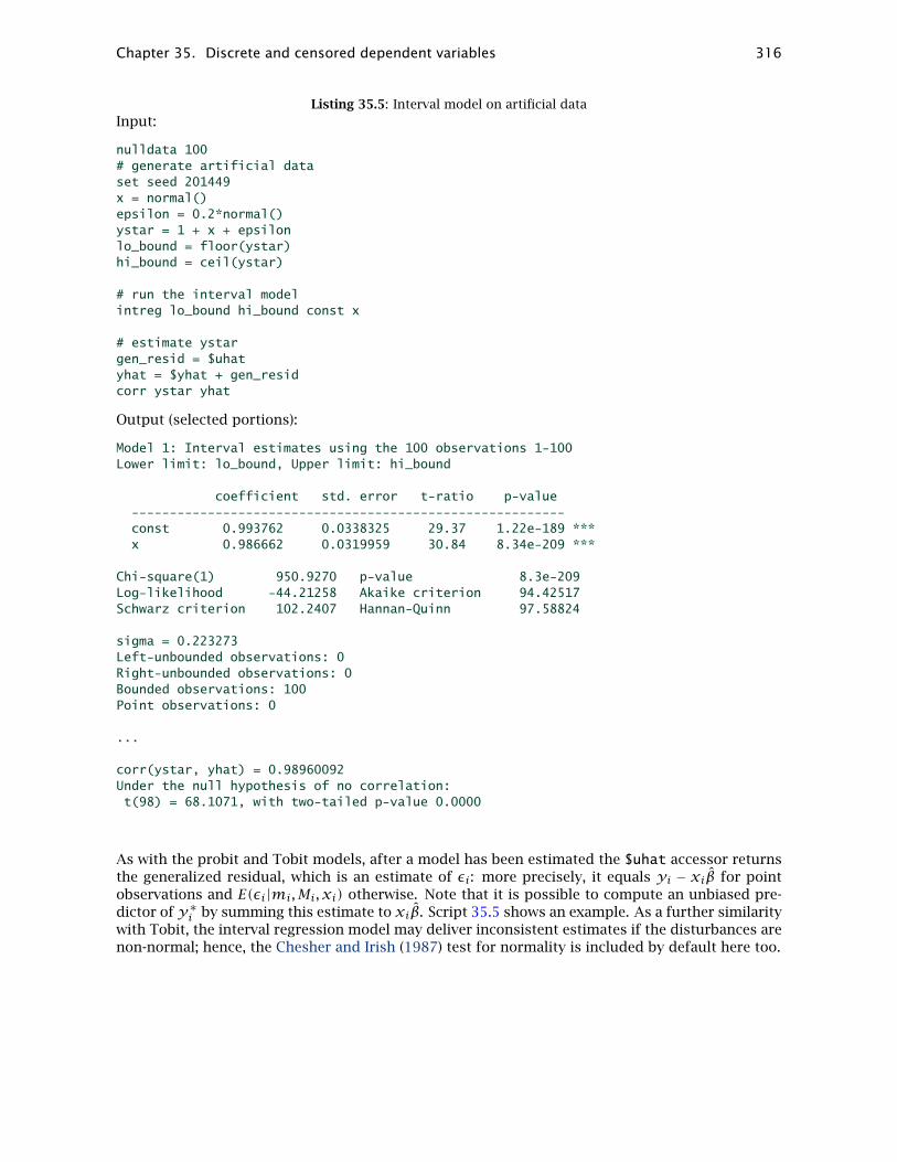
Chapter 35. Discrete and censored dependent variables 316
Listing 35.5: Interval model on artificial dataInput:
nulldata 100# generate artificial dataset seed 201449x = normal()epsilon = 0.2*normal()ystar = 1 + x + epsilonlo_bound = floor(ystar)hi_bound = ceil(ystar)
# run the interval modelintreg lo_bound hi_bound const x
# estimate ystargen_resid = $uhatyhat = $yhat + gen_residcorr ystar yhat
Output (selected portions):
Model 1: Interval estimates using the 100 observations 1-100Lower limit: lo_bound, Upper limit: hi_bound
coefficient std. error t-ratio p-value---------------------------------------------------------const 0.993762 0.0338325 29.37 1.22e-189 ***x 0.986662 0.0319959 30.84 8.34e-209 ***
Chi-square(1) 950.9270 p-value 8.3e-209Log-likelihood -44.21258 Akaike criterion 94.42517Schwarz criterion 102.2407 Hannan-Quinn 97.58824
sigma = 0.223273Left-unbounded observations: 0Right-unbounded observations: 0Bounded observations: 100Point observations: 0
...
corr(ystar, yhat) = 0.98960092Under the null hypothesis of no correlation:t(98) = 68.1071, with two-tailed p-value 0.0000
As with the probit and Tobit models, after a model has been estimated the $uhat accessor returnsthe generalized residual, which is an estimate of εi: more precisely, it equals yi − xiβ for pointobservations and E(εi|mi,Mi, xi) otherwise. Note that it is possible to compute an unbiased pre-dictor of y∗i by summing this estimate to xiβ. Script 35.5 shows an example. As a further similaritywith Tobit, the interval regression model may deliver inconsistent estimates if the disturbances arenon-normal; hence, the Chesher and Irish (1987) test for normality is included by default here too.

Chapter 35. Discrete and censored dependent variables 317
35.8 Sample selection model
In the sample selection model (also known as “Tobit II” model), there are two latent variables:
y∗i =k∑j=1
xijβj + εi (35.14)
s∗i =p∑j=1
zijγj + ηi (35.15)
and the observation rule is given by
yi =y∗i for s∗i > 0
♦ for s∗i ≤ 0(35.16)
In this context, the ♦ symbol indicates that for some observations we simply do not have data ony : yi may be 0, or missing, or anything else. A dummy variable di is normally used to set censoredobservations apart.
One of the most popular applications of this model in econometrics is a wage equation coupledwith a labor force participation equation: we only observe the wage for the employed. If y∗i and s∗iwere (conditionally) independent, there would be no reason not to use OLS for estimating equation(35.14); otherwise, OLS does not yield consistent estimates of the parameters βj .
Since conditional independence between y∗i and s∗i is equivalent to conditional independence be-tween εi and ηi, one may model the co-dependence between εi and ηi as
εi = ληi + vi;
substituting the above expression in (35.14), you obtain the model that is actually estimated:
yi =k∑j=1
xijβj + ληi + vi,
so the hypothesis that censoring does not matter is equivalent to the hypothesis H0 : λ = 0, whichcan be easily tested.
The parameters can be estimated via maximum likelihood under the assumption of joint normalityof εi and ηi; however, a widely used alternative method yields the so-called Heckit estimator, namedafter Heckman (1979). The procedure can be briefly outlined as follows: first, a probit model is fiton equation (35.15); next, the generalized residuals are inserted in equation (35.14) to correct forthe effect of sample selection.
Gretl provides the heckit command to carry out estimation; its syntax is
heckit y X ; d Z
where y is the dependent variable, X is a list of regressors, d is a dummy variable holding 1 foruncensored observations and Z is a list of explanatory variables for the censoring equation.
Since in most cases maximum likelihood is the method of choice, by default gretl computes MLestimates. The 2-step Heckit estimates can be obtained by using the --two-step option. Afterestimation, the $uhat accessor contains the generalized residuals. As in the ordinary Tobit model,the residuals equal the difference between actual and fitted yi only for uncensored observations(those for which di = 1).
Listing 35.6 shows two estimates from the dataset used in Mroz (1987): the first one replicatesTable 22.7 in Greene (2003),3 while the second one replicates table 17.1 in Wooldridge (2002a).
3Note that the estimates given by gretl do not coincide with those found in the printed volume. They do, however,match those found on the errata web page for Greene’s book: http://pages.stern.nyu.edu/~wgreene/Text/Errata/ERRATA5.htm.

Chapter 35. Discrete and censored dependent variables 318
Listing 35.6: Heckit model
open mroz87.gdt
genr EXP2 = AX^2genr WA2 = WA^2genr KIDS = (KL6+K618)>0
# Greene’s specification
list X = const AX EXP2 WE CITlist Z = const WA WA2 FAMINC KIDS WE
heckit WW X ; LFP Z --two-stepheckit WW X ; LFP Z
# Wooldridge’s specification
series NWINC = FAMINC - WW*WHRSseries lww = log(WW)list X = const WE AX EXP2list Z = X NWINC WA KL6 K618
heckit lww X ; LFP Z --two-step
35.9 Count data
Here the dependent variable is assumed to be a non-negative integer, so a probabilistic descriptionof yi|xi must hinge on some discrete distribution. The most common model is the Poisson model,in which
P(yi = Y |xi) = eµiµYiY !
µi = exp
∑jxijβj
In some cases, an “offset” variable is needed. The number of occurrences of yi in a given time isassumed to be strictly proportional to the offset variable ni. In the epidemiology literature, theoffset is known as “population at risk”. In this case, the model becomes
µi = ni exp
∑jxijβj
Another way to look at the offset variable is to consider its natural log as just another explanatoryvariable whose coefficient is constrained to be one.
Estimation is carried out by maximum likelihood and follows the syntax
poisson depvar indep
If an offset variable is needed, it has to be specified at the end of the command, separated from thelist of explanatory variables by a semicolon, as in
poisson depvar indep ; offset

Chapter 35. Discrete and censored dependent variables 319
It should be noted that the poisson command does not use, internally, the same optimizationengines as most other gretl command, such as arma or tobit. As a consequence, some details maydiffer: the --verbose option will yield different output and settings such as bfgs_toler will notwork.
Overdispersion
In the Poisson model, E(yi|xi) = V(yi|xi) = µi, that is, the conditional mean equals the conditionalvariance by construction. In many cases, this feature is at odds with the data, as the conditionalvariance is often larger than the mean; this phenomenon is called “overdispersion”. The outputfrom the poisson command includes a conditional moment test for overdispersion (as per David-son and MacKinnon (2004), section 11.5), which is printed automatically after estimation.
Overdispersion can be attributed to unmodeled heterogeneity between individuals. Two data pointswith the same observable characteristics xi = xj may differ because of some unobserved scalefactor si 6= sj so that
E(yi|xi, si) = µisi 6= µjsj = E(yj|xj , sj)even though µi = µj . In other words, yi is a Poisson random variable conditional on both xi and si,but since si is unobservable, the only thing we can we can use, P(yi|xi), will not follow the Poissondistribution.
It is often assumed that si can be represented as a gamma random variable with mean 1 andvariance α: the parameter α is estimated together with the vector β, and measures the degree ofheterogeneity between individuals.
In this case, the conditional probability for yi given xi can be shown to be
P(yi|xi) =Γ(yi +α−1)Γ(α−1)Γ(yi + 1)
[µi
µi +α−1
]yi [ α−1
µi +α−1
]α−1
(35.17)
which is known as the “Negative Binomial Model”. The conditional mean is still E(yi|xi) = µi, butthe variance equals V(yi|xi) = µi (1+ µiα). The gretl command for this model is negbin depvarindep.
• There is also a less used variant of the negative binomial model, in which the conditional vari-ance is a scalar multiple of the conditional mean, that is V(yi|xi) = µi (1+ γ). To distinguishbetween the two, the model (35.17) is termed “Type 2”. Gretl implements model 1 via theoption --model1.
• A script which exemplifies the above models is included among gretl’s sample scripts, underthe name camtriv.inp.
FIXME: expand.
35.10 Duration models
In some contexts we wish to apply econometric methods to measurements of the duration of certainstates. Classic examples include the following:
• From engineering, the “time to failure” of electronic or mechanical components: how long do,say, computer hard drives last until they malfunction?
• From the medical realm: how does a new treatment affect the time from diagnosis of a certaincondition to exit from that condition (where “exit” might mean death or full recovery)?
• From economics: the duration of strikes, or of spells of unemployment.

Chapter 35. Discrete and censored dependent variables 320
In each case we may be interested in how the durations are distributed, and how they are affectedby relevant covariates. There are several approaches to this problem; the one we discuss here—which is currently the only one supported by gretl—is estimation of a parametric model by meansof Maximum Likelihood. In this approach we hypothesize that the durations follow some definiteprobability law and we seek to estimate the parameters of that law, factoring in the influence ofcovariates.
We may express the density (PDF) of the durations as f(t,X, θ), where t is the length of time in thestate in question, X is a matrix of covariates, and θ is a vector of parameters. The likelihood for asample of n observations indexed by i is then
L =n∏i=1
f(ti, xi, θ)
Rather than working with the density directly, however, it is standard practice to factor f(·) intotwo components, namely a hazard function, λ, and a survivor function, S. The survivor functiongives the probability that a state lasts at least as long as t; it is therefore 1 − F(t,X, θ) where Fis the CDF corresponding to the density f(·). The hazard function addresses this question: giventhat a state has persisted as long as t, what is the likelihood that it ends within a short incrementof time beyond t—that is, it ends between t and t +∆? Taking the limit as ∆ goes to zero, we endup with the ratio of the density to the survivor function:4
λ(t,X, θ) = f(t,X, θ)S(t,X, θ)
(35.18)
so the log-likelihood can be written as
` =n∑i=1
logf(ti, xi, θ) =n∑i=1
logλ(ti, xi, θ)+ logS(ti, xi, θ) (35.19)
One point of interest is the shape of the hazard function, in particular its dependence (or not) ontime since the state began. If λ does not depend on t we say the process in question exhibits du-ration independence: the probability of exiting the state at any given moment neither increases nordecreases based simply on how long the state has persisted to date. The alternatives are positiveduration dependence (the likelihood of exiting the state rises, the longer the state has persisted)or negative duration dependence (exit becomes less likely, the longer it has persisted). Finally, thebehavior of the hazard with respect to time need not be monotonic; some parameterizations allowfor this possibility and some do not.
Since durations are inherently positive the probability distribution used in modeling must respectthis requirement, giving a density of zero for t ≤ 0. Four common candidates are the exponential,Weibull, log-logistic and log-normal, the Weibull being the most common choice. The table belowdisplays the density and the hazard function for each of these distributions as they are commonlyparameterized, written as functions of t alone. (φ and Φ denote, respectively, the Gaussian PDFand CDF.)
density, f(t) hazard, λ(t)
Exponential γ exp (−γt) γ
Weibull αγαtα−1 exp [−(γt)α] αγαtα−1
Log-logistic γα(γt)α−1
[1+ (γt)α]2γα
(γt)α−1
[1+ (γt)α]
Log-normal1σtφ[(log t − µ)/σ
] 1σt
φ[(log t − µ)/σ
]Φ [−(log t − µ)/σ
]4For a fuller discussion see, for example, Davidson and MacKinnon (2004).

Chapter 35. Discrete and censored dependent variables 321
The hazard is constant for the exponential distribution. For the Weibull, it is monotone increasingin t if α > 1, or monotone decreasing for α < 1. (If α = 1 the Weibull collapses to the exponential.)The log-logistic and log-normal distributions allow the hazard to vary with t in a non-monotonicfashion.
Covariates are brought into the picture by allowing them to govern one of the parameters of thedensity, so that durations are not identically distributed across cases. For example, when usingthe log-normal distribution it is natural to make µ, the expected value of log t, depend on thecovariates, X. This is typically done via a linear index function: µ = Xβ.
Note that the expressions for the log-normal density and hazard contain the term (log t − µ)/σ .Replacing µ with Xβ this becomes (log t −Xβ)/σ . As in Kalbfleisch and Prentice (2002), we definea shorthand label for this term:
wi ≡ (log ti − xiβ)/σ (35.20)
It turns out that this constitutes a useful simplifying change of variables for all of the distributionsdiscussed here. The interpretation of the scale factor, σ , in the expression above depends on thedistribution. For the log-normal, σ represents the standard deviation of log t; for the Weibull andthe log-logistic it corresponds to 1/α; and for the exponential it is fixed at unity. For distributionsother than the log-normal, Xβ corresponds to − logγ, or in other words γ = exp(−Xβ).With this change of variables, the density and survivor functions may be written compactly asfollows (the exponential is the same as the Weibull).
density, f(wi) survivor, S(wi)
Weibull exp (wi − ewi) exp(−ewi)
Log-logistic ewi (1+ ewi)−2 (1+ ewi)−1
Log-normal φ(wi) Φ(−wi)In light of the above we may think of the generic parameter vector θ, as in f(t,X, θ), as composed ofthe coefficients on the covariates, β, plus (in all cases but the exponential) the additional parameterσ .
A complication in estimation of θ is posed by “incomplete spells”. That is, in some cases the statein question may not have ended at the time the observation is made (e.g. some workers remainunemployed, some components have not yet failed). If we use ti to denote the time from enteringthe state to either (a) exiting the state or (b) the observation window closing, whichever comes first,then all we know of the “right-censored” cases (b) is that the duration was at least as long as ti.This can be handled by rewriting the the log-likelihood (compare 35.19) as
`i =n∑i=1
δi logS (wi)+ (1− δi)[− logσ + logf (wi)
](35.21)
where δi equals 1 for censored cases (incomplete spells), and 0 for complete observations. Therationale for this is that the log-density equals the sum of the log hazard and the log survivorfunction, but for the incomplete spells only the survivor function contributes to the likelihood. Soin (35.21) we are adding up the log survivor function alone for the incomplete cases, plus the fulllog density for the completed cases.
Implementation in gretl and illustration
The duration command accepts a list of series on the usual pattern: dependent variable followedby covariates. If right-censoring is present in the data this should be represented by a dummyvariable corresponding to δi above, separated from the covariates by a semicolon. For example,
duration durat 0 X ; cens

Chapter 35. Discrete and censored dependent variables 322
where durat measures durations, 0 represents the constant (which is required for such models), Xis a named list of regressors, and cens is the censoring dummy.
By default the Weibull distribution is used; you can substitute any of the other three distribu-tions discussed here by appending one of the option flags --exponential, --loglogistic or--lognormal.
Interpreting the coefficients in a duration model requires some care, and we will work throughan illustrative case. The example comes from section 20.3 of Wooldridge (2002a) and it concernscriminal recidivism.5 The data (filename recid.gdt) pertain to a sample of 1,445 convicts releasedfrom prison between July 1, 1977 and June 30, 1978. The dependent variable is the time in monthsuntil they are again arrested. The information was gathered retrospectively by examining recordsin April 1984; the maximum possible length of observation is 81 months. Right-censoring is impor-tant: when the date were compiled about 62 percent had not been rearrested. The dataset containsseveral covariates, which are described in the data file; we will focus below on interpretation of themarried variable, a dummy which equals 1 if the respondent was married when imprisoned.
Listing 35.7 shows the gretl commands for Weibull and log-normal models along with most of theoutput. Consider first the Weibull scale factor, σ . The estimate is 1.241 with a standard error of0.048. (We don’t print a z score and p-value for this term since H0 : σ = 0 is not of interest.)Recall that σ corresponds to 1/α; we can be confident that α is less than 1, so recidivism displaysnegative duration dependence. This makes sense: it is plausible that if a past offender managesto stay out of trouble for an extended period his risk of engaging in crime again diminishes. (Theexponential model would therefore not be appropriate in this case.)
On a priori grounds, however, we may doubt the monotonic decline in hazard that is implied bythe Weibull specification. Even if a person is liable to return to crime, it seems relatively unlikelythat he would do so straight out of prison. In the data, we find that only 2.6 percent of thosefollowed were rearrested within 3 months. The log-normal specification, which allows the hazardto rise and then fall, may be more appropriate. Using the duration command again with the samecovariates but the --lognormal flag, we get a log-likelihood of −1597 as against −1633 for theWeibull, confirming that the log-normal gives a better fit.
Let us now focus on the married coefficient, which is positive in both specifications but larger andmore sharply estimated in the log-normal variant. The first thing is to get the interpretation of thesign right. Recall that Xβ enters negatively into the intermediate variable w (equation 35.20). TheWeibull hazard is λ(wi) = ewi , so being married reduces the hazard of re-offending, or in otherwords lengthens the expected duration out of prison. The same qualitative interpretation appliesfor the log-normal.
To get a better sense of the married effect, it is useful to show its impact on the hazard across time.We can do this by plotting the hazard for two values of the index function Xβ: in each case thevalues of all the covariates other than married are set to their means (or some chosen values) whilemarried is set first to 0 then to 1. Listing 35.8 provides a script that does this, and the resultingplots are shown in Figure 35.1. Note that when computing the hazards we need to multiply by theJacobian of the transformation from ti to wi = log(ti − xiβ)/σ , namely 1/t. Note also that theestimate of σ is available via the accessor $sigma, but it is also present as the last element in thecoefficient vector obtained via $coeff.
A further difference between the Weibull and log-normal specifications is illustrated in the plots.The Weibull is an instance of a proportional hazard model. This means that for any sets of values ofthe covariates, xi and xj , the ratio of the associated hazards is invariant with respect to duration. Inthis example the Weibull hazard for unmarried individuals is always 1.1637 times that for married.In the log-normal variant, on the other hand, this ratio gradually declines from 1.6703 at one monthto 1.1766 at 100 months.
5Germán Rodríguez of Princeton University has a page discussing this example and displaying estimates from Stataat http://data.princeton.edu/pop509/recid1.html.

Chapter 35. Discrete and censored dependent variables 323
Listing 35.7: Models for recidivism dataInput:
open recid.gdtlist X = workprg priors tserved felon alcohol drugs \black married educ age
duration durat 0 X ; censduration durat 0 X ; cens --lognormal
Partial output:
Model 1: Duration (Weibull), using observations 1-1445Dependent variable: durat
coefficient std. error z p-value--------------------------------------------------------const 4.22167 0.341311 12.37 3.85e-35 ***workprg -0.112785 0.112535 -1.002 0.3162priors -0.110176 0.0170675 -6.455 1.08e-10 ***tserved -0.0168297 0.00213029 -7.900 2.78e-15 ***felon 0.371623 0.131995 2.815 0.0049 ***alcohol -0.555132 0.132243 -4.198 2.69e-05 ***drugs -0.349265 0.121880 -2.866 0.0042 ***black -0.563016 0.110817 -5.081 3.76e-07 ***married 0.188104 0.135752 1.386 0.1659educ 0.0289111 0.0241153 1.199 0.2306age 0.00462188 0.000664820 6.952 3.60e-12 ***sigma 1.24090 0.0482896
Chi-square(10) 165.4772 p-value 2.39e-30Log-likelihood -1633.032 Akaike criterion 3290.065
Model 2: Duration (log-normal), using observations 1-1445Dependent variable: durat
coefficient std. error z p-value---------------------------------------------------------const 4.09939 0.347535 11.80 4.11e-32 ***workprg -0.0625693 0.120037 -0.5213 0.6022priors -0.137253 0.0214587 -6.396 1.59e-10 ***tserved -0.0193306 0.00297792 -6.491 8.51e-11 ***felon 0.443995 0.145087 3.060 0.0022 ***alcohol -0.634909 0.144217 -4.402 1.07e-05 ***drugs -0.298159 0.132736 -2.246 0.0247 **black -0.542719 0.117443 -4.621 3.82e-06 ***married 0.340682 0.139843 2.436 0.0148 **educ 0.0229194 0.0253974 0.9024 0.3668age 0.00391028 0.000606205 6.450 1.12e-10 ***sigma 1.81047 0.0623022
Chi-square(10) 166.7361 p-value 1.31e-30Log-likelihood -1597.059 Akaike criterion 3218.118

Chapter 35. Discrete and censored dependent variables 324
Listing 35.8: Create plots showing conditional hazards
open recid.gdt -q
# leave ’married’ separate for analysislist X = workprg priors tserved felon alcohol drugs \black educ age
# Weibull variantduration durat 0 X married ; cens# coefficients on all Xs apart from marriedmatrix beta_w = $coeff[1:$ncoeff-2]# married coefficientscalar mc_w = $coeff[$ncoeff-1]scalar s_w = $sigma
# Log-normal variantduration durat 0 X married ; cens --lognormalmatrix beta_n = $coeff[1:$ncoeff-2]scalar mc_n = $coeff[$ncoeff-1]scalar s_n = $sigma
list allX = 0 X# evaluate X\beta at means of all variables except marriagescalar Xb_w = meanc(allX) * beta_wscalar Xb_n = meanc(allX) * beta_n
# construct two plot matricesmatrix mat_w = zeros(100, 3)matrix mat_n = zeros(100, 3)
loop t=1..100 -q# first column, durationmat_w[t, 1] = tmat_n[t, 1] = twi_w = (log(t) - Xb_w)/s_wwi_n = (log(t) - Xb_n)/s_n# second col: hazard with married = 0mat_w[t, 2] = (1/t) * exp(wi_w)mat_n[t, 2] = (1/t) * pdf(z, wi_n) / cdf(z, -wi_n)wi_w = (log(t) - (Xb_w + mc_w))/s_wwi_n = (log(t) - (Xb_n + mc_n))/s_n# third col: hazard with married = 1mat_w[t, 3] = (1/t) * exp(wi_w)mat_n[t, 3] = (1/t) * pdf(z, wi_n) / cdf(z, -wi_n)
endloop
colnames(mat_w, "months unmarried married")colnames(mat_n, "months unmarried married")
gnuplot 2 3 1 --with-lines --supp --matrix=mat_w --output=weibull.pltgnuplot 2 3 1 --with-lines --supp --matrix=mat_n --output=lognorm.plt

Chapter 35. Discrete and censored dependent variables 325
0.006
0.008
0.010
0.012
0.014
0.016
0.018
0.020
0 20 40 60 80 100
months
Weibull
unmarriedmarried
0.006
0.008
0.010
0.012
0.014
0.016
0.018
0.020
0 20 40 60 80 100
months
Log-normal
unmarriedmarried
Figure 35.1: Recidivism hazard estimates for married and unmarried ex-convicts

Chapter 35. Discrete and censored dependent variables 326
Alternative representations of the Weibull model
One point to watch out for with the Weibull duration model is that the estimates may be representedin different ways. The representation given by gretl is sometimes called the accelerated failure-time(AFT) metric. An alternative that one sometimes sees is the log relative-hazard metric; in fact this isthe metric used in Wooldridge’s presentation of the recidivism example. To get from AFT estimatesto log relative-hazard form it is necessary to multiply the coefficients by −σ−1. For example, themarried coefficient in the Weibull specification as shown here is 0.188104 and σ is 1.24090, so thealternative value is −0.152, which is what Wooldridge shows (2002a, Table 20.1).
Fitted values and residuals
By default, gretl computes fitted values (accessible via $yhat) as the conditional mean of duration.The formulae are shown below (where Γ denotes the gamma function, and the exponential variantis just Weibull with σ = 1).
Weibull Log-logistic Log-normal
exp(Xβ)Γ(1+ σ) exp(Xβ)πσ
sin(πσ)exp(Xβ+ σ 2/2)
The expression given for the log-logistic mean, however, is valid only for σ < 1; otherwise theexpectation is undefined, a point that is not noted in all software.6
Alternatively, if the --medians option is given, gretl’s duration command will produce conditionalmedians as the content of $yhat. For the Weibull the median is exp(Xβ)(log 2)σ ; for the log-logisticand log-normal it is just exp(Xβ).
The values we give for the accessor $uhat are generalized (Cox–Snell) residuals, computed as theintegrated hazard function, which equals the negative log of the survivor function:
εi = Λ(ti, xi, θ) = − logS(ti, xi, θ)
Under the null of correct specification of the model these generalized residuals should follow theunit exponential distribution, which has mean and variance both equal to 1 and density exp(−ε).See chapter 18 of Cameron and Trivedi (2005) for further discussion.
6The predict adjunct to the streg command in Stata 10, for example, gaily produces large negative values for thelog-logistic mean in duration models with σ > 1.
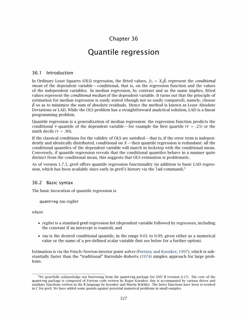
Chapter 36
Quantile regression
36.1 Introduction
In Ordinary Least Squares (OLS) regression, the fitted values, yi = Xiβ, represent the conditionalmean of the dependent variable—conditional, that is, on the regression function and the valuesof the independent variables. In median regression, by contrast and as the name implies, fittedvalues represent the conditional median of the dependent variable. It turns out that the principle ofestimation for median regression is easily stated (though not so easily computed), namely, chooseβ so as to minimize the sum of absolute residuals. Hence the method is known as Least AbsoluteDeviations or LAD. While the OLS problem has a straightforward analytical solution, LAD is a linearprogramming problem.
Quantile regression is a generalization of median regression: the regression function predicts theconditional τ-quantile of the dependent variable—for example the first quartile (τ = .25) or theninth decile (τ = .90).
If the classical conditions for the validity of OLS are satisfied—that is, if the error term is indepen-dently and identically distributed, conditional on X—then quantile regression is redundant: all theconditional quantiles of the dependent variable will march in lockstep with the conditional mean.Conversely, if quantile regression reveals that the conditional quantiles behave in a manner quitedistinct from the conditional mean, this suggests that OLS estimation is problematic.
As of version 1.7.5, gretl offers quantile regression functionality (in addition to basic LAD regres-sion, which has been available since early in gretl’s history via the lad command).1
36.2 Basic syntax
The basic invocation of quantile regression is
quantreg tau reglist
where
• reglist is a standard gretl regression list (dependent variable followed by regressors, includingthe constant if an intercept is wanted); and
• tau is the desired conditional quantile, in the range 0.01 to 0.99, given either as a numericalvalue or the name of a pre-defined scalar variable (but see below for a further option).
Estimation is via the Frisch–Newton interior point solver (Portnoy and Koenker, 1997), which is sub-stantially faster than the “traditional” Barrodale–Roberts (1974) simplex approach for large prob-lems.
1We gratefully acknowledge our borrowing from the quantreg package for GNU R (version 4.17). The core of thequantreg package is composed of Fortran code written by Roger Koenker; this is accompanied by various driver andauxiliary functions written in the R language by Koenker and Martin Mächler. The latter functions have been re-workedin C for gretl. We have added some guards against potential numerical problems in small samples.
327

Chapter 36. Quantile regression 328
By default, standard errors are computed according to the asymptotic formula given by Koenkerand Bassett (1978). Alternatively, if the --robust option is given, we use the sandwich estimatordeveloped in Koenker and Zhao (1994).2
36.3 Confidence intervals
An option --intervals is available. When this is given we print confidence intervals for the param-eter estimates instead of standard errors. These intervals are computed using the rank inversionmethod and in general they are asymmetrical about the point estimates—that is, they are not sim-ply “plus or minus so many standard errors”. The specifics of the calculation are inflected bythe --robust option: without this, the intervals are computed on the assumption of IID errors(Koenker, 1994); with it, they use the heteroskedasticity-robust estimator developed by Koenkerand Machado (1999).
By default, 90 percent intervals are produced. You can change this by appending a confidence value(expressed as a decimal fraction) to the intervals option, as in
quantreg tau reglist --intervals=.95
When the confidence intervals option is selected, the parameter estimates are calculated usingthe Barrodale–Roberts method. This is simply because the Frisch–Newton code does not currentlysupport the calculation of confidence intervals.
Two further details. First, the mechanisms for generating confidence intervals for quantile esti-mates require that the model has at least two regressors (including the constant). If the --intervalsoption is given for a model containing only one regressor, an error is flagged. Second, when a modelis estimated in this mode, you can retrieve the confidence intervals using the accessor $coeff_ci.This produces a k × 2 matrix, where k is the number of regressors. The lower bounds are in thefirst column, the upper bounds in the second. See also section 36.5 below.
36.4 Multiple quantiles
As a further option, you can give tau as a matrix—either the name of a predefined matrix or innumerical form, as in .05, .25, .5, .75, .95. The given model is estimated for all the τvalues and the results are printed in a special form, as shown below (in this case the --intervalsoption was also given).
Model 1: Quantile estimates using the 235 observations 1-235Dependent variable: foodexpWith 90 percent confidence intervals
VARIABLE TAU COEFFICIENT LOWER UPPER
const 0.05 124.880 98.3021 130.5170.25 95.4835 73.7861 120.0980.50 81.4822 53.2592 114.0120.75 62.3966 32.7449 107.3140.95 64.1040 46.2649 83.5790
income 0.05 0.343361 0.343327 0.3897500.25 0.474103 0.420330 0.4943290.50 0.560181 0.487022 0.6019890.75 0.644014 0.580155 0.6904130.95 0.709069 0.673900 0.734441
2These correspond to the iid and nid options in R’s quantreg package, respectively.
Chapter 36. Quantile regression 329
0.3
0.35
0.4
0.45
0.5
0.55
0.6
0.65
0.7
0.75
0 0.2 0.4 0.6 0.8 1
tau
Coefficient on income
Quantile estimates with 90% bandOLS estimate with 90% band
Figure 36.1: Regression of food expenditure on income; Engel’s data
The gretl GUI has an entry for Quantile Regression (under /Model/Robust estimation), and you canselect multiple quantiles there too. In that context, just give space-separated numerical values (asper the predefined options, shown in a drop-down list).
When you estimate a model in this way most of the standard menu items in the model windoware disabled, but one extra item is available—graphs showing the τ sequence for a given coeffi-cient in comparison with the OLS coefficient. An example is shown in Figure 36.1. This sort ofgraph provides a simple means of judging whether quantile regression is redundant (OLS is fine) orinformative.
In the example shown—based on data on household income and food expenditure gathered byErnst Engel (1821–1896)—it seems clear that simple OLS regression is potentially misleading. The“crossing” of the OLS estimate by the quantile estimates is very marked.
However, it is not always clear what implications should be drawn from this sort of conflict. Withthe Engel data there are two issues to consider. First, Engel’s famous “law” claims an income-elasticity of food consumption that is less than one, and talk of elasticities suggests a logarithmicformulation of the model. Second, there are two apparently anomalous observations in the dataset: household 105 has the third-highest income but unexpectedly low expenditure on food (asjudged from a simple scatter plot), while household 138 (which also has unexpectedly low foodconsumption) has much the highest income, almost twice that of the next highest.
With n = 235 it seems reasonable to consider dropping these observations. If we do so, and adopta log–log formulation, we get the plot shown in Figure 36.2. The quantile estimates still cross theOLS estimate, but the “evidence against OLS” is much less compelling: the 90 percent confidencebands of the respective estimates overlap at all the quantiles considered.
36.5 Large datasets
As noted above, when you give the --intervals option with the quantreg command, which callsfor estimation of confidence intervals via rank inversion, gretl switches from the default Frisch–Newton algorithm to the Barrodale–Roberts simplex method.

Chapter 36. Quantile regression 330
0.76
0.78
0.8
0.82
0.84
0.86
0.88
0.9
0.92
0.94
0.96
0 0.2 0.4 0.6 0.8 1
tau
Coefficient on log(income)
Quantile estimates with 90% bandOLS estimate with 90% band
Figure 36.2: Log–log regression; 2 observations dropped from full Engel data set.
This is OK for moderately large datasets (up to, say, a few thousand observations) but on very largeproblems the simplex algorithm may become seriously bogged down. For example, Koenker andHallock (2001) present an analysis of the determinants of birth weights, using 198377 observationsand with 15 regressors. Generating confidence intervals via Barrodale–Roberts for a single value ofτ took about half an hour on a Lenovo Thinkpad T60p with 1.83GHz Intel Core 2 processor.
If you want confidence intervals in such cases, you are advised not to use the --intervals option,but to compute them using the method of “plus or minus so many standard errors”. (One Frisch–Newton run took about 8 seconds on the same machine, showing the superiority of the interiorpoint method.) The script below illustrates:
quantreg .10 y 0 xlistscalar crit = qnorm(.95)matrix ci = $coeff - crit * $stderrci = ci~($coeff + crit * $stderr)print ci
The matrix ci will contain the lower and upper bounds of the (symmetrical) 90 percent confidenceintervals.
To avoid a situation where gretl becomes unresponsive for a very long time we have set the maxi-mum number of iterations for the Borrodale–Roberts algorithm to the (somewhat arbitrary) valueof 1000. We will experiment further with this, but for the meantime if you really want to use thismethod on a large dataset, and don’t mind waiting for the results, you can increase the limit usingthe set command with parameter rq_maxiter, as in
set rq_maxiter 5000

Chapter 37
Nonparametric methods
The main focus of gretl is on parametric estimation, but we offer a selection of nonparametricmethods. The most basic of these
• various tests for difference in distribution (Sign test, Wilcoxon rank-sum test, Wilcoxon signed-rank test);
• the Runs test for randomness; and
• nonparametric measures of association: Spearman’s rho and Kendall’s tau.
Details on the above can be found by consulting the help for the commands difftest, runs, corrand spearman. In the GUI program these items are found under the Tools menu and the Robustestimation item under the Model menu.
In this chapter we concentrate on two relatively complex methods for nonparametric curve-fittingand prediction, namely William Cleveland’s “loess” (also known as “lowess”) and the Nadaraya–Watson estimator.
37.1 Locally weighted regression (loess)
Loess (Cleveland, 1979) is a nonparametric smoother employing locally weighted polynomial re-gression. It is intended to yield an approximation to g(·) when the dependent variable, y , can beexpressed as
yi = g(xi)+ εifor some smooth function g(·).Given a sample of n observations on the variables y and x, the procedure is to run a weighted leastsquares regression (a polynomial of order d = 0, 1 or 2 in x) localized to each data point, i. In eachsuch regression the sample consists of the r nearest neighbors (in the x dimension) to the point i,with weights that are inversely related to the distance |xi − xk|, k = 1, . . . , r . The predicted valueyi is then obtained by evaluating the estimated polynomial at xi. The most commonly used orderis d = 1.
A bandwidth parameter 0 < q ≤ 1 controls the proportion of the total number of data points usedin each regression; thus r = qn (rounded up to an integer). Larger values of q lead to a smootherfitted series, smaller values to a series that tracks the actual data more closely; 0.25 ≤ q ≤ 0.5 isoften a suitable range.
In gretl’s implementation of loess the weighting scheme is that given by Cleveland, namely,
wk(xi) = W(h−1i (xk − xi))
where hi is the distance between xi and its r th nearest neighbor, and W(·) is the tricube function,
W(x) =(1− |x|3)3 for |x| < 1
0 for |x| ≥ 1
331

Chapter 37. Nonparametric methods 332
The local regression can be made robust via an adjustment based on the residuals, ei = yi − yi.Robustness weights, δk, are defined by
δk = B(ek/6s)
where s is the median of the |ei| and B(·) is the bisquare function,
B(x) =(1− x2)2 for |x| < 1
0 for |x| ≥ 1
The polynomial regression is then re-run using weight δkwk(xi) at (xk, yk).
The loess() function in gretl takes up to five arguments as follows: the y series, the x series, theorder d, the bandwidth q, and a Boolean switch to turn on the robust adjustment. The last threearguments are optional: if they are omitted the default values are d = 1, q = 0.5 and no robustadjustment. An example of a full call to loess() is shown below; in this case a quadratic in x isspecified, three quarters of the data points will be used in each local regression, and robustness isturned on:
series yh = loess(y, x, 2, 0.75, 1)
An illustration of loess is provided in Listing 37.1: we generate a series that has a deterministicsine wave component overlaid with noise uniformly distributed on (−1,1). Loess is then used toretrieve a good approximation to the sine function. The resulting graph is shown in Figure 37.1.
Listing 37.1: Loess script
nulldata 120series x = indexscalar n = $nobsseries y = sin(2*pi*x/n) + uniform(-1, 1)series yh = loess(y, x, 2, 0.75, 0)gnuplot y yh x --output=display --with-lines=yh
-2
-1.5
-1
-0.5
0
0.5
1
1.5
2
0 20 40 60 80 100 120
x
loess fit
Figure 37.1: Loess: retrieving a sine wave

Chapter 37. Nonparametric methods 333
37.2 The Nadaraya–Watson estimator
The Nadaraya–Watson nonparametric estimator (Nadaraya, 1964; Watson, 1964) is an estimatorfor the conditional mean of a variable Y , available in a sample of size n, for a given value of aconditioning variable X, and is defined as
m(X) =∑nj=1yj ·Kh(X − xj)∑nj=1Kh(X − xj)
where Kh(·) is the so-called kernel function, which is usually some simple transform of a densityfunction that depends on a scalar called the bandwidth. The one gretl uses is given by
Kh(x) = exp
(−x
2
2h
)
for |x| < τ and zero otherwise. The scalar τ is used to prevent numerical problems when thekernel function is evaluated too far away from zero and is called the trim parameter.
Listing 37.2: Nadaraya–Watson example
# Nonparametric regression example: husband’s age on wife’s ageopen mroz87.gdt
# initial value for the bandwidthscalar h = $nobs^(-0.2)# three increasingly smooth estimatesseries m0 = nadarwat(HA, WA, h)series m1 = nadarwat(HA, WA, h * 5)series m2 = nadarwat(HA, WA, h * 10)
# produce the graphdataset sortby WAgnuplot HA m0 m1 m2 WA --output=display --with-lines=m0,m1,m2
Listing 37.2 produces the graph shown in Figure 37.2 (after some slight editing).
The choice of the bandwidth is up to the user: larger values of h lead to a smootherm(·) function;smaller values make the m(·) function follow the yi values more closely, so that the functionappears more “jagged”. In fact, as h → ∞, m(xi) → Y ; on the contrary, if h → 0, observations forwhich xi 6= X are not taken into account at all when computing m(X).
Also, the statistical properties of m(·) vary with h: its variance can be shown to be decreasing inh, while its squared bias is increasing in h. It can be shown that choosing h ∼ n−1/5 minimizes theRMSE, so that value is customarily taken as a reference point.
Note that the kernel function has its tails “trimmed”. The scalar τ , which controls the level atwhich trimming occurs is set by default at 4 · h; this setting, however, may be changed via the setcommand. For example,
set nadarwat_trim 10
sets τ = 10 · h. This may at times produce more sensible results in regions of X with sparsesupport; however, you should be aware that in those same cases machine precision (division bynumerical zero) may render your results spurious. The default is relatively safe, but experimentingwith larger values may be a sensible strategy in some cases.
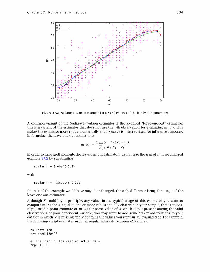
Chapter 37. Nonparametric methods 334
30
35
40
45
50
55
60
30 35 40 45 50 55 60
HA
WA
m0m1m2
Figure 37.2: Nadaraya–Watson example for several choices of the bandwidth parameter
A common variant of the Nadaraya–Watson estimator is the so-called “leave-one-out” estimator:this is a variant of the estimator that does not use the i-th observation for evaluating m(xi). Thismakes the estimator more robust numerically and its usage is often advised for inference purposes.In formulae, the leave-one-out estimator is
m(xi) =∑j 6=iyj ·Kh(xi − xj)∑j 6=iKh(xi − xj)
In order to have gretl compute the leave-one-out estimator, just reverse the sign of h: if we changedexample 37.2 by substituting
scalar h = $nobs^(-0.2)
with
scalar h = -($nobs^(-0.2))
the rest of the example would have stayed unchanged, the only difference being the usage of theleave-one-out estimator.
Although X could be, in principle, any value, in the typical usage of this estimator you want tocompute m(X) for X equal to one or more values actually observed in your sample, that is m(xi).If you need a point estimate of m(X) for some value of X which is not present among the validobservations of your dependent variable, you may want to add some “fake” observations to yourdataset in which y is missing and x contains the values you wantm(x) evaluated at. For example,the following script evaluates m(x) at regular intervals between -2.0 and 2.0:
nulldata 120set seed 120496
# first part of the sample: actual datasmpl 1 100

Chapter 37. Nonparametric methods 335
x = normal()y = x^2 + sin(x) + normal()
# second part of the sample: fake x datasmpl 101 120x = (obs-110) / 5
# compute the Nadaraya-Watson estimate# with bandwidth equal to 0.4 (note that# 100^(-0.2) = 0.398)smpl fullm = nadarwat(y, x, 0.4)
# show m(x) for the fake x values onlysmpl 101 120print x m -o
and running it produces
x m
101 -1.8 1.165934102 -1.6 0.730221103 -1.4 0.314705104 -1.2 0.026057105 -1.0 -0.131999106 -0.8 -0.215445107 -0.6 -0.269257108 -0.4 -0.304451109 -0.2 -0.306448110 0.0 -0.238766111 0.2 -0.038837112 0.4 0.354660113 0.6 0.908178114 0.8 1.485178115 1.0 2.000003116 1.2 2.460100117 1.4 2.905176118 1.6 3.380874119 1.8 3.927682120 2.0 4.538364

Part III
Technical details
336

Chapter 38
Gretl and TEX
38.1 Introduction
TEX — initially developed by Donald Knuth of Stanford University and since enhanced by hundredsof contributors around the world — is the gold standard of scientific typesetting. Gretl providesvarious hooks that enable you to preview and print econometric results using the TEX engine, andto save output in a form suitable for further processing with TEX.
This chapter explains the finer points of gretl’s TEX-related functionality. The next section describesthe relevant menu items; section 38.3 discusses ways of fine-tuning TEX output; and section 38.4gives some pointers on installing (and learning) TEX if you do not already have it on your computer.(Just to be clear: TEX is not included with the gretl distribution; it is a separate package, includingseveral programs and a large number of supporting files.)
Before proceeding, however, it may be useful to set out briefly the stages of production of a finaldocument using TEX. For the most part you don’t have to worry about these details, since, in regardto previewing at any rate, gretl handles them for you. But having some grasp of what is going onbehind the scences will enable you to understand your options better.
The first step is the creation of a plain text “source” file, containing the text or mathematics tobe typset, interspersed with mark-up that defines how it should be formatted. The second stepis to run the source through a processing engine that does the actual formatting. Typically this aprogram called pdflatex that generates PDF output.1 (In times gone by it was a program called latexthat generated so-called DVI (device-independent) output.)
So gretl calls pdflatex to process the source file. On MS Windows and Mac OS X, gretl expects theoperating system to find the default viewer for PDF output. On GNU/Linux you can specify yourpreferred PDF viewer via the menu item “Tools, Preferences, General,” under the “Programs” tab.
38.2 TEX-related menu items
The model window
The fullest TEX support in gretl is found in the GUI model window. This has a menu item titled“LaTeX” with sub-items “View”, “Copy”, “Save” and “Equation options” (see Figure 38.1).
The first three sub-items have branches titled “Tabular” and “Equation”. By “Tabular” we mean thatthe model is represented in the form of a table; this is the fullest and most explicit presentation ofthe results. See Table 38.1 for an example; this was pasted into the manual after using the “Copy,Tabular” item in gretl (a few lines were edited out for brevity).
The “Equation” option is fairly self-explanatory—the results are written across the page in equationformat, as below:
ÆENROLL = 0.241105(0.066022)
+ 0.223530(0.04597)
CATHOL− 0.00338200(0.0027196)
PUPIL− 0.152643(0.040706)
WHITE
T = 51 R2 = 0.4462 F(3,47) = 14.431 σ = 0.038856
1Experts will be aware of something called “plain TEX”, which is processed using the program tex. The great majorityof TEX users, however, use the LATEX macros, initially developed by Leslie Lamport. gretl does not support plain TEX.
337

Chapter 38. Gretl and TEX 338
Figure 38.1: LATEX menu in model window
Table 38.1: Example of LATEX tabular output
Model 1: OLS estimates using the 51 observations 1–51Dependent variable: ENROLL
Variable Coefficient Std. Error t-statistic p-value
const 0.241105 0.0660225 3.6519 0.0007
CATHOL 0.223530 0.0459701 4.8625 0.0000
PUPIL −0.00338200 0.00271962 −1.2436 0.2198
WHITE −0.152643 0.0407064 −3.7499 0.0005
Mean of dependent variable 0.0955686
S.D. of dependent variable 0.0522150
Sum of squared residuals 0.0709594
Standard error of residuals (σ ) 0.0388558
Unadjusted R2 0.479466
Adjusted R2 0.446241
F(3,47) 14.4306

Chapter 38. Gretl and TEX 339
(standard errors in parentheses)
The distinction between the “Copy” and “Save” options (for both tabular and equation) is twofold.First, “Copy” puts the TEX source on the clipboard while with “Save” you are prompted for the nameof a file into which the source should be saved. Second, with “Copy” the material is copied as a“fragment” while with “Save” it is written as a complete file. The point is that a well-formed TEXsource file must have a header that defines the documentclass (article, report, book or whatever)and tags that say \begindocument and \enddocument. This material is included when you do“Save” but not when you do “Copy”, since in the latter case the expectation is that you will pastethe data into an existing TEX source file that already has the relevant apparatus in place.
The items under “Equation options” should be self-explanatory: when printing the model in equa-tion form, do you want standard errors or t-ratios displayed in parentheses under the parameterestimates? The default is to show standard errors; if you want t-ratios, select that item.
Other windows
Several other sorts of output windows also have TEX preview, copy and save enabled. In the case ofwindows having a graphical toolbar, look for the TEX button. Figure 38.2 shows this icon (secondfrom the right on the toolbar) along with the dialog that appears when you press the button.
Figure 38.2: TEX icon and dialog
One aspect of gretl’s TEX support that is likely to be particularly useful for publication purposes isthe ability to produce a typeset version of the “model table” (see section 3.4). An example of this isshown in Table 38.2.
38.3 Fine-tuning typeset output
There are three aspects to this: adjusting the appearance of the output produced by gretl inLATEX preview mode; adjusting the formatting of gretl’s tabular output for models when using thetabprint command; and incorporating gretl’s output into your own TEX files.
Previewing in the GUI
As regards preview mode, you can control the appearance of gretl’s output using a file namedgretlpre.tex, which should be placed in your gretl user directory (see the Gretl Command Ref-erence). If such a file is found, its contents will be used as the “preamble” to the TEX source. Thedefault value of the preamble is as follows:
\documentclass[11pt]article\usepackage[utf8]inputenc

Chapter 38. Gretl and TEX 340
Table 38.2: Example of model table output
OLS estimatesDependent variable: ENROLL
Model 1 Model 2 Model 3
const 0.2907∗∗ 0.2411∗∗ 0.08557
(0.07853) (0.06602) (0.05794)
CATHOL 0.2216∗∗ 0.2235∗∗ 0.2065∗∗
(0.04584) (0.04597) (0.05160)
PUPIL −0.003035 −0.003382 −0.001697
(0.002727) (0.002720) (0.003025)
WHITE −0.1482∗∗ −0.1526∗∗
(0.04074) (0.04071)
ADMEXP −0.1551
(0.1342)
n 51 51 51
R2 0.4502 0.4462 0.2956
` 96.09 95.36 88.69
Standard errors in parentheses* indicates significance at the 10 percent level** indicates significance at the 5 percent level

Chapter 38. Gretl and TEX 341
\usepackageamsmath\usepackagedcolumn,longtable\begindocument\thispagestyleempty
Note that the amsmath and dcolumn packages are required. (For some sorts of output the longtablepackage is also needed.) Beyond that you can, for instance, change the type size or the font by al-tering the documentclass declaration or including an alternative font package.
In addition, if you wish to typeset gretl output in more than one language, you can set up per-language preamble files. A “localized” preamble file is identified by a name of the form gretlpre_xx.tex,where xx is replaced by the first two letters of the current setting of the LANG environment vari-able. For example, if you are running the program in Polish, using LANG=pl_PL, then gretl will dothe following when writing the preamble for a TEX source file.
1. Look for a file named gretlpre_pl.tex in the gretl user directory. If this is not found, then
2. look for a file named gretlpre.tex in the gretl user directory. If this is not found, then
3. use the default preamble.
Conversely, suppose you usually run gretl in a language other than English, and have a suitablegretlpre.tex file in place for your native language. If on some occasions you want to produce TEXoutput in English, then you could create an additional file gretlpre_en.tex: this file will be usedfor the preamble when gretl is run with a language setting of, say, en_US.
Command-line options
After estimating a model via a script—or interactively via the gretl console or using the command-line program gretlcli—you can use the commands tabprint or eqnprint to print the model tofile in tabular format or equation format respectively. These options are explained in the GretlCommand Reference.
If you wish alter the appearance of gretl’s tabular output for models in the context of the tabprintcommand, you can specify a custom row format using the --format flag. The format string mustbe enclosed in double quotes and must be tied to the flag with an equals sign. The pattern for theformat string is as follows. There are four fields, representing the coefficient, standard error, t-ratio and p-value respectively. These fields should be separated by vertical bars; they may containa printf-type specification for the formatting of the numeric value in question, or may be leftblank to suppress the printing of that column (subject to the constraint that you can’t leave all thecolumns blank). Here are a few examples:
--format="%.4f|%.4f|%.4f|%.4f"--format="%.4f|%.4f|%.3f|"--format="%.5f|%.4f||%.4f"--format="%.8g|%.8g||%.4f"
The first of these specifications prints the values in all columns using 4 decimal places. The secondsuppresses the p-value and prints the t-ratio to 3 places. The third omits the t-ratio. The last oneagain omits the t, and prints both coefficient and standard error to 8 significant figures.
Once you set a custom format in this way, it is remembered and used for the duration of the gretlsession. To revert to the default formatting you can use the special variant --format=default.
Further editing
Once you have pasted gretl’s TEX output into your own document, or saved it to file and opened itin an editor, you can of course modify the material in any wish you wish. In some cases, machine-generated TEX is hard to understand, but gretl’s output is intended to be human-readable and

Chapter 38. Gretl and TEX 342
-editable. In addition, it does not use any non-standard style packages. Besides the standard LATEXdocument classes, the only files needed are, as noted above, the amsmath, dcolumn and longtablepackages. These should be included in any reasonably full TEX implementation.
38.4 Installing and learning TEX
This is not the place for a detailed exposition of these matters, but here are a few pointers.
So far as we know, every GNU/Linux distribution has a package or set of packages for TEX, and infact these are likely to be installed by default. Check the documentation for your distribution. ForMS Windows, several packaged versions of TEX are available: one of the most popular is MiKTEX athttp://www.miktex.org/. For Mac OS X a nice implementation is iTEXMac, at http://itexmac.sourceforge.net/. An essential starting point for online TEX resources is the Comprehensive TEXArchive Network (CTAN) at http://www.ctan.org/.
As for learning TEX, many useful resources are available both online and in print. Among onlineguides, Tony Roberts’ “LATEX: from quick and dirty to style and finesse” is very helpful, at
http://www.sci.usq.edu.au/staff/robertsa/LaTeX/latexintro.html
An excellent source for advanced material is The LATEX Companion (Goossens et al., 2004).

Chapter 39
Gretl and R
39.1 Introduction
R is, by far, the largest free statistical project.1 Like gretl, it is a GNU project and the two have alot in common; however, gretl’s approach focuses on ease of use much more than R, which insteadaims to encompass the widest possible range of statistical procedures.
As is natural in the free software ecosystem, we don’t view ourselves as competitors to R,2 butrather as projects sharing a common goal who should support each other whenever possible. Forthis reason, gretl provides a way to interact with R and thus enable users to pool the capabilities ofthe two packages.
In this chapter, we will explain how to exploit R’s power from within gretl. We assume that thereader has a working installation of R available and a basic grasp of R’s syntax.3
Despite several valiant attempts, no graphical shell has gained wide acceptance in the R community:by and large, the standard method of working with R is by writing scripts, or by typing commandsat the R prompt, much in the same way as one would write gretl scripts or work with the gretlconsole. In this chapter, the focus will be on the methods available to execute R commands withoutleaving gretl.
39.2 Starting an interactive R session
The easiest way to use R from gretl is in interactive mode. Once you have your data loaded in gretl,you can select the menu item “Tools, Start GNU R” and an interactive R session will be started, withyour dataset automatically pre-loaded.
A simple example: OLS on cross-section data
For this example we use Ramanathan’s dataset data4-1, one of the sample files supplied with gretl.We first run, in gretl, an OLS regression of price on sqft, bedrms and baths. The basic results areshown in Table 39.1.
Table 39.1: OLS house price regression via gretl
Variable Coefficient Std. Error t-statistic p-value
const 129.062 88.3033 1.4616 0.1746
sqft 0.154800 0.0319404 4.8465 0.0007
bedrms −21.587 27.0293 −0.7987 0.4430
baths −12.192 43.2500 −0.2819 0.7838
1R’s homepage is at http://www.r-project.org/.2OK, who are we kidding? But it’s friendly competition!3The main reference for R documentation is http://cran.r-project.org/manuals.html. In addition, R tutorials
abound on the Net; as always, Google is your friend.
343

Chapter 39. Gretl and R 344
We will now replicate the above results using R. Select the menu item “Tools, Start GNU R”. Awindow similar to the one shown in figure 39.1 should appear.
Figure 39.1: R window
The actual look of the R window may be somewhat different from what you see in Figure 39.1(especially for Windows users), but this is immaterial. The important point is that you have awindow where you can type commands to R. If the above procedure doesn’t work and no R windowopens, it means that gretl was unable to launch R. You should ensure that R is installed and workingon your system and that gretl knows where it is. The relevant settings can be found by selectingthe “Tools, Preferences, General” menu entry, under the “Programs” tab.
Assuming R was launched successfully, you will see notification that the data from gretl are avail-able. In the background, gretl has arranged for two R commands to be executed, one to load thegretl dataset in the form of a data frame (one of several forms in which R can store data) and oneto attach the data so that the variable names defined in the gretl workspace are available as valididentifiers within R.
In order to replicate gretl’s OLS estimation, go into the R window and type at the prompt
model <- lm(price ~ sqft + bedrms + baths)summary(model)
You should see something similar to Figure 39.2. Surprise—the estimates coincide! To get out, justclose the R window or type q() at the R prompt.
Time series data
We now turn to an example which uses time series data: we will compare gretl’s and R’s estimatesof Box and Jenkins’ immortal “airline” model. The data are contained in the bjg sample dataset.The following gretl code
open bjgarima 0 1 1 ; 0 1 1 ; lg --nc
produces the estimates shown in Table 39.2.

Chapter 39. Gretl and R 345
Figure 39.2: OLS regression on house prices via R
Table 39.2: Airline model from Box and Jenkins (1976) – selected portion of gretl’s estimates
Variable Coefficient Std. Error t-statistic p-value
θ1 −0.401824 0.0896421 −4.4825 0.0000Θ1 −0.556936 0.0731044 −7.6184 0.0000
Variance of innovations 0.00134810
Log-likelihood 244.696
Akaike information criterion −483.39
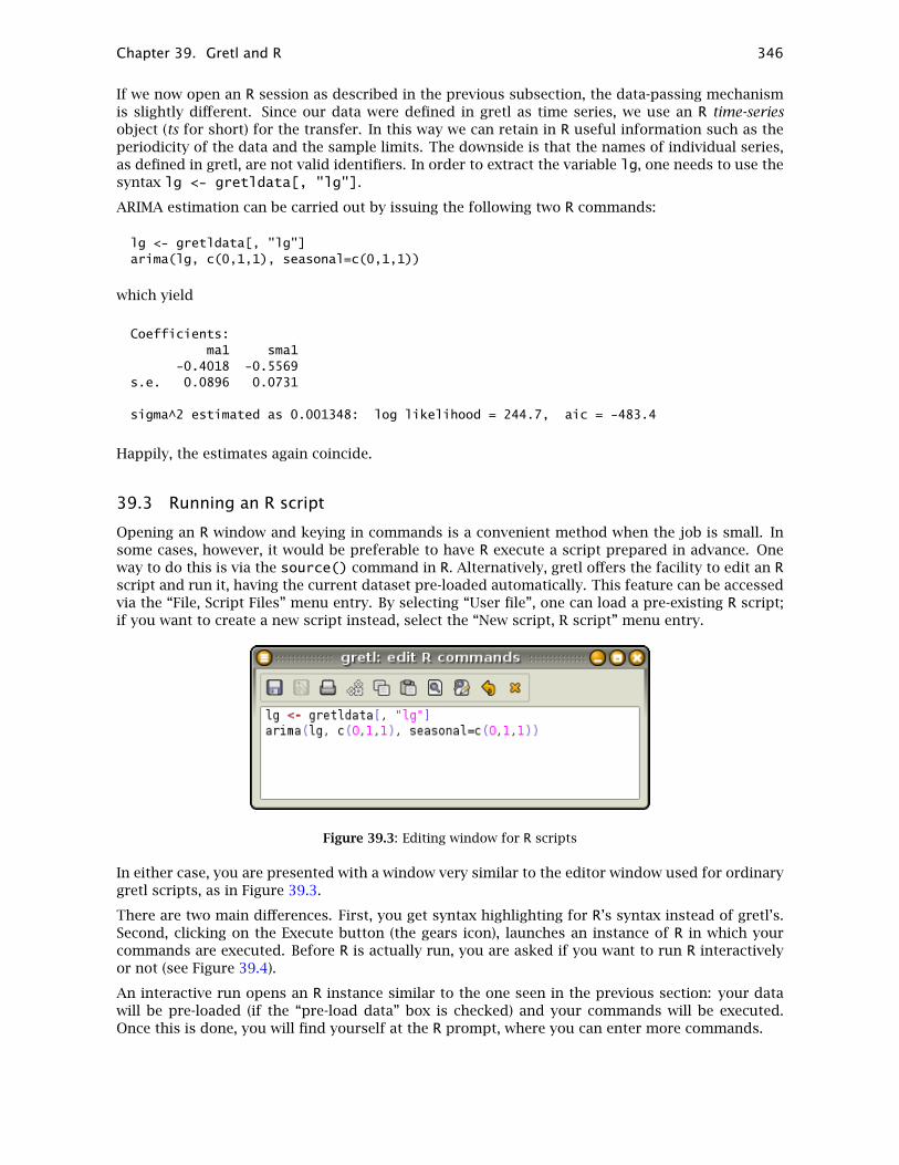
Chapter 39. Gretl and R 346
If we now open an R session as described in the previous subsection, the data-passing mechanismis slightly different. Since our data were defined in gretl as time series, we use an R time-seriesobject (ts for short) for the transfer. In this way we can retain in R useful information such as theperiodicity of the data and the sample limits. The downside is that the names of individual series,as defined in gretl, are not valid identifiers. In order to extract the variable lg, one needs to use thesyntax lg <- gretldata[, "lg"].
ARIMA estimation can be carried out by issuing the following two R commands:
lg <- gretldata[, "lg"]arima(lg, c(0,1,1), seasonal=c(0,1,1))
which yield
Coefficients:ma1 sma1
-0.4018 -0.5569s.e. 0.0896 0.0731
sigma^2 estimated as 0.001348: log likelihood = 244.7, aic = -483.4
Happily, the estimates again coincide.
39.3 Running an R script
Opening an R window and keying in commands is a convenient method when the job is small. Insome cases, however, it would be preferable to have R execute a script prepared in advance. Oneway to do this is via the source() command in R. Alternatively, gretl offers the facility to edit an Rscript and run it, having the current dataset pre-loaded automatically. This feature can be accessedvia the “File, Script Files” menu entry. By selecting “User file”, one can load a pre-existing R script;if you want to create a new script instead, select the “New script, R script” menu entry.
Figure 39.3: Editing window for R scripts
In either case, you are presented with a window very similar to the editor window used for ordinarygretl scripts, as in Figure 39.3.
There are two main differences. First, you get syntax highlighting for R’s syntax instead of gretl’s.Second, clicking on the Execute button (the gears icon), launches an instance of R in which yourcommands are executed. Before R is actually run, you are asked if you want to run R interactivelyor not (see Figure 39.4).
An interactive run opens an R instance similar to the one seen in the previous section: your datawill be pre-loaded (if the “pre-load data” box is checked) and your commands will be executed.Once this is done, you will find yourself at the R prompt, where you can enter more commands.

Chapter 39. Gretl and R 347
Figure 39.4: Editing window for R scripts
A non-interactive run, on the other hand, will execute your script, collect the output from R andpresent it to you in an output window; R will be run in the background. If, for example, the scriptin Figure 39.3 is run non-interactively, a window similar to Figure 39.5 will appear.
Figure 39.5: Output from a non-interactive R run
39.4 Taking stuff back and forth
As regards the passing of data between the two programs, so far we have only considered passingseries from gretl to R. In order to achieve a satisfactory degree of interoperability, more is needed.In the following sub-sections we see how matrices can be exchanged, and how data can be passedfrom R back to gretl.
Chapter 39. Gretl and R 348
Passing matrices from gretl to R
For passing matrices from gretl to R, you can use the mwrite matrix function described in section16.7. For example, the following gretl code fragment generates the matrix
A =
3 7 11
4 8 12
5 9 13
6 10 14
and stores it into the file mymatfile.mat.
matrix A = mshape(seq(3,14),4,3)err = mwrite(A, "mymatfile.mat")
The R code to import such a matrix is
A <- as.matrix(read.table("mymatfile.mat", skip=1))
Although in principle you can give your matrix file any valid filename, a couple of conventionsmay prove useful. First, you may want to use an informative file suffix such as “.mat”, but thisis a matter of taste. More importantly, the exact location of the file created by mwrite could bean issue. By default, if no path is specified in the file name, gretl writes matrix files in the currentworking directory. However, it may be wise for the purpose at hand to use a directory that is knownto be writable by the user, namely the user’s “dotdir”(see section 14.2). This can be achieved on thegretl side by passing a non-zero integer as the (optional) third argument to mwrite; on the R sideyou can use the function gretl.loadmat, which is pre-defined when R is called from gretl.4 So theabove example may be rewritten as
Gretl side:
mwrite(A, "mymatfile.mat", 1)
R side:
A <- gretl.loadmat("mymatfile.mat")
Passing data from R to gretl
For passing data in the opposite direction, gretl defines a special function that can be used in the Renvironment. An R object will be written as a temporary file in gretl’s dotdir directory, from whereit can be easily retrieved from within gretl.
The name of this function is gretl.export(); it takes one required argument, the object to beexported. At present, the objects that can be exported with this method are matrices, data framesand time-series objects. The function creates a text file, by default with the same name as theexported object (plus an appropriate suffix), in gretl’s temporary directory. Data frames and time-series objects are stored as CSV files, and can be retrieved by using gretl’s append command.Matrices are stored in a special text format that is understood by gretl (see section 16.7); the filesuffix is in this case .mat, and to read the matrix in gretl you must use the mread() function.
This function also has an optional second argument, namely a string which specifies a basenamefor the export file, in case you want to use a name other than that attached to the object within R.As in the default case an appropriate suffix, .csv or .mat, will be added to the basename.
4In case you need to do this sort of thing manually, you can use the built-in string variable dotdir in gretl, while in Ryou have the same variable under the name gretl.dotdir.
Chapter 39. Gretl and R 349
As an example, we take the airline data and use them to estimate a structural time series model àla Harvey (1989). The model we will use is the Basic Structural Model (BSM), in which a time seriesis decomposed into three terms:
yt = µt + γt + εtwhere µt is a trend component, γt is a seasonal component and εt is a noise term. In turn, thefollowing is assumed to hold:
∆µt = βt−1 + ηt∆βt = ζt∆sγt = ∆ωtwhere ∆s is the seasonal differencing operator, (1 − Ls), and ηt , ζt and ωt are mutually uncorre-lated white noise processes. The object of the analysis is to estimate the variances of the noisecomponents (which may be zero) and to recover estimates of the latent processes µt (the “level”),βt (the “slope”) and γt .
Gretl does not provide (yet) a command for estimating this class of models, so we will use R’sStructTS command and import the results back into gretl. Once the bjg dataset is loaded in gretl,we pass the data to R and execute the following script:
# extract the log seriesy <- gretldata[, "lg"]# estimate the modelstrmod <- StructTS(y)# save the fitted components (smoothed)compon <- as.ts(tsSmooth(strmod))# save the estimated variancesvars <- as.matrix(strmod$coef)
# export into gretl’s temp dirgretl.export(compon)gretl.export(vars)
Running this script via gretl produces minimal output:
current data loaded as ts object "gretldata"wrote /home/cottrell/.gretl/compon.csvwrote /home/cottrell/.gretl/vars.mat
However, we are now able to pull the results back into gretl by executing the following commands,either from the console or by creating a small script:
string fnamesprintf fname "%s/compon.csv", $dotdirappend @fnamevars = mread("vars.mat", 1)
The first command reads the estimated time-series components from a CSV file, which is the formatthat the passing mechanism employs for series. The matrix vars is read from the file vars.mat.
After the above commands have been executed, three new series will have appeared in the gretlworkspace, namely the estimates of the three components; by plotting them together with theoriginal data, you should get a graph similar to Figure 39.6. The estimates of the variances can beseen by printing the vars matrix, as in
? print varsvars (4 x 1)
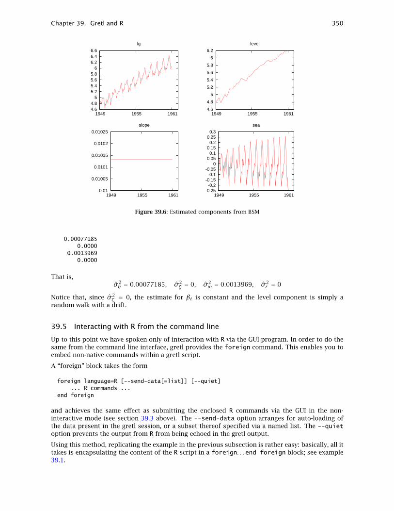
Chapter 39. Gretl and R 350
4.6 4.8
5 5.2 5.4 5.6 5.8
6 6.2 6.4 6.6
1949 1955 1961
lg
4.6
4.8
5
5.2
5.4
5.6
5.8
6
6.2
1949 1955 1961
level
0.01
0.01005
0.0101
0.01015
0.0102
0.01025
1949 1955 1961
slope
-0.25-0.2
-0.15-0.1
-0.05 0
0.05 0.1
0.15 0.2
0.25 0.3
1949 1955 1961
sea
Figure 39.6: Estimated components from BSM
0.000771850.0000
0.00139690.0000
That is,σ 2η = 0.00077185, σ 2
ζ = 0, σ 2ω = 0.0013969, σ 2
ε = 0
Notice that, since σ 2ζ = 0, the estimate for βt is constant and the level component is simply a
random walk with a drift.
39.5 Interacting with R from the command line
Up to this point we have spoken only of interaction with R via the GUI program. In order to do thesame from the command line interface, gretl provides the foreign command. This enables you toembed non-native commands within a gretl script.
A “foreign” block takes the form
foreign language=R [--send-data[=list]] [--quiet]... R commands ...
end foreign
and achieves the same effect as submitting the enclosed R commands via the GUI in the non-interactive mode (see section 39.3 above). The --send-data option arranges for auto-loading ofthe data present in the gretl session, or a subset thereof specified via a named list. The --quietoption prevents the output from R from being echoed in the gretl output.
Using this method, replicating the example in the previous subsection is rather easy: basically, all ittakes is encapsulating the content of the R script in a foreign. . . end foreign block; see example39.1.

Chapter 39. Gretl and R 351
Listing 39.1: Estimation of the Basic Structural Model – simple
open bjg.gdt
foreign language=R --send-datay <- gretldata[, "lg"]strmod <- StructTS(y)compon <- as.ts(tsSmooth(strmod))vars <- as.matrix(strmod$coef)
gretl.export(compon)gretl.export(vars)
end foreign
append @dotdir/compon.csvrename level lg_levelrename slope lg_sloperename sea lg_seas
vars = mread("vars.mat", 1)
Listing 39.2: Estimation of the Basic Structural Model – via a function
function list RStructTS(series myseries)
smpl ok(myseries) --restrictsx = argname(myseries)
foreign language=R --send-data --quiet@sx <- gretldata[, "myseries"]strmod <- StructTS(@sx)compon <- as.ts(tsSmooth(strmod))gretl.export(compon)
end foreign
append @dotdir/compon.csvrename level @sx_levelrename slope @sx_sloperename sea @sx_seas
list ret = @sx_level @sx_slope @sx_seasreturn ret
end function
# ------------ main -------------------------
open bjg.gdtlist X = RStructTS(lg)

Chapter 39. Gretl and R 352
The above syntax, despite being already quite useful by itself, shows its full power when it is usedin conjunction with user-written functions. Listing 39.2 shows how to define a gretl function thatcalls R internally.
39.6 Performance issues with R
R is a large and complex program, which takes an appreciable time to initialize itself.5 In interactiveuse this not a significant problem, but if you have a gretl script that calls R repeatedly the cumulatedstart-up costs can become bothersome. To get around this, gretl calls the R shared library bypreference; in this case the start-up cost is borne only once, on the first invocation of R code fromwithin gretl.
Support for the R shared library is built into the gretl packages for MS Windows and OS X—butthe advantage is realized only if the library is in fact available at run time. If you are building gretlyourself on Linux and wish to make use of the R library, you should ensure (a) that R has beenbuilt with the shared library enabled (specify --enable-R-shlib when configuring your build ofR), and (b) that the pkg-config program is able to detect your R installation. We do not link to theR library at build time, rather we open it dynamically on demand. The gretl GUI has an item underthe Tools/Preferences menu which enables you to select the path to the library, if it is not detectedautomatically.
If you have the R shared library installed but want to force gretl to call the R executable instead,you can do
set R_lib off
39.7 Further use of the R library
Besides improving performance, as noted above, use of the R shared library makes possible afurther refinement. That is, you can define functions in R, within a foreign block, then call thosefunctions later in your script much as if they were gretl functions. This is illustrated below.
set R_functions onforeign language=Rplus_one <- function(q)
z = q+1invisible(z)
end foreign
scalar b=R.plus_one(2)
The R function plus_one is obviously trivial in itself, but the example shows a couple of points.First, for this mechanism to work you need to enable R_functions via the set command. Second,to avoid collision with the gretl function namespace, calls to functions defined in this way must beprefixed with “R.”, as in R.plus_one.
Built-in R functions may also be called in this way, once R_functions is set on. For example onecan invoke R’s choose function, which computes binomial coefficients:
set R_functions onscalar b=R.choose(10,4)
Note, however, that the possibilities for use of built-in R functions are limited; only functions whosearguments and return values are sufficiently generic (basically scalars or matrices) will work.
5About one third of a second on an Intel Core Duo machine of 2009 vintage.

Chapter 40
Gretl and Ox
40.1 Introduction
Ox, written by Jurgen A. Doornik (see Doornik, 2007), is described by its author as “an object-oriented statistical system. At its core is a powerful matrix language, which is complemented bya comprehensive statistical library. Among the special features of Ox are its speed [and] well-designed syntax. . . . Ox comes in two versions: Ox Professional and Ox Console. Ox is available forWindows, Linux, Mac (OS X), and several Unix platforms.” (www.doornik.com)
Ox is proprietary, closed-source software. The command-line version of the program is, however,available free of change for academic users. Quoting again from Doornik’s website: “The Console(command line) versions may be used freely for academic research and teaching purposes only. . . .The Ox syntax is public, and, of course, you may do with your own Ox code whatever you wish.”If you wish to use Ox in conjunction with gretl please refer to doornik.com for further details onlicensing.
As the reader will no doubt have noticed, most other software that we discuss in this Guide is open-source and freely available for all users. We make an exception for Ox on the grounds that it isindeed fast and well designed, and that its statistical library—along with various add-on packagesthat are also available—has exceptional coverage of cutting-edge techniques in econometrics. Thegretl authors have used Ox for benchmarking some of gretl’s more advanced features such asdynamic panel models and state space models.1
40.2 Ox support in gretl
The support offered for Ox in gretl is similar to that offered for R, as discussed in chapter 39.
+ To enable support for Ox, go to the Tools/Preferences/General menu item and look under the Programstab. Find the entry for the path to the oxl executable, that is, the program that runs Ox files (on MS Windowsit is called oxl.exe). Adjust the path if it’s not already right for your system and you should be ready to go.
With support enabled, you can open and edit Ox programs in the gretl GUI. Clicking the “execute”icon in the editor window will send your code to Ox for execution. Figures 40.1 and Figure 40.2show an Ox program and part of its output.
In addition you can embed Ox code within a gretl script using a foreign block, as described inconnection with R. A trivial example, which simply prints the gretl data matrix within Ox, is shownbelow:
open data4-1matrix m = dataset mwrite(m, "gretl.mat", 1)
foreign language=Ox#include <oxstd.h>main()
1For a review of Ox, see Cribari-Neto and Zarkos (2003) and for a (somewhat dated) comparison of Ox with othermatrix-oriented packages such as GAUSS, see Steinhaus (1999).
353

Chapter 40. Gretl and Ox 354
Figure 40.1: Ox editing window
Figure 40.2: Output from Ox

Chapter 40. Gretl and Ox 355
decl gmat = gretl_loadmat("gretl.mat");print(gmat);
end foreign
The above example illustrates how a matrix can be passed from gretl to Ox. We use the mwritefunction to write a matrix into the user’s “dotdir” (see section 14.2), then in Ox we use the functiongretl_loadmat to retrieve the matrix.
How does gretl_loadmat come to be defined? When gretl writes out the Ox program correspond-ing to your foreign block it does two things in addition. First, it writes a small utility file namedgretl_io.ox into your dotdir. This contains a definition for gretl_loadmat and also for thefunction gretl_export (see below). Second, gretl interpolates into your Ox code a line which in-cludes this utility file (it is inserted right after the inclusion of oxstd.h, which is needed in all Oxprograms). Note that gretl_loadmat expects to find the named file in the user’s dotdir.
40.3 Illustration: replication of DPD model
Listing 40.1 shows a more ambitious case. This script replicates one of the dynamic panel datamodels in Arellano and Bond (1991), first using gretl and then using Ox; we then check the relativedifferences between the parameter estimates produced by the two programs (which turn out to bereassuringly small).
Unlike the previous example, in this case we pass the dataset from gretl to Ox as a CSV file inorder to preserve the variable names. Note the use of the internal variable csv_na to get the rightrepresentation of missing values for use with Ox—and also note that the --send-data option forthe foreign command is not available in connection with Ox.
We get the parameter estimates back from Ox using gretl_export on the Ox side and mread onthe gretl side. The gretl_export function takes two arguments, a matrix and a file name. The fileis written into the user’s dotdir, from where it can be picked up using mread. The final portion ofthe output from Listing 40.1 is shown below:
? matrix oxparm = mread("oxparm.mat", 1)Generated matrix oxparm? eval abs((parm - oxparm) ./ oxparm)1.4578e-133.5642e-135.0672e-151.6091e-138.9808e-152.0450e-141.0218e-132.1048e-139.5898e-151.8658e-142.1852e-142.9451e-131.9398e-13

Chapter 40. Gretl and Ox 356
Listing 40.1: Estimation of dynamic panel data model via gretl and Ox
open abdata.gdt
# Take first differences of the independent variablesgenr Dw = diff(w)genr Dk = diff(k)genr Dys = diff(ys)
# 1-step GMM estimationarbond 2 ; n Dw Dw(-1) Dk Dys Dys(-1) 0 --time-dummiesmatrix parm = $coeff
# Write CSV file for Oxset csv_na .NaNstore @dotdir/abdata.csv
# Replicate using the Ox DPD packageforeign language=Ox#include <oxstd.h>#import <packages/dpd/dpd>
main ()
decl dpd = new DPD();dpd.Load("@dotdir/abdata.csv");dpd.SetYear("YEAR");
dpd.Select(Y_VAR, "n", 0, 2);dpd.Select(X_VAR, "w", 0, 1, "k", 0, 0, "ys", 0, 1);dpd.Select(I_VAR, "w", 0, 1, "k", 0, 0, "ys", 0, 1);
dpd.Gmm("n", 2, 99); // GMM-type instrumentdpd.SetDummies(D_CONSTANT + D_TIME);dpd.SetTest(2, 2); // Sargan, AR 1-2 testsdpd.Estimate(); // 1-step estimationdecl parm = dpd.GetPar();gretl_export(parm, "oxparm.mat");
delete dpd;end foreign
# Compare the resultsmatrix oxparm = mread("oxparm.mat", 1)eval abs((parm - oxparm) ./ oxparm)

Chapter 41
Gretl and Octave
41.1 Introduction
GNU Octave, written by John W. Eaton and others, is described as “a high-level language, primar-ily intended for numerical computations.” The program is oriented towards “solving linear andnonlinear problems numerically” and “performing other numerical experiments using a languagethat is mostly compatible with Matlab.” (www.gnu.org/software/octave) Octave is available insource-code form (naturally, for GNU software) and also in the form of binary packages for MS Win-dows and Mac OS X. Numerous contributed packages that extend Octave’s functionality in variousways can be found at octave.sf.net.
41.2 Octave support in gretl
The support offered for Octave in gretl is similar to that offered for R (chapter 39). For example,you can open and edit Octave scripts in the gretl GUI. Clicking the “execute” icon in the editorwindow will send your code to Octave for execution. Figures 41.1 and Figure 41.2 show an Octavescript and its output; in this example we use the function logistic_regression to replicate someresults from Greene (2000).
In addition you can embed Octave code within a gretl script using a foreign block, as describedin connection with R. A trivial example, which simply loads and prints the gretl data matrix withinOctave, is shown below. (Note that in Octave, appending “;” to a line suppresses verbose output;leaving off the semicolon results in printing of the object that is produced, if any.)
open data4-1matrix m = dataset mwrite(m, "gretl.mat", 1)
foreign language=Octavegmat = gretl_loadmat("gretl.mat")
end foreign
We use the mwrite function to write a matrix into the user’s “dotdir” (see section 14.2), then in Oc-tave we use the function gretl_loadmat to retrieve the matrix. The “magic” behind gretl_loadmatworks in essentially the same way as for Ox (chapter 40).
41.3 Illustration: spectral methods
We now present a more ambitious example which exploits Octave’s handling of the frequencydomain (and also its ability to use code written for MATLAB), namely estimation of the spec-tral coherence of two time series. For this illustration we require two extra Octave packagesfrom octave.sf.net, namely those supporting spectral functions (specfun) and signal process-ing (signal). After downloading the packages you can install them from within Octave as follows(using version numbers as of March 2010):
pkg install specfun-1.0.8.tar.gzpkg install signal-1.0.10.tar.gz
357

Chapter 41. Gretl and Octave 358
Figure 41.1: Octave editing window
Figure 41.2: Output from Octave

Chapter 41. Gretl and Octave 359
In addition we need some specialized MATLAB files made available by Mario Forni of the Univer-sity of Modena, at http://morgana.unimore.it/forni_mario/matlab.htm. The files needed arecoheren2.m, coheren.m, coher.m, cospec.m, crosscov.m, crosspec.m, crosspe.m and spec.m.These are in a form appropriate for MS Windows. On Linux you could run the following shell scriptto get the files and remove the Windows end-of-file character (which prevents the files from runningunder Octave):
SITE=http://morgana.unimore.it/forni_mario/MYPROG# download files and delete trailing Ctrl-Zfor f in \coheren2.m \coheren.m \coher.m \cospec.m \crosscov.m \crosspec.m \crosspe.m \spec.m ; dowget $SITE/$f && \cat $f | tr -d \\032 > tmp.m && mv tmp.m $f
done
The Forni files should be placed in some appropriate directory, and you should tell Octave whereto find them by adding that directory to Octave’s loadpath. On Linux this can be done via an entryin one’s ~/.octaverc file. For example
addpath("~/stats/octave/forni");
Alternatively, an addpath directive can be written into the Octave script that calls on these files.
With everything set up on the Octave side we now write a gretl script (see Listing 41.1) which opensa time-series dataset, constructs and writes a matrix containing two series, and defines a foreignblock containing the Octave statements needed to produce the spectral coherence matrix. Thematrix is exported via the gretl_export function, which is automatically defined for you; thisfunction takes two arguments, a matrix and a file name. The file is written into the user’s “dotdir”,from where it can be picked up using mread. Finally, we produce a graph from the matrix in gretl.In the script this is sent to the screen; Figure 41.3 shows the same graph in PDF format.

Chapter 41. Gretl and Octave 360
Listing 41.1: Estimation of spectral coherence via Octave
open data9-7matrix xy = PRIME, UNEMP mwrite(xy, "xy.mat", 1)
foreign language=Octave# uncomment and modify the following if necessary# addpath("~/stats/octave/forni");xy = gretl_loadmat("xy.mat");x = xy(:,1);y = xy(:,2);# note: the last parameter is the Bartlett window sizeh = coher(x, y, 8);gretl_export(h, "h.mat");
end foreign
h = mread("h.mat", 1)colnames(h, "coherence")gnuplot 1 --time-series --with-lines --matrix=h --output=display
-0.5
-0.4
-0.3
-0.2
-0.1
0
0.1
0.2
0.3
0.4
0 10 20 30 40 50 60
cohere
nce
Figure 41.3: Spectral coherence estimated via Octave

Chapter 42
Gretl and Stata
Stata (www.stata.com) is closed-source, proprietary (and expensive) software and as such is not anatural companion to gretl. Nonetheless, given Stata’s popularity it is desirable to have a convenientway of comparing results across the two programs, and to that end we provide some support forStata code under the foreign command.
+ To enable support for Stata, go to the Tools/Preferences/General menu item and look under the Programstab. Find the entry for the path to the Stata executable. Adjust the path if it’s not already right for yoursystem and you should be ready to go.
The following example illustrates what’s available. You can send the current gretl dataset to Statausing the --send-data flag. And having defined a matrix within Stata you can export it for use withgretl via the gretl_export command: this takes two arguments, the name of the matrix to exportand the filename to use; the file is written to the user’s “dotdir”, from where it can be retrievedusing the mread() function.1 To suppress printed output from Stata you can add the --quiet flagto the foreign block.
Listing 42.1: Comparison of clustered standard errors with Stata
function matrix stata_reorder (matrix se)# stata puts the intercept last, but gretl puts it firstscalar n = rows(se)return se[n] | se[1:n-1]
end function
open data4-1ols 1 0 2 3 --cluster=bedrmsmatrix se = $stderr
foreign language=stata --send-dataregress price sqft bedrms, vce(cluster bedrms)matrix vcv = e(V)gretl_export vcv "vcv.mat"
end foreign
matrix stata_vcv = mread("vcv.mat", 1)stata_se = stata_reorder(sqrt(diag(stata_vcv)))matrix check = se - stata_seprint check
In addition you can edit “pure” Stata scripts in the gretl GUI and send them for execution as withnative gretl scripts.
Note that Stata coerces all variable names to lower-case on data input, so even if series names in
1We do not currently offer the complementary functionality of gretl_loadmat, which enables reading of matriceswritten by gretl’s mwrite() function in Ox and Octave. This is not at all easy to implement in Stata code.
361

Chapter 42. Gretl and Stata 362
gretl are upper-case, or of mixed case, it’s necessary to use all lower-case in Stata. Also note thatwhen opening a data file within Stata via the use command it will be necessary to provide the fullpath to the file.

Chapter 43
Gretl and Python
43.1 Introduction
According to www.python.org, Python is “an easy to learn, powerful programming language. It hasefficient high-level data structures and a simple but effective approach to object-oriented program-ming. Python’s elegant syntax and dynamic typing, together with its interpreted nature, make it anideal language for scripting and rapid application development in many areas on most platforms.”
Indeed, Python is widely used in a great variety of contexts. Numerous add-on modules are avail-able; the ones likely to be of greatest interest to econometricians include NumPy (“the fundamen-tal package for scientific computing with Python”—see www.numpy.org); SciPy (which builds onNumPy—see www.scipy.org); and Statsmodels (http://statsmodels.sourceforge.net/).
43.2 Python support in gretl
The support offered for Python in gretl is similar to that offered for Octave (chapter 41). You canopen and edit Python scripts in the gretl GUI. Clicking the “execute” icon in the editor window willsend your code to Python for execution. In addition you can embed Python code within a gretlscript using a foreign block, as described in connection with R.
When you launch Python from within gretl one variable and two convenience functions are pre-defined, as follows.
gretl_dotdirgretl_loadmat(filename, autodot=1)gretl_export(M, filename, autodot=1)
The variable gretl_dotdir holds the path to the user’s “dot directory.” The first function loads amatrix of the given filename as written by gretl’s mwrite function, and the second writes matrixM, under the given filename, in the format wanted by gretl.
By default the traffic in matrices goes via the dot directory on the Python side; that is, the name ofthis directory is prepended to filename for both reading and writing. (This is complementary touse of the export and import parameters with gretl’s mwrite and mread functions, respectively.)However, if you wish to take control over the reading and writing locations you can supply a zerovalue for autodot when calling gretl_loadmat and gretl_export: in that case the filenameargument is used as is.
Note that gretl_loadmat and gretl_export depend on NumPy; they make use of the functionsloadtxt and savetxt respectively. Nonetheless, the presence of NumPy is not an absolute require-ment if you don’t need to use these two functions.
43.3 Illustration: linear regression with multicollinearity
Listing 43.1 compares the numerical accuracy of gretl’s ols command with that of NumPy’s linalg.lstsq,using the notorious Longley test data which exhibit extreme multicollinearity. Unlike some econo-metrics packages, NumPy does a good job on these data. The script computes and prints thelog-relative error in estimation of the regression coefficients, using the NIST-certified values as a
363

Chapter 43. Gretl and Python 364
benchmark;1 the error values correspond to the number of correct digits (with a maximum of 15).The results will differ somewhat by computer architecture; the output shown was obtained on a32-bit Linux Intel i5 system.
1See http://www.itl.nist.gov/div898/strd/lls/data/Longley.shtml.

Chapter 43. Gretl and Python 365
Listing 43.1: Comparing regression results with Python
set echo offset messages off
function matrix logrel_error (matrix est, matrix true)return -log10(abs(est - true) ./ abs(true))
end function
open longley.gdt -qlist LX = prdefl .. year# gretl’s regular OLSols employ 0 LX -qmatrix b = $coeff
mwrite(employ, "y.mat", 1)mwrite(const ~ LX, "X.mat", 1)
foreign language=pythonimport numpy as npy = gretl_loadmat(’y.mat’, 1)X = gretl_loadmat(’X.mat’, 1)# NumPy’s OLSb = np.linalg.lstsq(X, y)[0]gretl_export(np.transpose(np.matrix(b)), ’py_b.mat’, 1)
end foreign
# NIST’s certified coefficient valuesmatrix nist_b = -3482258.63459582, 15.0618722713733,
-0.358191792925910E-01, -2.02022980381683,-1.03322686717359, -0.511041056535807E-01,1829.15146461355’
matrix py_b = mread("py_b.mat", 1)matrix errs = logrel_error(b, nist_b) ~ logrel_error(py_b, nist_b)colnames(errs, "gretl python")printf "Log-relative errors, Longley coefficients:\n\n%12.5g\n", errsprintf "Column means\n%12.5g\n", meanc(errs)
Output:
Log-relative errors, Longley coefficients:
gretl python12.844 12.8511.528 11.41412.393 12.40113.135 13.12113.738 13.31812.587 12.36312.848 12.852
Column means12.725 12.617

Chapter 44
Gretl and Julia
44.1 Introduction
According to julialang.org, Julia is “a high-level, high-performance dynamic programming lan-guage for technical computing, with syntax that is familiar to users of other technical computingenvironments. It provides a sophisticated compiler, distributed parallel execution, numerical accu-racy, and an extensive mathematical function library.” Julia is well known for being very fast.
44.2 Julia support in gretl
The support offered for Julia in gretl is similar to that offered for Octave (chapter 41). You canopen and edit Julia scripts in the gretl GUI. Clicking the “execute” icon in the editor window willsend your code to Julia for execution. In addition you can embed Julia code within a gretl scriptusing a foreign block, as described in connection with R.
When you launch Julia from within gretl one variable and two convenience functions are pre-defined,as follows.
gretl_dotdirgretl_loadmat(filename, autodot=true)gretl_export(M, filename, autodot=true)
The variable gretl_dotdir holds the path to the user’s “dot directory.” The first function loads amatrix of the given filename as written by gretl’s mwrite function, and the second writes matrixM, under the given filename, in the format wanted by gretl.
By default the traffic in matrices goes via the dot directory on the Julia side; that is, the name ofthis directory is prepended to filename for both reading and writing. (This is complementary touse of the export and import parameters with gretl’s mwrite and mread functions, respectively.)However, if you wish to take control over the reading and writing locations you can supply a zerovalue for autodot when calling gretl_loadmat and gretl_export: in that case the filenameargument is used as is.
44.3 Illustration
TO BE WRITTEN!
366

Chapter 45
Troubleshooting gretl
45.1 Bug reports
Bug reports are welcome—well, if not exactly welcome then useful and appreciated. Hopefully, youare unlikely to find bugs in the actual calculations done by gretl (although this statement does notconstitute any sort of warranty). You may, however, come across bugs or oddities in the behaviorof the graphical interface. Please remember that the usefulness of bug reports is greatly enhancedif you can be as specific as possible: what exactly went wrong, under what conditions, and on whatoperating system? If you saw an error message, what precisely did it say?
One way of making a bug report more useful is to run the program in such a way that you can see(and copy) any additional information that gets printed to the stderr output stream. On Linux andMac OS X that’s just a matter of launching gretl from the command prompt in a terminal window.On MS Windows it’s a bit more complicated since stderr is by default “invisble.” However, you canquite easily set up a special gretl shortcut that does the job. On the Windows desktop, right-clickand select “New shortcut.” In the dialog box that appears, browse to find gretl.exe and appendthe --debug flag, as shown in Figure 45.1. Note that there are two dashes before “debug”.
Figure 45.1: Creating a debugging shortcut
367
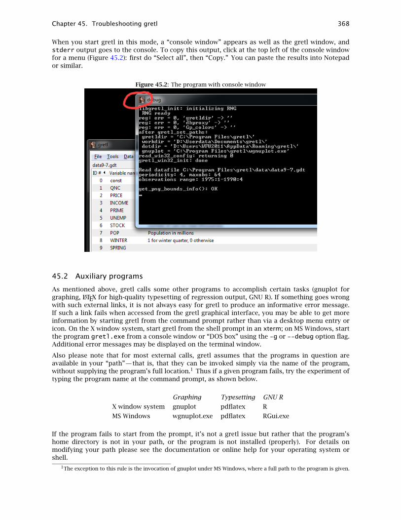
Chapter 45. Troubleshooting gretl 368
When you start gretl in this mode, a “console window” appears as well as the gretl window, andstderr output goes to the console. To copy this output, click at the top left of the console windowfor a menu (Figure 45.2): first do “Select all”, then “Copy.” You can paste the results into Notepador similar.
Figure 45.2: The program with console window
45.2 Auxiliary programs
As mentioned above, gretl calls some other programs to accomplish certain tasks (gnuplot forgraphing, LATEX for high-quality typesetting of regression output, GNU R). If something goes wrongwith such external links, it is not always easy for gretl to produce an informative error message.If such a link fails when accessed from the gretl graphical interface, you may be able to get moreinformation by starting gretl from the command prompt rather than via a desktop menu entry oricon. On the X window system, start gretl from the shell prompt in an xterm; on MS Windows, startthe program gretl.exe from a console window or “DOS box” using the -g or --debug option flag.Additional error messages may be displayed on the terminal window.
Also please note that for most external calls, gretl assumes that the programs in question areavailable in your “path”—that is, that they can be invoked simply via the name of the program,without supplying the program’s full location.1 Thus if a given program fails, try the experiment oftyping the program name at the command prompt, as shown below.
Graphing Typesetting GNU R
X window system gnuplot pdflatex R
MS Windows wgnuplot.exe pdflatex RGui.exe
If the program fails to start from the prompt, it’s not a gretl issue but rather that the program’shome directory is not in your path, or the program is not installed (properly). For details onmodifying your path please see the documentation or online help for your operating system orshell.
1The exception to this rule is the invocation of gnuplot under MS Windows, where a full path to the program is given.

Chapter 46
The command line interface
The gretl package includes the command-line program gretlcli. On Linux it can be run from aterminal window (xterm, rxvt, or similar), or at the text console. Under MS Windows it can be run ina console window (sometimes inaccurately called a “DOS box”). gretlcli has its own help file, whichmay be accessed by typing “help” at the prompt. It can be run in batch mode, sending outputdirectly to a file (see also the Gretl Command Reference).
If gretlcli is linked to the readline library (this is automatically the case in the MS Windows version;also see Appendix C), the command line is recallable and editable, and offers command completion.You can use the Up and Down arrow keys to cycle through previously typed commands. On a givencommand line, you can use the arrow keys to move around, in conjunction with Emacs editingkeystrokes.1 The most common of these are:
Keystroke Effect
Ctrl-a go to start of line
Ctrl-e go to end of line
Ctrl-d delete character to right
where “Ctrl-a” means press the “a” key while the “Ctrl” key is also depressed. Thus if you wantto change something at the beginning of a command, you don’t have to backspace over the wholeline, erasing as you go. Just hop to the start and add or delete characters. If you type the firstletters of a command name then press the Tab key, readline will attempt to complete the commandname for you. If there’s a unique completion it will be put in place automatically. If there’s morethan one completion, pressing Tab a second time brings up a list.
Probably the most useful mode for heavy-duty work with gretlcli is batch (non-interactive) mode,in which the program reads and processes a script, and sends the output to file. For example
gretlcli -b scriptfile > outputfile
Note that scriptfile is treated as a program argument; only the output file requires redirection (>).Don’t forget the -b (batch) switch, otherwise the program will wait for user input after executingthe script (and if output is redirected, the program will appear to “hang”).
1Actually, the key bindings shown below are only the defaults; they can be customized. See the readline manual.
369

Part IV
Appendices
370

Appendix A
Data file details
A.1 Basic native format
In gretl’s basic native data format–for which we use the suffix gdt—a data set is stored in XML(extensible mark-up language). Data files correspond to the simple DTD (document type defini-tion) given in gretldata.dtd, which is supplied with the gretl distribution and is installed in thesystem data directory (e.g. /usr/share/gretl/data on Linux.) Such files may be plain text (un-compressed) or gzipped. They contain the actual data values plus additional information such asthe names and descriptions of variables, the frequency of the data, and so on.
In a gdt file the actual data values are written to 17 significant figures (for generated data such aslogs or pseudo-random numbers) or to a maximum of 15 figures for primary data. The C printfformat “%.*g” is used (for * = 17 or 15) so that trailing zeros are not printed.
Most users will probably not have need to read or write such files other than via gretl itself, butif you want to manipulate them using other software tools you should examine the DTD and alsotake a look at a few of the supplied practice data files: data4-1.gdt gives a simple example;data4-10.gdt is an example where observation labels are included.
A.2 Binary data file format
As of gretl 1.9.15, an alternative, binary format is available for data storage. Files of this sort havesuffix gdtb, and they take the form of a PKZIP archive containing two files, data.xml and data.bin,with the following characteristics.
• data.xml is an XML file conforming to the gretldata DTD mentioned above, holding all themetadata.
• data.bin starts with a header composed of one of the strings
gretl-bin:little-endian orgretl-bin:big-endian
padded to 24 bytes with nul characters. This is followed by a binary dump of the data series,by variable, as double-precision floating-point values.
Binary values are saved in the endianness of the machine on which they’re written; the headerinformation enables gretl to convert to the endianness of the host on which the data are read ifneed be.
The rationale for introducing the binary gdtb format is that for very large datasets it is a lot fasterto write and read data in this form rather than as text. For small to moderately sized datasets(say, up to 10 megabytes or so) there is no appreciable advantage in the binary format and werecommend use of plain gdt.
Some illustrative timings are shown in Table A.1; these were obtained on a Lenovo ThinkPad X1 Car-bon running gretl 1.9.15. The datasets contained a mixture of random normal series and randombinary (dummy) series. The largest comprised 50000 observations on 1000 series and the smallest5000 observations on 250 series. As can be seen, there is a big time saving from the binary for-mat when writing (and to a lesser extent, when reading) a dataset in the hundreds of megabytes
371

Appendix A. Data file details 372
range. At a size of around 10 megabytes, however, gdt files can be both written and read in undera second, surely fast enough for most purposes.
381 MB 38 MB 19 MB 10 MB
format write read write read write read write read
gdt 21.76 4.91 2.20 0.48 1.19 0.32 0.59 0.16
gdtb 3.82 1.10 0.39 0.11 0.25 0.06 0.13 0.03
Table A.1: Data write and read timings in seconds for datasets of various sizes in megabytes. The MBnumbers represent the size of the datasets in memory; files of both formats are substantially smaller whencompression is applied.
A.3 Native database format
A gretl database consists of two parts: an ASCII index file (with filename suffix .idx) containinginformation on the series, and a binary file (suffix .bin) containing the actual data. Two examplesof the format for an entry in the idx file are shown below:
G0M910 Composite index of 11 leading indicators (1987=100)M 1948.01 - 1995.11 n = 575currbal Balance of Payments: Balance on Current Account; SAQ 1960.1 - 1999.4 n = 160
The first field is the series name. The second is a description of the series (maximum 128 charac-ters). On the second line the first field is a frequency code: M for monthly, Q for quarterly, A forannual, B for business-daily (daily with five days per week) and D for daily (seven days per week).No other frequencies are accepted at present. Then comes the starting date (N.B. with two digitsfollowing the point for monthly data, one for quarterly data, none for annual), a space, a hyphen,another space, the ending date, the string “n = ” and the integer number of observations. In thecase of daily data the starting and ending dates should be given in the form YYYY/MM/DD. Thisformat must be respected exactly.
Optionally, the first line of the index file may contain a short comment (up to 64 characters) on thesource and nature of the data, following a hash mark. For example:
# Federal Reserve Board (interest rates)
The corresponding binary database file holds the data values, represented as “floats”, that is, single-precision floating-point numbers, typically taking four bytes apiece. The numbers are packed “byvariable”, so that the first n numbers are the observations of variable 1, the next m the observationson variable 2, and so on.

Appendix B
Data import via ODBC
Since version 1.7.5, gretl provides a method for retrieving data from databases which support theOpen Database Connectivity (ODBC) standard. Most users won’t be interested in this, but there maybe some for whom this feature matters a lot — typically, those who work in an environment wherehuge data collections are accessible via a Data Base Management System (DBMS).
In the following section we explain what is needed for ODBC support in gretl. We provide somebackground information on how ODBC works in section B.2, and explain the details of getting gretlto retrieve data from a database in section B.3.
B.1 ODBC support
The piece of software that bridges between gretl and the ODBC system is a dynamically loaded“plugin”. This is included in the gretl packages for MS Windows and Mac OS X (on OS X supportwas added in gretl 1.9.0). On other unix-type platforms (notably Linux) you will have to build gretlfrom source to get ODBC support. This is because the gretl plugin depends on having unixODBCinstalled, which we cannot assume to be the case on typical Linux systems. To enable the ODBCplugin when building gretl, you must pass the option --with-odbc to gretl’s configure script. Inaddition, if unixODBC is installed in a non-standard location you will have to specify its installationprefix using --with-ODBC-prefix, as in (for example)
./configure --with-odbc --with-ODBC-prefix=/opt/ODBC
B.2 ODBC base concepts
ODBC is short for Open DataBase Connectivity, a group of software methods that enable a client tointeract with a database server. The most common operation is when the client fetches some datafrom the server. ODBC acts as an intermediate layer between client and server, so the client “talks”to ODBC rather than accessing the server directly (see Figure B.1).
ODBC
query
data
Figure B.1: Retrieving data via ODBC
For the above mechanism to work, it is necessary that the relevant ODBC software is installedand working on the client machine (contact your DB administrator for details). At this point, thedatabase (or databases) that the server provides will be accessible to the client as a data sourcewith a specific identifier (a Data Source Name or DSN); in most cases, a username and a passwordare required to connect to the data source.
Once the connection is established, the user sends a query to ODBC, which contacts the databasemanager, collects the results and sends them back to the user. The query is almost invariably
373

Appendix B. Data import via ODBC 374
formulated in a special language used for the purpose, namely SQL.1 We will not provide here anSQL tutorial: there are many such tutorials on the Net; besides, each database manager tends tosupport its own SQL dialect so the precise form of an SQL query may vary slightly if the DBMS onthe other end is Oracle, MySQL, PostgreSQL or something else.
Suffice it to say that the main statement for retrieving data is the SELECT statement. Within a DBMS,data are organized in tables, which are roughly equivalent to spreadsheets. The SELECT statementreturns a subset of a table, which is itself a table. For example, imagine that the database holds atable called “NatAccounts”, containing the data shown in Table B.1.
year qtr gdp consump tradebal
1970 1 584763 344746.9 −5891.01
1970 2 597746 350176.9 −7068.71
1970 3 604270 355249.7 −8379.27
1970 4 609706 361794.7 −7917.61
1971 1 609597 362490 −6274.3
1971 2 617002 368313.6 −6658.76
1971 3 625536 372605 −4795.89
1971 4 630047 377033.9 −6498.13
Table B.1: The “NatAccounts” table
The SQL statement
SELECT qtr, tradebal, gdp FROM NatAccounts WHERE year=1970;
produces the subset of the original data shown in Table B.2.
qtr tradebal gdp
1 −5891.01 584763
2 −7068.71 597746
3 −8379.27 604270
4 −7917.61 609706
Table B.2: Result of a SELECT statement
Gretl provides a mechanism for forwarding your query to the DBMS via ODBC and including theresults in your currently open dataset.
B.3 Syntax
At present gretl does not offer a graphical interface for ODBC import; this must be done via thecommand line interface. The two commands used for fetching data via an ODBC connection areopen and data.
The open command is used for connecting to a DBMS: its syntax is
open dsn=database [user=username] [password=password] --odbc
The user and password items are optional; the effect of this command is to initiate an ODBCconnection. It is assumed that the machine gretl runs on has a working ODBC client installed.
In order to actually retrieve the data, the data command is used. Its syntax is:
1See http://en.wikipedia.org/wiki/SQL.

Appendix B. Data import via ODBC 375
data series [obs-format=format-string] query=query-string --odbc
where:
series is a list of names of gretl series to contain the incoming data, separated by spaces. Note thatthese series need not exist pior to the ODBC import.
format-string is an optional parameter, used to handle cases when a “rectangular” organisation ofthe database cannot be assumed (more on this later);
query-string is a string containing the SQL statement used to extract the data.2
There should be no spaces around the equals signs in the obs-format and query fields in the datacommand.
The query-string can, in principle, contain any valid SQL statement which results in a table. Thisstring may be specified directly within the command, as in
data x query="SELECT foo FROM bar" --odbc
which will store into the gretl variable x the content of the column foo from the table bar. However,since in a real-life situation the string containing the SQL statement may be rather long, it may bebest to store it in a string variable. For example:
string SqlQry = "SELECT foo1, foo2 FROM bar"data x y query=SqlQry --odbc
The observation format specifier
If the optional parameter obs-format is absent, as in the above example, the SQL query shouldreturn k columns of data, where k is the number of series names listed in the data command.It may be necessary to include a smpl command before the data command to set up the right“window” for the incoming data. In addition, if one cannot assume that the data will be deliveredin the correct order (typically, chronological order), the SQL query should contain an appropriateORDER BY clause.
The optional format string is used for those cases when there is no certainty that the data from thequery will arrive in the same order as the gretl dataset. This may happen when missing values areinterspersed within a column, or with data that do not have a natural ordering, e.g. cross-sectionaldata. In this case, the SQL statement should return a table with m + k columns, where the first mcolumns are used to identify the observation or row in the gretl dataset into which the actual datavalues in the final k columns should be placed. The obs-format string is used to translate the firstm fields into a string which matches the string gretl uses to identify observations in the currentlyopen dataset. Up to three columns can be used for this purpose (m ≤ 3).
Note that the strings gretl uses to identify observations can be seen by printing any variable “byobservation”, as in
print index --byobs
(The series named index is automatically added to a dataset created via the nulldata command.)
The format specifiers available for use with obs-format are as follows:
%d print an integer value
%s print an string value
%g print a floating-point value
2Prior to gretl 1.8.8, the tag “query=” was not required (or accepted) before the query string, and only one seriescould be imported at a time. This variant is still accepted for the sake of backward compatibility.

Appendix B. Data import via ODBC 376
In addition the format can include literal characters to be passed through, such as slashes or colons,to make the resulting string compatible with gretl’s observation identifiers.
For example, consider the following fictitious case: we have a 5-days-per-week dataset, to which wewant to add the stock index for the Verdurian market;3 it so happens that in Verduria Saturdaysare working days but Wednesdays are not. We want a column which does not contain data onSaturdays, because we wouldn’t know where to put them, but at the same time we want to placemissing values on all the Wednesdays.
In this case, the following syntax could be used
string QRY="SELECT year,month,day,VerdSE FROM AlmeaIndexes"data y obs-format="%d/%d/%d" query=QRY --odbc
The column VerdSE holds the data to be fetched, which will go into the gretl series y. The firstthree columns are used to construct a string which identifies the day. Daily dates take the formYYYY/MM/DD in gretl. If a row from the DBMS produces the observation string 2008/04/01 this willmatch OK (it’s a Tuesday), but 2008/04/05 will not match since it is a Saturday; the correspondingrow will therefore be discarded. On the other hand, since no string 2008/04/23 will be found inthe data coming from the DBMS (it’s a Wednesday), that entry is left blank in our series y.
B.4 Examples
Table Consump Table DATA
Field Type
time decimal(7,2)
income decimal(16,6)
consump decimal(16,6)
Field Type
year decimal(4,0)
qtr decimal(1,0)
varname varchar(16)
xval decimal(20,10)
Table B.3: Example AWM database – structure
Table Consump Table DATA
1970.00 424278.975500 344746.944000
1970.25 433218.709400 350176.890400
1970.50 440954.219100 355249.672300
1970.75 446278.664700 361794.719900
1971.00 447752.681800 362489.970500
1971.25 453553.860100 368313.558500
1971.50 460115.133100 372605.015300
. . .
1970 1 CAN −517.9085000000
1970 2 CAN 662.5996000000
1970 3 CAN 1130.4155000000
1970 4 CAN 467.2508000000
1970 1 COMPR 18.4000000000
1970 2 COMPR 18.6341000000
1970 3 COMPR 18.3000000000
1970 4 COMPR 18.2663000000
1970 1 D1 1.0000000000
1970 2 D1 0.0000000000
. . .
Table B.4: Example AWM database — data
In the following examples, we will assume that access is available to a database known to ODBCwith the data source name “AWM”, with username “Otto” and password “Bingo”. The database“AWM” contains quarterly data in two tables (see B.3 and B.4):
3See http://www.almeopedia.com/index.php/Verduria.
Appendix B. Data import via ODBC 377
The table Consump is the classic “rectangular” dataset; that is, its internal organization is the sameas in a spreadsheet or econometrics package: each row is a data point and each column is a variable.The structure of the DATA table is different: each record is one figure, stored in the column xval,and the other fields keep track of which variable it belongs to, for which date.
Listing B.1: Simple query from a rectangular table
nulldata 160setobs 4 1970:1 --timeopen dsn=AWM user=Otto password=Bingo --odbc
string Qry = "SELECT consump, income FROM Consump"data cons inc query=Qry --odbc
Listing B.1 shows a query for two series: first we set up an empty quarterly dataset. Then weconnect to the database using the open statement. Once the connection is established we retrievetwo columns from the Consump table. No observation string is required because the data alreadyhave a suitable structure; we need only import the relevant columns.
Listing B.2: Simple query from a non-rectangular table
string S = "select year, qtr, xval from DATA \where varname=’WLN’ ORDER BY year, qtr"
data wln obs-format="%d:%d" query=S --odbc
In example B.2, by contrast, we make use of the observation string since we are drawing from theDATA table, which is not rectangular. The SQL statement stored in the string S produces a table withthree columns. The ORDER BY clause ensures that the rows will be in chronological order, althoughthis is not strictly necessary in this case.

Appendix B. Data import via ODBC 378
Listing B.3: Handling of missing values for a non-rectangular table
string foo = "select year, qtr, xval from DATA \where varname=’STN’ AND qtr>1"
data bar obs-format="%d:%d" query=foo --odbcprint bar --byobs
Listing B.3 shows what happens if the rows in the outcome from the SELECT statement do notmatch the observations in the currently open gretl dataset. The query includes a condition whichfilters out all the data from the first quarter. The query result (invisible to the user) would besomething like
+------+------+---------------+| year | qtr | xval |+------+------+---------------+| 1970 | 2 | 7.8705000000 || 1970 | 3 | 7.5600000000 || 1970 | 4 | 7.1892000000 || 1971 | 2 | 5.8679000000 || 1971 | 3 | 6.2442000000 || 1971 | 4 | 5.9811000000 || 1972 | 2 | 4.6883000000 || 1972 | 3 | 4.6302000000 |...
Internally, gretl fills the variable bar with the corresponding value if it finds a match; otherwise, NAis used. Printing out the variable bar thus produces
Obs bar
1970:11970:2 7.87051970:3 7.56001970:4 7.18921971:11971:2 5.86791971:3 6.24421971:4 5.98111972:11972:2 4.68831972:3 4.6302
...

Appendix C
Building gretl
Here we give instructions detailed enough to allow a user with only a basic knowledge of a Unix-type system to build gretl. These steps were tested on a fresh installation of Debian Etch. For otherLinux distributions (especially Debian-based ones, like Ubuntu and its derivatives) little shouldchange. Other Unix-like operating systems such as Mac OS X and BSD would probably require moresubstantial adjustments.
In this guided example, we will build gretl complete with documentation. This introduces a fewmore requirements, but gives you the ability to modify the documentation files as well, like thehelp files or the manuals.
C.1 Installing the prerequisites
We assume that the basic GNU utilities are already installed on the system, together with theseother programs:
• some TEX/LATEXsystem (texlive will do beautifully)
• Gnuplot
• ImageMagick
We also assume that the user has administrative privileges and knows how to install packages. Theexamples below are carried out using the apt-get shell command, but they can be performed withmenu-based utilities like aptitude, dselect or the GUI-based program synaptic. Users of Linuxdistributions which employ rpm packages (e.g. Red Hat/Fedora, Mandriva, SuSE) may want to referto the dependencies page on the gretl website.
The first step is installing the C compiler and related basic utilities, if these are not already in place.On a Debian (or derivative) system, these are contained in a bunch of packages that can be installedvia the command
apt-get install gcc autoconf automake1.9 libtool flex bison gcc-doc \libc6-dev libc-dev gfortran gettext pkgconfig
Then it is necessary to install the “development” (dev) packages for the libraries that gretl uses:
379

Appendix C. Building gretl 380
Library command
GLIB apt-get install libglib2.0-dev
GTK 3.0 apt-get install libgtk3.0-dev
PNG apt-get install libpng12-dev
XSLT apt-get install libxslt1-dev
LAPACK apt-get install liblapack-dev
FFTW apt-get install libfftw3-dev
READLINE apt-get install libreadline-dev
ZLIB apt-get install zlib1g-dev
XML apt-get install libxml2-dev
GMP apt-get install libgmp-dev
CURL apt-get install libcurl4-gnutls-dev
MPFR apt-get install libmpfr-dev
It is possible to substitute GTK 2.0 for GTK 3.0. The dev packages for these libraries are necessaryto compile gretl—you’ll also need the plain, non-dev library packages to run gretl, but most ofthese should already be part of a standard installation. In order to enable other optional features,like audio support, you may need to install more libraries.
+ The above steps can be much simplified on Linux systems that provide deb-based package managers,such as Debian and its derivatives (Ubuntu, Knoppix and other distributions). The command
apt-get build-dep gretl
will download and install all the necessary packages for building the version of gretl that is currently presentin your APT sources. Techincally, this does not guarantee that all the software necessary to build the gitversion is included, because the version of gretl on your repository may be quite old and build requirementsmay have changed in the meantime. However, the chances of a mismatch are rather remote for a reasonablyup-to-date system, so in most cases the above command should take care of everything correctly.
C.2 Getting the source: release or git
At this point, it is possible to build from the source. You have two options here: obtain thelatest released source package, or retrieve the current git version of gretl (git = the version controlsoftware currently in use for gretl). The usual caveat applies to the git version, namely, that it maynot build correctly and may contain “experimental” code; on the other hand, git often containsbug-fixes relative to the released version. If you want to help with testing and to contribute bugreports, we recommend using git gretl.
To work with the released source:
1. Download the gretl source package from gretl.sourceforge.net.
2. Unzip and untar the package. On a system with the GNU utilities available, the commandwould be tar xvfJ gretl-N.tar.xz (replace N with the specific version number of the fileyou downloaded at step 1).
3. Change directory to the gretl source directory created at step 2 (e.g. gretl-1.10.2).
4. Proceed to the next section, “Configure and make”.
To work with git you’ll first need to install the git client program if it’s not already on your sys-tem. Relevant resources you may wish to consult include the main git website at git-scm.com andinstructions specific to gretl: gretl git basics.

Appendix C. Building gretl 381
When grabbing the git sources for the first time, you should first decide where you want to storethe code. For example, you might create a directory called git under your home directory. Open aterminal window, cd into this directory, and type the following commands:
git clone git://git.code.sf.net/p/gretl/git gretl-git
At this point git should create a subdirectory named gretl-git and fill it with the current sources.
When you want to update the source, this is very simple: just move into the gretl-git directoryand type
git pull
Assuming you’re now in the gretl-git directory, you can proceed in the same manner as with thereleased source package.
C.3 Configure the source
The next command you need is ./configure; this is a complex script that detects which tools youhave on your system and sets things up. The configure command accepts many options; you maywant to run
./configure --help
first to see what options are available. One option you way wish to tweak is --prefix. By defaultthe installation goes under /usr/local but you can change this. For example
./configure --prefix=/usr
will put everything under the /usr tree.
If you have a multi-core machine you may want to activate support for OpenMP, which permits theparallelization of matrix multiplication and some other tasks. This requires adding the configureflag
--enable-openmp
By default the gretl GUI is built using version 3.0 of the GTK library, if available, otherwise version2.0. If you have both versions installed and prefer to use GTK 2.0, use the flag
--enable-gtk2
In order to have the documentation built, we need to pass the relevant option to configure, as in
--enable-build-doc
But please note that this option will work only if you are using the git source.
+ In order to build the documentation, there is the possibility that you will have to install some extra softwareon top of the packages mentioned in the previous section. For example, you may need some extra LATEXpackages to compile the manuals. Two of the required packages, that not every standard LATEX installationinclude, are typically pifont.sty and appendix.sty. You could install the corresponding packages from yourdistribution or you could simply download them from CTAN and install them by hand.
This, for example, if you want to install under /usr, with OpenMP support, and also build thedocumentation, you would do

Appendix C. Building gretl 382
./configure --prefix=/usr \--enable-openmp \--enable-build-doc
You will see a number of checks being run, and if everything goes according to plan, you shouldsee a summary similar to that displayed in Listing C.1.
Listing C.1: Sample output from ./configure
Configuration:
Installation path: /usrUse readline library: yesUse gnuplot for graphs: yesUse LaTeX for typesetting output: yesUse libgsf for zip/unzip: nosse2 support for RNG: yesOpenMP support: yesMPI support: noAVX support for arithmetic: noBuild with GTK version: 2.0Build gretl documentation: yesUse Lucida fonts: noBuild message catalogs: yesX-12-ARIMA support: yesTRAMO/SEATS support: yeslibR support: yesODBC support: noExperimental audio support: noUse xdg-utils in installation: if DESTDIR not setLAPACK libraries:-llapack -lblas -lgfortran
Now type ’make’ to build gretl.You can also do ’make pdfdocs’ to build the PDF documentation.
+ If you’re using git, it’s a good idea to re-run the configure script after doing an update. This is not alwaysnecessary, but sometimes it is, and it never does any harm. For this purpose, you may want to write a littleshell script that calls configure with any options you want to use.
C.4 Build and install
We are now ready to undertake the compilation proper: this is done by running the make command,which takes care of compiling all the necessary source files in the correct order. All you need to dois type
make
This step will likely take several minutes to complete; a lot of output will be produced on screen.Once this is done, you can install your freshly baked copy of gretl on your system via
make install

Appendix C. Building gretl 383
On most systems, the make install command requires you to have administrative privileges.Hence, either you log in as root before launching make install or you may want to use the sudoutility, as in:
sudo make install
Now try if everything works: go back to your home directory and run gretl
cd ~gretl &
If all is well, you ought to see gretl start, at which point just exit the program in the usual way. Onthe other hand, there is the possibility that gretl doesn’t start and instead you see a message like
/usr/local/bin/gretl_x11: error while loading shared libraries:libgretl-1.0.so.0: cannot open shared object file: No such file or directory
In this case, just run
sudo ldconfig
The problem should be fixed once and for all.

Appendix D
Numerical accuracy
Gretl uses double-precision arithmetic throughout—except for the multiple-precision plugin in-voked by the menu item “Model, Other linear models, High precision OLS” which represents floating-point values using a number of bits given by the environment variable GRETL_MP_BITS (defaultvalue 256).
The normal equations of Least Squares are by default solved via Cholesky decomposition, whichis highly accurate provided the matrix of cross-products of the regressors, X′X, is not very illconditioned. If this problem is detected, gretl automatically switches to use QR decomposition.
The program has been tested rather thoroughly on the statistical reference datasets provided byNIST (the U.S. National Institute of Standards and Technology) and a full account of the results maybe found on the gretl website (follow the link “Numerical accuracy”).
To date, two published reviews have discussed gretl’s accuracy: Giovanni Baiocchi and Walter Dis-taso (2003), and Talha Yalta and Yasemin Yalta (2007). We are grateful to these authors for theircareful examination of the program. Their comments have prompted several modifications includ-ing the use of Stephen Moshier’s cephes code for computing p-values and other quantities relatingto probability distributions (see netlib.org), changes to the formatting of regression output to en-sure that the program displays a consistent number of significant digits, and attention to compilerissues in producing the MS Windows version of gretl (which at one time was slighly less accuratethan the Linux version).
Gretl now includes a “plugin” that runs the NIST linear regression test suite. You can find thisunder the “Tools” menu in the main window. When you run this test, the introductory text explainsthe expected result. If you run this test and see anything other than the expected result, pleasesend a bug report to [email protected].
All regression statistics are printed to 6 significant figures in the current version of gretl (exceptwhen the multiple-precision plugin is used, in which case results are given to 12 figures). If youwant to examine a particular value more closely, first save it (for example, using the genr command)then print it using printf, to as many digits as you like (see the Gretl Command Reference).
384

Appendix E
Related free software
Gretl’s capabilities are substantial, and are expanding. Nonetheless you may find there are somethings you can’t do in gretl, or you may wish to compare results with other programs. If you arelooking for complementary functionality in the realm of free, open-source software we recommendthe following programs. The self-description of each program is taken from its website.
• GNU R r-project.org: “R is a system for statistical computation and graphics. It consists ofa language plus a run-time environment with graphics, a debugger, access to certain systemfunctions, and the ability to run programs stored in script files. . . It compiles and runs on awide variety of UNIX platforms, Windows and MacOS.” Comment: There are numerous add-onpackages for R covering most areas of statistical work.
• GNU Octave www.octave.org: “GNU Octave is a high-level language, primarily intended fornumerical computations. It provides a convenient command line interface for solving linearand nonlinear problems numerically, and for performing other numerical experiments usinga language that is mostly compatible with Matlab. It may also be used as a batch-orientedlanguage.”
• Julia julialang.org: “Julia is a high-level, high-performance dynamic programming languagefor technical computing, with syntax that is familiar to users of other technical computingenvironments. It provides a sophisticated compiler, distributed parallel execution, numericalaccuracy, and an extensive mathematical function library.”
• JMulTi www.jmulti.de: “JMulTi was originally designed as a tool for certain econometric pro-cedures in time series analysis that are especially difficult to use and that are not availablein other packages, like Impulse Response Analysis with bootstrapped confidence intervals forVAR/VEC modelling. Now many other features have been integrated as well to make it possi-ble to convey a comprehensive analysis.” Comment: JMulTi is a java GUI program: you needa java run-time environment to make use of it.
As mentioned above, gretl offers the facility of exporting data in the formats of both Octave andR. In the case of Octave, the gretl data set is saved as a single matrix, X. You can pull the X matrixapart if you wish, once the data are loaded in Octave; see the Octave manual for details. As for R,the exported data file preserves any time series structure that is apparent to gretl. The series aresaved as individual structures. The data should be brought into R using the source() command.
In addition, gretl has a convenience function for moving data quickly into R. Under gretl’s “Tools”menu, you will find the entry “Start GNU R”. This writes out an R version of the current gretldata set (in the user’s gretl directory), and sources it into a new R session. The particular wayR is invoked depends on the internal gretl variable Rcommand, whose value may be set under the“Tools, Preferences” menu. The default command is RGui.exe under MS Windows. Under X it isxterm -e R. Please note that at most three space-separated elements in this command string willbe processed; any extra elements are ignored.
385

Appendix F
Listing of URLs
Below is a listing of the full URLs of websites mentioned in the text.
Estima (RATS) http://www.estima.com/
FFTW3 http://www.fftw.org/
Gnome desktop homepage http://www.gnome.org/
GNU Multiple Precision (GMP) library http://gmplib.org/
CURL library http://curl.haxx.se/libcurl/
GNU Octave homepage http://www.octave.org/
GNU R homepage http://www.r-project.org/
GNU R manual http://cran.r-project.org/doc/manuals/R-intro.pdf
Gnuplot homepage http://www.gnuplot.info/
Gnuplot manual http://ricardo.ecn.wfu.edu/gnuplot.html
Gretl data page http://gretl.sourceforge.net/gretl_data.html
Gretl homepage http://gretl.sourceforge.net/
GTK+ homepage http://www.gtk.org/
GTK+ port for win32 http://www.gimp.org/~tml/gimp/win32/
InfoZip homepage http://www.info-zip.org/pub/infozip/zlib/
JMulTi homepage http://www.jmulti.de/
JRSoftware http://www.jrsoftware.org/
Julia homepage http://julialang.org/
Mingw (gcc for win32) homepage http://www.mingw.org/
Minpack http://www.netlib.org/minpack/
Penn World Table http://pwt.econ.upenn.edu/
Readline homepage http://cnswww.cns.cwru.edu/~chet/readline/rltop.html
Readline manual http://cnswww.cns.cwru.edu/~chet/readline/readline.html
Xmlsoft homepage http://xmlsoft.org/
386

Bibliography
Akaike, H. (1974) ‘A new look at the statistical model identification’, IEEE Transactions on Auto-matic Control AC-19: 716–723.
Anderson, T. W. and C. Hsiao (1981) ‘Estimation of dynamic models with error components’, Jour-nal of the American Statistical Association 76: 598–606.
Andrews, D. W. K. and J. C. Monahan (1992) ‘An improved heteroskedasticity and autocorrelationconsistent covariance matrix estimator’, Econometrica 60: 953–966.
Arellano, M. (2003) Panel Data Econometrics, Oxford: Oxford University Press.
Arellano, M. and S. Bond (1991) ‘Some tests of specification for panel data: Monte carlo evidenceand an application to employment equations’, The Review of Economic Studies 58: 277–297.
Baiocchi, G. and W. Distaso (2003) ‘GRETL: Econometric software for the GNU generation’, Journalof Applied Econometrics 18: 105–110.
Baltagi, B. H. (1995) Econometric Analysis of Panel Data, New York: Wiley.
Barrodale, I. and F. D. K. Roberts (1974) ‘Solution of an overdetermined system of equations in the`l norm’, Communications of the ACM 17: 319–320.
Baxter, M. and R. G. King (1999) ‘Measuring business cycles: Approximate band-pass filters foreconomic time series’, The Review of Economics and Statistics 81(4): 575–593.
Beck, N. and J. N. Katz (1995) ‘What to do (and not to do) with time-series cross-section data’, TheAmerican Political Science Review 89: 634–647.
Bera, A. K., C. M. Jarque and L. F. Lee (1984) ‘Testing the normality assumption in limited depen-dent variable models’, International Economic Review 25: 563–578.
Berndt, E., B. Hall, R. Hall and J. Hausman (1974) ‘Estimation and inference in nonlinear structuralmodels’, Annals of Economic and Social Measurement 3(4): 653–665.
Blundell, R. and S. Bond (1998) ‘Initial conditions and moment restrictions in dynamic panel datamodels’, Journal of Econometrics 87: 115–143.
Bond, S., A. Hoeffler and J. Temple (2001) ‘GMM estimation of empirical growth models’. EconomicsPapers from Economics Group, Nuffield College, University of Oxford, No 2001-W21.
Boswijk, H. P. (1995) ‘Identifiability of cointegrated systems’. Tinbergen Institute Discussion Paper95-78. URL http://www.ase.uva.nl/pp/bin/258fulltext.pdf.
Boswijk, H. P. and J. A. Doornik (2004) ‘Identifying, estimating and testing restricted cointegratedsystems: An overview’, Statistica Neerlandica 58(4): 440–465.
Box, G. E. P. and G. Jenkins (1976) Time Series Analysis: Forecasting and Control, San Franciso:Holden-Day.
Brand, C. and N. Cassola (2004) ‘A money demand system for euro area M3’, Applied Economics36(8): 817–838.
Butterworth, S. (1930) ‘On the theory of filter amplifiers’, Experimental Wireless & The WirelessEngineer 7: 536–541.
387

Bibliography 388
Byrd, R. H., P. Lu, J. Nocedal and C. Zhu (1995) ‘A limited memory algorithm for bound constrainedoptimization’, SIAM Journal on Scientific Computing 16(5): 1190–1208.
Cameron, A. C. and D. L. Miller (2015) ‘A practitioner’s guide to cluster-robust inference’, Journalof Human Resources 50(2): 317–373.
Cameron, A. C. and P. K. Trivedi (2005) Microeconometrics, Methods and Applications, Cambridge:Cambridge University Press.
(2013) Regression Analysis of Count Data, Cambridge University Press.
Caselli, F., G. Esquivel and F. Lefort (1996) ‘Reopening the convergence debate: A new look atcross-country growth empirics’, Journal of Economic Growth 1(3): 363–389.
Chesher, A. and M. Irish (1987) ‘Residual analysis in the grouped and censored normal linearmodel’, Journal of Econometrics 34: 33–61.
Choi, I. (2001) ‘Unit root tests for panel data’, Journal of International Money and Finance 20(2):249–272.
Cleveland, W. S. (1979) ‘Robust locally weighted regression and smoothing scatterplots’, Journalof the American Statistical Association 74(368): 829–836.
Cottrell, A. and R. Lucchetti (2016) Gretl Function Package Guide, gretl documentation. URL http://sourceforge.net/projects/gretl/files/manual/.
Cribari-Neto, F. and S. G. Zarkos (2003) ‘Econometric and statistical computing using Ox’, Compu-tational Economics 21: 277–295.
Davidson, R. and E. Flachaire (2001) ‘The wild bootstrap, tamed at last’. GREQAM Document deTravail 99A32. URL http://russell.vcharite.univ-mrs.fr/GMMboot/wild5-euro.pdf.
Davidson, R. and J. G. MacKinnon (1993) Estimation and Inference in Econometrics, New York:Oxford University Press.
(2004) Econometric Theory and Methods, New York: Oxford University Press.
Doornik, J. A. (1995) ‘Testing general restrictions on the cointegrating space’. Discussion Paper,Nuffield College. URL http://www.doornik.com/research/coigen.pdf.
(1998) ‘Approximations to the asymptotic distribution of cointegration tests’, Journal ofEconomic Surveys 12: 573–593. Reprinted with corrections in McAleer and Oxley (1999).
(2007) Object-Oriented Matrix Programming Using Ox, London: Timberlake ConsultantsPress, third edn. URL http://www.doornik.com.
Doornik, J. A., M. Arellano and S. Bond (2006) Panel Data estimation using DPD for Ox.
Doornik, J. A. and H. Hansen (1994) ‘An omnibus test for univariate and multivariate normality’.Working paper, Nuffield College, Oxford.
Durbin, J. and S. J. Koopman (2012) Time Series Analysis by State Space Methods, Oxford: OxfordUniversity Press, second edn.
Elliott, G., T. J. Rothenberg and J. H. Stock (1996) ‘Efficient tests for an autoregressive unit root’,Econometrica 64: 813–836.
Engle, R. F. and C. W. J. Granger (1987) ‘Co-integration and error correction: Representation, esti-mation, and testing’, Econometrica 55: 251–276.
Fiorentini, G., G. Calzolari and L. Panattoni (1996) ‘Analytic derivatives and the computation ofGARCH estimates’, Journal of Applied Econometrics 11: 399–417.

Bibliography 389
Frigo, M. and S. G. Johnson (2005) ‘The design and implementation of FFTW3’, Proceedings of theIEEE 93 2: 216–231.
Goossens, M., F. Mittelbach and A. Samarin (2004) The LATEX Companion, Boston: Addison-Wesley,second edn.
Gould, W. (2013) ‘Interpreting the intercept in the fixed-effects model’. URL http://www.stata.com/support/faqs/statistics/intercept-in-fixed-effects-model/.
Gourieroux, C., A. Monfort, E. Renault and A. Trognon (1987) ‘Generalized residuals’, Journal ofEconometrics 34: 5–32.
Greene, W. H. (2000) Econometric Analysis, Upper Saddle River, NJ: Prentice-Hall, fourth edn.
(2003) Econometric Analysis, Upper Saddle River, NJ: Prentice-Hall, fifth edn.
Hall, A. D. (2005) Generalized Method of Moments, Oxford: Oxford University Press.
Hamilton, J. D. (1994) Time Series Analysis, Princeton, NJ: Princeton University Press.
Hannan, E. J. and B. G. Quinn (1979) ‘The determination of the order of an autoregression’, Journalof the Royal Statistical Society, B 41: 190–195.
Hansen, L. P. (1982) ‘Large sample properties of generalized method of moments estimation’,Econometrica 50: 1029–1054.
Hansen, L. P. and T. J. Sargent (2013) Recursive models of dynamic linear economies, PrincetonUniversity Press.
Hansen, L. P. and K. J. Singleton (1982) ‘Generalized instrumental variables estimation of nonlinearrational expectations models’, Econometrica 50: 1269–1286.
Harvey, A. C. (1989) Forecasting, Structural Time Series Models and the Kalman Filter, Cambridge:Cambridge University Press.
Hausman, J. A. (1978) ‘Specification tests in econometrics’, Econometrica 46: 1251–1271.
Heckman, J. (1979) ‘Sample selection bias as a specification error’, Econometrica 47: 153–161.
Hodrick, R. and E. C. Prescott (1997) ‘Postwar U.S. business cycles: An empirical investigation’,Journal of Money, Credit and Banking 29: 1–16.
Im, K. S., M. H. Pesaran and Y. Shin (2003) ‘Testing for unit roots in heterogeneous panels’, Journalof Econometrics 115: 53–74.
Johansen, S. (1995) Likelihood-Based Inference in Cointegrated Vector Autoregressive Models, Ox-ford: Oxford University Press.
Kalbfleisch, J. D. and R. L. Prentice (2002) The Statistical Analysis of Failure Time Data, New York:Wiley, second edn.
Keane, M. P. and K. I. Wolpin (1997) ‘The career decisions of young men’, Journal of PoliticalEconomy 105: 473–522.
Koenker, R. (1994) ‘Confidence intervals for regression quantiles’. In P. Mandl and M. Huskova(eds.), Asymptotic Statistics, pp. 349–359. New York: Springer-Verlag.
Koenker, R. and G. Bassett (1978) ‘Regression quantiles’, Econometrica 46: 33–50.
Koenker, R. and K. Hallock (2001) ‘Quantile regression’, Journal of Economic Perspectives 15(4):143–156.

Bibliography 390
Koenker, R. and J. Machado (1999) ‘Goodness of fit and related inference processes for quantileregression’, Journal of the American Statistical Association 94: 1296–1310.
Koenker, R. and Q. Zhao (1994) ‘L-estimation for linear heteroscedastic models’, Journal of Non-parametric Statistics 3: 223–235.
Koopman, S. J. (1993) ‘Disturbance smoother for state space models’, Biometrika 80: 117–126.
Koopman, S. J., N. Shephard and J. A. Doornik (1999) ‘Statistical algorithms for models in statespace using SsfPack 2.2’, Econometrics Journal 2: 107–160.
Kwiatkowski, D., P. C. B. Phillips, P. Schmidt and Y. Shin (1992) ‘Testing the null of stationarityagainst the alternative of a unit root: How sure are we that economic time series have a unitroot?’, Journal of Econometrics 54: 159–178.
Levin, A., C.-F. Lin and J. Chu (2002) ‘Unit root tests in panel data: asymptotic and finite-sampleproperties’, Journal of Econometrics 108: 1–24.
Lucchetti, R., L. Papi and A. Zazzaro (2001) ‘Banks’ inefficiency and economic growth: A micromacro approach’, Scottish Journal of Political Economy 48: 400–424.
Lütkepohl, H. (2005) New Intoduction to Multiple Time Series Analysis, Berlin: Springer.
MacKinnon, J. G. (1996) ‘Numerical distribution functions for unit root and cointegration tests’,Journal of Applied Econometrics 11: 601–618.
Magnus, J. R. and H. Neudecker (1988) Matrix Differential Calculus with Applications in Statisticsand Econometrics, John Wiley & Sons.
McAleer, M. and L. Oxley (1999) Practical Issues in Cointegration Analysis, Oxford: Blackwell.
McCullough, B. D. and C. G. Renfro (1998) ‘Benchmarks and software standards: A case study ofGARCH procedures’, Journal of Economic and Social Measurement 25: 59–71.
Morales, J. L. and J. Nocedal (2011) ‘Remark on Algorithm 778: L-BFGS-B: Fortran routines forlarge-scale bound constrained optimization’, ACM Transactions on Mathematical Software 38(1):1–4.
Mroz, T. (1987) ‘The sensitivity of an empirical model of married women’s hours of work to eco-nomic and statistical assumptions’, Econometrica 5: 765–799.
Nadaraya, E. A. (1964) ‘On estimating regression’, Theory of Probability and its Applications 9:141–142.
Nash, J. C. (1990) Compact Numerical Methods for Computers: Linear Algebra and Function Min-imisation, Bristol: Adam Hilger, second edn.
Nerlove, M. (1971) ‘Further evidence on the estimation of dynamic economic relations from a timeseries of cross sections’, Econometrica 39: 359–382.
(1999) ‘Properties of alternative estimators of dynamic panel models: An empirical anal-ysis of cross-country data for the study of economic growth’. In C. Hsiao, K. Lahiri, L.-F. Leeand M. H. Pesaran (eds.), Analysis of Panels and Limited Dependent Variable Models. Cambridge:Cambridge University Press.
Newey, W. K. and K. D. West (1987) ‘A simple, positive semi-definite, heteroskedasticity and auto-correlation consistent covariance matrix’, Econometrica 55: 703–708.
(1994) ‘Automatic lag selection in covariance matrix estimation’, Review of Economic Stud-ies 61: 631–653.

Bibliography 391
Okui, R. (2009) ‘The optimal choice of moments in dynamic panel data models’, Journal of Econo-metrics 151(1): 1–16.
Pelagatti, M. (2011) ‘State space methods in Ox/SsfPack’, Journal of Statistical Software 41(3): 1–25.
Pollock, D. S. G. (2000) ‘Trend estimation and de-trending via rational square-wave filters’, Journalof Econometrics 99(2): 317–334.
Portnoy, S. and R. Koenker (1997) ‘The Gaussian hare and the Laplacian tortoise: computability ofsquared-error versus absolute-error estimators’, Statistical Science 12(4): 279–300.
Ramanathan, R. (2002) Introductory Econometrics with Applications, Fort Worth: Harcourt, fifthedn.
Rao, C. R. (1973) Linear Statistical Inference and its Applications, New York: Wiley, second edn.
Roodman, D. (2006) ‘How to do xtabond2: An introduction to “difference” and “system” GMM inStata’. Center for Global Development, Working Paper Number 103.
Schwarz, G. (1978) ‘Estimating the dimension of a model’, Annals of Statistics 6: 461–464.
Sephton, P. S. (1995) ‘Response surface estimates of the KPSS stationarity test’, Economics Letters47: 255–261.
Sims, C. A. (1980) ‘Macroeconomics and reality’, Econometrica 48: 1–48.
Steinhaus, S. (1999) ‘Comparison of mathematical programs for data analysis (edition 3)’. Univer-sity of Frankfurt. URL http://www.informatik.uni-frankfurt.de/~stst/ncrunch/.
Stock, J. H. and M. W. Watson (2003) Introduction to Econometrics, Boston: Addison-Wesley.
(2008) ‘Heteroskedasticity-robust standard errors for fixed effects panel data regression’,Econometrica 76(1): 155–174.
Stokes, H. H. (2004) ‘On the advantage of using two or more econometric software systems tosolve the same problem’, Journal of Economic and Social Measurement 29: 307–320.
Swamy, P. A. V. B. and S. S. Arora (1972) ‘The exact finite sample properties of the estimators ofcoefficients in the error components regression models’, Econometrica 40: 261–275.
Theil, H. (1961) Economic Forecasting and Policy, Amsterdam: North-Holland.
(1966) Applied Economic Forecasting, Amsterdam: North-Holland.
Verbeek, M. (2004) A Guide to Modern Econometrics, New York: Wiley, second edn.
Watson, G. S. (1964) ‘Smooth regression analysis’, Shankya Series A 26: 359–372.
White, H. (1980) ‘A heteroskedasticity-consistent covariance matrix astimator and a direct test forheteroskedasticity’, Econometrica 48: 817–838.
Windmeijer, F. (2005) ‘A finite sample correction for the variance of linear efficient two-step GMMestimators’, Journal of Econometrics 126: 25–51.
Wooldridge, J. M. (2002a) Econometric Analysis of Cross Section and Panel Data, Cambridge, MA:MIT Press.
(2002b) Introductory Econometrics, A Modern Approach, Mason, OH: South-Western, sec-ond edn.
Yalta, A. T. and A. Y. Yalta (2007) ‘GRETL 1.6.0 and its numerical accuracy’, Journal of AppliedEconometrics 22: 849–854.
Zhu, C., R. H. Byrd and J. Nocedal (1997) ‘Algorithm 778: L-BFGS-B: Fortran routines for large-scalebound-constrained optimization’, ACM Transactions on Mathematical Software 23(4): 550–560.