**************** GCRC Research-Skills Workshop October 26, 2007 William D. Dupont Department of...
32
**************** GCRC Research-Skills Workshop October 26, 2007 William D. Dupont Department of Biostatistics **************** How to do Power & Sample Size Calculations Part 2
-
Upload
karson-lindon -
Category
Documents
-
view
215 -
download
0
Transcript of **************** GCRC Research-Skills Workshop October 26, 2007 William D. Dupont Department of...
****************
GCRC Research-Skills Workshop
October 26, 2007
William D. DupontDepartment of Biostatistics
****************
How to do Power & Sample Size Calculations Part 2

Survival Analysis
Follow-up time
Fate at exit
Statistic: Log-rank test
Power: Schoenfeld & Richter, Biometrics 1982
Time
Sam
ple
Siz
e
0
Accrual time A Additional
follow-up F

0.00
0.10
0.20
0.30
0.40
0.50
0.60
0.70
0.80
0.90
1.00P
roba
bilit
y o
f Hem
orrh
age-
Fre
e S
urvi
val
0 10 20 30 40 50Months of Follow-up
Homozygous e3/e3At least one e2 or e4 allele
Hemorage-free survival in patients with previous lobular introcerebral hemmorrhage subdivided by apolipoprotein E genotype (O’Donnell et al. 2000).

Example: Hemorrhage-free survival and genotype Control group = patients with an e2 or e4 allele
Pr[Type I error] = 0.05Power = 0.8Relative Risk (control/experiment) R = 2Medial survival time of controls m1 = ?

0.00
0.10
0.20
0.30
0.40
0.50
0.60
0.70
0.80
0.90
1.00P
roba
bilit
y o
f Hem
orrh
age-
Fre
e S
urvi
val
0 10 20 30 40 50Months of Follow-up
Homozygous e3/e3At least one e2 or e4 allele
Hemorage-free survival in patients with previous lobular intracerebral hemmorrhage subdivided by apolipoprotein E genotype (O’Donnell et al. 2000).

Example: Hemorrhage-free survival and genotype Control group = patients with an e2 or e4 allele
Pr[Type I error] = 0.05Power = 0.8Relative Risk (control/experiment) R = 2Medial survival time of controls m1 = 38Accrual A = 12 monthsAdditional Follow-up F = 24 months

0.00
0.10
0.20
0.30
0.40
0.50
0.60
0.70
0.80
0.90
1.00
Pro
babi
lity
of H
emor
rhag
e-F
ree
Sur
viva
l
0 10 20 30 40 50Months of Follow-up
Homozygous e3/e3At least one e2 or e4 allele
What if we wanted to study a treatment of Homozygous e3/e3 patients?

t = some time
p = probability of survival at time t
mediant =log(1/ 2)
log( )t
p
If survival has an exponential distribution

0.00
0.10
0.20
0.30
0.40
0.50
0.60
0.70
0.80
0.90
1.00
Pro
babi
lity
of H
emor
rhag
e-F
ree
Sur
viva
l
0 10 20 30 40 50Months of Follow-up
Homozygous e3/e3At least one e2 or e4 allele

t = some time
p = probability of survival at time t
mediant =log(1/ 2)
log( )t
p
If survival has an exponential distribution
=log(1/ 2)40
171log(.85)
=

0
.1
.2
.3
.4
.5
.6
.7
.8
.9
1
Pro
babi
lity
of s
urvi
val
0 1 2 3 4 5 6 7 8 9 10Years since recruitment
Median Survival
Experimental treatment
Control treatment
Relative Risk (Hazard Ratio) for controls relative to experimental subjects
Median survival for experimental subjects
Median survival for controls=
= = 263

For t tests power calculations for increased or decreased response relative to control response are symmetric.
i.e. The power to detect is the same as the power to detect
c c
This is not true for Survival Analysis.
The power to detect a two-fold increase in hazard does not equal the power to detect a 50% decrease in hazard.

0
.1
.2
.3
.4
.5
.6
.7
.8
.9
1
Pro
babi
lity
of s
urvi
val
0 1 2 3Years since recruitment
Power to detect treatment 1 vs. control greater than treatment 1 vs.control
Treatment 1
Treatment 2
Control
Relative Risk
Control vs. Treatment 1 2Control vs. Treatment 2 0.5
It is important to read the parameter definitions carefully.

Power Calculations for Linear Regression
20
25
30
35
40
45
5 10 15 20 25 30Estriol (mg/24 hr)
Birt
hwei
ght (
g/10
0)
Rosner Table 11.1Am J Obs Gyn 1963;85:1-9

sx = 4.75
20
25
30
35
40
45
5 10 15 20 25 30Estriol (mg/24 hr)
Birt
hwei
ght
(g/1
00)
Rosner Table 11.1Am J Obs Gyn 1963;85:1-9
y = standard deviation of y variable
x = standard deviation of x variable

20
25
30
35
40
45
5 10 15 20 25 30Estriol (mg/24 hr)
Birt
hwei
ght (
g/10
0)
Rosner Table 11.1Am J Obs Gyn 1963;85:1-9
Estimated by s = root mean squared error (MSE)
= standard deviation of the regression errors
( ) ( )22ˆi iy y n= - -å

r = 0
r = -1
0 < r < 1
r = 1
c) r
( )/xy x yr =s s s is estimated by ( )/xy x yr s s s= {1.2}
Correlation coefficient

5
10
15
20
25
30
35
2 4 6 8 10 12Independent Variable x
Re
spo
nse
Var
iabl
e y
1 3 5 7 9 11
Treatment
A0.9
B0.6
Both treatments haveidentical values ofx = 6, y = 20x = 2, y = 5
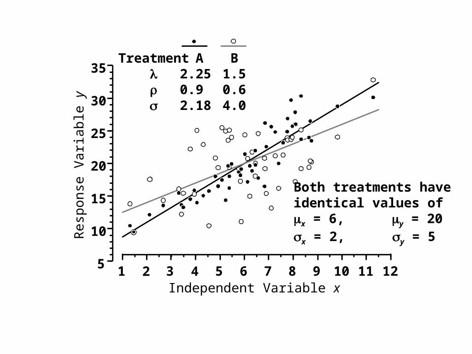
Measures of association between continuous variables
Correlation vs. linear regression
5
10
15
20
25
30
35
2 4 6 8 10 12Independent Variable x
Re
spo
nse
Var
iabl
e y
1 3 5 7 9 11
Treatment
A2.250.92.18
B1.50.64.0
Both treatments haveidentical values ofx = 6, y = 20x = 2, y = 5

x j
xj
yjj th Regression Error
Treatment Dose Level
RegressionLine x
1 Unitof
Dosage
0
Pat
ient
R
espo
nse
•

20
25
30
35
40
45
5 10 15 20 25 30Estriol (mg/24 hr)
Birt
hwei
ght (
g/10
0)
Rosner Table 11.1Am J Obs Gyn 1963;85:1-9
c) Slope parameter estimate
a.k.a. ) is estimated by b = r sy
/sx

r = 0
r = -1
0 < r < 1
r = 1
is estimated by b = r
sy /sx

20
25
30
35
40
45
5 10 15 20 25 30Estriol (mg/24 hr)
Birt
hwei
ght (
g/10
0)
Rosner Table 11.1Am J Obs Gyn 1963;85:1-9
Studies can be either experimental or observational

Normally distributed unless investigator
chooses level
Treatment level
Chosen by investigator

Estimating directly is often difficult
21/ 1x
2 2 2y x
=
=
If we can estimate
and x
Warning:
If the anticipated value of in your experiment is different from that found in the literature then your value of will also be different.
x
or and x y

5
10
15
20
25
30
35
2 4 6 8 10 12Independent Variable x
Re
spo
nse
Var
iabl
e y
1 3 5 7 9 11

Relationship between BMI and exercise time
n = 100 women willing to follow a diet exercise program for six months
Interquartile range (IQR) of exercise time = 15 minutes (pilot data) = (IQR / 2) / z0.25 = 7.5 / 0.675 = 11.11x
= 4.0 kg/m2 = standard deviation of BMI for women obtained by Kuskowska-Wolk et al. Int J Obes 1992;16:1-9
y
Would like to detect a true drop in BMI of = -0.0667 kg/m2 per minute of exercise
(1/2 hour of exercise per day induces a drop of 2 kg/m2 over 6 months)
a

When
0.675
0.250.25
-0.675
InterquartileRange
= (IQR / 2) / z0.25xIn general

Impaired Antibody Response to Pneumococcal Vaccineafter treatment for Hodgkin’s Disease
Siber et al. N Engl J Med 1978;299:442-448.
n = 17 patients treated with subtotal radiation. vaccinated 8 to 51 months later
A linear regression of log antibody response against time from radiation to vaccination gave
ˆ 0.01 0.11
0.40
P
r
Suppose we wanted to determine the sample size for a new study with
1 0.90
0.05
patients randomized to vaccination at 10, 30, or 50 weeks

Vit
al C
ap
aci
ty (
liters
)
Age (years)
Exposed > 10 years Unexposed
20 30 40 50 60
2
4
6
Composing Slopes of Two Linear Regressin Lines
Armitage and Berry (1994) gave age and pulmonary vital capacity for28 cadmium industry workers with > 10 years of exposure44 workers with no exposure

112x
29.19x
1̂ 0.0306
2̂ 0.0465
(unexposed)
(exposed)
pooled error variance
2 2 21 1 2 2 1 22 2 /( 4) 0.395
0.574
s s n s n n n
s
2 1ˆ ˆ 0.0159 ( 0.26)P
How many workers do we need to detect with
ratio of unexposed workers m = 44/28 = 1.57?
1 0.8, 0.05
Need 167 exposed workers and167 x 1.57 = 262 unexposed workers

112x
29.19x
1̂ 0.0306
2̂ 0.0465
(unexposed)
(exposed)
pooled error variance 2 0.395
0.574
s
s
2 1ˆ ˆ 0.0159 ( 0.26)P
How many workers do we need to detect with
ratio of unexposed workers m = 44/28 = 1.57?
2 1 0.0159 1 0.8, 0.05
Need 167 exposed workers and167 x 1.57 = 262 unexposed workers