![Data Glitches = Constraint Violations – Empirical …Divesh Srivastava AT&T Labs-Research A spaceman's word for irritating disturbances [Time, 23 Jul 1965]. ... – Data glitches](https://static.fdocuments.us/doc/165x107/5f08c5587e708231d423a432/data-glitches-constraint-violations-a-empirical-divesh-srivastava-att-labs-research.jpg)
$ G Y D Q F H V LQ P R G H OV R I 3 X OV D U * OLWF K H V 7 Measuring neutron star masses with...
190
Transcript of $ G Y D Q F H V LQ P R G H OV R I 3 X OV D U * OLWF K H V 7 Measuring neutron star masses with...

Advances in models of Pulsar GlitchesStefano L. Seveso
Physics, Astrophysics and Applied Physics PhD SchoolUniversità degli Studi di Milano
Advances in models of Pulsar Glitches
Neutron stars are surely one of the most interesting astronomical objects: in no other place of the observable universe, in fact, matter is so compressed that the density reaches and overcomes the nuclear saturation value. This is a so extreme condition that in no terrestrial laboratory we can directly re-produce it in order to study its properties. Neutron stars are therefore a very fascinating research field that can bring us to a deeper understanding of this exotic matter, by modeling the observations of peculiar phenomena rrelated to these stars. This thesis is focused on the pulsar glitches, which are rapid jumps in the rotation velocity of the star.
Shortly after the first glitches were observed it was suggested that they could be due to a superfluid component in the stellar interior that could store angular momentum thanks to the pinning interaction between super-fluid vortexes and crustal lattice. This qualitative idea suggests that the problem must be faced by merging results which come from the micro-physics point of view into a more macroscopic simulation. Therefore the mesoscopic calculation of the pinning force profiles is addressed, both for the crust of a neutron star and for the core. These results are used in static models which can reproduce the physical observable parameters.
The whole time evolution of a glitch can be followed thanks the develop-ment of a dynamical model. The multifluids formalism is implemented in a consistent simulation, which take into account realistic physical inputs like equation of state, entrainment and drag forces: the rise and the recovery of a glitch is analyzed in connection with the relevant parameters of the model. By comparing the results with the observational data, important aspects about this phenomenon and neutron stars in general are dis-cussed here.
Advances in m
odels of Pulsa
r Glitches
Seveso

Scuola di Dottorato in Fisica, Astrofisica e Fisica Applicata
Dipartimento di Fisica
Corso di Dottorato in Fisica, Astrofisica e Fisica Applicata
Ciclo XXVI
Advances in models ofPulsar Glitches
Settore Scientifico Disciplinare FIS/05
Supervisore: Professor Pierre M. PIZZOCHERO
Coordinatore: Professor Marco BERSANELLI
Tesi di Dottorato di:
Stefano L. SEVESO
Anno Accademico 2014

Commission of the final examination:
External Referee:Professor Jose A. Pons, Universitat d’Alacant, Departament de Fisica Aplicada
External Member:Professor Valeria Ferrari, Università di Roma La Sapienza, Dipartimento di Fisica
External Member:Professor Nicolas Chamel, Université Libre de Bruxelles, Institute of Astronomy andAstrophysics
Final examination:
Tuesday, January 20, 2015
Università degli Studi di Milano, Dipartimento di Fisica, Milano, Italy

A Daniela, Michela ed Eleonora...ovviamente...

MIUR subjects:
FIS/05 - Astronomia e Astrofisica
PACS:
97.60.Gb Pulsars97.60.Jd Neutron stars26.60.-c Nuclear matter aspects of neutron stars
Keywords: neutron stars, pulsars, glitch, Vela Pulsar, B0833-45, superfluidity, super-conductivity, snowplow model, neutron stars masses, pinning force, flux-tube, dragforce, mutual friction, dynamical model, two-fluids model
Contents
List of Figures iv
List of Tables vii
1 Introduction 1
2 Background concepts for superfluid glitch models 52.1 Neutron stars formation 52.2 Stellar structure 72.3 The role of superfluidity 132.4 Superfluidity in neutron star and entrainment effect 17
Part I: The pinning force 20
3 Crustal pinning 213.1 Introduction 213.2 Lattice properties 233.3 Mesoscopic pinning force 293.4 Results of the model 343.5 Conclusions 40
4 Core pinning 424.1 A simple approach 424.2 The realistic mesoscopic model 434.3 Results 494.4 Conclusions 55
i

Contents ii
Part II: The Snowplow model 58
5 The “snowplow” model 595.1 Pinning and vorticity 595.2 The model 625.3 Results and observations 685.4 Conclusions 74
6 Investigating superconductivity with the snowplow model 766.1 Introduction 766.2 The model 776.3 Results 806.4 Conclusions 82
7 Measuring neutron star masses with pulsar glitches 847.1 The entrainment in the snowplow paradigm 857.2 Fitting of NS masses with the snowplow model 907.3 A new analysis of the observational data 967.4 Observational data and the snowplow model 106
Part III: A dynamical model 111
8 The hydrodynamical model 1128.1 Introduction 1128.2 The multifluids formalism and neutron stars 1148.3 Mutual friction and equations of motion 1168.4 Physical inputs of the model 120
9 Results of the dynamical simulations 1279.1 Qualitative analysis of a simulation 1299.2 Parameter study 1349.3 Fit of the NS masses 1399.4 Conclusions 146
Conclusions and future directions 148
Appendices 150
A Rotational properties of neutron stars 151A.1 Magnetic dipole model 153

Contents iii
B Global two–components model 156
C Derivation of the multifluids formalism 159C.1 Introduction 159C.2 Multi–fluids systems: equations of motion 160C.3 Conservation laws 161C.4 Application to neutron stars 162
Bibliography 165

List of Figures
2.1 Diagram of the typical stellar evolution 62.2 Schematic representation of the forces in the hydrostatic equilibrium 82.3 Mass–radius relation for different equations of state 92.4 Mass–central density relation for the EoSs considered 102.5 Typical result of a TOV integration 112.6 Plot of the thicknesses of the different regions of a neutron star 142.7 Schematic representation of a vortex bundle 162.8 Pairing gap energy for superfluid matter in neutron star 18
3.1 Representation of a nucleus displacement in the nuclear pinning case 263.2 Representation of a nucleus displacement in the interstitial pinning case 273.3 Representation of the vortex deformation for pinning effect 283.4 Representation of the vortex rigidity on different scales 293.5 Number of captured pinning sites N(λ,κ) in the aligned case 313.6 Number of captured pinning sites N(λ,κ) in the non–aligned case 323.7 Difference between the number of pinning sites of the free and bound
configurations as a function of the vortex orientation 333.8 Convergence test for the l parameter used in our calculation of the
crustal pinning force 363.9 Convergence test for the dh parameter used in our calculation of the
crustal pinning force 373.10 The crustal pinning force per unit length for the β = 1 case 383.11 The crustal pinning force per unit length for the β = 3 case 393.12 Fit of the crustal pinning force as a function of the capture radius 40
4.1 Schematic representation of a vortex immersed in a regular lattice offlux–tubes 44
4.2 Number of captured pinning sites N(λ,κ) when the vortex is alignedwith the lattice 45
iv

List of Figures v
4.3 Number of captured pinning sites N(λ,κ) when the vortex is non–aligned with the lattice 46
4.4 Schematic representation of a vortex in the lattice with entanglement 484.5 Number of captured pinning sites N(λ,κ) in the entangled case 494.6 Convergence test for the parameters l and dh used in our calculation 514.7 Pinning force per unit length for L = 1000 Rws 524.8 Pinning force per unit length for L = 2500 Rws 534.9 Pinning force per unit length for L = 5000 Rws 534.10 Pinning force per unit length for L = 10 000 Rws 544.11 Plot of the fitting curves obtained (no entanglement) 544.12 Plot of the fitting curves obtained (with entanglement) 56
5.1 The profile of the pinning force fpin(ρ) used for calculations 605.2 A schematic representation of the geometry in the snowplow model 615.3 The total pinning force Fpin(x) integrated on the whole length of a vortex 635.4 Plot of the expression F∗m(x) = Fm(x)/∆Ω(x) as a function of the
cylindrical radius x 655.5 Plot of the critical lag ∆Ωcr(x) for different stellar models 66
6.1 Plots of the fractional step in frequency derivative ∆Ω/Ω for varyingvalues of the fraction of pinned vorticity in the core ξ 81
7.1 Plot of the entrainment effective neutron mass m∗n/mn as a function ofthe barion density nb 86
7.2 Critical lag profile and calculation of the angular momentum exchange 887.3 Plot of the curves ∆Ωgl(t) obtained with different values of the param-
eter Ygl 897.4 Plot of the curves ∆Ωgl(t) obtained with different values of the total
mass M of the star 907.5 Results of the fitting procedure for SLy (part 1) 927.6 Results of the fitting procedure for SLy (part 2) 937.7 Results of the fitting procedure for GM1 (part 1) 947.8 Results of the fitting procedure for GM1 (part 2) 957.9 Effect of the entrainment on the curves ∆Ωgl(t) used to fit the observa-
tional data 977.10 Number of glitch Ngl versus the spin–down parameter |Ω| for the con-
sidered pulsars 987.11 Maximal glitch jump ∆Ωglmax
versus the spin–down parameter |Ω| forthe considered pulsars 99
7.12 Average glitch jump ⟨∆Ωgl⟩ versus the spin–down parameter |Ω| for theconsidered pulsars 100
7.13 Average waiting time ⟨tgl⟩ between two consecutive glitches versus thespin–down parameter |Ω| for the considered pulsars 102

List of Figures vi
7.14 Plot of all measured events for the very frequent glitchers 1027.15 Glitch size ∆Ωgl versus the average lag ω for the considered pulsars 1047.16 Plot of the dispersion parameter ξ versus the average lag ω for the
considered pulsars 1057.17 Total observational lag ωobs = |Ω|Tobs versus the spin–down parameter
|Ω| for the considered pulsars 1067.18 Inferred mass M versus the lag parameter ω (SLy) 1087.19 Inferred mass M versus the lag parameter ω (GM1) 108
8.1 Plot of the drag profile for the crust 125
9.1 Diagram of the execution flow of the simulation code 1289.2 Plot of the rotational velocity of the crust versus time in the whole
simulation 1309.3 Typical lag profile at a given time between two glitches 1319.4 Effect of the entrainment in the hydrodynamical model 1329.5 Rise phase of a glitch and recovery effect 1339.6 Effect of the kelvonic drag parameter Bk 1359.7 Effect of the core drag parameter Bc 1369.8 Effect of the neutron fraction Q 1379.9 Effect of the parameter ηg 1389.10 Comparison of the residuals with observational data from Vela glitches 1399.11 Effect of the mass of the star M 1409.12 Effect of the triggering lag parameter ω∗ 1419.13 Effect of parameter η 1429.14 Plot of the ∆Ωp(t) curves of our best fits 1439.15 Inferred mass M versus the lag parameter ω (SLy) 1449.16 Inferred mass M versus the lag parameter ω (GM1) 1459.17 Plot of ∆Ωp(t) together with ∆Ωn(t) of our best fits 146
A.1 Radiation intensity profile measured by a radio telescope while observ-ing a pulsar 152
A.2 Representation of the magnetic field of a pulsar with the radiation beam 152A.3 P P diagram of all the known pulsars 155
B.1 Schematic representation of a glitch 158
List of Tables
2.1 Maximum allowed mass with the corresponding central density for theEoSs considered 11
2.2 Structural parameters of the stars used to test our models 13
3.1 Fiducial values of the NS crustal properties used in our calculations ofthe pinning force 24
3.2 Lattice properties for the five zones of the NS crust considered for thepinning force calculations 28
3.3 Results of the crustal pinning force calculations for vortexes with lengthL up to 5000Rws 35
3.4 Fit parameters for the pinning force 39
4.1 Fit parameters for the pinning force 554.2 Results for the pinning force per unit length for a pulsar and for a
magnetar 57
5.1 Fitting parameters fPM and Ygl for all the considered configurations andproton fraction xp = 0.05 69
5.2 Fitting parameters fPM and Ygl for all the considered configurations andproton fraction by Zuo et al. (2004) (two–body forces) 70
5.3 Fitting parameters fPM and Ygl for all the considered configurations andproton fraction by Zuo et al. (2004) (three–body forces) 71
5.4 Result of the snowplow model for all the considered configurations andproton fraction xp = 0.05 72
5.5 Result of the snowplow model for all the considered configurations andproton fraction by Zuo et al. (2004) (two–body forces) 73
5.6 Result of the snowplow model for all the considered configurations andproton fraction by Zuo et al. (2004) (three–body forces) 74
vii

List of Tables viii
7.1 Results of the fitting procedure: the inferred values of the masses offrequent glitchers 96
7.2 Observational values for the pulsars used in this work 110
9.1 Results of the fitting procedure: the inferred values of the masses offrequent glitchers 144

CHAPTER 1Introduction
Neutron stars are surely one of the most interesting astronomical objects: in no otherplace of the observable universe, in fact, matter is so compressed that the densityreaches and overcomes the nuclear saturation value. This is a such extreme conditionthat in no terrestrial laboratory we can directly reproduce it in order to study itsproperties. Neutron stars are therefore a very fascinating research field that can bringus to a deeper understanding of this exotic matter, by modeling the observations ofpeculiar phenomena related to these stars. In this work we focus on the pulsar glitches,which are rapid jumps in the rotation velocity of the star. Even if pulsars are known tobe very stable clocks, many of them show sudden increase in their spin frequency thatare instantaneous to the accuracy of the data.
To date several hundreds of glitches have been detected, with relative increasesin the spin frequency ν that range from as low as ∆ν/ν≈ 10−11 to ∆ν/ν≈ 10−5. Inparticular a class of pulsars, of which the Vela pulsar is the prototype, exhibit what areknown as “giant” glitches (Espinoza et al., 2011), large steps in the spin frequency(∆ν/ν ≈ 10−6) which are accompanied by an increase in the spindown rate ν andexhibit a rough periodicity in their recurrence rate (for example giant glitches in theVela occur roughly every three years).
Shortly after the first glitches were observed it was suggested that they could bedue to a superfluid component in the stellar interior, weakly coupled to the normalcomponent and to the electromagnetic emission, that could store angular momentumand then release it catastrophically, giving rise to a glitch (Baym et al., 1969; Andersonand Itoh, 1975; Alpar, 1977; Alpar et al., 1984b). Large scale superfluid componentsare, in fact, expected in neutron star interiors on theoretical grounds. The qualitativepicture can be explained by considering that a superfluid rotates by forming an array ofquantized vortexes which carry the circulation of the fluid. In the NS crust the vortexescan be strongly attracted, “pinned”, to the nuclear lattice (Pines et al., 1980; Andersonet al., 1982) and cannot move outward. If the superfluid cannot remove vortexes itcannot spin down and it therefore acts as an angular momentum reservoir. As the crustspins down due to electromagnetic emission a lag will develop between the superfluid
1

Chapter 1. Introduction 2
and the normal component, leading to a hydrodynamical lift force (Magnus force)acting on the vortexes. Eventually when the lag reaches a critical value the pinningforce will no longer be able to contrast the hydrodynamical lift and the vortexes willunpin, transferring their angular momentum to the crust and giving rise to a glitch.
Although there is some evidence that smaller glitches in young active pulsars (likeCrab) may be related to crust quakes, there is a growing consensus that the basicidea outlined above can be used to describe the main features of pulsar glitches. Inthis work we want to propose models which implement the superfluid frameworkrealistically in order to reproduce the physical observable parameters of the event.
The picture outlined above indicates that the problem must be faced by mergingresults which come from the microphysics point of view into a more macroscopicsimulation. Our research has been developed in parallel on these complementaryaspects and the structure of the thesis reflects this approach. After the introductoryChapter 2, where we review the background concepts on which the models are built(superfluidity, hydrostatic equilibrium, TOV integration, stellar structure, entrainment),contents are divided in three main parts, described here.
Part I The first part of the thesis is focused on the microphysical ingredients of theproblem, in particular on the pinning interaction. One of the main difficultiesin performing calculations about glitches is the relative scarcity of realisticestimate of the pinning force between vortexes and nuclei, addressed on themesoscopic scale. Although some authors have performed realistic calculationsof the interaction between a vortex and a single nucleus of the lattice, theevaluation of the pinning force per unit length haven’t been tackled deeply, andsome work is required to fill this gap. In this part we propose our averagingprocedure that allow us to move from the pinning per site towards the force overthe whole vortex, which is the relevant quantity of the superfluid models. Wecall this approach “mesoscopic” because it’s the fundamental bridge which bringsour knowledge about nuclear physics into a macroscopic model of glitches.
Chapter 3 In this chapter we use the vortex–site interaction results of Donatiand Pizzochero (2004, 2006) to propose the first realistic estimate of thepinning force per unit length in the inner crust of a neutron star. We takeinto account all possible vortex–lattice orientations and we obtain a forcefcrust ∼ 1015 dyn/cm, nearly two orders of magnitude less than previousnaive estimates.
Chapter 4 If protons in the interior of NS are in a type II superconductingstate, an interaction between magnetic flux tubes and rotational vortexesis possible and must be estimated (in case of type I superconductivity theinteractions are much weaker). The same qualitative approach used forthe crust is adopted also in this chapter to perform a calculation of thepinning interaction per unit length in the core of a neutron star. Our resultsindicate that even if the superconductivity is of type II, the interaction

Chapter 1. Introduction 3
between vortexes and flux tubes will be significantly weaker than in thecrust, because the force per unit length is fcore ∼ 1012–1013 dyn/cm.
Part II The second part of the thesis is focused on static models of pulsar glitches,in particular the snowplow model. The pinning profiles of chapter 3 are im-plemented, together with spherical geometry and realistic background, in amacroscopic model that provides interesting hints about the interior of neutronstars.
Chapter 5 In this chapter the snowplow model of Pizzochero (2011) is imple-mented using realistic equations of state and therefore realistic densityprofiles for the pulsars. In this chapter we don’t consider a pinning inter-action in the core, thanks to the results of chapter 4. The main goal is toreproduce the typical order of magnitude of the observable quantities thatare relevant in a giant glitch. The model described naturally explains theangular momentum storing mechanism that is responsible of the glitch,with minimal assumptions on the dynamic of vortexes. We find that theresults are in agreement with observations and support the outcome ofchapter 3 ( fcrust ∼ 1015 dyn/cm).
Chapter 6 Even if the results of chapter 4 indicates that the pinning in the coreof a pulsar is negligible, in this chapter we try to estimate with the snowplowmodel (with realistic physical inputs) what happens if a variable fractionof vorticity is blocked in the core by a strong pinning–like interaction. Bycomparing the results of the model with the observational data of theVela 2000 glitch (step in frequency and in frequency derivative), we haveconstrained the pinned fraction of the core superfluid. Our conclusion isthat both quantities cannot be fitted if a considerable fraction of vorticity isblocked: this means that either most of the core is a type I superconductoror the vortex/flux–tube interaction is very weak, in agreement with themesoscopic result of chapter 4.
Chapter 7 Although there is still considerable debate on the real nature of the“trigger” of a glitch and several mechanisms have been proposed, we cananyway use the snowplow model to evaluate the amount of the angularmomentum exchange as a function of the interglitch time between twoevents. By including also the entrainment in our calculations, this approachlet us to fit well the observational data and infer the masses of the mostfrequent glitching stars. The model proposed in this chapter gives a unifieddescription of the glitch phenomenon both for small and large glitchers andindicates an interesting correlation between mass and glitching strength.
Part III The last part of the thesis is focused on the development of dynamical modelwhich can follow the whole time evolution of this phenomenon. We implementthe multi–fluids formalism developed by Prix (2004); Andersson and Comer

Chapter 1. Introduction 4
(2006) in a consistent computer code, following the same approach of Haskellet al. (2012c), but using also realistic equations of state and the pinning profilesobtained in chapter 3. Moreover the entrainment effect is fully included inthe model together with the most realistic benchmarks for the mutual frictionbetween the components.
Chapter 8 In this chapter we derive the required formalism and describe indetail all physical ingredients of the model, like pinning, drag forces andentrainment, and how these inputs are encoded in the simulations.
Chapter 9 The results of the simulations are presented in this last chapter. Themodel allows us to study both the rise of a glitch and the recovery phaseand analyze the dependency of these behaviors on the drag parametersused in the calculation. We perform a parameter study for the relevantphysical quantities in order to understand more deeply all the aspects ofthis phenomenon. We also compare our simulations with the observationaldata of the frequent glitchers in order to estimate the masses of the pulsars.It’s noteworthy the fact that the results are in good agreement with the onesof chapter 7, showing again the same mass–glitching strength relation.

CHAPTER 2Background concepts forsuperfluid glitch models
Neutron stars are commonly classified by the modern astrophysics as “compact object”for their exceptional density. If we look at the macroscopic characteristics we canimmediately understand how strange these stars are. A typical neutron star in facthas a mass of the order of (1÷2)M but its radius is 105 times smaller (only about10km): this results in a very high central density that overcomes the value of thenuclear density ρ0 = 2.8g cm−3, unreachable in any other place of the universe.
To construct models of pulsar glitches we must know the properties of matterat these densities: in other words we must have a valid equation of state that canbe integrated to obtain the density profile inside the star. The high density is alsoresponsible of the presence of superfluid matter inside the core of the star: this fact isvery important for us because in this work we will focus on models that use preciselythe superfluidity to explain the glitch phenomenon.
2.1 Neutron stars formation
The formation of a NS can be considered the last step of the entire evolution of anormal star that begins with its formation from a gas cloud. If the mass of this gasreaches a critical value, the conditions for the existence of a self–gravitating objectare satisfied and the protostar begins its life. The Big Bang has produced a universecomposed mainly by hydrogen (75%) and helium (25%) so we can consider that thecloud has the same composition. We have
EG = −GM2
REK =
32
NkbT (2.1)
where EG is the gravitational energy of the cloud and EK is the kinetic energy (assumingan ideal gas). In these equations M is the total mass involved in the process, R its
5

Chapter 2. Background concepts for superfluid glitch models 6
GAS CLOUD
MAIN SEQUENCE STAR
RED GIANT
FUSION OF HEAVY ELEMENTSSUPERNOVAE
BROWN DWARF
WHITE DWARF
BLACK HOLENEUTRON STAR
M < 0.085 M
M < 0.5 M
M < 8 M
Figure 2.1: Diagram of the typical stellar evolution: the initial mass controls the entire life ofa star. The neutron star is a possible final phase if the core mass is below of the critical valuefor the black hole collapse.
radius and T the temperature. The crucial condition for the star formation is that|EG|> EK that lead us to the following critical values:
M > MJ ≡3kbTR2Gm
(2.2)
R< RJ ≡2GmM
3kb(2.3)
ρ > ρJ ≡3
4πM2
3kbT2Gm
2
(2.4)
These values are commonly know as the Jeans’ mass, radius and density.If these conditions are met, there is a first phase of free collapse due to the fact that
the loss in gravitational energy is used in the dissociation of the hydrogen molecules(H2 + γ→ H + H) and in the following ionization of the atoms (H + γ→ H+ + e−).When the hydrogen is totally ionized, the hydrostatic equilibrium condition is reachedand the protostar phase is completed. If the involved mass if above the threshold of0.08M the internal temperature of the object (which increase during the collapse)is enough to trigger nuclear fusion reactions. The longer phase of the life of the starbegins now, and it’s characterized by the conversion of hydrogen in helium: the star issaid to be in “main sequence”. When the core exhausts the reservoir of hydrogen, thestar begins to evolve in order to restore the equilibrium: the outer envelope expands,while the inner part compresses as a consequence of the reduction of the rate of nuclearreaction; therefore the temperature rise triggers the fusion of helium in heavier nucleibringing the star into a new burning phase. The whole life of the star is determined bythe initial mass: if it’s above the threshold of ≈ 8M the process repeats several times,

Chapter 2. Background concepts for superfluid glitch models 7
using each time the product of the previous phase, until the core of the star is madeup of iron (if the initial mass is below the threshold, the star becomes a white dwarf,sustained by the electron degeneracy pressure). At this point, no nuclear reaction isenergetically favorable and the core collapses in a hot, dense, neutron rich sphere ofabout 30 km, thanks to a fast neutronization process which produces a very high fluxof neutrinos. This collapse is eventually halted by the short range nuclear force, whilethe outer parts of the star are involved in the process known as supernovae explosion.
Neutron stars are one possible end point of this evolution, when the remainingcore is not too massive to overcome the neutron degeneracy pressure and becoming ablack hole. This threshold is Mmax and is about 2M; we will discuss this aspect later.The process described explains the name given to these objects: thanks to the inverseβ–reactions most of protons and electrons are transformed in neutrons which form ahigh density degenerate gas.
2.2 Stellar structure
In this work we are interested in the glitch phenomenon that schematically is theexchange of angular momentum between the superfluid part of the star and the normalone (this aspect will be covered deeply later, see section 2.3). Is therefore importantto calculate precisely the moment of inertia of the star and the distribution of matter(normal and superfluid) inside the compact object: in other words we must know thestellar structure.
The first step is to consider the hydrostatic equilibrium of the star. A neutron stardoesn’t collapse on itself and this means that exists a balance between the pressure andthe gravitational force, in every point on the star. If we look at the figure section 2.2we can see that a generic dV element at distance r from the center is subjected to agravitational acceleration that can be written as
g(r) =Gr2
∫ r
0
4πr ′2ρ(r ′)dr ′ (2.5)
due to the fact that, for the Gauss theorem, the gravitational attraction in sphericalsymmetry at distance r is given only by the enclosed mass; here in fact ρ(r) is thematter density. On the other hand, the force consequent to the pressure P acting ofthe element is
Fp(r) = P(r + dr)dA− P(r)dA= dA
dPdr
=dPdr
dV (2.6)
that produce an acceleration
ap(r) =dPdr
dVdm=
1ρ(r)
dPdr
(2.7)

Chapter 2. Background concepts for superfluid glitch models 8
r
P(r)Fg
P(r + dr)
dr
Figure 2.2: Schematic representation of theforces involved in the hydrostatic equilib-rium: the gravitational force is balanced bythe pressure inside the star.
The condition that the resulting force must be null leads us to the equation of thehydrostatic equilibrium in the newtonian case:
dPdr(r) = −ρ(r)
Gm(r)r2
(2.8)
2.2.1 TOV equations
Until now we have ignored the relativistic effects on the gravitational force. Anywayfor a neutron star GM/R ≈ 0.2c2 and therefore these aspects must be taken intoaccount. A full relativistic analysis of the hydrostatic equilibrium has been done byTollman, Oppenheimer and Volkoff with the following set of equations (known as theTOV equations):
dm(r)dr
= 4πr2ρ(r) (2.9)
dφ(r)dr
=
Gm(r)r2
+ 4πGrP(r)c2
1−2Gm(r)
c2r
−1
(2.10)
dP(r)dr
= −
ρ(r) +P(r)c2
dφdr
, (2.11)
where m(r) is the mass contained in a sphere of radius r, ρ(r) is the density profile andP(r) is the pressure. As already said, these differential equations model the hydrostaticequilibrium inside the star with relativistic approach and, of course, require the P(ρ(r))function. The last two equations can be combined in one that gives an expressionfor the mass and pressure derivatives and the system can be solved with valid initialconditions. We obtain the functions that describe the star with the fourth–order Runge–Kutta method, starting at r = 0 with m(0) = 0 and ρ(0) = ρc , for a valid choice of thecentral density ρc . The integration stops when we reach the condition ρ(R) = 10−8ρcand we take R as the radius of the star. Of course the mass of the star is M = m(R).

Chapter 2. Background concepts for superfluid glitch models 9
0
0.5
1
1.5
2
2.5
3
6 8 10 12 14 16 18
M [
MΟ•]
R [km]
POLFPSSLY
GM1GM3
AAU
CFPS2
UUWS
causalityrotation NR
Figure 2.3: Mass–radius relation for different equations of state. Each EoS implies a precisevalue of the maximum mass for a neutron star. In this work we will consider SLy (moderate)and the stiffer GM1. References for the other EoSs can be found at http://www.gravity.phys.uwm.edu/rns/source/eos/
2.2.2 EoS and integration of TOV equations
The function P(ρ(r)) is called the equation of state (EoS) because is the relationbetween pressure and density and it is therefore linked to the microphysic at thetypical densities of a NS. The formulation of a realistic EoS is a very challenging task,especially at so high densities: we cannot conduct an experiment to measure thepressure for such values of ρ. This means that an EoS is the result of a theoreticalmodel about the microscopic nature of matter and depends strongly on the assumptionsused. In literature there are many EoS and each one results in a different mass–radiusM(R) relation as we can see in fig. 2.3 This figure clearly identifies also the presenceof a limit for the mass for a neutron star. The existence of a maximum mass Mmax isan effect of the relativistic nature of the TOV equations, where pressure contributes tothe gravitational field: above the critical value, the pressure required to contrast thecollapse increases, in turn, the field and the object became a black hole (moreoverthe EoS can’t violate causality requirement, as showed by the upper shaded regionof fig. 2.3: the speed of sound must be less then the speed of light). Of course Mmaxdepends on the EoS: a stiffer equation of state gives a higher Mmax. The evidence ofthe existence of a 2 M neutron star (Demorest et al., 2010) allows, in fact, to rejectsoft equations of state that predict a maximum mass below this value. The fig. 2.3

Chapter 2. Background concepts for superfluid glitch models 10
0
0.5
1
1.5
2
2.5
0 2 4 6 8 10 12 14
M [
MΟ•
]
ρc [ρ0]
SLy GM1
Figure 2.4: This plot shows the mass–central density relation for the EoSs considered. Asexpected, we find a maximum mass value above 2 M for each equation of state (see table 2.1).
indicates that there is a minimum mass for a neutron star (lower shaded region):below this limit the gravitational attraction is not enough to resist to the centrifugalforce.Therefore we have decided to use these two different EoSs:
1. SLy (Douchin and Haensel, 2001) is a moderate EoS, based on a non–relativisticparametrisation; this equation describes the whole star with a single analyticalexpression and so it is more convenient to integrate;
2. GM1 by Glendenning and Moszkowski (1991) is a stiff P(ρ) relation that is verysimilar to SLy in the crust of star, but not in the core due to different microscopicapproach used to describe hadrons at densities higher than ρ0.
The fig. 2.4 shows the relation between the central density chosen as the initialcondition for the TOV integration and the resulting final mass, showing again theexistence of a limit mass Mmax (see table 2.1 for numerical details). Considering twostars with the same total mass M , we can see in fig. 2.5 how the choice EoS affect theresulting star obtained after the TOV integration: the stiffer EoS (GM1) requires alower central density and produce a larger radius. In this work we consider stars withmasses from 1M to Mmax.
The interior of a neutron star can be divided in three shell shaped regions, eachone characterized by a different composition. The outermost layer is called the outer

Chapter 2. Background concepts for superfluid glitch models 11
05.0⋅1032
1.0⋅1033
1.5⋅1033
2.0⋅1033
2.5⋅1033
0 2.0⋅105 4.0⋅105 6.0⋅105 8.0⋅105 1.0⋅106 1.2⋅106 1.4⋅106
m(r
) [g
]
r [cm]
02.0⋅10344.0⋅10346.0⋅10348.0⋅10341.0⋅10351.2⋅1035
P(r)
[dy
n cm
-2]
0
2.0⋅1014
4.0⋅1014
6.0⋅1014
8.0⋅1014
1.0⋅1015
ρ(r)
[g
cm-3
]
SLYGM1
Figure 2.5: This plot shows the result of the TOV integration performed with SLy and GM1in order to obtain a star of 1.4M. We can see how the stiffness of the EoS controls thedependency on the radius r of the density ρ, the pressure P and the contained mass m.
Table 2.1: This table shows, for each EoS, the maximum allowed mass with the correspondingcentral density ρc (in units of nuclear saturation density ρ0), radius of the star R, radius ofthe core Rc and radius of the inner crust Ric.
EoS ρc M R Rc Ric(ρ0) (M) (km) (km) (km)
SLy 10.2 2.04 9.98 9.68 9.86GM1 7.1 2.35 11.98 11.57 11.82

Chapter 2. Background concepts for superfluid glitch models 12
crust and it’s composed mainly by iron and heavier nuclei which are arranged in aBCC lattice (the electrons form a degenerate gas); the Coulomb interaction betweensites is very strong and this results in a very rigid crust, with thickness of ® 1 km.In this region matter is neutron–rich thanks to the inverse β–decay, but it’s still innormal state because the density is not enough to produce superfluid condensates.The EoSs in this layer are constructed by taking into account the contributions to thetotal energy density that come from the electrons, lattice structure and of course thenuclei. This last term is generally based on the standard “liquid drop model”.
The outer crust ends at the neutron drip density point ρd ≈ 4× 10¹¹ g/cm3. Abovethis point the nuclei become unstable and release free neutrons: the BCC lattice istherefore immersed in a degenerate neutron superfluid. This region is the inner crust(≈ 1 km thick) in which coexists matter in normal and superfluid state. The modelused for the outer crust to describe matter must be improved to consider this particularcondition: the energy density expression gains another term to encompass the freeneutron gas and for the nuclei the “compressible liquid drop model” is adopted (thisapproach takes into account the influence of the increase of density).
When the density approaches the nuclear saturation value ρ0 ≈ 2.8× 10¹⁴ g/cm3,nuclei dissolve gradually in a homogeneous n–p–e gas. This transition phase is called“pasta phase” (because nuclei are deformed away from the spherical geometry) and itmarks the beginning of the core, which contains most of the matter of the neutron star.In the inner part of the core, where density is highly above the saturation point, moreexotic forms of matter are possible, like pions, hyperons and maybe even deconfinedquarks: this is the most unknown region and all these considerations explain why it’sdifficult to describe precisely matter at so high density and why so many differentEoSs has been proposed.
Thanks to the TOV integration, we obtain the density profile ρ(r) and thereforeit is possible to identify, for each star, the structural regions that are relevant for ourmodels. In particular we calculate the radius of the core Rc as the distance from thecenter of the star where ρcore = ρ(Rc) = 0.5ρ0 (we fix ρ0 = 2.8g/cm3); the innercrust–outer crust interface Ric corresponds, on the other hand, to the density valueρd = 0.0015ρ0 that is the neutron drip point. It is easy also to calculate the momentof inertia of a shell delimited by radii r1 and r2:
I(r1, r2) =8π3
∫ r2
r1
r4ρ(r) dr. (2.12)
We can then calculate also the moment of inertia of every region, considering thatIcore = I(0, Rc), Iic = I(Rc , Ric) and Ioc = I(Ric, R).
Table 2.2 shows all the relevant parameters for the considered stars, obtained fromthe integration of the TOV equations with SLy and GM1.

Chapter 2. Background concepts for superfluid glitch models 13
Table 2.2: We give all the structural parameters (as defined in section 2.2.2) of the stars usedto test our models, for both EoSs tested. See also fig. 2.6 for a graphical representation ofthese quantities.
EoS M R Rc Ric Itot Icore Iic Ioc
(M) (km) (km) (km) (1045 gcm2) (1045 g cm2) (1043 gcm2) (1040 g cm2)
SLy 1.0 11.86 10.35 11.23 0.739 0.697 4.181 6.6381.1 11.83 10.49 11.28 0.827 0.788 3.923 5.9451.2 11.80 10.60 11.31 0.914 0.878 3.652 5.3171.3 11.76 10.69 11.32 0.999 0.965 3.370 4.7381.4 11.71 10.75 11.32 1.079 1.048 3.078 4.1981.5 11.64 10.79 11.29 1.154 1.126 2.777 3.6851.6 11.55 10.79 11.24 1.222 1.197 2.469 3.1941.7 11.42 10.76 11.16 1.279 1.258 2.150 2.7181.8 11.26 10.68 11.03 1.322 1.303 1.818 2.2481.9 11.03 10.54 10.83 1.339 1.324 1.463 1.7692.0 10.62 10.23 10.47 1.299 1.289 1.042 1.233
GM1 1.0 13.94 11.79 13.02 1.021 0.896 12.505 19.0611.1 13.94 12.01 13.12 1.146 1.025 12.068 17.5321.2 13.94 12.19 13.20 1.271 1.156 11.555 16.1081.3 13.93 12.35 13.27 1.395 1.285 10.991 14.7801.4 13.91 12.47 13.32 1.516 1.412 10.382 13.5301.5 13.89 12.58 13.34 1.634 1.536 9.738 12.3401.6 13.85 12.66 13.35 1.747 1.657 9.062 11.1981.7 13.79 12.71 13.35 1.854 1.771 8.362 10.0991.8 13.72 12.74 13.32 1.954 1.878 7.635 9.0311.9 13.62 12.74 13.26 2.043 1.974 6.885 7.9872.0 13.49 12.70 13.17 2.118 2.057 6.107 6.9562.1 13.33 12.63 13.05 2.173 2.120 5.292 5.9222.2 13.10 12.48 12.85 2.194 2.150 4.411 4.8512.3 12.71 12.20 12.51 2.146 2.113 3.371 3.631
2.3 The role of superfluidity
To understand the underlying mechanism of a glitch is necessary to frame some of theproperties of a superfluid because, in the models discussed here, they are responsiblefor this phenomenon. The superfluidity is a special condition of the fluids in which theydo not show signs of internal friction (viscosity). If we consider a fluid in the groundstate (T = 0) flowing through a container, its energy can be expressed in the referenceframe of the container to be due only by the kinetic contribution. If we suppose that asimple excitation arises in the fluid, we can characterize that by a momentum p andan energy contribution of ε(p); then the total energy will be of course
E =12
M v2 + ε(p) + p · v (2.13)
where we recognize the kinetic term (first one) and the change in energy due to theappearance of the excitation, ε(p) + p · v. This change must be negative because

Chapter 2. Background concepts for superfluid glitch models 14
1.00⋅106
1.05⋅106
1.10⋅106
1.15⋅106
1.20⋅106
1.25⋅106
1.30⋅106
1.35⋅106
1.40⋅106
0.8 1 1.2 1.4 1.6 1.8 2 2.2 2.4
R [
cm]
M [ MΟ• ]
SLy GM1
9.50⋅105
1.00⋅106
1.05⋅106
1.10⋅106
1.15⋅106
1.20⋅106
1.25⋅106
1.30⋅106
0.8 1 1.2 1.4 1.6 1.8 2 2.2 2.4
Rc
[cm
]
M [ MΟ• ]
SLy GM1
2.00⋅104
4.00⋅104
6.00⋅104
8.00⋅104
1.00⋅105
1.20⋅105
1.40⋅105
0.8 1 1.2 1.4 1.6 1.8 2 2.2 2.4
Inne
r cr
ust
thic
knes
s [c
m]
M [ MΟ• ]
SLy GM1
1.00⋅104
2.00⋅104
3.00⋅104
4.00⋅104
5.00⋅104
6.00⋅104
7.00⋅104
8.00⋅104
9.00⋅104
1.00⋅105
0.8 1 1.2 1.4 1.6 1.8 2 2.2 2.4
Out
er c
rust
thi
ckne
ss [
cm]
M [ MΟ• ]
SLy GM1
Figure 2.6: The first figure shows the dependence of the radius of the neutron star on thetotal mass, for the SLy and GM1 EoSs. The other plots represent the thicknesses of the stellarregions (core, inner crust and outer crust) as function of mass. As one can see, a more massivestar has thinner crusts, while a stiffer equation of state produces a larger star.
otherwise the excited state would not be energetically favored. Bearing in mind that pand v are antiparallel the algebraic relation is
v >ε(p)
p. (2.14)
It’s easy to verify that when ε(p) = p2
2m this condition is always satisfied, in otherwords there is no chance for the fluid to remain in its ground state. But in a fermionicsuperfluid, the excitation energy can be expressed as
ε(p) =
√
√
√
p2
2m
2
+∆2,
and this fact implies that the condition in eq. (2.14) can be rewritten as v >p
2m∆.(In a bosonic superfluid the excitation are phonons and this means that ε = csp andthen v > cs). In other words this means that if the velocity is below this threshold the

Chapter 2. Background concepts for superfluid glitch models 15
excitement does not occur and we can refer to this state as superfluidity. As we willsee in more detail, the presence of the dispersion term ∆ in the excitation energy, alsocalled pairing gap, it is crucial for the existence of superfluidity.
If we consider a superfluid in the ground state, we can describe its state with asingle wave function
ψ=p
n0 eiφ , (2.15)
where φ is a global phase factor, as |ψ|2 = n0. We can immediately draw someimportant general properties of this class of fluids that will be crucial to understandthe underlying mechanism of glitches. From quantum mechanics we know thatv= p
m = −iħh∇m , from which follows that
vψ= −iħh∇mψ= −i
p
n0ħhm
eiφ∇φ =ħhm∇φψ. (2.16)
This means that ħhm∇φ is an eigenvector of the velocity; for a Cooper pair m = 2mn andthen v= ħh
2mn∇φ. The result v∝∇φ implies that the macroscopic velocity field of a
superfluid is irrotational, because its curl is null: ∇× v =∇×∇φ = 0. In other wordswe can state that a superfluid will never rotate as a rigid body (namely ∇× v= 2Ω).
Consider now a cylinder rotating around its axis and a “normal” fluid inside,initially at rest: if there is a friction between the walls of the container and the fluid,this will be dragged and ultimately will rotate with its container. If instead we take asuperfluid, this is not possible and it will persist in its groud state, as shown before, aslong as this condition is thermodynamically favorable. In fact, if E is the total energyseen by a fixed “external” reference system, then when we move to the “rotating”coordinates, we have Erot = E −M ·Ω, where M is the angular momentum of the fluidand Ω is the rotational angular velocity of the container. The preferred thermodynamicstate is the one that minimizes Erot and we can see that if Ω is big enough, then itbecomes favorable a configuration with M 6= 0.
It’s important now to clarify the apparent contradiction with what has been ex-plained above, namely the fact that the superfluid has always ∇× v = 0 and thereforecan not rotate. The contradiction is resolved if we introduce singularities in the velocityfield. In other words, considering the circulation in place of the curl, we can write that
∮
Cv · dl= κ, (2.17)
where we consider a closed loop that encloses a straight singularity and it is centeredwith it. The value of the constant κ is obtained considering the relationship
∮
Cv · dl= κ=
ħh2mn
∆φ,
where ∆φ is the variation of the phase obtained by completing the circuit. Because ofcourse this amount must be an integer multiple of 2π, we have
κ= nπħhMN= n
h2mn
. (2.18)
Chapter 2. Background concepts for superfluid glitch models 16
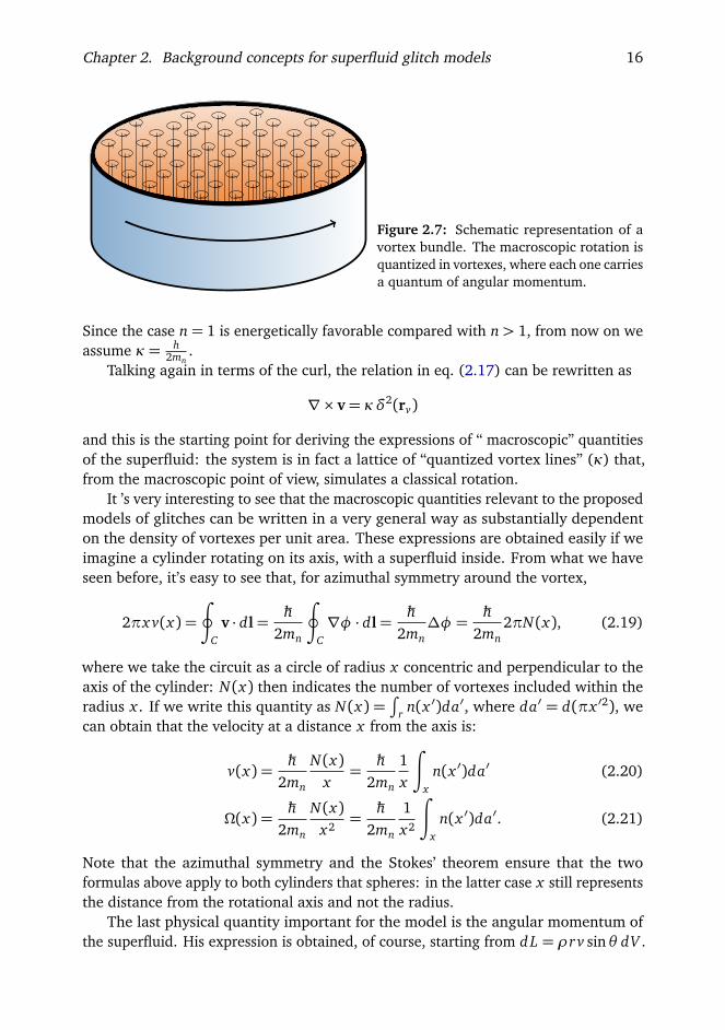
Figure 2.7: Schematic representation of avortex bundle. The macroscopic rotation isquantized in vortexes, where each one carriesa quantum of angular momentum.
Since the case n= 1 is energetically favorable compared with n> 1, from now on weassume κ= h
2mn.
Talking again in terms of the curl, the relation in eq. (2.17) can be rewritten as
∇× v= κδ2(rv)
and this is the starting point for deriving the expressions of “ macroscopic” quantitiesof the superfluid: the system is in fact a lattice of “quantized vortex lines” (κ) that,from the macroscopic point of view, simulates a classical rotation.
It ’s very interesting to see that the macroscopic quantities relevant to the proposedmodels of glitches can be written in a very general way as substantially dependenton the density of vortexes per unit area. These expressions are obtained easily if weimagine a cylinder rotating on its axis, with a superfluid inside. From what we haveseen before, it’s easy to see that, for azimuthal symmetry around the vortex,
2πx v(x) =
∮
Cv · dl=
ħh2mn
∮
C∇φ · dl=
ħh2mn
∆φ =ħh
2mn2πN(x), (2.19)
where we take the circuit as a circle of radius x concentric and perpendicular to theaxis of the cylinder: N(x) then indicates the number of vortexes included within theradius x . If we write this quantity as N(x) =
∫
r n(x ′)da′, where da′ = d(πx ′2), wecan obtain that the velocity at a distance x from the axis is:
v(x) =ħh
2mn
N(x)x=ħh
2mn
1x
∫
xn(x ′)da′ (2.20)
Ω(x) =ħh
2mn
N(x)x2
=ħh
2mn
1x2
∫
xn(x ′)da′. (2.21)
Note that the azimuthal symmetry and the Stokes’ theorem ensure that the twoformulas above apply to both cylinders that spheres: in the latter case x still representsthe distance from the rotational axis and not the radius.
The last physical quantity important for the model is the angular momentum ofthe superfluid. His expression is obtained, of course, starting from d L = ρrv sinθ dV .

Chapter 2. Background concepts for superfluid glitch models 17
If we consider a system with spherical symmetry, like a star with the density onlydependent on the radius, then the above equation is integrated in the following way:
L =ħh
2mn
∫
r,θ ,φ
ρ(r)N(r,θ )r sinθ dr dθ dφ. (2.22)
2.4 Superfluidity in neutron star and entrainment effect
A system of bosons, due to the fact that the excitations are phonons as described previ-ously, can condense into a ground state at low temperatures, manifesting superfluidproperties. Speaking instead of neutron stars, it is clear that we are interested in asuperfluid of fermionic type: the existence of a ground state is guaranteed thanks to theformation of Cooper pairs. Basically, the neutrons near the Fermi surface are correlatedin pairs so that they express bosonic features. The pairing gap ∆ corresponds preciselyto the binding energy per particle of these couples, and therefore it’s the gap betweenthe ground state and the first excited one. The value of this quantity is also linked tothe critical temperature of the superfluid from the relation kbTc = ∆(T = 0)/1.76.Above this temperature, the thermal energy is enough to break the pairs, bringingback the fluid to the “normal” condition.
Referring to what is described above with regard to the equation of state forneutron star matter, every region of the star has its own specific feature also in termsof superfluidity. The outer crust of course does not exhibit this behavior because, withthe density less than the drip value (ρd), there is no “free” neutrons that can organizeinto Cooper pairs and then condensate to the ground state. The situation is differentfor the inner crust and the core, where ρ > ρd . The Fermi energy is density dependentand therefore it’s easier for neutrons to form pairs: in the inner crust it’s only possiblethe formation of neutron superfluid (no proton superconductor is present here), whichare of type 1S0 (S wave), since this condition with antialigned spins maximizes thebinding energy, as shown by fig. 2.8. In the core, instead this state is possible onlyfor protons (for their lower density compared to neutrons), while neutrons will beorganized with the configuration 3P2: a hypothetical 1S0 pair would be broken by thenuclear repulsive interaction related to the high density, this does not happen in caseof aligned spin, because the p–wave scattering length for neutrons is longer than therepulsive range.
The superfluid condition indicates that the fluid can flow without internal friction,thanks to the existence of the pairing gap. Anyway, as we will consider a system madeup of two fluid (the superfluid and the “normal” one) for modeling NS glitches, wemust also take into account the possible interactions between the two species. Inchapter 8 we will consider the drag effects which are dissipative forces that occur bothin the core and in the crust of a neutron star and are responsible of the glitch dynamic.But there is also a non–dissipative effect that can’t be neglected: the entrainment. Theentrainment in the crust (in this work we will not consider non–dissipative entrainmenteffects for the core) is related to the elastic scattering of neutrons by the nuclear lattice.
Chapter 2. Background concepts for superfluid glitch models 18
0
0.5
1
1.5
2
2.5
3
0 0.05 0.1 0.15 0.2 0.25 0.3 0.35 0.4 0.45 0.5
Δ [
MeV
]
nb [fm-3]
neutron 1S0 proton 1S0
neutron 3PF2
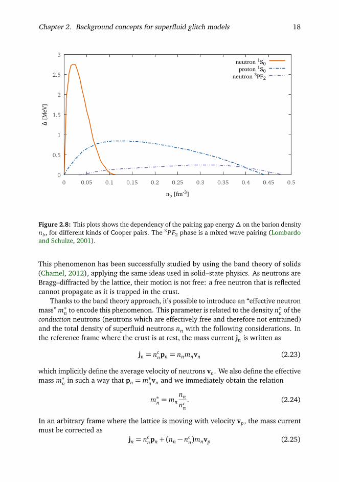
Figure 2.8: This plots shows the dependency of the pairing gap energy∆ on the barion densitynb, for different kinds of Cooper pairs. The 3PF2 phase is a mixed wave pairing (Lombardoand Schulze, 2001).
This phenomenon has been successfully studied by using the band theory of solids(Chamel, 2012), applying the same ideas used in solid–state physics. As neutrons areBragg–diffracted by the lattice, their motion is not free: a free neutron that is reflectedcannot propagate as it is trapped in the crust.
Thanks to the band theory approach, it’s possible to introduce an “effective neutronmass” m∗n to encode this phenomenon. This parameter is related to the density nc
n of theconduction neutrons (neutrons which are effectively free and therefore not entrained)and the total density of superfluid neutrons nn with the following considerations. Inthe reference frame where the crust is at rest, the mass current jn is written as
jn = ncnpn = nnmnvn (2.23)
which implicitly define the average velocity of neutrons vn. We also define the effectivemass m∗n in such a way that pn = m∗nvn and we immediately obtain the relation
m∗n = mnnn
ncn
. (2.24)
In an arbitrary frame where the lattice is moving with velocity vp, the mass currentmust be corrected as
jn = ncnpn + (nn − nc
n)mnvp (2.25)

Chapter 2. Background concepts for superfluid glitch models 19
because the fraction (nn − ncn) of “blocked” neutrons are moving with the crust. This
leads directly to equation
pn = m∗nvn + (mn −m∗n)vp = mn
vn + εn(vp − vn)
, (2.26)
where we have defined εn = (1−m∗n/mn). This relation shows that the neutron masscurrent is no longer aligned with neutron momentum, and this fact has importantconsequences over the superfluid dynamics, and therefore over the glitch, as we willtreat later in chapters 7 and 8. For a more detailed discussion about these aspects andthe multi–fluid formalism for a NS, see Carter et al. (2006); Andersson et al. (2006).
A realistic calculation of the densities nn and ncn has been performed by Chamel
(2012): the results indicate that in the intermediate part of the inner crust, whereρ ≈ 4.5× 10¹³ g/cm3, we have m∗n ≈ 14 mn. This means that most of the superfluidneutrons are actually entrained and therefore we cannot neglect this effect in ourmodels.

PART I
THE PINNING FORCE

CHAPTER 3Crustal pinning
The crust of a neutron star is thought to be comprised of a lattice of nuclei immersedin a sea of free electrons and neutrons. As the neutrons are superfluid their angularmomentum is carried by an array of quantized vortexes. These vortexes can pin to thenuclear lattice and prevent the neutron superfluid from spinning down, allowing it tostore angular momentum which can then be released catastrophically, giving rise to apulsar glitch. A crucial ingredient for this model is the maximum pinning force that thelattice can exert on the vortexes, as this allows us to estimate the angular momentumthat can be exchanged during a glitch. In this chapter we perform, a detailed andquantitative calculation of the pinning force per unit length acting on a vortex immersedin the crust and resulting from the mesoscopic vortex-lattice interaction. We considerrealistic vortex tensions, allow for displacement of the nuclei and average over allpossible orientation of the crystal with respect to the vortex. We find that, as expected,the mesoscopic pinning force becomes weaker for longer vortexes and is generallymuch smaller than previous estimates, based on vortexes aligned with the crystal.Nevertheless the forces we obtain still have maximum values of order fpin ≈ 1015
dyn/cm, which would still allow for enough angular momentum to be stored in thecrust to explain large Vela glitches, as will be deeply discussed in the next chapters.
3.1 Introduction
The physics of the Neutrons Star (NS) crust plays a crucial role when attempting tomodel these objects. First of all the outer layers of the star provide a heat blanketthat shields the hot interior and determines the observable thermal emission from thesurface (Gudmundsson et al., 1983). The elastic properties of the crust are also crucial,as “crust-quakes” have been invoked to explain a number of phenomena, such asmagnetar flares (Thompson and Duncan, 1995) and pulsar glitches (Alpar et al., 1994;Middleditch et al., 2006). Furthermore the crust may sustain a large enough strainto build a “mountain” that leads to detectable gravitational wave emission (Bildsten,1998). In this thesis we focus on the glitch phenomenon and therefore we want here
21

Chapter 3. Crustal pinning 22
to understand the role of the crust (in particular with the pinning interaction) in theseevents.
Glitches are sudden increases in frequency (instantaneous to the accuracy ofthe data) of an otherwise smoothly spinning down radio pulsar. Soon after thefirst observations, the long timescales associated with the post–glitch relaxation (upto months) were associated with the re-coupling of a loosely coupled superfluidcomponent in the NS crust (Baym et al., 1969). Neutron superfluidity in NS interiorsis, in fact, expected on a theoretical basis (Migdal, 1959) as most of the star will becold enough for neutrons to form Cooper pairs and behave as a superfluid condensate,that can flow with little or no viscosity relative to the ’normal’ component of the crust.
A crucial aspect of superfluid dynamics is that the neutron condensate can onlyrotate by forming an array of quantized vortexes, which determine an average rotationrate for the fluid. For the superfluid to spin-down it is necessary for vorticity to beexpelled. If vortexes are, however, strongly attracted to the ions in the crust (i.e. theyare ’pinned’) their motion is impeded and the superfluid cannot follow the spin-downof the crust, and stores angular momentum, releasing it catastrophically during aglitch (Anderson and Itoh, 1975).
The nature of the trigger for vortex unpinning is still debated, with proposalsranging from vortex avalanches (Alpar et al., 1996; Warszawski and Melatos, 2012b)to hydrodynamical instabilities (Glampedakis and Andersson, 2009) or crust quakes(Ruderman, 1969, 1976; Alpar et al., 1994; Middleditch et al., 2006). Whatever thetrigger mechanism, an important ingredient in this picture is the maximum pinningforce that the crust can exert on a vortex, before hydrodynamical lift forces (the Magnusforce) are able to free it. This quantity obviously determines the maximum amountof angular momentum that can be exchanged during a glitch. An understanding ofhow much angular momentum can be stored in different regions of the star would, infact, allow detailed comparisons with observations of glitching pulsars and potentiallyconstrain the equation of state of dense matter (Andersson et al., 2012; Chamel, 2013;Piekarewicz et al., 2014).
Early theoretical work focused on the microscopic interaction between a vortexand a single pinning site (Alpar, 1977; Epstein and Baym, 1988). The pinning forceper unit length of a vortex depends, however, on the mesoscopic interaction betweenthe vortex and many pinning sites, and thus on the rigidity of the vortex, on its radius(represented by the superfluid coherence length ξ) and on the lattice spacing. Thisnaturally leads to the possibility of different pinning regimes in different regions ofthe crust. Alpar et al. (1984a,b) interpreted the slow post-glitch recovery of the Velapulsar in terms of vortex “creep”, i.e. thermally activated motion of pinned vortexes,and distinguished between three regimes: strong, weak and super weak pinning. Thedifferent regimes depend on the interplay between the quantities mentioned earlier:in strong pinning the coherence length ξ of a vortex is smaller than the lattice spacing,and the interaction is strong enough to displace nuclei; while in the weak pinningregime this is not the case. Superweak pinning, on the other hand, comes about whenthe coherence length ξ is greater than the lattice spacing and a vortex can encompass

Chapter 3. Crustal pinning 23
several nuclei. In this case there is little change in energy as the vortex moves and thusno preferred configuration for pinning. The pinning force is expected to be weak and,in the limit of infinitely long vortexes all configurations are equal and there would beno pinning Jones (1991b). Fits to the post-glitch relaxation of the Vela pulsar, withinthe vortex creep framework (Alpar et al., 1984a), were used to set observationalconstraints on some of these parameters, leading to the conclusion that only weakand super weak pinning are likely to be at work in a neutron star crust (Alpar et al.,1984b). The theoretical calculations of the mesoscopic pinning force relied, however,on estimates in the weak pinning case for the very particular configuration of vortexesaligned with the crystal axis. Although very little is known about the defect structureof the crust, one does not in general expect the crystal lattice to be oriented in thesame direction over the whole length of a vortex (note also that a vortex will havecylindrical symmetry set by the rotation axis, while the only preferred direction forthe crystal will be set by gravity and pressure which have spherical symmetry, slightlymodified by rotation). More recently Link (2009) has performed simulations of motionof a vortex in a three-dimensional random potential, and found that the rigidity of thevortex does, indeed, play a fundamental role in setting the maximum superfluid flowabove which vortexes cannot remain pinned.
In this chapter we perform a realistic calculation of the mesoscopic pinning force,that is the force per unit length acting on straight vortexes in the neutron star crust. Weaverage over all possible vortex-crystal orientations and show that, although the forceis considerably weaker than previous estimates based on particular configurations, itcould still be strong enough to account for angular momentum transfer in large pulsarglitches.
3.2 Lattice properties
The crust of a NS is thought to form a crystal in which completely ionized neutron-richnuclei form a body centered cubic (BCC) lattice, immersed in a sea of electrons andfree neutrons. In this configuration each nucleus is at the center of a cubic cell ofside s = 2Rws with nuclei at each vertex. The separation between the ions (i.e. thepotential pinning sites) thus depends on Rws, the radius of the Wigner-Seitz cell, whichis a function of the density ρ. In our calculation we use the classic results from Negeleand Vautherin (1973) where the crust is divided in five zone, each one characterizedby a specific value of Rws and RN , which is the radius of the nucleus that occupies asingle site of the lattice. Table 3.1 summarizes these results, together with the nuclearcomposition of the Wigner-Seitz cells.
Note that there is still significant uncertainty on the exact composition and structureof the crust (Steiner et al., 2014; Piekarewicz et al., 2014) and not only electrons, butalso free neutrons, may partially screen the Coulomb interaction between the nuclearclusters, leading to different, and more inhomogeneous, configurations than a BCClattice (Kobyakov and Pethick, 2014). Nevertheless the procedure we describe below

Chapter 3. Crustal pinning 24
Table 3.1: Fiducial values of the quantities used in our calculations. These values are takenfrom Negele and Vautherin (1973): the NS crust is divided in five zone and here we givethe baryon density ρ, the Wigner-Seitz cell radius (Rws), the element corresponding to thecell nuclear composition, the nuclear radius (RN ), the superfluid coherence length (ξ), whichrepresents the vortex radius, and the pinning energy per site (Ep). The last two quantities aretaken from the results of Donati and Pizzochero (2004, 2006)
# ρ [g cm−3] Element Rws [fm] RN [fm] ξ [fm] Ep [MeV]
β = 1 β = 3 β = 1 β = 3
1 1.5× 10¹² 32040Zr 44.0 6.0 6.7 20.0 2.63 0.21
2 9.6× 10¹² 110050Sn 35.5 6.7 4.4 13.0 1.55 0.29
3 3.4× 10¹³ 180050Sn 27.0 7.3 5.2 15.4 -5.21 -2.74
4 7.8× 10¹³ 150040Zr 19.4 6.7 11.3 33.5 -5.06 -0.72
5 1.3× 10¹⁴ 98232Ge 13.8 5.2 38.8 116.4 -0.35 -0.02
can easily be adapted to different configurations.To calculate the mesoscopic pinning force we need to identify the configurations in
which the vortex is most strongly pinned to the lattice and the configurations in whichit is ’free’. Once this has been done the maximum pinning force Fp simply followsfrom:
Fp =Efree − Epin
∆r(3.1)
where Epin is the energy of the most strongly pinned configuration and Efree the energyof the free configuration. The average distance the vortex has to move between theconfigurations is ∆r.
The energy of a particular vortex configuration will depend on the number ofions that it is able to pin to. Intuitively, the more sites it can pin to, the greater theenergy gain, the stronger the pinning. In order to perform the calculation it is thusnecessary to consider the pinning energy per pinning site Ep, i.e. the amount by whichthe energy of the system is changed when a single nucleus is inside the vortex. Thisquantity depends on the competition between the kinetic energy and the condensationenergy of the superfluid, which is strongly density dependent and will thus change if adense nucleus is introduced in the vortex. In this work we use the results of Donatiand Pizzochero (2003, 2004, 2006), who calculate Ep consistently in the local densityapproximation. The values of Ep for different densities are given in the last columnsof table 3.1. Note that in some regions Ep is positive, i.e. it costs energy to introduce anucleus in a vortex. In these regions the vortex-nucleus interaction is repulsive and onehas ’interstitial’ pinning (IP), in which the favored vortex configurations are in-betweennuclei. We refer to the case in which the interaction between nuclei and vortexes isattractive as ’nuclear’ pinning (NP). We shall see in the following that the effect ofattraction or repulsion does not strongly influence the calculation of the mesoscopic

Chapter 3. Crustal pinning 25
pinning force. The parameter β refers to the suppression factor for the neutron pairinggap used in the calculations: ∆= ∆0
β , where ∆0 is the pairing gap of the superfluidobtained by using the bare interaction (i.e. not accounting for in-medium corrections).This factor is related to the polarization effects of matter on the nuclear interaction.The case β = 1 describes the non–polarized interaction, while the case β = 3 describesthe one in which the effect of the polarization is maximum. When β = 1 the meanpairing gap has a maximum of about 3 MeV, which corresponds to the strong pairingscenario, while when β = 3 the mean pairing gap has a maximum of about 1 MeV,as usually assumed in the weak pairing scenario. Realistic Montecarlo simulations ofneutron matter (Gandolfi et al., 2008) indicate a reduction of the pairing gap consistentwith the choice β = 3.
The total energy of the interaction between a given vortex portion and the latticeis calculated summing the contribution of each nucleus that can be captured by thepinning force. Naively this could be done by considering the vortex as a cylinder ofradius ξ and counting how many nuclei are contained within it (we will discuss howto count nuclei at the boundary in the following). This approach can be improvedto take into account the possible deformation of the nuclear lattice. The lattice haselastic properties, so it is possible for nuclei to be displaced from their equilibriumposition under the action of the pinning force. The resulting energy per site can beexpressed as
E(r) = Ep + El(r) (3.2)
where r is the distance of the vortex axis from the equilibrium position of the considerednucleus. In this approach, the pinning energy per site Ep is corrected by the factorEl(r) that encodes the change in electrostatic energy due to the displacement of thenucleus. We will then define the capture radius rc as the radius within which it isenergetically favorable for the nuclei to be displaced: this will be the radius of thevortex to be used in the counting procedure. Let us now estimate rc for both nuclearand interstitial pinning.
3.2.1 Nuclear pinning
In the nuclear pinning regime (Ep < 0) we define a pinning region assuming that anucleus contributes to the total interaction by a factor Ep if it is completely inside thevortex: in other words its distance from the vortex axis must be less than γ= ξ− RN(fig. 3.1). If a site is at a distance r > γ from the vortex axis, the nucleus must bedragged by a distance δ(r) = r−γ. The electrostatic energy is calculated in a standardway using Gauss theorem together with the Wigner-Seitz approximation, which dividesthe lattice in independent spherical cells of radius Rws each with an ion in the centersurrounded by the electron and neutron gas:
El(r) =Z2e2
2R3wsδ2(r) (3.3)

Chapter 3. Crustal pinning 26
r
r − γ
γ= ξ− RN Figure 3.1: Representation of a nucleus dis-placement (NP case). The empty and full cir-cles represent respectively the starting andfinal position of the nucleus. The dashedline represents the displacement δ(r).
where e is the elementary charge and Z is the number of protons and electrons in thecell. Of course, a nucleus whose equilibrium position is already inside the pinningregion does not need to be dragged, so its energy contribution has no electrostaticterm (E(r) = Ep if r < γ). We can now define the maximum drag distance r0 as thevalue of δ(r) for which the effective pinning interaction of eq. (3.2) becomes zero:
r0 =
√
√
−2EpR3
ws
Z2e2. (3.4)
From these consideration, it follows that the final capture radius that must be used inour calculation will be
rc = γ+ r0 = ξ− RN + r0 (3.5)
The total energy of the interaction between the considered vortex portion (oflength L) and the lattice is calculated summing the contribution of each nucleus thatcan be captured by the pinning force. This energy is calculated through an integralover a uniform distribution of nuclei, that is valid when the number of nuclei whichare taken into account becomes very large, so for L Rws. Given N the number ofpinning sites that fall inside a cylinder of radius rc and length L, the superficial densitywill be nN =
Nπr2
c. Then the total energy is calculated as
E =
∫ γ
0
EpnN 2πr dr +
∫ γ+r0
γ
Ep + El(r)
nN 2πr dr
=N Ep
(γ+ r0)2
γ2 +43γr0 +
12
r20
(3.6)

Chapter 3. Crustal pinning 27
r
γ− r
γ= ξ+ RN Figure 3.2: Representation of a nucleus dis-placement (IP case). The empty and full cir-cles represent respectively the starting andfinal position of the nucleus. The dashedline represents the displacement δ(r).
From this equation we can immediately evaluate the effective interaction energy persite Eeff, defined by E = N Eeff:
Eeff =Ep
(γ+ r0)2
γ2 +43γr0 +
12
r20
(3.7)
In table 3.2 we give the values of the above quantities, which have been calculatedusing the fiducial inner crust and superfluid properties of table 3.1.
3.2.2 Interstitial pinning
The evaluation of rc and Eeff in the interstitial pinning regime (Ep > 0) follows thesame steps of the previous section, but taking into account the fact that in this casethe interaction is repulsive and thence a nucleus that lies in the vortex core must beexpelled instead of dragged into it in order to lower the energy. We define a nucleus asexpelled if it is completely outside the vortex, that is if its distance from the vortex axisis larger than γ = ξ+ RN (fig. 3.2); a nucleus which is expelled does not contribute tothe pinning energy. The drag distance now is δ(r) = γ− r and the maximum valuefor this quantity, r0, is given by the energy balance Ep = El(δ = r0). This encodes theidea that the nuclear displacement is favorable until the energy of the dragged nucleusconfiguration is lower than the energy of the configuration where the nucleus is stillin its equilibrium position in the lattice:
r0 =
√
√2EpR3ws
Z2e2. (3.8)
The capture radius that must be used in the counting procedure in this case is equal toγ because the nuclei that contribute to the pinning energy are only those that lie in

Chapter 3. Crustal pinning 28
Table 3.2: Lattice properties for the five zones of table 3.1. The values in table 3.1 are usedhere to calculate the capture radius rc (in units of Rws) and the effective pinning energy persite Eeff as explained in section 3.2
β = 1 β = 3
# IP/NP γ r0 rc Eeff γ r0 rc Eeff[fm] [fm] [Rws] [MeV] [fm] [fm] [Rws] [MeV]
1 IP 12.7 14.0 0.289 0.36 26.0 3.9 0.591 0.172 IP 11.1 6.2 0.313 0.64 19.7 2.7 0.555 0.243 NP 0.0 7.6 0.204 -2.60 8.1 5.5 0.504 -2.084 NP 4.6 5.7 0.531 -3.46 26.8 2.1 1.490 -0.695 NP 33.6 1.1 2.514 -0.34 111.2 0.3 8.080 -0.02
L
Rws(a)
(b) Figure 3.3: Representation of the vortex de-formation. We sketch a rigid vortex (a) anda bent vortex (b). L is the vortex length andRws is the Wigner-Seitz radius.
the pinning regionrc = γ= ξ+ RN (3.9)
Now, if r0 < γ the total energy is calculated as
E =
∫ γ−r0
0
EpnN 2πr dr +
∫ γ
γ−r0
El(r)nN 2πr dr (3.10)
where the second term of the integral contains only the electrostatic contributionbecause the nuclei in that region have been expelled. If instead r0 > γ all the nucleithat contribute to the pinning energy are dragged outside the vortex: in this case wehave
E =
∫ γ
0
El(r)nN 2πr dr (3.11)
Solving these integrals and defining again E = N Eeff we obtain the effective pinningenergy per site (see table 3.2 for numerical results):
Eeff =
(
Ep1γ2
γ2 − 43γr0 +
12 r2
0
r0 ≤ γ
Epγ2
6r20
r0 > γ(3.12)
3.2.3 Vortex length
The length-scale over which a vortex can be considered straight corresponds thelength L of the cylinder on which we perform the counting procedure described. We

Chapter 3. Crustal pinning 29
Figure 3.4: Representation of the vortexrigidity on different scales. L is the maximumlength of the unbent vortex as discussed insection 3.2.3.
can estimate the order of magnitude of L with a simple argument based on energyconsiderations (we develop the argument in the NP regime, but the same result obtainsin the IP regime). Assuming that the vortex, under tension T (self-energy per unitlength), will bend under the influence of the pinning force, we can equate the energyof two limiting configurations: the straight (infinitely rigid) vortex (fig. 3.3a) and thevortex that has bent in order to pin to an additional nucleus at a typical distance Rws(fig. 3.3b):
T L = Ep + T (L +∆L) (3.13)
The difference ∆L of the vortex length in the two configuration is obviously
∆L = 2
√
√
√
L2
2
+ R2ws − L ≈
2R2ws
L(3.14)
where we have expanded the expression following the realistic assumption thatRws L. Finally we have
LRws=
2TRws
|Ep|∼ 103 (3.15)
where the standard neutron star values have been used: T ∼ 20 MeV fm−1 (as in Jones(1990b)), Rws ∼ 30 fm and |Ep| ∼ 1 MeV. We will thus study the dependence of ourresults on variations of the parameter L around the estimate in eq. (3.15). Note thatthe ability of a vortex to bend and adapt to a pinned configuration plays an importantrole in determining the maximum of the pinning force, as also found by Link (2009).
3.3 Mesoscopic pinning force
The calculation of the pinning force per unit length is done here by counting the actualnumber of pinning sites intercepted by a randomly oriented vortex. We considervortexes parallel to the rotation axis and that thread the whole star. Due to thefinite rigidity of the vortex we assume that it can be considered straight only on acharacteristic length-scale L, as described in the previous section (fig. 3.4). This idea,combined with the fact that the lattice is made up by macro-crystals with randomdirection (Jones, 1990b), indicates that a macroscopic portion of vortex immersed inthe crust experiences all possible orientations with respect to the lattice. The force

Chapter 3. Crustal pinning 30
per unit length should then be calculated as an average over all angular directions.In following this procedure we neglect the effects of turbulence, which may arisein NS interiors (Peralta et al., 2005, 2006; Andersson et al., 2007), possibly due tomodes of oscillations of the superfluid that may be unstable in the presence of pinning(Glampedakis and Andersson, 2009; Link, 2012b). In this case the vortex array is likelyto form a complex tangle, that must, however, still be polarized due to the rotationof the star. Given that the problem of polarized turbulence is poorly understood (seeAndersson et al. (2007) for the description of a possible approach to this issue) weshall focus on a regular vortex array, and leave the complex problem of turbulence forfuture work.
We consider an infinite BCC lattice with its symmetry axes oriented as x , y and z,and with a nucleus in (0, 0, 0). A vortex is modeled as a cylinder of length L and radiusrc with its median point initially in the origin and the orientation is given by the anglesθ and φ in spherical coordinates. For a given choice of θ and φ, we evaluate thepinning force per unit length fL(θ ,φ) by a counting procedure: from the initial positionthe vortex is moved parallel to itself, covering a square region of side l in the planeperpendicular to the vortex axis, with steps of an amount dh. For each new position,identified by the displacement (λ,κ), it is possible to count the number N(λ,κ) oflattice nuclei that are within the capture radius of the vortex. In figs. 3.5 and 3.6, weshow two examples of a density plot where for each translation of the vortex (λ,κ) weplot the number of captured pinning sites N(λ,κ). The difference between the casesof vortex aligned with the lattice and vortex with arbitrary orientation is evident fromthe figures.
As discussed in the previous section, the number of captured pinning sites N in avortex-lattice configuration is directly related to the energy of the configuration by theexpression E = EeffN where Eeff is the effective contribution of every single interaction.As previously discussed, the interaction between the vortex and the nuclei can beattractive (NP) or repulsive (IP) in different regions of the crust. The calculationprocedure presented here is valid for both cases, with the following distinction: inthe NP regime, the bound configuration (state of minimum energy) is identified bythe positions (λ,κ) where the number of pinning site reach its maximum. This meansthat Nbound(θ ,φ) = max(N(λ,κ)). On the other hand, in the IP case, we must takethe minimum: Nbound(θ ,φ) =min(N(λ,κ)).
This leads to the fact that, for both the NP and IP cases, the change in energyobtained by moving the vortex away from its bound configuration (unpinning energy)will be:
∆E(θ ,φ) = Eeff∆N(θ ,φ)
= Eeff (Nfree(θ ,φ)− Nbound(θ ,φ)) , (3.16)
where we take Nfree as the average number of pinning sites counted in all visiteddisplacements: Nfree(θ ,φ) = ⟨N(λ,κ)⟩. Obviously, we have∆E(θ ,φ)> 0 for both theNP and IP cases, since it takes energy to remove the vortex from the location where it is

Chapter 3. Crustal pinning 31
Figure 3.5: Number of captured pinning sites N(λ,κ) when the vortex is aligned with thelattice. The color codes are described in the sidebar. The axes λ and κ represent the translationof the vortex with respect to the initial position, and they are measured in Rws units. The gridstep size is dh = 0.1Rws, the vortex is L = 200Rws and the capture radius is rc = 0.204Rws(region 3 with β = 1). Note that the simple geometry leads to several disjoint maxima thatspread over several steps, given that for a small grid step dh the energy of the configurationdoes not change until the vortex has been moved by one capture radius away from the alignednuclei.
pinned. We see that in any given zone (fixed Eeff and rc) the unpinning energy dependson the vortex orientation only through ∆N(θ ,φ) = Nfree(θ ,φ)− Nbound(θ ,φ), thechange in the number of captured nuclei between the two configurations. In fig. 3.7we plot the quantity |∆N(θ ,φ)|/eL as a function of (θ ,φ), where eL = L/Rws is the (adi-mensional) vortex length in units of Rws; the plot corresponds to region 3 (NP regime),so that actually ∆N(θ ,φ)< 0. Notice that the aligned configuration of fig. 3.5 wouldcorrespond to ∆N(0,0)/eL = −0.5, since Nfree(0,0) = 0 and Nbound(0,0) = L/(2Rws)(the captured nuclei are a distance s = 2Rws apart). It is evident from the figure thatmost orientations have |∆N(θ ,φ)| 0.5.
The force required to move the vortex away from the bound configuration can beeasily calculated using the following expression:
F(θ ,φ) =∆E(θ ,φ)D(θ ,φ)
(3.17)
where D(θ ,φ) identifies the average distance required to reach the free configurationfrom the pinned one. We estimate this quantity by counting in the density plot the

Chapter 3. Crustal pinning 32
Figure 3.6: Number of captured pinning sites N(λ,κ) when the vortex is non–aligned withthe lattice (we selected a random orientation). The color codes are described in the sidebar.For details on the parameters used to produce this plot see fig. 3.5.
number nNboundof disjoint positions where N(λ,κ) = Nbound (we sometimes omit the
angular dependence for notational simplicity). In other words, nNboundrepresents the
number of distinct extremal configurations (maxima in the NP regime, minima in theIP regime) found in the sampling square region. For a uniform distribution of theseextremal points (square array of step 2D) we would have nNbound
πD2 ' l2, where l isthe side of the square region tested by parallel–transporting the vortex. We thus takeas a reasonable definition for the average distance in the general case:
D(θ ,φ) =l
Æ
πnNbound(θ ,φ)
(3.18)
Finally, the force per unit length is
fL(θ ,φ) =F(θ ,φ)
L(3.19)
For the procedure described above it is clearly necessary to unambiguously countnNbound
(θ ,φ). With the parallel–transport operation, we explore a portion of the planethat is perpendicular to the vortex axis. This region is a square region of side l that issampled with a grid of step dh. This means that we have to look for the position of max-ima/minima analyzing a set of points (λ,κ)i j = (−l/2+ i dh,−l/2+ j dh). If we merely

Chapter 3. Crustal pinning 33
Figure 3.7: Difference between the number of pinning sites of the free and bound configura-tions as a function of the vortex orientation (θ ,φ). Here we plot |∆N(θ ,φ)|/eL, where eL is the(adimensional) vortex length in units of the Wigner-Seitz radius. The color codes are describedin the sidebar. The figure has been obtained considering a vortex of length L = 200Rws andcapture radius rc = 0.204Rws (region 3 with β = 1).
count the number of points for which Ni j = N(λ,κ)i j reaches its maximum/minimumvalue, this result would be strongly conditioned by the choice of the dh parameter. Infact, for small values of dh, it is obvious that a single “maximum/minimum position”will be split over several points (λ,κ)i j , altering the final result.
One possible solution is to take into account only disjoint maxima/minima: thismeans that two extremal points count as one if they are “first–neighbors”. Thisapproach requires a second–pass analysis over the values Ni j to identify the clusters inthe density map, and it allows us to correctly evaluate a configuration such as the onein fig. 3.5, in which the alignment of the vortex with the symmetry axis of the crystalleads, for small grid steps, to several neighboring equivalent configurations. Withoutconsidering clustering, we would have counted nNbound
= 1745 for this particular case(dh = 0.1Rws). Counting only disjoint extremal points, instead, gives the correctanswer of nNbound
= 145, and this result does not change if we explore the squareregion with a smaller step size.
In this work the method just described has been slightly generalized to treatextremal points that are topologically disjoint but “very close” and thence physicallyequivalent. As described previously, the actual vortex radius (ξ) and the site radius(RN ) are encoded together in the single parameter rc because this is the only relevant
Chapter 3. Crustal pinning 34
quantity (from the geometrical point of view) in the evaluation of the number ofvortex–lattice interactions for a given configuration. However, the site radius in thispicture has still a physical meaning: in order for a nucleus to actually enter or exitthe vortex core and thus change the vortex-lattice energy, the vortex axis must moveby at least 2RN . Therefore, if two extremal points are less than 2RN apart there is noactual change in energy for the vortex to move from one to the other and thereforethey must be counted together as a single pinning site. In other words we choose tocount two extremal points as one if their distance is less than a quantity η∼ 2RN .
In conclusion, the number nNbound(θ ,φ) appearing in eq. (3.18) is corrected to take
into account the “clusters” of extremal points as determined by the parameter η: itcorresponds to the number of disjoint clusters, each representing a physically distinctpinning site. For the five zones in table 3.1, the quantity 2RN is always in the range(0.25÷ 0.75)Rws. In order to make the calculations affordable, we fix η= 0.5Rws forevery zone, after testing that there is no significant difference in the final results for thepinning force (below 10% and anyways well within the error bars) under variationsof η in the previous range. Altogether, it is evident that the main uncertainty in thecalculation of the pinning force comes from the determination of nNbound
(θ ,φ): in orderto have some measure of this and since we are dealing with a counting measurement,we will associate to nNbound
the standard error ±pnNbound.
To obtain the final value fL for the mesoscopic pinning force, we must repeat theabove calculations for each value of (θ ,φ), and then take the angular average:
fL = ⟨ fL(θ ,φ)⟩=1
4π
∫
fL(θ ,φ) dΩ (3.20)
An estimate of the error ±σ fLon fL can also be obtained, by propagating the error on
nNbound(θ ,φ) in eqs. (3.17) and (3.20).
We also checked that our results are reasonably independent from the choice ofthe parameters l and dh used in the parallel-transport sampling procedure. In figs. 3.8and 3.9 we show an example of the convergence of the calculated fL for differentvalues of l and dh. In the following we will fix l = 16 Rws and dh= 0.005 Rws, whichprovide an acceptable accuracy (well within the error bars ±σ fL
) while allowing for anot too long computational runtime.
3.4 Results of the model
The results of our calculations are summarized in table 3.3. We have applied thealgorithm described in the previous sections to different choices of the parameter L,starting from a short vortex with length equal to 100Rws up to a configuration withL = 5000Rws. For each value of L and for each zone of table 3.1 we have calculatedthe pinning force per unit length fL and the estimated error σ fL
for two values of thepolarization correction factor, β = 1 (i.e. the case of a bare interaction) and β = 3,which is close to the value obtained in realistic Montecarlo simulations of neutron
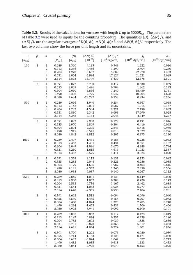
Chapter 3. Crustal pinning 35
Table 3.3: Results of the calculations for vortexes with length L up to 5000Rws. The parametersof table 3.2 were used as inputs for the counting procedure. The quantities ⟨D⟩, ⟨∆N⟩/eL and⟨∆E⟩/L are the angular averages of D(θ ,φ), ∆N(θ ,φ)/eL and ∆E(θ ,φ)/L respectively. Thelast two columns show the force per unit length and its uncertainty.
L β # rc ⟨D⟩ ⟨∆N⟩/ L ⟨∆E⟩/L fL σ fL[Rws] [Rws] [Rws] [10−2] [104 erg/cm] [1015 dyn/cm] [1015 dyn/cm]
100 1 1 0.289 1.320 4.185 0.549 1.222 0.0862 0.313 1.356 4.466 1.290 3.404 0.2503 0.204 1.270 -3.687 5.689 22.970 1.4534 0.531 2.064 -5.994 17.127 61.521 5.6895 2.514 3.893 -13.779 5.439 12.578 2.501
3 1 0.591 2.072 6.730 0.417 0.630 0.0692 0.555 2.005 6.496 0.704 1.362 0.1433 0.504 2.060 -5.866 7.240 18.459 1.7514 1.490 3.396 -9.725 5.542 10.904 1.6985 8.080 4.634 -23.797 0.553 0.994 0.256
500 1 1 0.289 2.066 1.940 0.254 0.367 0.0582 0.313 2.142 2.031 0.587 1.015 0.1673 0.204 1.732 -1.504 2.321 7.190 0.8334 0.531 2.880 -2.342 6.693 17.690 3.0285 2.514 4.348 -5.184 2.046 4.349 1.277
3 1 0.591 3.092 2.900 0.179 0.191 0.0462 0.555 2.970 2.809 0.304 0.416 0.0953 0.504 2.804 -2.305 2.845 5.418 0.9464 1.490 3.915 -3.541 2.018 3.529 0.7265 8.080 4.842 -8.812 0.205 0.375 0.130
1000 1 1 0.289 2.407 1.431 0.188 0.238 0.0532 0.313 2.467 1.491 0.431 0.651 0.1523 0.204 2.049 -1.086 1.676 4.388 0.7444 0.531 3.210 -1.615 4.616 11.033 2.5875 2.514 4.467 -3.575 1.411 3.024 1.090
3 1 0.591 3.358 2.113 0.131 0.133 0.0422 0.555 3.283 2.044 0.221 0.286 0.0883 0.504 3.129 -1.606 1.982 3.403 0.8164 1.490 4.131 -2.362 1.346 2.350 0.5665 8.080 4.938 -6.037 0.140 0.267 0.112
2500 1 1 0.289 2.845 1.031 0.135 0.149 0.0502 0.313 2.900 1.067 0.308 0.420 0.1433 0.204 2.533 -0.756 1.167 2.462 0.6884 0.531 3.544 -1.062 3.034 6.777 2.3245 2.514 4.648 -2.355 0.930 2.184 0.981
3 1 0.591 3.663 1.513 0.094 0.096 0.0402 0.555 3.530 1.455 0.158 0.207 0.0833 0.504 3.468 -1.074 1.325 2.205 0.7404 1.490 4.294 -1.463 0.833 1.506 0.4665 8.080 4.992 -3.941 0.092 0.190 0.101
5000 1 1 0.289 3.067 0.852 0.112 0.123 0.0492 0.313 3.147 0.884 0.255 0.339 0.1403 0.204 2.783 -0.603 0.930 1.828 0.6564 0.531 3.731 -0.828 2.366 5.317 2.2335 2.514 4.681 -1.834 0.724 1.801 0.936
3 1 0.591 3.799 1.223 0.076 0.080 0.0392 0.555 3.714 1.183 0.128 0.171 0.0803 0.504 3.632 -0.844 1.042 1.677 0.7134 1.490 4.482 -1.085 0.618 1.133 0.4335 8.080 5.044 -2.996 0.070 0.153 0.096

Chapter 3. Crustal pinning 36
0
5.0⋅1015
1.0⋅1016
1.5⋅1016
2.0⋅1016
2.5⋅1016
3.0⋅1016
3.5⋅1016
4.0⋅1016
0 2.0⋅1013 4.0⋅1013 6.0⋅1013 8.0⋅1013 1.0⋅1014 1.2⋅1014 1.4⋅1014
f L [
dyn
cm-1
]
ρ [g cm-3]
l = 6 Rwsl = 8 Rws
l = 10 Rwsl = 12 Rwsl = 14 Rwsl = 16 Rws
Figure 3.8: Convergence test for the l parameter used in our calculation. In this figure wecan see the pinning force per unit length for the five zones of the inner crust, obtained withdifferent choices of the parameter: increasing the value of l the curves become closer, showingthe convergence of the model. This picture corresponds to a vortex of length L = 200Rws.
matter (Gandolfi et al., 2008). The results for the pinning force per unit length arealso plotted in fig. 3.10 for β = 1 and in fig. 3.11 for β = 3. In the table we also showthe results for ⟨D⟩, for ⟨∆N⟩/eL and for ⟨∆E⟩/L, which are the angular averages ofD(θ ,φ), ∆N(θ ,φ)/eL, and ∆E(θ ,φ)/L respectively. We notice that | ⟨∆N⟩ |/eL 0.5when eL ∼ 103, which confirms the inadequacy of using symmetric vortex-latticeconfigurations when evaluating the mesoscopic pinning force (Jones, 1990b).
From these results it is possible to see that there is a strong dependence of thepinning force per unit length on the parameter L: increasing the length of the vortexa consistent decrease in the mesoscopic pinning force can be observed. This behaviorwas indeed expected, following the argument by Jones (1991b) that the difference inenergy between adjacent configurations becomes vanishingly small for infinite vortexrigidity (L →∞). However, using a realistic vortex length of order ∼ 103Rws, asdiscussed in section 3.2.3, the pinning force is still not negligible.
The other important parameter of the model is the polarization factor β . Theresults show that fL doesn’t depend very strongly on the choice of this parameter in thethree lower density regions, while the effect is more important in the two high densityregions, where the mesoscopic pinning force is significantly larger in the strong pairingscenario (β = 1) than in the weak one (β = 3). It’s also worth noting that changingthe polarization factor from β = 1 to β = 3, results in a shift to lower densities of the

Chapter 3. Crustal pinning 37
0
5.0⋅1015
1.0⋅1016
1.5⋅1016
2.0⋅1016
2.5⋅1016
3.0⋅1016
3.5⋅1016
0 2.0⋅1013 4.0⋅1013 6.0⋅1013 8.0⋅1013 1.0⋅1014 1.2⋅1014 1.4⋅1014
f L [
dyn
cm-1
]
ρ [g cm-3]
dh = 0.100 Rwsdh = 0.050 Rwsdh = 0.010 Rwsdh = 0.005 Rws
Figure 3.9: Convergence test for the dh parameter used in our calculation. As in fig. 3.8 wecan see that decreasing the value of dh the curves become closer, showing the convergence ofthe model also for this parameter. This picture corresponds to a vortex of length L = 200Rws.
maximum of the pinning profile. The position in density of the maximum pinningforce can be relevant to determine the angular momentum accumulated in the crustbetween pulsar glitches, as discussed in Pizzochero (2011).
A comparison between our results and those found in the literature shows that themaximum pinning forces per unit length obtained in this work are at least two ordersof magnitude smaller than those found for an aligned vortex (Alpar et al., 1984a;Anderson et al., 1982) and which have been commonly used in the study of pulsarglitches. As we shall discuss in the following, however, they are still large enough toaccount for the large glitches observed in the Vela pulsar.
3.4.1 Analytic approximations
The results presented up to now refer to the calculation of the mesoscopic pinning forcecorresponding to the fiducial parameters Rws, RN , ξ and Ep in table 3.1. However,existing or future calculations of the inner crust nuclear structure, of the neutronsuperfluid pairing properties and of the microscopic vortex-nucleus interaction mayprovide alternative sets of parameters to those used in the present work. It is possibleto generalize our approach and obtain a simple analytic expression which allowsto calculate the pinning force per unit length fL for different choices of the inputparameters.

Chapter 3. Crustal pinning 38
1.0⋅1013
1.0⋅1014
1.0⋅1015
1.0⋅1016
1.0⋅1017
0 2.0⋅1013 4.0⋅1013 6.0⋅1013 8.0⋅1013 1.0⋅1014 1.2⋅1014 1.4⋅1014
f L [
dyn
cm-1
]
ρ [g cm-3]
L100, β1L500, β1L1000, β1L2500, β1L5000, β1
Figure 3.10: The pinning force per unit length for the β = 1 case. The mesoscopic pinningforce is plotted as a function of the baryonic density of matter for the five zones consideredand for different vortex lengths.
In eq. (3.20), the quantity Eeff can be factorized. We can also express all thelengths in Rws units and then define an adimensional quantity ef
eL(erc) that dependsonly on the adimensional capture radius erc = rc/Rws and the adimensional vortexlength eL = L/Rws. The quantity ef
eL(erc) is purely geometrical and it contains all theinformation obtained from the counting procedure described in the preceding sections.The force per unit length fL (in dyn/cm) can then be obtained as
fL =Eeff
R2ws
efeL
rc
Rws
(3.21)
where Eeff must be expressed in MeV and the radius of the Wigner–Seitz cell in cm.We have calculated ef
eL(erc) for different choices of erc (in the realistic range 0÷ 8)and for different vortex lengths (of order eL ∼ 103) for both the NP and IP regimesWe then fitted a non-linear function f ∗(x) to the calculated values of ef
eL: we used afunction of the form
f ∗ = Ax + B [log(1+ x)]W + C (3.22)
where A, B, C and W are the parameters to be fitted. In fig. 3.12 we show the resultsfor the eL = 5000 case; the error bars have also been added, as obtained from thepropagation of the error on nNbound
(θ ,φ). We see that the calculated points can be fittedreasonably (within the error bars) with the choice of parameterization in eq. (3.22).In table 3.4 we give the parameters obtained from the fitting procedure.

Chapter 3. Crustal pinning 39
1.0⋅1013
1.0⋅1014
1.0⋅1015
1.0⋅1016
1.0⋅1017
0 2.0⋅1013 4.0⋅1013 6.0⋅1013 8.0⋅1013 1.0⋅1014 1.2⋅1014 1.4⋅1014
f L [
dyn
cm-1
]
ρ [g cm-3]
L100, β3L500, β3L1000, β3L2500, β3L5000, β3
Figure 3.11: The pinning force per unit length for the β = 3 case. The pinning force per unitlength for the β = 1 case. The mesoscopic pinning force is plotted as a function of the baryonicdensity of matter for the five zones considered and for different vortex lengths.
Table 3.4: Fit parameters for the function f ∗ = Ax + B [log(1+ x)]W + C . Three differentvortex lengths L are considered for both the NP and IP regimes.
A B W C[10−10] [10−9] [10−8]
L = 1000 Rws NP - 5.04 -2.08 1.974 -1.169IP -33.63 14.49 1.586 1.155
L = 2500 Rws NP -12.10 1.80 -0.366 -0.995IP - 5.99 12.31 0.997 0.490
L = 5000 Rws NP -10.35 0.75 -0.643 -0.726IP -12.36 12.24 1.114 0.389

Chapter 3. Crustal pinning 40
-5.0⋅10-8
-4.0⋅10-8
-3.0⋅10-8
-2.0⋅10-8
-1.0⋅10-8
0
1.0⋅10-8
2.0⋅10-8
3.0⋅10-8
4.0⋅10-8
5.0⋅10-8
0 1 2 3 4 5 6 7 8 9
IP
NP
IP
NP
IP
NP
f*
rc [Rws]
Figure 3.12: Plot of the calculated values of efeL (for eL = 5000) as a function of the capture
radius rc (in units of Rws). The error bars for the estimated errors on efeL are also shown. The
squares are the values of efeL corresponding to the ten values of rc in table 3.2. The fitting
curves f ∗ for both the interstitial (above) and nuclear (below) pinning regimes are also shown(see table 3.4).
We notice that, within the uncertainty given by the quite large error bars, there is nosignificant difference in the magnitude of ef
eL(erc) between the nuclear and the interstitialregime. This means that the force per unit length, for given erc and Eeff, remains roughlythe same if we take the microscopic vortex-nucleus force to be attractive or repulsive.The fact that attractive and repulsive vortex-nucleus interactions are equivalent forthe pinning of vortexes to the lattice was already noted by Link (2009).
3.5 Conclusions
In this chapter we have presented a realistic calculation of the pinning force per unitlength acting on a vortex in a neutron star crust. We have calculated the mesoscopicpinning force at different densities for straight vortexes that cross the star inner crust,and averaged over all the possible orientations of the crustal lattice with respect tothe vortex. Our results confirm the expectations of (Jones, 1991b), that the averagingprocedure over different orientations tends to smooth out energy differences betweendifferent configurations, leading to weaker pinning forces. In the limit of infinitelylong vortexes the pinning force would vanish; for realistic values of the vortex tension

Chapter 3. Crustal pinning 41
the force per unit length is, however, still sizable and in the range fL ≈ 1014 − 1015
erg/cm depending on the position in the crust. We find that the mesoscopic pinningforce depends very little on whether the pinning force is attractive (nuclear pinning) orrepulsive (interstitial pinning) in a given region of the star, but it can be quite sensitiveto in-medium polarization effects, which can shift the position of the maximum andthus alter the angular momentum distribution in the crust of a neutron star.
In the following chapter we will apply the calculated forces to the problem ofpulsar glitches in order to understand if these results can explain large glitches in theVela pulsar, within the framework of the “snowplow” model (Pizzochero, 2011). Moregenerally the forces that we have calculated can be used to generate realistic pinningprofiles for glitch models (Haskell et al., 2012c; Haskell and Antonopoulou, 2013),simulations of vortex dynamics in neutron stars (Warszawski and Melatos, 2008) ormode calculations (Glampedakis and Andersson, 2009; Link, 2012a).

CHAPTER 4Core pinning
The pinning interaction in the core of a neutron star is a much less explored problemthan the crustal pinning one faced in chapter 3. In the NS interiors, matter is not orga-nized in lattice because it’s in superfluid and superconductive state: an hypotheticalpinning force can’t be related to vortex–lattice interaction. Instead it’s possible, undercertain circumstances, an interaction of the vortex with the magnetic flux carried bythe superconductive protons. Currently it’s yet unclear if protons in the core form atype I superconductor, in which the magnetic field is contained in regions of normalprotons (Sedrakian, 2005) and therefore pinning effects are excluded (Jones, 2006),or they make a transition to a type II superconductivity state (Migdal, 1959; Baymet al., 1969). In this latter case the magnetic flux is confined to flux tubes and apinning interaction between vortexes and flux tubes is possible. The transition fromtype II to type I occurs above a critical density that is expected to be bigger thanthe nuclear saturation density but it’s still unknown, due to the uncertainties in thenucleon–nucleon potentials (Link, 2003).
In the following chapters we will face the problem from a macroscopic point ofview: we will test the “snowplow” model firstly without any form of pinning in theneutron star interiors, and after, in chapter 6, considering that a fraction of the vorticityin the core is completely blocked by entanglement with the flux tubes. Conversely inthis chapter we want to adopt a mesoscopic approach, applying the same conceptualideas of chapter 3 to estimate the pinning force per unit length in the core of a neutronstar. We will show that the core pinning (if the star is actually in type II state) is twoorders of magnitude lower than the crustal one, and this means that, according to theresults of chapter 6, it can be safely neglected in our macroscopic glitch model.
4.1 A simple approach
In type II superconductor core of a neutron star, the magnetic flux is confined insidetubes that have a core of normal protons; the radius of this region can be taken equalsto the proton coherence length ξp ≈ 10 fm. On the other side the coherence length
42

Chapter 4. Core pinning 43
for neutrons, and therefore the radius of the vortex, is ξn ≈ 25 fm (Link, 2003). Thecoupling between the two condensates is due to the induced proton current around thevortexes that magnetizes them (Alpar et al., 1984c; Chau et al., 1992; Harvey et al.,1986): this kind of entrainment generate the pinning force because a magnetizedneutron vortex interact with the flux confined in the tubes. Outside the flux tube,the magnetic field falls off exponentially over a distance equal to the London length.We identify this quantity with Λp that is approximately equals to 80 fm, and in thesame way we call Λn ≈ 10 fm the length scale over which the magnetic field of thevortex decays. Results of Ruderman et al. (1998); Link (2003, 2012a) indicate thatthe energy increase per single interaction between a vortex approaching a flux tube isEp ≈ 5MeV, over the length range Λp.
To calculate the pinning force per unit length in the core we can use a very simplemodel, as done by Link (2003). We can consider a straight vortex immersed in anarray of flux tubes. These tubes form a two dimensional quadratic array in the x yplane and they extend in the z direction. The vortex lies in the x y plane, alignedwith a versor of the lattice and therefore perpendicular to the flux tubes. Given thatthe force per single interaction is Fp = Ep/Λp, the force per unit length can be easilyevaluated as
f =Fp
lφ=
Ep
Λp lφ, (4.1)
where lφ is the average spacing between flux tubes. This quantity depends on themagnetic field B of the star because lφ = 1/
p
nφ, where nφ = B/Φ0 (Φ0 = πħhc/eis the flux quantum). We can express B in unit of 1012 G (we identify this quantityas B12, and we will use the realistic value of ≈ 1 in the following; for a magnetarB12 ≈ 100÷ 1000, as we’ll discuss) obtaining the benchmark lφ ≈ 3000/
p
B12fm. Asa conclusion, the approach here described gives as result an order of magnitude forthe core pinning force per unit length of 1015 dyn/cm (see Link (2003)).
4.2 The realistic mesoscopic model
The naive calculation just described here gives as result the maximum pinning forcebecause it considers only the aligned configuration. Qualitatively this is the sameapproach of the first works about the crustal pinning, that were focused on the forceper single interaction Fp; then the force per unit length was simply found by dividingthis quantity by the spacing between pinning site. In chapter 3 we overcome thisschema, justifying the need to consider and average all possible orientations betweenvortex and the lattice. Here we are focusing on the core pinning due to the vortex–fluxtube interaction that is quite different under some physical points of view, butwe can apply the same conceptual approach (that we review here) of the previouschapter to correctly estimate the force per unit length fp. In fact the vortex has a finiterigidity and this means that can be considered straight only on a length scale L; onlarger scale the interaction with fluxtubes will bend the vortex, changing its orientation

Chapter 4. Core pinning 44
Figure 4.1: Schematic representation of avortex immersed in a regular lattice of flux–tubes, all oriented in the same direction.
with the lattice. Moreover, unlike the vortexes that are expected to be approximatelyparallel to the rotational axis of the star (except for bending), the flux tube arrayhas a complicated structure because the tubes are twisted and therefore entanglethe vortexes. The geometric configuration that we take into account is described infig. 4.1. We consider a vortex of finite length immersed in a lattice of straight fluxtubeswith a generic casual orientation. The tubes extend parallel over the z direction andare infinitely long; in the x y plane they are equally spaced on a regular grid. TheWigner–Seitz radius of the lattice cell is Rws and of course the distance between twoconsecutive tubes in the grid is 2 Rws. As discussed before, Rws = lφ/2 and thereforeits value depends on the magnetic field of the star by the following relation:
Rws =1500p
B12fm. (4.2)
It’s important to note that here, by the moment, we don’t take into account the twistedstructure of the fluxtubes (for the entanglement effect), as this aspect will be coveredlater. To estimate the length L on which the vortex can be considered rigid, we can usethe same technique of section 3.2.3: the eq. (3.15) indicates that L, in units of Rws,scales as ∼ 2TRws/Ep where T is the tension of the vortex. Even if we use the sametension used in section 3.2.3 for crustal pinning, the results in this case will be differentbecause Rws, that control the scale of the problem, is bigger. In fact, following theprescription used by Link (2003), Rws ≈ 1500 fm (in the crustal pinning this parameteris ∼ 30 fm), and this lead certainly to L ∼ 104 Rws. As we will show later, a longervortex will results, as expected, in a lower pinning force per unit length f . We’llsee that even just taking L = 1000 Rws, f will be at least two orders of magnitudelower that the crustal pinning case (enough to justifying the neglect in the snowplowmodel). Iin order to maintain the computational time affordable, we will perform ourcalculations here with these four different choices of L: 1000 Rws, 2500 Rws, 5000 Rwsand 10000 Rws.

Chapter 4. Core pinning 45
Figure 4.2: Number of captured pinning sites N(λ,κ) when the vortex is aligned with thelattice. The color codes are described in the sidebar. The axes κ and λ represent the translationof the vortex with respect to the initial position, and they are measured in Rws units. Thegrid step size is dh = 0.01 Rws, the vortex length is L = 500 Rws and the capture radius isrc = 0.027 Rws. The lattice is the one represented in fig. 4.1
To explain the algorithm used, let’s start with a vortex with a random orientationwith respect the fluxtubes array. The orientation is identified using standard polarcoordinates, therefore with the angles θ and φ that the vortex form with the lattice.For a given choice of (θ ,φ), we perform a counting procedure by moving the vortexparallel to itself, covering a square region with side l, with steps of an amount dh. Weidentify the displacement of the vortex from the initial position with (λ,κ), and foreach new position we count the number of intersections N(λ,κ) that the vortex haswith the tubes.
This problem becomes simpler (and is geometrically equivalent) if we considerthe fluxtube as a line without dimension, while the vortex is a cylinder with a captureradius rc = ξp+ξn. This means that every time a “flux–line” falls into the cylinder thatrepresent the neutron vortex we must increment our counter. The fig. 4.2 shows withcolor codes the number of interaction as a function of the position (λ,κ). This plotsrepresents the extreme case when the vortex is perfectly aligned with the fluxtubes array,namely θ = φ = 0: as expected a single interaction is recorded only at correspondenceof a tube, creating a regular simple pattern. The coordinates λ and κ are given inRwsunits and the dark dots are so small because the capture radius is tiny comparedto the spacing between tubes: the benchmarks by Link (2003) in fact indicate that

Chapter 4. Core pinning 46
Figure 4.3: Number of captured pinning sites N(λ,κ) when the vortex is non–aligned withthe lattice (we selected a random orientation). The color codes are described in the sidebar.For details on the parameters used to produce this plot see fig. 4.2
rc ∼ 0.025 Rws. On the other hand, fig. 4.3 shows a more general situation, in whichthe vortex is randomly aligned with the lattice: we can see an alternation of light anddark lines that represent zones where the number of interactions reaches its minimumand maximum value respectively.
The single vortex–fluxtube interaction can be repulsive (R) or attractive (A) de-pending on whether the magnetic fields are aligned or antialigned: this fact reflects ina different sign of the quantity Ep that can be positive (R case) or negative (A case).We must cover these two cases separately, in order to correctly evaluate the pinningforce per unit length. In the attractive regime, we identify the bound positions withthe displacements (λ,κ) of the vortex for which the number of interactions is maximal,i.e. N(λ,κ) = Nbound =max(N(λ,κ)). On the contrary, the repulsive situation focuseson the minimum number of interaction (this defines the bound positions), and thismeans that Nbound =min(N(λ,κ)).
Once we have dealt this distinction, we can properly calculate the force with ageneralized approach that covers both cases. In fact the change in energy obtained bymoving the vortex away from its bound configuration will be:
∆E(θ ,φ) = Ep(Nfree(θ ,φ)− Nbound(θ ,φ)) (4.3)
where we take Nfree as the average number of interactions counted in all visiteddisplacements: Nfree(θ ,φ) = ⟨N(λ,κ)⟩. The force (per unit length) required to move

Chapter 4. Core pinning 47
away the vortex from the bound position is therefore easily calculated as
fL(θ ,φ) =∆E(θ ,φ)L D(θ ,φ)
, (4.4)
where D(θ ,φ) is the average distance between the bound and free configuration.Until now, the procedure described is the same one that has been applied also for
the pinning in the inner crust of the neutron star. The calculation of the mean distanceD(θ ,φ) is however a little different. In chapter 3 we have used the surface density ofthe bound configurations, but here the pattern showed in fig. 4.3 suggests anotherapproach. The degeneration of the lattice in the z direction reflects in density plotwith alternating “vertical” stripes of positions with equal energy. The fact that thesestripes are oriented vertically depends on our choice of the reference system for (λ,κ);with a different choice the stripes would be oblique, but the model remains valid andconsistent. Therefore we count the number nNbound
of disjoint line–like regions forwhich the number of intersection is Nbound and use the linear density of these, i.e:
D(θ ,φ) =l
nNbound(θ ,φ)
, (4.5)
where l is the side of the square region covered with the parallel transport procedure.The last step of our algorithm is averaging over all possible orientation, thus performingan integration over the whole solid angle dΩ= sinθ dθ dφ.
As described before, a single interaction affects the energy of the configurationby a fixed amount Ep, no matter at what angle, between vortex and fluxtube, theintersection occurs. A better approach could be considering the intersecting volume,but unfortunately this picture would be computationally intractable. A reasonablesolution can be found by following the idea that this intersecting volume leads to afactor 1/ sinθ that must be included in the calculations. We can therefore define anew quantity Eeff which is the effective energy per interaction and has the followingexpression:
Eeff = Ep| cosθ |sinθ
(4.6)
The factor | cosθ | in this equation cames from the expression of the magnetic energybetween two dipole. The final equation for the pinning force per unit length is then:
fL =1
4πEp
∫
Nfree(θ ,φ)− Nbound(θ ,φ)L D(θ ,φ)
| cosθ |sinθ
dΩ. (4.7)
4.2.1 Flux–tubes entanglement
Until now we have considered straight flux tubes that are parallel to the z axis andtherefore they form a regular oriented array. Anyway, as pointed out by Rudermanet al. (1998); Link (2003) this array has likely a much more complicated structurebecause the flux tubes are twisted and entangled. Of course this effect can impact

Chapter 4. Core pinning 48
Figure 4.4: Schematic representation of avortex immersed in the lattice used to modelthe entanglement. We can see the differentplanes of parallel fluxtubes.
over the results of our model and we want now to take into account this aspect. Inorder to accomplish this requirement, we change the lattice structure by consideringalternating planes of tubes perpendicular to the y direction. Each plane containsparallel tubes oriented with an angle α relative to the z direction. The sequence ofthe angles α is 0,−π/4, 0,π/4, 0,−π/4, . . . . This configuration, showed in fig. 4.4,permits us to model the entanglement, maintaining a net magnetic field oriented asthe z direction. The spacing between these planes is the same of the spacing betweenthe flux–tubes in one plane, i.e. 2 Rws: this guarantees that the distance between twotubes is always greater than this value.
With this new configuration we can apply the same counting procedure, by movinga randomly oriented vortex with a parallel transport operation. The typical densityplot is different from the case without entanglement, because the alternate planesof tubes brake the degeneracy showed in fig. 4.3. The plot of fig. 4.5 represent thesituation of a randomly oriented vortex when the entanglement is taken into account.The details of the model described until now remains valid except for eq. (4.5) whichspecifies our definition of the average distance between the bound configuration, andmust be corrected. We adopt the same approach used for the crustal pinning (seeeq. (3.18) in chapter 3), as the typical patterns in the density plots are similar. Thenumber nNbound
, in this case, is therefore the number of disjoint regions for whichthe number of intersection between the vortex and the flux–tubes is Nbound. In thiscontext we consider two points spaced by less that η= 2ξp as belonging to the samedisjoint region, for the reasons treated in chapter 3 (we will discuss mode deeply aboutthe parameter η in the following section). The average spacing between extremalconditions is
D(θ ,φ) =l
Æ
πnNbound(θ ,φ)
(4.8)
as they are uniformly distributed in the (λ,κ) plane. The expression for the force per

Chapter 4. Core pinning 49
Figure 4.5: Number of captured pinning sites N(λ,κ) when the vortex is non–aligned withthe lattice (we selected a random orientation) when the entanglement is considered. The colorcodes are described in the sidebar. For details on the other parameters used to produce thisplot see fig. 4.2.
unit length of a single orientation remain identical to eq. (4.4), and the average overthe whole solid angle leads to the final result:
fL =1
4πEp
∫
Nfree(θ ,φ)− Nbound(θ ,φ)L D(θ ,φ)
| cosθ |sinθ
dΩ. (4.9)
4.3 Results
In eq. (4.7) we can see that Ep is factorized and, from the discussion of the previoussection, we know that all the counted quantities depend only on the capture radius rc .A specific discussion must be done for the disjoint parameter η because this quantityapparently doesn’t depends on rc, as we take it to be η = 2ξp. Anyway it’s easy toshow that this is not true. In fact, the neutron and proton coherence lengths can beexpressed in the following way (Mendell, 1991):
ξp ≈ 16 x1/3p ρ
1/314 ∆p(MeV)−1fm (4.10)
ξn ≈ 16 x1/3n ρ
1/314 ∆n(MeV)−1fm (4.11)

Chapter 4. Core pinning 50
where we have neglected the entrainment in the core; moreover xp and xn representrespectively the proton and neutron fraction over the total density andρ14 is the densityexpressed in 1014 g cm−3 units. By taking the realistic benchmarks ∆n =∆p = 1 MeV,xn = 0.95, xp = 0.05 and ρ14 = 2.8 we obtain ξp ≈ 8.5 fm and ξn ≈ 22 fm. The
expressions provided indicate also that (ξp/ξn) '
xp/xn
1/3and therefore we can
express the capture radius as
rc = ξp + ξn =
1+
xn
xp
1/3
ξp (4.12)
and then, as we take η= 2ξp, we have
η=2
1+
xnxp
1/3rc (4.13)
With realistic values for the proton and neutron fractions in the core of a neutron starwe obtain η' 0.55rc . We can thus express all the lengths in Rwsunits (for this purposewe will write eL to indicate L/Rws) and define a new quantity ef
eL that depends only onthe parameter erc = rc/Rws. Then the force per unit length fL (in dyn cm−1) can beobtained as fL = ef
eL(erc)Ep/R2ws, where Ep must be expressed in MeV and the radius of
the Wigner–Seitz cell in cm.In the following, the pinning force per unit length will be given thus as ef
eL becausethis generalized version gives the possibility of calculating the result for specificvalues of Ep and Rws. Of course the dependence of ef
eL on the vortex length L can’tbe removed, therefore the four cases indicated will be explored, namely 1000 Rws,2500 Rws, 5000 Rws and 10 000 Rws. The calculations rely on the appropriate choiceof the parameter l (side of the square region considered during the parallel–transportoperation) and of the grid step dh. In fig. 4.6 we show the convergence of our results forl and dh. The first parameter affects the calculation of the factor D because increasingl reflects in a more accurate evaluation of the density of maximal position: covering asquare region of side l = 16 Rws (as done in the following) is enough to count a goodvalue of bound sites, from the statistical point of view. In the meanwhile a tiny gridstep dh= 0.005 Rws is required to resolve all the bound positions, for the smallnessof the capture radii used. A further reduction of this parameter wouldn’t change theresult thanks to the fact that we consider only the disjoint regions, regardless of howdensely they are sampled.
The figs. 4.7 to 4.9 show our calculations with the parameters indicated, fordifferent vortex lengths. We cover both the attractive case (A, negative values ofthe force) and the repulsive one (R) by evaluating the pinning force per unit lengthefeL as a function of the capture radius rc: the dots in the plots correspond to the
configurations considered. Every case is explored with the two lattice types, to coverboth the non–entangled and the entangled condition. The confidence levels of 1σare also plotted: given that we are dealing with a counting procedure, we can simply

Chapter 4. Core pinning 51
1.6⋅10-8
1.8⋅10-8
2.0⋅10-8
2.2⋅10-8
2.4⋅10-8
2.6⋅10-8
2.8⋅10-8
3.0⋅10-8
3.2⋅10-8
1.0⋅10-2 1.5⋅10-2 2.0⋅10-2 2.5⋅10-2 3.0⋅10-2 3.5⋅10-2
f*
rc [Rws]
dh = 0.100 Rwsdh = 0.050 Rwsdh = 0.010 Rwsdh = 0.005 Rws
1.6⋅10-8
1.8⋅10-8
2.0⋅10-8
2.2⋅10-8
2.4⋅10-8
2.6⋅10-8
2.8⋅10-8
3.0⋅10-8
3.2⋅10-8
f*
l = 4 Rwsl = 6 Rwsl = 8 Rwsl = 10 Rws
Figure 4.6: Convergence test for the parameters l and dh used in our calculation. In thisfigure we can see the pinning force per unit length ef
eL for different values of the capture radiusrc: increasing the value of l the curves become closer, showing the convergence of the model.An analogous effect is obtained by reducing the step size dh in the parallel transport operation.These pictures correspond to a vortex of length L = 5000 Rws.
assume that the result of our integration for a single orientation is nNbound±pnNbound
.We can then propagate this error in eqs. (4.4) and (4.7) to obtain the required resultefeL ±σef
eL. The explored range for the capture radius is (5× 10⁻³÷0.7)Rws: this choice
is driven to the fact that for a magnetar rc/Rws is much bigger than in a normal pulsar.In this work we consider rc = 30 fm for both cases, but of course the magnetic field ineq. (4.2) change significantly from B12 = 1 for a pulsar (and therefore rc = 0.02 Rws)to B12 = 1000 (which corresponds to rc = 0.6 Rws) for a magnetar.
The curves in these plots are the results of a fitting procedure that provides ananalytic expression for the quantity ef
eL(rc). We fit a non-linear function f (x) to thecalculated values of ef
eL for different choices of rc/Rws: the function used is
f ∗ = Ax + B [log(1+ x)]W + C (4.14)

Chapter 4. Core pinning 52
-1.0⋅10-7
-8.0⋅10-8
-6.0⋅10-8
-4.0⋅10-8
-2.0⋅10-8
0
2.0⋅10-8
4.0⋅10-8
6.0⋅10-8
8.0⋅10-8
1.0⋅10-7
0 0.1 0.2 0.3 0.4 0.5 0.6 0.7
(R)
(A)
f*
rc [Rws]
No Entranglement
0 0.1 0.2 0.3 0.4 0.5 0.6 0.7
(R)
(A)
rc [Rws]
With Entranglement
Figure 4.7: Plot of the calculated values of efeL (for eL = 1000) as a function of the capture
radius rc (in units of Rws). The error bars for the estimated errors on efeL are also shown. The
left picture refers to the simple regular lattice of flux–tubes, while on the right we have takeninto account also the entanglement by using the described lattice. The fitting curves f ∗ forboth the repulsive (above) and attractive (below) regimes are also shown (see table 4.1). Thesquares indicate the inferred values for a typical neutron star, while the triangles are referredto the capture radius for a magnetar (see text for details).
where A, B, C and W are the parameters of the fit and x is the fit variable, whichdescribes the capture radius in Rws units. The table 4.1 reports the obtained valueswhich describe the curves. All the curves are finally plotted together in fig. 4.11 forthe non–entangled case, and in fig. 4.12 for the entangled one. As expected, a longervortex is related to a smaller pinning force per unit length. It’s also worth notingthat there is no significant difference in the order of magnitude of the result fromthe attractive configuration to the repulsive one. This means that the force per unitlength, for a given capture radius, remain roughly the same if we consider the singlesite interaction attractive or repulsive. Moreover we note that there is no significantdifference in the order of magnitude between the two lattice configurations (with orwithout the entanglement) taken into account: the following considerations about theimpact of these result on pulsar glitch models are valid for both cases.

Chapter 4. Core pinning 53
-6.0⋅10-8
-4.0⋅10-8
-2.0⋅10-8
0
2.0⋅10-8
4.0⋅10-8
6.0⋅10-8
0 0.1 0.2 0.3 0.4 0.5 0.6 0.7
(R)
(A)
f*
rc [Rws]
No Entranglement
0 0.1 0.2 0.3 0.4 0.5 0.6 0.7
(R)
(A)
rc [Rws]
With Entranglement
Figure 4.8: Plot of the calculated values of efeL (for eL = 2500) as a function of the capture
radius rc (in units of Rws). See fig. 4.7 for other details.
-4.0⋅10-8
-3.0⋅10-8
-2.0⋅10-8
-1.0⋅10-8
0
1.0⋅10-8
2.0⋅10-8
3.0⋅10-8
4.0⋅10-8
0 0.1 0.2 0.3 0.4 0.5 0.6 0.7
(R)
(A)
f*
rc [Rws]
No Entranglement
0 0.1 0.2 0.3 0.4 0.5 0.6 0.7
(R)
(A)
rc [Rws]
With Entranglement
Figure 4.9: Plot of the calculated values of efeL (for eL = 5000) as a function of the capture
radius rc (in units of Rws). See fig. 4.7 for other details.

Chapter 4. Core pinning 54
-4.0⋅10-8
-3.0⋅10-8
-2.0⋅10-8
-1.0⋅10-8
0
1.0⋅10-8
2.0⋅10-8
3.0⋅10-8
4.0⋅10-8
0 0.1 0.2 0.3 0.4 0.5 0.6 0.7
(R)
(A)
f*
rc [Rws]
No Entranglement
0 0.1 0.2 0.3 0.4 0.5 0.6 0.7
(R)
(A)
rc [Rws]
With Entranglement
Figure 4.10: Plot of the calculated values of efeL (for eL = 10000) as a function of the capture
radius rc (in units of Rws). See fig. 4.7 for other details.
-4.0⋅10-8
-3.0⋅10-8
-2.0⋅10-8
-1.0⋅10-8
0
1.0⋅10-8
2.0⋅10-8
3.0⋅10-8
4.0⋅10-8
0 0.1 0.2 0.3 0.4 0.5 0.6 0.7
(R)
(A)
f*
rc [Rws]
L=1000L=2500L=5000
L=10000
Figure 4.11: Plot of the fitting curves of table 4.1 obtained with the simple lattice withoutconsidering the entanglement effect.

Chapter 4. Core pinning 55
Table 4.1: Fit parameters for the function f ∗ = Ax+B [log(1+ x)]W +C . Four different vortexlengths L are considered for both the attractive (A) and repulsive (R) regimes. We give theresults also for the entangled configurations.
A B W C[10−7] [10−6] [10−8]
No
Enta
ngle
men
t
L = 1000 Rws A 6.546 −0.986 1.325 −3.610R −11.230 1.695 1.296 4.814
L = 2500 Rws A 2.667 −0.396 1.319 −1.778R −4.044 0.611 1.301 2.328
L = 5000 Rws A 1.496 −0.218 1.297 −1.128R −1.818 0.274 1.297 1.473
L = 10 000 Rws A 0.865 −0.119 1.252 −0.798R −0.803 0.121 1.293 1.083
Wit
hEn
tang
lem
ent L = 1000 Rws A 9.315 −1.403 1.328 −6.051
R −21.590 3.253 1.289 8.503L = 2500 Rws A 3.924 −0.585 1.330 −3.198
R −8.319 1.249 1.284 3.681L = 5000 Rws A 2.214 −0.328 1.335 −2.194
R −3.137 0.470 1.285 1.912L = 10 000 Rws A 0.981 −0.141 1.348 −1.542
R −0.770 0.113 1.295 1.087
4.4 Conclusions
The results presented here are given in such way that they don’t depend on theparticular value of the Wigner–Sietz cell radius and of the single interaction energy:they are valid over a large range for the capture radius rc and can be specialized whenneeded. However it’s interesting to estimate the force, using the benchmarks presentedpreviously (see also Link (2003)) that are so far the most realistic indication for thevalues of Ep, Rws and rc in the core of a neutron star. These results are reported inthe upper part of table 4.2. Similarly we evaluate the same quantities for a magnetar(lower part of the table), for which we take a different capture radius, as describedbefore. With regard to the values related to the pulsar case, they are significantlylower (more than two orders of magnitude) that the ones obtained with analoguetechnique of the crustal pinning (see chapter 3): this justify the assumption used inthe snowplow model (see chapter 5) where we consider that the part of a vortex whichthreads the core of the neutron star is not subjected to a pinning–like interaction.
Anyway, a comparison of these results with the ones obtained for the crust canreveal an interesting aspect of the mesoscopic pinning force. In both cases we haveseen that the geometric factor ef
eL (which depends only on the structure of the lattice

Chapter 4. Core pinning 56
-8.0⋅10-8
-6.0⋅10-8
-4.0⋅10-8
-2.0⋅10-8
0
2.0⋅10-8
4.0⋅10-8
6.0⋅10-8
8.0⋅10-8
0 0.1 0.2 0.3 0.4 0.5 0.6 0.7
(R)
(A)
f*
rc [Rws]
L=1000L=2500L=5000
L=10000
Figure 4.12: Plot of the fitting curves of table 4.1 obtained with the lattice constructed to takeinto account the entanglement effect.
and doesn’t contain any scale parameter) has always the same order of magnitudeof ≈ 10−8 dyn cm MeV−1 ≈ 0.006, regardless of the type of lattice used. This meansthat the pinning force per unit length is overall dependent on the term Ep/R
2ws; in
other words, as the pinning energy per site Ep is nearly the same in all configurations,the differences in the final results for the pinning in the crust and core (both withand without entanglement) must be addressed to the different scale factor Rws whichdescribes the spacing between the lattice sites.

Chapter 4. Core pinning 57
Table 4.2: In this table we specialize the results of the fitting procedure of table 4.1 for thetypical benchmarks of a pulsar and a magnetar.
rc Ep Rws A/R L fL fL[fm] [MeV] [fm] [Rws] [1012 dyn/cm] [1012 dyn/cm]
No Ent. With Ent.
Puls
ar
30 5 1500 A 1000 6.323 11.0152500 3.263 6.0685000 2.142 4.279
10000 1.583 3.149
30 5 1500 R 1000 8.043 13.9012500 4.200 6.2885000 2.840 3.529
10000 2.219 2.229
Mag
neta
r
30 5 50 A 1000 1139.737 3294.4712500 818.247 2152.9455000 666.678 1747.798
10000 459.340 1479.343
30 5 50 R 1000 2330.755 3674.2382500 1863.837 2274.8515000 1705.225 1754.075
10000 1628.853 1452.359

PART II
THE SNOWPLOW MODEL
CHAPTER 5The “snowplow” model
In this chapter we present the snowplow model, a fully consistent model that canexplain the large glitches (∆ν/ν≈ 10−6−10−5) recorded in a subset of pulsars knownas giant glitchers. This model has been proposed by Pizzochero (2011) and appliedanalytically to describe the average properties of giant glitchers such as the inter-glitchwaiting time, the step in frequency and that in frequency derivative. The model hasbeen initially developed in Newtonian gravity and for a polytropic equation of state, buthere we want to we extend the model to realistic backgrounds, obtained by integratingthe relativistic equations of stellar structure and using physically motivated equationsof state to describe matter in the neutron star. Especially the pinning forces used is ofthe orders of magnitude suggested by the calculations shown in the previous chapters,i.e. ∼ 1015 dyn cm−1.
We find that this more detailed treatment still reproduces the main features ofgiant glitches in the Vela pulsar and allows us to set constraints on the equation ofstate. In particular we find that stiffer equations of state are favoured and that it isunlikely that the Vela pulsar has a high mass (larger than M ≈ 1.5 M).
5.1 Pinning and vorticity
One of the most important ingredients of the model is clearly fpin(ρ), the pinning forceper unit length that acts on the vortex line as a result of its interaction with the lattice(in the inner crust). As shown in the previous chapters, although the pinning forceper pinning site can readily be evaluated from the knowledge of the pinning energy(Alpar, 1977; Epstein and Baym, 1992; Donati and Pizzochero, 2003, 2004, 2006),the force per unit length of a vortex, which is the quantity that must be equated to theMagnus force in order to understand whether a vortex is pinned or free, is much morecomplex to evaluate, as it depends on the rigidity of a vortex and on its orientationwith respect to the crustal lattice. In chapter 3 we have have performed numericalsimulations to evaluate this quantity, taking into account different orientation of thebcc lattice. We have found that the order of magnitude of the maximum pinning force
59
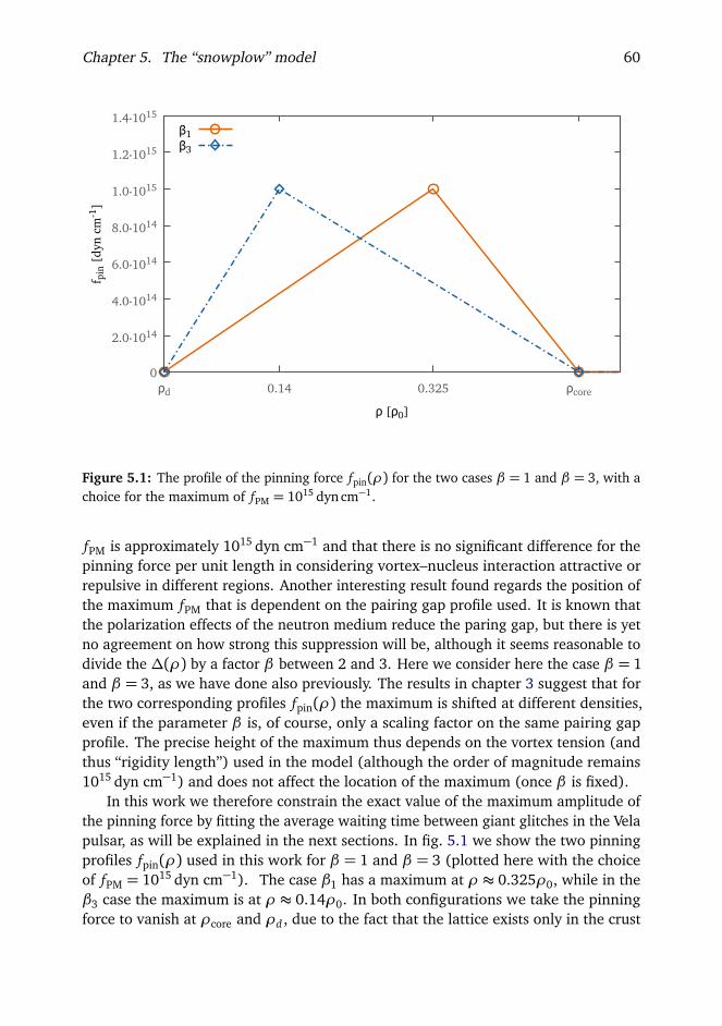
Chapter 5. The “snowplow” model 60
0
2.0⋅1014
4.0⋅1014
6.0⋅1014
8.0⋅1014
1.0⋅1015
1.2⋅1015
1.4⋅1015
ρd 0.14 0.325 ρcore
f pin
[dy
n cm
-1]
ρ [ρ0]
β1 β3
Figure 5.1: The profile of the pinning force fpin(ρ) for the two cases β = 1 and β = 3, with achoice for the maximum of fPM = 1015 dyn cm−1.
fPM is approximately 1015 dyn cm−1 and that there is no significant difference for thepinning force per unit length in considering vortex–nucleus interaction attractive orrepulsive in different regions. Another interesting result found regards the position ofthe maximum fPM that is dependent on the pairing gap profile used. It is known thatthe polarization effects of the neutron medium reduce the paring gap, but there is yetno agreement on how strong this suppression will be, although it seems reasonable todivide the ∆(ρ) by a factor β between 2 and 3. Here we consider here the case β = 1and β = 3, as we have done also previously. The results in chapter 3 suggest that forthe two corresponding profiles fpin(ρ) the maximum is shifted at different densities,even if the parameter β is, of course, only a scaling factor on the same pairing gapprofile. The precise height of the maximum thus depends on the vortex tension (andthus “rigidity length”) used in the model (although the order of magnitude remains1015 dyn cm−1) and does not affect the location of the maximum (once β is fixed).
In this work we therefore constrain the exact value of the maximum amplitude ofthe pinning force by fitting the average waiting time between giant glitches in the Velapulsar, as will be explained in the next sections. In fig. 5.1 we show the two pinningprofiles fpin(ρ) used in this work for β = 1 and β = 3 (plotted here with the choiceof fPM = 1015 dyn cm−1). The case β1 has a maximum at ρ ≈ 0.325ρ0, while in theβ3 case the maximum is at ρ ≈ 0.14ρ0. In both configurations we take the pinningforce to vanish at ρcore and ρd , due to the fact that the lattice exists only in the crust

Chapter 5. The “snowplow” model 61
weakpinningregion
strongpinningregion
cylindrical radiusRc Ric
Figure 5.2: A schematic representation ofthe geometry of our problem (out of scale).The whole shaded area represents the innercrust of the NS, where vortexes are pinnedto the lattice. The darker part indicates thestrong pinning region, where the vortexes aresubjected to pinning for their whole length.The star is threaded by straight continuousvortexes.
and that in the outer crust there are no free neutrons to produce vortexes. In thischapter we neglect any kind of pinning interaction in the core of the neutron stars:the results in chapter 4 supports this approach; anyway we will discuss this possibilityin the following chapter.
A single vortex line will be described parallel to the rotational axis and distantfrom this axis by a distance x , that represent the cylindrical radius. We consider alsothe vortex line to be continuous throughout the core: there is, in fact, no theoreticalevidence for the existence of an interface of normal matter between the core and theinner crust, that can justify the hypothesis of a core with vorticity separated from thecrust (Zhou et al., 2004). Naturally the vortexes may not be straight and parallel tothe rotational axis, as turbulence may develop in the stellar interior, especially in thepresence of strong pinning (Link, 2012a,b). We will not consider this possibility here,but will discuss some of its likely consequences in the following.
With the above hypothesis, we can identify two (cylindrical) pinning regions basedon the strength of the pinning interaction. The strong pinning region is defined byx > Rc and corresponds to the part of the star in which the vortexes lie entirely in theinner crust region, and are therefore subject to pinning for their whole length. On theother hand, in the weak pinning region (x < Rc), a vortex line is pinned only at itsextremities that are immersed in the crust, while there is no pinning interaction in thecore (see fig. 5.2).

Chapter 5. The “snowplow” model 62
5.2 The model
Thanks to the axial symmetry of the problem, we can describe the macroscopic quanti-ties of the rotating superfluid in terms of the variable n(x) that represents the numberof vortexes per unit area, at a distance x from the rotational axis of the star. Theangular velocity Ωs(x) of the superfluid component of the star is in fact proportionalto the number N(x) of vortexes enclosed in a cylindrical region of cylindrical radius x ,and can be expressed as:
Ωs(x) =κ
2πN(x)
x2=
κ
2πx2
∫
xn(x ′) da′ (5.1)
where the integration is performed on the area enclosed by the radius x . This resultfollows from the quantization of the circulation per vortex line that is encoded in theconstant κ= πħh/mN .
Once a star has been fixed by the choice of an EoS and the integration of the TOVequations, the model requires, as a first step, the evaluation of the pinning force for thewhole length of a generic vortex line. This can be obtained starting from the functionfpin(ρ) discussed previously. Let us imagine a vortex line parallel to the rotational axisof the star and distant x: the total pinning acting on it is given by the integration offpin(ρ) over its length:
Fpin(x) = 2
∫ `(x)/2
0
fpin
ρp
x2 + z2
dz (5.2)
where `(x) = 2q
R2ic − x2 is the length of the vortex line, obtained considering that
the vortex line ends at the inner–outer crust surface. To understand better the role ofthe pinning force, we choose a neutron star of 1.4 M with SLy equation of state andwe plot the function Fpin(x) for x from 0 to Ric (fig. 5.3, corresponding to β = 1 andfPM = 1015 dyn cm−1).
The pinning interaction is not the only force that acts on a vortex line. As shown inRuderman and Sutherland (1974), pinning prevents the vortex line from moving withthe local superfluid velocity because the vortex line is compelled to have the velocityof the normal matter component (the normal component rotates as a rigid body withangular velocity Ωc). This fact give rise to a Magnus force:
fm = κρs ez × (vv − vs) (5.3)
where vv is the velocity of the vortex line and vs is the superfluid velocity; here fmmust be intended as force per unit length.
In this expression ρs is the density of the superfluid fraction of the star. In factthe whole star can be divided in two components: the normal one (which includesalso the protons in the core as they are coupled with the crust by the magnetic field)and the superfluid one, on which the Magnus force will act. It thus follows that

Chapter 5. The “snowplow” model 63
0
5.0⋅1019
1.0⋅1020
1.5⋅1020
2.0⋅1020
2.5⋅1020
3.0⋅1020
3.5⋅1020
4.0⋅1020
0 2.0⋅105 4.0⋅105 6.0⋅105 8.0⋅105 1.0⋅106 1.2⋅106 1.4⋅106
F pin
[dy
n]
x [cm]
Figure 5.3: The total pinning force Fpin(x) integrated on the whole length of a vortex linedistant x from the rotational axis of the star. This plot is obtained taking a star of 1.4 M andSLy EoS. The pinning profile used is the β = 1 case plotted in fig. 5.1.
ρs = (1 − xp)ρ where xp is the proton fraction at a given density. Of course thisquantity is a microphysical property of matter and for this reason is strictly dependenton the EoS used. As this information is not provided with the EoSs used, we use theresults of Zuo et al. (2004) who give the proton fraction xp(ρ) as a function of thetotal density in the case of two–body interactions and also in the case of three-bodyforces. We use both the xp(ρ) relations of Zuo et al. (2004) but we consider also athird case where the proton fraction is a constant that does not depend on the totaldensity. We also introduce the parameter Q that represent the superfluid fraction ofthe star. It is defined for the general case as:
Q = Is/Itot =
∫ R0 r4(1− xp(ρ))ρ(r) dr
∫ R0 r4ρ(r) dr
(5.4)
where we have used eq. (2.12); Itot is the total moment of inertia and Is is the momentof inertia of the superfluid component. In the case of a constant proton fraction it thenfollows that Q = 1− xp. The average value is Q ≈ 0.95 and therefore we shall test ourmodel also with this prescription.
The Magnus force in eq. (5.3) has only one component in the radial direction (vvand vs are, in fact, directed along eθ , so the cross product is directed along ex) and

Chapter 5. The “snowplow” model 64
therefore can be rewritten as:
fm(x , z) = fm(x , z)ex = −κρs(x , z)x∆Ω(x)ex (5.5)
where the difference of the two velocities is written as:
∆v(x) = x∆Ω(x) = x [Ωc −Ωs(x)]
and depends only on the coordinate x , as described by eq. (5.1). This quantity isnegative between two glitches because the normal component spins slower that thesuperfluid one; indeed the Magnus force is a hydrodynamical lift that pushes thevortex outward from the rotational axis. The key point here is the fact that the normalcomponent spins down as a consequence of the loss of energy by electromagneticradiation of the star: the result is an increase of fm(x , z) in the time interval betweenglitches.
The same integration performed with fpin over the length of the vortex can be donewith the Magnus force. We can consider the total Magnus force acting on a vortex linedistant x from the rotational axis:
Fm(x) = 2
∫ `(x)/2
0
fm(x , z) dz
= 2κx∆Ω(x)
∫ `(x)/2
0
ρs
p
x2 + z2
dz. (5.6)
The basic idea here is to compare the pinning force and the Magnus force to findthe critical lag ∆Ωcr(x) that represents the depinning condition: when the actual lagbetween the two components of the stars reaches the value ∆Ωcr at some point withcylindrical radius x , the vortexes here are unbound from the lattice, as the Magnusforce now exceeds the pinning interaction that held the vortexes in place:
Fpin(x) = Fm(x) =∆Ωcr(x)F∗m(x) (5.7)
Here F∗m(x) = Fm(x)/∆Ωcr(x) and it is plotted in fig. 5.4 using the same reference staras in fig. 5.3. The important quantity is therefore the critical lag that can be easilyevaluated as:
∆Ωcr(x) =
∫ `(x)/20 fpin
ρp
x2 + z2
dz
κx∫ `(x)/2
0 ρs
px2 + z2
dz. (5.8)
In fig. 5.5 we plot the critical lag for sample stars from table 2.2.It is important to point out that the lag shows a peak ∆Ωcrmax = ∆Ωcr(xmax) in
a region that corresponds to the inner crust, that is the region where the pinningis stronger. In this region our estimate of ∆Ωcr(x) is reasonable since pinning iscontinuous along the whole single vortex. This is not the case for the critical lag inthe core, because here pinning acts on vortexes only at their extremities: as explained

Chapter 5. The “snowplow” model 65
0
2.0⋅1023
4.0⋅1023
6.0⋅1023
8.0⋅1023
1.0⋅1024
1.2⋅1024
0 2.0⋅105 4.0⋅105 6.0⋅105 8.0⋅105 1.0⋅106 1.2⋅106 1.4⋅106
F* m [
dyn]
x [cm]
Figure 5.4: Plot of the expression F∗m(x) = Fm(x)/∆Ω(x) as a function of the cylindricalradius x . This plot is obtained taking a star of 1.4M and SLy EoS.
by Pizzochero (2011) this fact is responsible of the weak pinning in this region, eventhough we can assume that the system maintains axial symmetry due to the collectiverigidity of vortex bundles(Ruderman and Sutherland, 1974).
As the star slows down, the depinning condition ∆Ω(x)≥∆Ωcr(x) is first reachedin the core: as shown by Link (2009), in this region repinning is dynamically possibleif the lag falls below a critical value (smaller than the one for depinning). This suggestthe following interpretation: in the core, as the star slows down, the vortexes arecontinuously depinned and repinned, establishing a dynamical creep that removes theexcess vorticity on short timescales. Furthermore the Magnus force in the interior islikely to overcome the tension of vortexes and depin them long before the unpinningcondition in the crust is met (Adams et al., 1985; Haskell et al., 2012a). The conclusionis thus that vortexes in the core can essentially be considered free. In this regionthe scattering of electrons off magnetised vortex cores is mainly responsible for thedrag forces and for the short relaxation timescale τc ∼ 1− 10 s (Alpar et al., 1984c;Andersson et al., 2006): this means that we can consider the normal and the superfluidcomponents in the core as coupled with a lag of order |Ω|τc .
In the time between glitches, the depinning region becomes larger, involving alsothe crust: in the inner crust the excess vorticity is repinned and creates a thin vortexsheet that moves toward the peak: this sheet is pushed outward by the increasingMagnus force and it stores angular momentum. When the peak is reached, there is nomore pinning interaction that can block the excess vorticity: this vorticity is suddenly

Chapter 5. The “snowplow” model 66
0
2.0⋅10-3
4.0⋅10-3
6.0⋅10-3
8.0⋅10-3
1.0⋅10-2
1.2⋅10-2
1.4⋅10-2
0 2.0⋅105 4.0⋅105 6.0⋅105 8.0⋅105 1.0⋅106 1.2⋅106 1.4⋅106
M = 1.0 MΟ• ; SLy
ΔΩ
cr [
rad/
s]
x [cm]
β1 β3
0
2.0⋅10-3
4.0⋅10-3
6.0⋅10-3
8.0⋅10-3
1.0⋅10-2
1.2⋅10-2
1.4⋅10-2
0 2.0⋅105 4.0⋅105 6.0⋅105 8.0⋅105 1.0⋅106 1.2⋅106 1.4⋅106
M = 1.0 MΟ• ; GM1
ΔΩ
cr [
rad/
s]
x [cm]
β1 β3
0
2.0⋅10-3
4.0⋅10-3
6.0⋅10-3
8.0⋅10-3
1.0⋅10-2
1.2⋅10-2
1.4⋅10-2
0 2.0⋅105 4.0⋅105 6.0⋅105 8.0⋅105 1.0⋅106 1.2⋅106 1.4⋅106
M = 1.4 MΟ• ; SLy
ΔΩ
cr [
rad/
s]
x [cm]
β1 β3
0
2.0⋅10-3
4.0⋅10-3
6.0⋅10-3
8.0⋅10-3
1.0⋅10-2
1.2⋅10-2
1.4⋅10-2
0 2.0⋅105 4.0⋅105 6.0⋅105 8.0⋅105 1.0⋅106 1.2⋅106 1.4⋅106
M = 1.4 MΟ• ; GM1ΔΩ
cr [
rad/
s]
x [cm]
β1 β3
0
2.0⋅10-3
4.0⋅10-3
6.0⋅10-3
8.0⋅10-3
1.0⋅10-2
1.2⋅10-2
1.4⋅10-2
0 2.0⋅105 4.0⋅105 6.0⋅105 8.0⋅105 1.0⋅106 1.2⋅106 1.4⋅106
M = 2.0 MΟ• ; SLy
ΔΩ
cr [
rad/
s]
x [cm]
β1 β3
0
2.0⋅10-3
4.0⋅10-3
6.0⋅10-3
8.0⋅10-3
1.0⋅10-2
1.2⋅10-2
1.4⋅10-2
0 2.0⋅105 4.0⋅105 6.0⋅105 8.0⋅105 1.0⋅106 1.2⋅106 1.4⋅106
M = 2.0 MΟ• ; GM1
ΔΩ
cr [
rad/
s]
x [cm]
β1 β3
Figure 5.5: Plot of the critical lag ∆Ωcr(x) for different stellar models, with varying mass andequations of state. The pinning profiles used are plotted in fig. 5.1 and we consider both thecase β = 1 and the case β = 3. Note that in both cases (β = 1 and β = 3) the maximumamplitude of the pinning force is the same, so the difference in the maximum lag for the twocases is now entirely due to the different position in density of the maximum in the pinningforce profile.

Chapter 5. The “snowplow” model 67
released and reaches the outer crust. At this moment the angular momentum storedby vortexes is transferred to the normal component of the star, and this causes theglitch.
It is straightforward now to evaluate the time interval between two glitches; thisis given by the time needed to create a lag ∆Ωcrmax:
∆tgl =∆Ωcrmax
|Ω|(5.9)
where Ω is the deceleration of the normal component referred to the pre-glitch steady-state condition.
The above arguments indicates that, immediately before a glitch, a lag of ∆Ωcrmaxwill have been created for x = xmax. This means that we can use eq. (5.1) to expressthe number of vortexes stored at the peak in the sheet just before a glitch:
Nv =2πκ
x2max∆Ωcrmax. (5.10)
Due to the particular shape of the critical lag in fig. 5.5, we can assume that in thismoment the excess vorticity in the region x > xmax has been entirely removed bythe Magnus force, and therefore the Nv vortexes are the only ones responsible forthe transfer of angular momentum to the normal component of the star. To evaluatethe angular momentum transfer we start from the definition d L = Ωs(x) dIs. As weare interested in the angular momentum stored by Nv vortexes at the peak of thepinning potential, we use the relation in eq. (5.10) and perform the integration on thecylindrical region xmax < x < Rc to obtain the requested quantity (the integration onthe coordinate x stops at Rc due to the fact that in the outer crust there is no superfluidcomponent):
∆Lgl = 2κNv
∫ Rc
xmax
x d x
∫ `(x)
0
ρs(p
x2 + z2) dz. (5.11)
Following the arguments above, at the moment of a glitch only a fraction of thecore superfluidity is coupled to the normal component of the star: in fact, the risetime of a glitch (τgl) is very short and only the instantaneously depinned fraction ofvorticity in the core can respond to the variation of the angular velocity of the crust.We introduce the parameter Ygl to encode this fractional quantity. In fact the bestobservational upper limit is of τgl < 40s for the Vela 2000 glitch (Dodson et al., 2002),while an interesting lower limit of τgl > 10−4 ms can be set by the non–detectionof gravitational waves from the Vela 2006 glitch (Warszawski and Melatos, 2012a).Theoretical estimates suggest that τgl ≈ 1− 10 s (Haskell et al., 2012c).
In the pre–glitch steady–state condition, due to the long timescales involved, wecan assume Y∞ = 1; but during a glitch this quantity cannot be calculated with thesnowplow model as it depends on the detailed short–time dynamics of the vortexes,and must thus be determined with other approaches. As this is beyond the scope of

Chapter 5. The “snowplow” model 68
the current work, the quantity Ygl is taken as a parameter of this model, and must beinferred from the observational data as shown in the next section.
The value Ygl is needed for the evaluation of ∆Ωgl, the jump in angular velocity ofthe normal component of the star due to a glitch. This corresponds to the ratio betweenthe angular momentum transfer ∆Lgl and the effective moment of inertia Ieff of thecoupled fraction of matter during the glitch. One thus has that Ieff = (1−Q)Itot+QYgl Itotand the requested quantity is therefore:
∆Ωgl =∆Lgl
Itot
1−Q
1− Ygl
. (5.12)
A further parameter of the glitch that can be calculated is the relative accelerationof the crust. As illustrated in Pizzochero (2011) the desired relation follows fromvariation at the glitch of the Euler equation for the normal component and angularmomentum conservation:
∆Ωgl
Ω∞=
Q(1− Ygl)
1−Q(1− Ygl). (5.13)
5.3 Results and observations
In this section we test the model proposed here against observations. As the modelhas been developed for giant glitches we shall compare our results to observationsof giant glitches in the Vela pulsar. The Vela (PSR B0833-45 or PSR J0835-4510)has a spin frequency ν ≈ 11.19 Hz and spin-down rate ν ≈ −1.55 × 10⁻¹¹ Hzs−1; from relation in eq. (5.9) this value correspond to a maximum critical lag of∆Ωcrmax = 8.6× 10⁻³ rad s−1, where we have considered that the average time be-tween glitches for this pulsar is 2.8 years. The glitch is usually described in terms ofpermanent steps in the frequency and frequency derivative and a series of transientterms that decay exponentially. It is well known that at least three transient terms arerequired, with decay timescales that range from months to hours (Flanagan, 1996).Recent observations of the 2000 and 2004 glitch have shown that an additional term isrequired on short timescales, with a decay time of approximately a minute. Given thatthe detection in 2004 was only barely above the noise we shall refer to the January2000 glitch. In this case the jump in angular velocity was of ∆Ωgl = 2.2× 10⁻⁴ rad/s(Dodson et al., 2002, 2007). This is a fairly typical value for giant glitches in theVela, and we take it as our reference value. The relative step in frequency derivativecorresponding to the transient term with the shortest decay timescale (1 minute)for this glitch is ∆Ωgl/Ω∞ ≈ 18± 6 (1σ error), and we assume that this is a goodapproximation to the instantaneous step in frequency derivative at the time of theglitch.
As explained in the previous section, the model has two free parameters that arethe maximum value of the pinning force value fPM and Ygl: this means that, once a

Chapter 5. The “snowplow” model 69
Table 5.1: This table gives the fitting parameters fPM (maximum of the pinning force per unitlength) and Ygl (fraction of coupled vorticity at the glitch) for all the considered configurations.xmax is the position (cylindrical radius) of the maximum critical lag. These values refer to aconstant proton fraction xp(ρ) = 0.05 (the corresponding fraction of moment of inertia dueto the superfluid component of the star is Q = 0.95). Unphysical (negative) values for Yglare not reported (see text for details). Since the angular momentum transferred to the crustduring a glitch is strongly dependant on the ratio xmax/Ric (see section 5.3), this quantity isalso reported in table.
β = 1 β = 3
EoS M xmax xmax/Ric fPM/1015 Ygl xmax xmax/Ric fPM/1015 Ygl
(M) (km) (dyn cm−1) (km) (dyncm−1)
SLy 1.0 10.530 0.938 1.562 0.203 10.724 0.955 0.697 0.0271.1 10.654 0.945 1.581 0.148 10.829 0.960 0.704 0.0091.2 10.753 0.951 1.595 0.106 10.910 0.965 0.709 –1.3 10.827 0.956 1.606 0.074 10.968 0.968 0.713 –1.4 10.875 0.961 1.613 0.048 11.001 0.972 0.715 –1.5 10.897 0.965 1.616 0.027 11.010 0.975 0.716 –1.6 10.889 0.969 1.615 0.011 10.990 0.977 0.715 –1.7 10.847 0.972 1.609 – 10.937 0.980 0.711 –1.8 10.759 0.975 1.596 – 10.838 0.982 0.705 –1.9 10.600 0.979 1.572 – 10.667 0.985 0.694 –2.0 10.279 0.982 1.525 – 10.332 0.987 0.672 –
GM1 1.0 12.129 0.932 1.798 0.493 12.447 0.956 0.809 0.0781.1 12.315 0.939 1.825 0.389 12.604 0.961 0.819 0.0511.2 12.473 0.945 1.849 0.307 12.737 0.965 0.827 0.0311.3 12.604 0.950 1.868 0.242 12.844 0.968 0.834 0.0151.4 12.710 0.955 1.884 0.190 12.929 0.971 0.840 0.0031.5 12.792 0.959 1.896 0.148 12.992 0.974 0.844 –1.6 12.852 0.962 1.905 0.113 13.034 0.976 0.847 –1.7 12.890 0.966 1.910 0.083 13.055 0.978 0.848 –1.8 12.901 0.969 1.912 0.060 13.052 0.980 0.848 –1.9 12.885 0.972 1.910 0.040 13.022 0.982 0.846 –2.0 12.836 0.974 1.902 0.023 12.960 0.984 0.842 –2.1 12.744 0.977 1.889 0.007 12.854 0.985 0.835 –2.2 12.586 0.980 1.865 – 12.683 0.987 0.824 –2.3 12.287 0.982 1.821 – 12.367 0.989 0.803 –

Chapter 5. The “snowplow” model 70
Table 5.2: The fitting parameters given here (defined in table 5.1) refer to the proton fractionxp(ρ) proposed by Zuo et al. (2004), obtained with two–body forces.
β = 1 β = 3
EoS M xmax xmax/Ric fPM/1015 Ygl xmax xmax/Ric fPM/1015 Ygl
(M) (km) (dyn cm−1) (km) (dyncm−1)
SLy 1.0 10.530 0.938 1.618 0.212 10.724 0.955 0.727 0.0291.1 10.654 0.945 1.637 0.152 10.829 0.960 0.735 0.0071.2 10.753 0.951 1.652 0.105 10.910 0.965 0.740 –1.3 10.827 0.956 1.663 0.067 10.968 0.968 0.744 –1.4 10.875 0.961 1.671 0.036 11.001 0.972 0.746 –1.5 10.897 0.965 1.674 0.010 11.010 0.975 0.747 –1.6 10.889 0.969 1.673 – 10.990 0.977 0.745 –1.7 10.847 0.972 1.666 – 10.937 0.980 0.742 –1.8 10.759 0.975 1.653 – 10.837 0.982 0.735 –1.9 10.600 0.979 1.628 – 10.666 0.985 0.723 –2.0 10.279 0.982 1.579 – 10.332 0.987 0.701 –
GM1 1.0 12.129 0.932 1.861 0.522 12.446 0.956 0.843 0.0991.1 12.315 0.939 1.890 0.415 12.605 0.961 0.854 0.0701.2 12.473 0.945 1.914 0.330 12.736 0.965 0.863 0.0481.3 12.604 0.950 1.934 0.262 12.844 0.968 0.870 0.0291.4 12.710 0.955 1.951 0.207 12.929 0.971 0.876 0.0141.5 12.792 0.959 1.963 0.162 12.992 0.974 0.880 0.0021.6 12.852 0.962 1.972 0.124 13.034 0.976 0.883 –1.7 12.888 0.966 1.978 0.092 13.055 0.978 0.884 –1.8 12.900 0.969 1.980 0.064 13.052 0.980 0.884 –1.9 12.885 0.972 1.977 0.039 13.022 0.982 0.882 –2.0 12.836 0.974 1.970 0.018 12.960 0.984 0.878 –2.1 12.744 0.977 1.956 – 12.854 0.985 0.871 –2.2 12.586 0.980 1.931 – 12.683 0.987 0.859 –2.3 12.286 0.982 1.885 – 12.367 0.989 0.838 –
star has been fixed (by choosing the EoS, the mass M , and the superfluid fractionrelation) we can use two observational quantities to constrain the parameters of themodel and compare further observables to the quantities predicted by calculations. Inparticular, for each fixed star, we rescale the maximum of the pinning force in order toproduce the maximum critical lag ∆Ωcrmax required to reproduce the average waitingtime between glitches in the Vela. This allows us to calculate directly and univocallythe angular momentum ∆Lgl from eq. (5.11). As we want to reproduce a glitch ofamplitude ∆Ωgl = 2.2× 10⁻⁴ rad/s, eq. (5.12) can be rewritten in the following form:
Ygl =1Q
∆Lgl
Itot∆Ωgl+Q− 1
, (5.14)
and therefore can be used to fix the coupled fraction of matter during the glitch.Tables 5.1 to 5.3 give the fitting parameters for all the configurations tested. We cansee that the value of the maximum pinning force fPM does not change significantly

Chapter 5. The “snowplow” model 71
Table 5.3: This table is analogous to tables 5.1 and 5.2: here the proton fraction used is thatcalculated by Zuo et al. (2004) with three–body forces.
β = 1 β = 3
EoS M xmax xmax/Ric fPM/1015 Ygl xmax xmax/Ric fPM/1015 Ygl
(M) (km) (dyn cm−1) (km) (dyncm−1)
SLy 1.0 10.530 0.938 1.619 0.197 10.724 0.955 0.728 0.0111.1 10.654 0.945 1.638 0.133 10.829 0.960 0.735 –1.2 10.753 0.951 1.653 0.080 10.910 0.965 0.740 –1.3 10.827 0.956 1.664 0.036 10.968 0.968 0.744 –1.4 10.875 0.961 1.672 – 11.001 0.972 0.746 –1.5 10.897 0.965 1.675 – 11.010 0.975 0.747 –1.6 10.889 0.969 1.674 – 10.990 0.977 0.746 –1.7 10.847 0.972 1.667 – 10.937 0.980 0.742 –1.8 10.759 0.975 1.654 – 10.837 0.982 0.735 –1.9 10.600 0.979 1.629 – 10.666 0.985 0.724 –2.0 10.279 0.982 1.580 – 10.332 0.987 0.701 –
GM1 1.0 12.129 0.932 1.862 0.521 12.446 0.956 0.843 0.0951.1 12.315 0.939 1.891 0.413 12.605 0.961 0.854 0.0651.2 12.473 0.945 1.915 0.326 12.736 0.965 0.863 0.0421.3 12.604 0.950 1.935 0.257 12.844 0.968 0.870 0.0221.4 12.710 0.955 1.952 0.200 12.929 0.971 0.876 0.0061.5 12.792 0.959 1.964 0.153 12.992 0.974 0.880 –1.6 12.852 0.962 1.973 0.112 13.034 0.976 0.883 –1.7 12.888 0.966 1.979 0.077 13.055 0.978 0.885 –1.8 12.900 0.969 1.981 0.046 13.052 0.980 0.884 –1.9 12.885 0.972 1.978 0.017 13.022 0.982 0.882 –2.0 12.836 0.974 1.971 – 12.960 0.984 0.878 –2.1 12.744 0.977 1.957 – 12.854 0.985 0.871 –2.2 12.586 0.980 1.932 – 12.683 0.987 0.859 –2.3 12.286 0.982 1.886 – 12.367 0.989 0.838 –
with the total mass of the star. In these tables negative values of Ygl are not given asthey would not be physically acceptable: a negative value would mean that there isnot enough angular momentum to produce the required jump in angular velocity, evenif we consider the core vorticity completely decoupled from the normal component ofthe star at the time of the glitch.
The remaining tables, numbered 5.4, 5.5 and 5.6, show the physical quantitiesthat the “snowplow” model permits to evaluate. These are of course the angularmomentum ∆Lgl transferred to the crust during the glitch and the relative step infrequency derivative. We can see that the order of magnitude for∆Lgl is 1040 erg s, thatis compatible with the upper limits on the glitch energy obtained from observationsof the power wind nebula surrounding Vela (Helfand et al., 2001) and with theresults found in Pizzochero (2011), where the same model is applied analyticallywith a polytropic EoS in Newtonian gravity. From these tables one can see that, fora particular choice of EoS and proton fraction, the angular momentum ∆Lgl stored

Chapter 5. The “snowplow” model 72
Table 5.4: This table shows, for the considered configurations, the physical quantities thatthe “snowplow” model permits to evaluate: the number Nv of vortexes stored at the peak incritical lag just before the glitch, the angular momentum transferred to the crust ∆Lgl, andthe step in frequency derivative on short timescales ∆Ωgl/Ω∞. Like table 5.1 (that gives thefitting parameters used), this one refers to a constant proton fraction that gives Q = 0.95.
β = 1 β = 3
EoS M R Nv ∆Lgl ∆Ωgl/Ω∞ Nv ∆Lgl ∆Ωgl/Ω∞(M) (km) (1013) (1040 erg s) (1013) (1040 erg s)
SLy 1.0 11.855 3.041 3.889 3.124 3.154 1.216 12.1841.1 11.830 3.113 3.425 4.242 3.216 1.059 15.9501.2 11.797 3.171 2.996 5.622 3.265 0.919 –1.3 11.758 3.215 2.601 7.331 3.299 0.792 –1.4 11.705 3.244 2.235 9.476 3.319 0.677 –1.5 11.635 3.257 1.903 12.166 3.325 0.570 –1.6 11.545 3.252 1.595 15.629 3.313 0.477 –1.7 11.422 3.227 1.304 – 3.280 0.387 –1.8 11.260 3.175 1.033 – 3.221 0.304 –1.9 11.025 3.082 0.771 – 3.121 0.226 –2.0 10.620 2.898 0.498 – 2.928 0.147 –
GM1 1.0 13.940 4.034 11.480 0.931 4.249 2.741 7.0861.1 13.943 4.159 10.433 1.384 4.357 2.456 9.1281.2 13.940 4.267 9.429 1.927 4.449 2.180 11.6571.3 13.930 4.357 8.481 2.570 4.524 1.958 14.4621.4 13.913 4.430 7.599 3.330 4.584 1.743 17.8821.5 13.885 4.488 6.764 4.242 4.629 1.542 –1.6 13.845 4.530 5.977 5.344 4.660 1.355 –1.7 13.788 4.557 5.198 6.744 4.674 1.184 –1.8 13.715 4.565 4.543 8.336 4.672 1.020 –1.9 13.620 4.553 3.895 10.385 4.651 0.869 –2.0 13.495 4.519 3.284 12.999 4.606 0.727 –2.1 13.330 4.455 2.688 16.541 4.532 0.593 –2.2 13.095 4.345 2.104 – 4.411 0.460 –2.3 12.713 4.140 1.481 – 4.195 0.327 –
by vortexes decreases with the total mass of the star. This behaviour can be easilyexplained, as shown by Pizzochero (2011), in terms of the quantity xmax/Ric shown inthe tables: ∆Lgl is obviously related to the number Nv of vortexes stored at the peak(in tables 5.4 to 5.6; see also eq. (5.11)) – that however doesn’t change significantlywith the mass – but it depends strongly on the ratio xmax/Ric which increases at highermasses. In Pizzochero (2011) (fig. 4) it is clearly shown that the angular momentumstored by the vortexes at the peak decreases rapidly moving the position of the peaktowards the outer crust. The quantity ∆Lgl also depends on the equation of stateused (a stiffer EoS produces higher values of ∆Lgl) and on the pinning profile: theβ = 3 condition, when other variables are fixed, gives lower values for the angularmomentum, accordingly to the fact that the relative position of the peak with respectto the inner crust radius is higher.
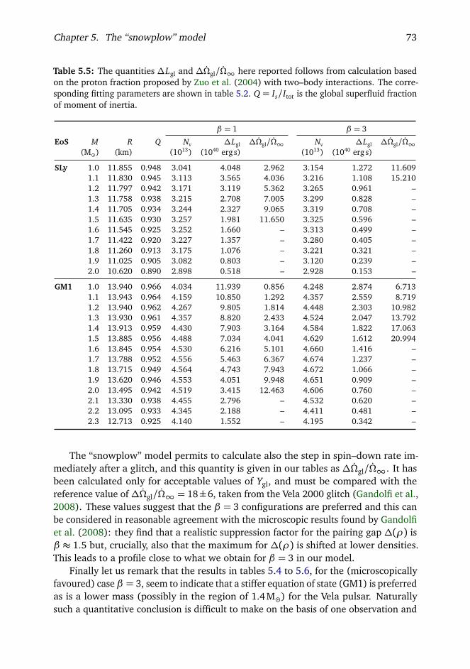
Chapter 5. The “snowplow” model 73
Table 5.5: The quantities ∆Lgl and ∆Ωgl/Ω∞ here reported follows from calculation basedon the proton fraction proposed by Zuo et al. (2004) with two–body interactions. The corre-sponding fitting parameters are shown in table 5.2. Q = Is/Itot is the global superfluid fractionof moment of inertia.
β = 1 β = 3
EoS M R Q Nv ∆Lgl ∆Ωgl/Ω∞ Nv ∆Lgl ∆Ωgl/Ω∞(M) (km) (1013) (1040 erg s) (1013) (1040 erg s)
SLy 1.0 11.855 0.948 3.041 4.048 2.962 3.154 1.272 11.6091.1 11.830 0.945 3.113 3.565 4.036 3.216 1.108 15.2101.2 11.797 0.942 3.171 3.119 5.362 3.265 0.961 –1.3 11.758 0.938 3.215 2.708 7.005 3.299 0.828 –1.4 11.705 0.934 3.244 2.327 9.065 3.319 0.708 –1.5 11.635 0.930 3.257 1.981 11.650 3.325 0.596 –1.6 11.545 0.925 3.252 1.660 – 3.313 0.499 –1.7 11.422 0.920 3.227 1.357 – 3.280 0.405 –1.8 11.260 0.913 3.175 1.076 – 3.221 0.321 –1.9 11.025 0.905 3.082 0.803 – 3.120 0.239 –2.0 10.620 0.890 2.898 0.518 – 2.928 0.153 –
GM1 1.0 13.940 0.966 4.034 11.939 0.856 4.248 2.874 6.7131.1 13.943 0.964 4.159 10.850 1.292 4.357 2.559 8.7191.2 13.940 0.962 4.267 9.805 1.814 4.448 2.303 10.9821.3 13.930 0.961 4.357 8.820 2.433 4.524 2.047 13.7921.4 13.913 0.959 4.430 7.903 3.164 4.584 1.822 17.0631.5 13.885 0.956 4.488 7.034 4.041 4.629 1.612 20.9941.6 13.845 0.954 4.530 6.216 5.101 4.660 1.416 –1.7 13.788 0.952 4.556 5.463 6.367 4.674 1.237 –1.8 13.715 0.949 4.564 4.743 7.943 4.672 1.066 –1.9 13.620 0.946 4.553 4.051 9.948 4.651 0.909 –2.0 13.495 0.942 4.519 3.415 12.463 4.606 0.760 –2.1 13.330 0.938 4.455 2.796 – 4.532 0.620 –2.2 13.095 0.933 4.345 2.188 – 4.411 0.481 –2.3 12.713 0.925 4.140 1.552 – 4.195 0.342 –
The “snowplow” model permits to calculate also the step in spin–down rate im-mediately after a glitch, and this quantity is given in our tables as ∆Ωgl/Ω∞. It hasbeen calculated only for acceptable values of Ygl, and must be compared with thereference value of∆Ωgl/Ω∞ = 18±6, taken from the Vela 2000 glitch (Gandolfi et al.,2008). These values suggest that the β = 3 configurations are preferred and this canbe considered in reasonable agreement with the microscopic results found by Gandolfiet al. (2008): they find that a realistic suppression factor for the pairing gap ∆(ρ) isβ ≈ 1.5 but, crucially, also that the maximum for ∆(ρ) is shifted at lower densities.This leads to a profile close to what we obtain for β = 3 in our model.
Finally let us remark that the results in tables 5.4 to 5.6, for the (microscopicallyfavoured) case β = 3, seem to indicate that a stiffer equation of state (GM1) is preferredas is a lower mass (possibly in the region of 1.4M) for the Vela pulsar. Naturallysuch a quantitative conclusion is difficult to make on the basis of one observation and

Chapter 5. The “snowplow” model 74
Table 5.6: The proton fraction used for this table is the three–body forces model of Zuo et al.(2004). The corresponding fitting parameters are shown in table 5.3.
β = 1 β = 3
EoS M R Q Nv ∆Lgl ∆Ωgl/Ω∞ Nv ∆Lgl ∆Ωgl/Ω∞(M) (km) (1013) (1040 erg s) (1013) (1040 erg s)
SLy 1.0 11.855 0.931 3.041 4.049 2.960 3.154 1.272 11.6071.1 11.830 0.924 3.113 3.567 4.034 3.216 1.108 –1.2 11.797 0.916 3.171 3.120 5.360 3.265 0.961 –1.3 11.758 0.908 3.215 2.708 7.002 3.299 0.828 –1.4 11.705 0.899 3.244 2.328 – 3.319 0.708 –1.5 11.635 0.888 3.257 1.981 – 3.325 0.597 –1.6 11.545 0.876 3.252 1.661 – 3.313 0.499 –1.7 11.422 0.862 3.227 1.358 – 3.280 0.405 –1.8 11.260 0.844 3.175 1.076 – 3.221 0.321 –1.9 11.025 0.820 3.082 0.803 – 3.120 0.239 –2.0 10.620 0.779 2.898 0.518 – 2.928 0.153 –
GM1 1.0 13.940 0.962 4.034 11.944 0.856 4.248 2.874 6.7121.1 13.943 0.959 4.159 10.854 1.292 4.357 2.559 8.7181.2 13.940 0.957 4.267 9.809 1.813 4.448 2.303 10.9811.3 13.930 0.953 4.357 8.824 2.432 4.524 2.047 13.7911.4 13.913 0.950 4.430 7.906 3.163 4.584 1.822 17.0611.5 13.885 0.946 4.488 7.037 4.039 4.629 1.612 –1.6 13.845 0.942 4.530 6.218 5.099 4.660 1.416 –1.7 13.788 0.937 4.556 5.465 6.365 4.674 1.237 –1.8 13.715 0.931 4.564 4.744 7.939 4.672 1.066 –1.9 13.620 0.925 4.553 4.052 9.944 4.651 0.909 –2.0 13.495 0.917 4.519 3.416 – 4.606 0.760 –2.1 13.330 0.907 4.455 2.797 – 4.532 0.620 –2.2 13.095 0.894 4.345 2.188 – 4.411 0.481 –2.3 12.713 0.873 4.140 1.553 – 4.195 0.342 –
it would be highly desirable to have information on the short-timescale post-glitchbehaviour not only of other Vela giant glitches, but also of other glitching pulsars.Note that short term components of the relaxation have not been measured for othergiant glitchers, however the “snowplow” model can be used to predict waiting times,obtaining results which are consistent with observations (Haskell et al., 2012c).
5.4 Conclusions
In this chapter we have extended the “snowplow” model for giant pulsar glitches ofPizzochero (2011) to incorporate relativistic background stellar models and realisticequations of state. In particular we have tested the model for the SLy and GM1equations of state. Unfortunately these equations of state do not include informationon beta equilibrium, so we use the proton fractions calculated by Zuo et al. (2004). Itwould of course be highly desirable to use proton fractions that are consistent with

Chapter 5. The “snowplow” model 75
the individual equations of state in future work, in order to set stringent constraints.Furthermore we have used, for the first time, the realistic profiles for the pinning forcesper unit length calculated in chapter 3, in order to evaluate the amount of angularmomentum that can be transferred to the crust during a glitch.
The model contains three free parameters, the mass of the star M , the fraction ofsuperfluid that is coupled to the crust during a glitch Ygl, and the maximum amplitudeof the pinning force, fPM. Note in fact that while the location of the maximum isprecisely determined by the microphysical calculations of chapter 3, the actual valueof the maximum can vary by factors of order unity or more as it depends on thepoorly constrained value of the vortex tension. We thus treat it as a normalization anddetermine its value by requiring that the waiting time between glitches is of 2.8 years,as is approximately the case for Vela glitches. We then fit the size of the glitch to anaverage Vela glitch to obtain the value of Ygl. In particular we take the value of theVela 2000 glitch, ∆Ω= 2.2× 10⁻⁴ rad/s (Dodson et al., 2002).
Having determined the free parameters in our model, except for the mass of theNS which is free, we compare our results to the post glitch step in frequency derivative.Unfortunately the changes in ν on short time scales after a glitch are observationallychallenging to detect and it has been possible to fit for transient steps in frequencyand frequency derivative on timescales of minutes after a glitch only for the Vela 2000and 2004 glitch (Dodson et al., 2002, 2007). Given that the detection is only barelyabove the noise for the 2004 glitch (Dodson et al., 2007) we fit to the values obtainedfor the 2000 glitch, which we assume to be a good approximation of the instantaneouspost glitch behaviour. This justifies our choice of also fitting to the value of the jumpin frequency of the Vela 2000 glitch.
The comparison of the model to the observational constraints first of all highlightsthat the general results of the analytic model of Pizzochero (2011) remain valid evenin our more physically realistic approach and the results are in general consistent forboth equations of state for a reasonable range of neutron star masses. The glitch modelpresented here thus appears robust and compatible with the observations of giantglitches in the Vela and is, as shown in Haskell et al. (2012c), compatible with theaverage waiting time between giant glitches in other pulsars. This further reinforcesthe hypothesis that giant glitches are approximately periodic phenomena that occurclose to the maximum lag that the pinning force can support in the crust, whilesmaller glitches may be triggered by random events such as crust quakes (Ruderman,1976; Ruderman et al., 1998) or vortex avalanches (Warszawski and Melatos, 2008;Melatos and Warszawski, 2009; Warszawski and Melatos, 2011, 2012a). Furthermoreour results favour lower masses for the Vela pulsar (smaller than 1.5 M) and stifferequations of state. Note however that such a quantitative conclusion is difficult to drawas not only are we comparing to a single observation but dynamical simulations havealso shown that superfluid mutual friction will contribute significantly to the shortterm post-glitch spindown as may friction at the crust/core interface (these aspectswill be discussed in chapters 8 and 9).
CHAPTER 6
Investigating superconductivitywith the snowplow model
The high density interior of a neutron star is expected to contain superconductingprotons and superfluid neutrons. Theoretical estimates suggest that the protons couldform a type II superconductor in which the stellar magnetic field is carried by flux tubes.The strong interaction between the flux tubes and the neutron rotational vortexesleads, in this case, to strong pinning, i.e. vortex motion could be impeded. This hasimportant implications especially for pulsar glitch models as it would lead to a largepart of the vorticity of the star being decoupled from the “normal” component, towhich the electromagnetic emission is locked.
In the chapter 4 we have seen that the this pinning interaction seems very low andtherefore negligible. In this regard, in the previous chapter the snowplow model hasbeen developed and applied without considering any kind of pinning force in the coreof the neutron star. Anyway, we can explore the consequences of strong pinning in thecore on the “snowplow” model, making use of same realistic equations of state andrelativistic background models (as done in the previous chapter) for the neutron star.We find that in general a large fraction of pinned vorticity in the core is not compatiblewith observations of giant glitches in the Vela pulsar. The conclusion is thus that eithermost of the core is in a type I superconducting state or that the interaction betweenvortexes and flux tubes is weaker than previously assumed (in agreement with theresults of chapter 4).
6.1 Introduction
Neutron stars allow us to probe the state of matter in some of the most extremeconditions in the universe. Not only can the density in the interior of these verycompact objects exceed nuclear saturation density, but NSs also host some of thestrongest magnetic fields in nature, with intensities of up to ≈ 1015 G for magnetars.
76
Chapter 6. Investigating superconductivity with the snowplow model 77
Not surprisingly, modelling such complex objects requires the use of some poorlyunderstood physics.
In particular the star will rapidly cool below the critical temperature for theneutrons to be superfluid and the protons to be superconducting. The protons ofthe outer core are predicted to form a type II superconductor (Migdal, 1959; Baymet al., 1969), in which the magnetic flux is confined to flux tubes, inside which themagnetic field strength is of the order of the lower critical field for superconductivity,Bc ≈ 1015 G. However, above a critical density of approximately ρc ≈ 3× 10¹⁴ g/cm3,one expects a transition to type I superconductivity, in which the formation of fluxtubesis no longer favourable but rather the magnetic field is contained in regions of normalprotons (Sedrakian, 2005). Given that the critical density for this transition is easilyreached in NS interiors it is possible that a sizeable portion of the star may in fact be ina type I superconducting state (Jones, 2006): this is the case that has been discussedin chapter 5, where the pinning phenomena was only considered in the inner crust ofthe neutron star.
An important issue to address is, however, whether vortexes will only pin to thecrustal lattice or whether they are pinned to flux tubes if the outer core is in a type IIsuperconducting state (Link, 2003), thus effectively decoupling a large fraction of thestellar moment of inertia from the crust. Furthermore if vortexes are pinned in thecore this is likely to lead to the onset of turbulence and may play an important role inpulsar ’timing noise’ (Link, 2012a). The interaction between flux tubes and vortexescan also have a strong impact on the gravitational wave driven r-mode instability (Hoet al., 2011; Haskell et al., 2012a) and on NS precession (Link, 2003).
Here we investigate the effect of vortex pinning in the core on the “snowplow”glitch model by considering a fraction of the core vorticity blocked. We implement themodel with realistic equations of state and relativistic stellar models, as in chapter 5,and show that, in general, one cannot fit the size and postglitch jumps in frequencyderivative of Vela giant glitches if a large portion of the core vortexes are pinned. Thispoints towards the fact that most of the core could in fact be in a type I superconductingstate, or that the vortex/flux tube interaction is weaker than previously assumed, asshowed in chapter 4 and as some microphysical estimates suggest (Babaev, 2009).
Furthermore Glampedakis and Andersson (2011) recently showed that vortexpinning in the core is likely to be a short lived phenomenon that may only be relevantin a short period of a NS’s life and in magnetars, and in their hydrodynamical modelof giant pulsar glitches Haskell et al. (2012c) also find that vortex pinning in the coreis inconsistent with the observed post-glitch relaxation timescales in the Vela.
6.2 The model
The starting point of our investigation will be the “snowplow” model for glitches ofPizzochero (2011), which we have explored int he previous chapter and which webriefly review here. We take the NS to be a two component system, where one of the

Chapter 6. Investigating superconductivity with the snowplow model 78
components, the so-called “normal” component, is given by the crust and all chargedcomponents tightly coupled to it by the magnetic field. The other, the “superfluid”,is given by the superfluid neutrons in the core and crust. The superfluid rotates byforming an array of quantized vortexes which carry the circulation and mediate aninteraction between the two components known as Mutual Friction, which in the corecan couple the two fluids on timescales of seconds (Andersson et al., 2006). Vortexescan, however, also be pinned to ions in the crust or flux-tubes in the core (Anderson andItoh, 1975; Alpar, 1977; Pines et al., 1980; Alpar et al., 1981; Anderson et al., 1982;Ruderman et al., 1998; Link, 2003). As a consequence vortex motion is impeded andthe superfluid cannot spin-down, effectively decoupling it from the normal componentwhich is spinning down due to electromagnetic emission. If a lag builds up betweenthe superfluid and the normal component this will, however, give rise to a Magnusforce acting on the vortexes, which takes the form fm = κρsΩ× (vv − vs), where fm isthe force per unit length, κ = 1.99× 10⁻³ cm2/s is the quantum of circulation, ρs isthe superfluid density, Ω is the unit vector pointing along the rotation axis, vv is thevelocity of the vortex lines and vs is the velocity of the superfluid. We assume thatthe neutrons are superfluid throughout the star and take ρs = (1− xp)ρ, with xp theproton fraction calculated by Zuo et al. (2004). Once the Magnus force integratedover a vortex exceeds the pinning force, the vortex will unpin and be free to move out.
We follow the procedure of chapter 5 and integrate the relativistic equations ofstellar structure for two realistic equations of state, SLy (Douchin and Haensel, 2001)and GM1 (Glendenning and Moszkowski, 1991). We assume straight vortexes thatcross through the core (Zhou et al., 2004) and for the pinning force per unit lengthfp we use the realistic estimates of chapter 3 with the profile of fig. 5.1. Balancingthe pinning force to the Magnus force and integrating over the vortex length allowsus to calculate the lag at which the vortexes will unpin in different regions. Thenormalization of fp is chosen in such a way as to give an inter-glitch waiting timeTg = ∆Ωmax/|Ω| of approximately 2.8yr for the Vela pulsar, where ∆Ωmax is themaximum of the critical unpinning lag.
If there is no pinning in the core vortexes will unpin and move out toward the crust,where they encounter a steeply increasing pinning potential and repin. This leadsto the creation of a thin vortex sheet that moves towards the peak of the potential,the so-called “snowplow” effect. Once the maximum of the critical lag has beenreached the vortexes can no longer be held in place and the excess vorticity is releasedcatastrophically, exchanging angular momentum with the normal component andgiving rise to a glitch (Pizzochero, 2011). We assume that this is the mechanism thatgives rise to giant glitches, i.e. glitches with steps in the spin rate ∆Ωgl ≈ 10−4 rad/sthat are observed in the Vela and other pulsars (Espinoza et al., 2011). Smaller glitchesare likely to be triggered by crust quakes or random vortex avalanches (Warszawskiand Melatos, 2008; Melatos and Warszawski, 2009; Warszawski and Melatos, 2011).
We can easily calculate the number of vortexes in the vortex sheet once it hasreached the peak of the potential as Nv =
2πκ r2
max∆Ωmax, where rmax is the cylindricalradius at which the maximum of the critical lag is located and ∆Ωmax the value of

Chapter 6. Investigating superconductivity with the snowplow model 79
said maximum. The angular momentum exchanged as the vortexes move out andannihilate is then given by:
∆Lgl = 2κQNv
∫ Rc
rmax
xd x
∫ l(x)/2
0
ρ(p
x2 + z2)dz (6.1)
where Q = Is/Itot is the superfluid fraction of the moment of inertia, Rc is the radiusof the inner crust where the vortexes annihilate (taken at neutron drip density), l(x)is the length of a vortex at a given cylindrical radius x and ρ is the density. The glitchobservables can then be derived as
∆Ωgl =∆L/Itot[1−Q(1− Ygl)] (6.2)
and∆Ωgl/Ω∞ = [Q(1− Ygl)]/[1−Q(1− Ygl)], (6.3)
where ∆Ωgl is the step in angular velocity due to the glitch and ∆Ωgl/Ω∞ is theinstantaneous step in the spin-down rate immediately after the glitch, relative to thesteady state pre-glitch spindown rate Ω∞. We have also introduced the parameterYgl which represents the fraction of superfluid moment of inertia which is coupledto the crust during the glitch. Given that the rise time τr is very short (less than aminute (Dodson et al., 2002)) it is likely that only a small fraction of the core willbe coupled to the crust on this short timescale, with the rest of the star recouplinggradually on longer timescales and giving rise to the observed exponential post-glitchrelaxation (see Haskell et al. (2012c) for a detailed discussion of this issue). The bestobservational upper limits on the rise time are τr < 40s (Dodson et al., 2002) fromthe Vela 2000 glitch, while an interesting lower limit of τ > 10−4 ms can be derivedfrom the non detection of a GW signal from the Vela 2006 glitch (Warszawski andMelatos, 2012a). Theoretical estimates, on the other hand, give τr ≈ 1−10 s (Haskellet al., 2012a), which thus easily allow for the angular momentum in eq. (6.1) to beexchanged during the short rise times observed in radio pulsars.
Let us now consider the motion of a vortex if the NS core is a type II superconduc-tor. As a vortex approaches a flux tube its magnetic energy will increase if they arealligned or decrease if they are antialigned reasulting in an energy per intersection ofapproximately Ep ≈ 5 MeV (Ruderman et al., 1998). Note that we have neglected thecontribution associated with the reduction of the condensation energy cost if a vortexand a flux tube overlap. This leads to an energy cost per interesection slightly smallerthan that estimated above (of the order Ep ≈ 0.1− 1 MeV) (Ruderman et al., 1998;Sidery and Alpar, 2009). Vortex motion is thus impeded by the flux tubes, that providean effective pinning barrier unless the vortexes have enough energy to cut throughthem. The corresponing pinning force per unit length of a vortex has been estimatedto be fp ≈ 3× 10¹⁵B1/2
12 dyn cm−1 (Link, 2003), and is balanced by the Magnus force
for a critical relative velocity of wc ≈ 5× 10³B1/212 cm s−1. This leads to a critical lag
(at a radius of 10 km) ∆Ωc ≈ 5× 10⁻³B1/212 rad/s, where we have assumed an average

Chapter 6. Investigating superconductivity with the snowplow model 80
density for the core of ρ = 3× 10¹⁴ g cm−3. Given the large value of the critical lag,comparable to what could be built up in-between Vela glitches, a substantial part ofthe vorticity in the core could be pinned.
To account for this effect we shall assume that a fraction of the vorticity in thecore is pinned and does not contribute to the angular momentum stored in the vortexsheet. This is equivalent to assuming that all the vorticity within a radius Rv = ηRb isfrozen, with Rb the radius of the base of the crust and η a free parameter. We thusdefine a fraction of pinned vorticity in the core as ξ= R2
v/r2max. The total number of
vortexes in the vortex sheet before the glitch scales accordingly:
Nv = (1− ξ)2πκ
r2max∆Ωmax (6.4)
By using eq. (6.4) in eq. (6.1) we can obtain the angular momentum exchanged duringthe glitch and by fitting the size of a glitch, ∆Ωgl, we can derive the coupled fractionof superfluid
Ygl =1
Q(1− ξ)
∆L∆Ωgl Itot
+Q− 1
. (6.5)
The instantaneous step in the frequency derivative then follows from
∆Ωgl
Ω∞=
Q(1− ξ)(1− Ygl)
1−Q[1− (1− ξ)Ygl](6.6)
6.3 Results
In order to compare our results with observations we consider the case of the Velapulsar. The Vela (PSR B0833-45 or PSR J0835-4510) has a spin frequency ν≈ 11.19Hzand spin-down rate ν ≈ −1.55× 10⁻¹¹ Hz s−1. Giant glitches are observed roughlyevery thousand days and have relative frequency jumps of the order ∆Ω/Ω ≈ 10−6.The spin-up is instantaneous to the accuracy of the data, with upper limits of 40 s forthe rise time obtained from the 2000 glitch (Dodson et al., 2002) and of 30 s for the2004 glitch, although this limit was less significant (Dodson et al., 2007)). The glitch isusually fitted to a model consisting of permanent steps in the frequency and frequencyderivative and a series of transient terms. It is well known that to fit the data at leastthree are required, with decay timescales that range from months to hours (Flanagan,1996). Recent observations of the 2000 and 2004 glitch have shown that an additionalterm is required on short timescales, with a decay time of approximately a minute.Given that the Vela 2000 glitch provides the most robust observational results, weshall compare the expression in eq. (6.6) to the step in frequency derivative associatedwith the short timescale (1 minute) after the Vela 2000 glitch, which we assume is areasonable approximation to the instantaneous post-glitch step in the spin down rate.The parameter Ygl is obtained from eq. (6.5) by fitting to the Vela 2000 glitch size of∆Ω/Ω= 2.2× 10⁻⁶ (Dodson et al., 2002).

Chapter 6. Investigating superconductivity with the snowplow model 81
0
2
4
6
8
10
12
14
16
18
20
22
1 1.2 1.4 1.6 1.8 2
SLY,β3
GM1,β3
SLY,β1
GM1,β1
Vela 2000
1σ
2σ
ΔΩ. gl
/ Ω. ∞
M [ MΟ• ]
(a)(b)
ξ = 0.0
0
2
4
6
8
10
12
14
16
18
20
22
1 1.2 1.4 1.6 1.8 2
SLY,β3
GM1,β3
SLY,β1
GM1,β1
Vela 2000
1σ
2σ
ΔΩ. gl
/ Ω. ∞
M [ MΟ• ]
(a)(b)
ξ = 0.2
0
2
4
6
8
10
12
14
16
18
20
22
1 1.2 1.4 1.6 1.8 2
GM1,β3
SLY,β1
GM1,β1
Vela 2000
1σ
2σ
ΔΩ. gl
/ Ω. ∞
M [ MΟ• ]
(a)(b)
ξ = 0.4
0
2
4
6
8
10
12
14
16
18
20
22
1 1.2 1.4 1.6 1.8 2
GM1,β3
SLY,β1
GM1,β1
Vela 2000
1σ
2σΔΩ. gl
/ Ω. ∞
M [ MΟ• ]
(a)(b)
ξ = 0.6
Figure 6.1: We plot the value of the fractional step in frequency derivative ∆Ω/Ω for varyingvalues of the fraction of pinned vorticity in the core, ξ for SLy and GM1. The parameter βencodes in-medium polarization effects, as described in the text. For xp we use the results ofZuo et al. (2004), both those obtained with two-body interactions (case a) and with three-bodyforces (case b). The end of the curves in these two cases corresponds to the point after which wecan no longer find a reasonable physical solution. The horizontal line represents the measuredvalue for the Vela 2000 glitch, and the thin lines are respectively 1σ and 2σ deviations. It isclear that in general both EOSs and models for the proton fraction are compatible with freevorticity in the core. As we increase the pinned fraction however it becomes increasingly moredifficult to fit the data, and for ξ > 0.5 no solution can be found at the 1σ level.
In fig. 6.1 we show the results for varying values of ξ, for both SLy and GM1. Theparameter β encodes the reduction of the pairing gap due to polarization effects inthe neutron medium. Recent calculations suggest that polarization reduces the gapand shifts the maximum to lower densities (Gandolfi et al., 2009), an effect whichin our setting corresponds to the value β ≈ 3, while β = 1 corresponds to a bareparticle approximation. The horizontal lines show the region that is allowed by themeasurements of the step in frequency derivative of the Vela 2000 glitch. It is obviousthat most equations of state and proton fractions can match this value if all vorticity inthe core is free, as was also found in the previous chapter and by Haskell et al. (2012c),although we note that for the more realistic case of β = 3 and three body casesincluded in the calculation of xp, the stiffer equation of state is clearly favored. Wenow compare this to the case in which part of the core is in a type II superconductingstate and part of the vorticity is pinned. As we can see from fig. 6.1, as the parameter

Chapter 6. Investigating superconductivity with the snowplow model 82
ξ increases it becomes increasingly harder to fit the observed values of ∆Ω and inmost cases this is only possible for a very restricted interval of masses. In generalone cannot obtain a physically reasonable fit if more than half of the vorticity in thecore is pinned. This points to the conclusion that the vortex/flux tube interaction isweaker than previously assumed and that most of the vorticity in the core is, in fact,free. This conclusion is compatible with that of Haskell et al. (2012c), who found thata weak coupling between the superfluid and normal component in the core (as wouldbe the case if most of the vortexes in the core are pinned) does not allow to fit theshorter post-glitch relaxation timescales of the Vela. Note that the conclusions of thisLetter and those of Haskell et al. (2012c) are derived in different methods (in thiscase calculating the exchange of angular momentum in a static model, in the case ofHaskell et al. (2012c) by fitting the post-glitch relaxation with a dynamical multifluidmodel) and are thus independent, save for the use of the pinning forces calculated inGrill (2011); Grill and Pizzochero (2012).
6.4 Conclusions
In this chapter we have extended the “snowplow” model Pizzochero (2011) discussedin the previous chapter, to account for the possibility that part of the vorticity in thecore may be pinned due to the interaction between vortexes and flux tubes. We fitthe step in frequency and in frequency derivative of the Vela 2000 glitch to obtainconstraints on the pinned fraction of vortexes in the core and in general find that bothquantities cannot be fitted for reasonable physical parameters if the pinned fraction islarger than 50%. Although we do not deal with the microphysical details of the vortexdynamics in the core, our conclusions are quite general. The only quantity that isneeded to evaluate the angular momentum that is exchanged during a glitch is, in fact,the number of vortexes that are stored close to the peak of the pinning potential in thecrust. As long as the excess vorticity of the core can be transferred to the equatorialstrong pinning region in-between glitches the details of the vortex motion are notinfluential.
The general conclusion is that either most of the core is in a type I superconductingstate (and the vortex pinning is negligible (Sedrakian, 2005)), or that the vortex/fluxtube interaction is weaker than previously thought. This is the same conclusion thatHaskell et al. (2012c) come to after fitting the post-glitch short-term relaxation of Velaglitches with a hydrodynamical model. If such an conclusion is confirmed it wouldhave serious implications also for NS precession (Link, 2003) and for GW emission(Haskell et al., 2008; Lander et al., 2012; Ho et al., 2011; Haskell et al., 2012a). Notethat on a microphysical level it is very likely that the interaction between vortexes andflux tubes is weaker than the previous estimates presented here. These estimates areupper limits on the strength of the pinning force, as they do not account for the finiterigidity of vortexes, which could lead to a reduction of a factor 100-1000, as theoreticalestimates in chapter 4 also confirm. Furthermore recent calculations (Babaev, 2009)
Chapter 6. Investigating superconductivity with the snowplow model 83
suggest that in the presence of strong entrainment or gapped Σ− hyperons in thecrust the interaction between flux tubes and vortexes will be significantly weaker, andeven in the presence of pinning the superfluid may be coupled to the crust on shorttimescales (Sidery and Alpar, 2009).
CHAPTER 7Measuring neutron star masses
with pulsar glitches
In this chapter we want to extend the snowplow model described previously in orderto overcome its limitations. The paradigm proposed till now use the two componentapproach together with a realistic macroscopic scenario (spherical geometry, densityprofile from TOV equilibrium with realistic EOSs, density-dependent pinning andMagnus forces) and with the assumption (microscopically better justified) of contin-uous vortexes across the core and the crust. The strength of this perspective is itssimplicity, with at the same time the ability of identify a storing mechanism for theangular momentum of neutron vortexes that it suddenly released to the crust at theglitch. The angular momentum reservoir is created by the existence of clear peak inthe critical lag profile, obtained by equating the pinning force acting on a vortex withthe Magnus force that tends to push it outward. The plots of fig. 5.5 clearly show thispeak: the strong pinning barrier in the crust and the flat profile in the core (conse-quence of the assumption of continuous vortexes) suggest the snowplow mechanism.In the time between two glitches the actual lags builds up and the depinning regionbecomes larger, pushing a thin vortex sheet (that actually store the angular momentumexchanged during the glitch) toward the maximum of the critical lag. When thismaximum is reached we have a glitch because there is no more strong pinning regionthat can stop the vortexes from reaching the crust: the vortexes in the thin sheet unpinsimultaneously and a vortex avalanche starts down the peak. The glitch event relaxesthe two components of the star, reducing the lag and allowing the vorticity in the coreto be repinned: this is important because in this way the process can repeat itself.
Following this approach it’s possible to calculate the number of vortexes storedand their angular momentum (see eq. (5.11)) and consequently the jump size ∆Ωgl ofthe glitch. The model relay on two free parameters: the maximum value pinning forcefPM and the fraction of vorticity coupled to the normal crust during the glitch, Ygl. Inchapter 5 we proceeded by fixing the value of fPM in order to reproduce the averagewaiting time between glitches observed for the Vela pulsar, while the recorded jump
84

Chapter 7. Measuring neutron star masses with pulsar glitches 85
in Ω was used to infer the value of Ygl (referred to the Vela 2000 glitch, see (Dodsonet al., 2002)).
The snowplow model is a consistent mechanism for vortex accumulation andthence a realistic description of the angular momentum reservoir, which is needed toexplain the glitch phenomenon. However, it is not a plausible description of the actualtrigger mechanism, since it predicts a constant period between glitches and thereforeit cannot reproduce the wide distribution of intervals between glitches observed inreality. Moreover, the statistical studies of Melatos and Warszawski (2009) indicate thatthe distribution of glitch sizes and times are compatible with the behavior of criticalsystems and that several glitch triggers appear as possible (vortex knock–on, acousticwaves, etc). Therefore, in this revised version of the snowplow model proposed here,we leave the trigger as a unknown mechanism, whose origin and timing propertiesare still to be determined. We use the snowplow scenario of vortex accumulation inan outward moving sheet to evaluate the angular momentum stored in the crust as afunction of the time passed from the previous glitch. This yields the maximum value ofa glitch if all the excess vorticity removed from the core and accumulated at the sheetwas released at that time and its angular momentum was transferred instantaneouslyto the crust.
The main feature of the snowplow model that remains valid here is the vortexsheet, namely a thin cylindrical shell of more–than–average vortex density, dynamicallyout of equilibrium and moving outwards against the pinning potential, driven by theincreasing lag associated to the crust secular spin-down. On one hand, it provides forthe first time a realistic mechanism to store the angular momentum which is necessaryto justify the occurrence of a glitch. On the other hand, the presence of the vortexsheet may be crucial in the trigger mechanism; indeed, triggering the catastrophic andsimultaneous unpinning of the accumulated excess vorticity appears simpler whenthis is concentrated in a thin cylindrical shell, rather than being diffused all across thecrust.
7.1 The entrainment in the snowplow paradigm
In chapter 5 we used a simple profile for the pinning force per unit length that wasscaled in order to obtain the corrected waiting time. Here we leave the trigger asan unknown mechanism that cause a glitch at a arbitrary time t after the previousone: there is no prescription to perform a fitting on the pinning force and thereforewe will use here the realistic profiles obtained in chapter 3 for the configurationL = 5000,β = 3, that is microscopically favoured (see also considerations in chapter 5and (Gandolfi et al., 2008)). The values used are reported in fig. 3.11 and in table 3.3.
An important aspect that was neglected in the original model is superfluid en-trainment. As showed by Andersson et al. (2012) the presence of this non–dissipativecoupling between the neutron fluid and the proton one can’t be neglected and it isimportant to explain observational data. The effect of entrainment can be represented

Chapter 7. Measuring neutron star masses with pulsar glitches 86
0
2
4
6
8
10
12
14
0 1.0⋅10-2 2.0⋅10-2 3.0⋅10-2 4.0⋅10-2 5.0⋅10-2 6.0⋅10-2 7.0⋅10-2 8.0⋅10-2
mn* /
mn
nb [fm-3]
mn*/mn
Figure 7.1: Plot of the entrainment effective neutron mass m∗n/mn as a function of the bariondensity nb (Chamel, 2006). These values will be used here and in the following to model theentrainment effect in a neutron star crust.
by a neutron effective mass, m∗n(ρ), and we introduce it in the snowplow model in thestandard way, by reducing locally the neutron-proton velocity lag for pinned vorticity.We will use for m∗n(ρ) the recent values calculated by Chamel (2012) for the crust ofneutron stars. The values of m∗n are given by the author as a function of the bariondensity nb (see fig. 7.1 for a plot of the ratio m∗n/mn versus nb). The barion densitycan be related to the density ρ following the considerations suggested by Haenseland Potekhin (2004) for a thermodynamically consistent EOS that lead to the thisequation:
nb(r) =1
mn
ρ(r) +P(r)c2
eΦ(r)−Φ(R) (7.1)
where Φ(r) =p
1− 2GM/(Rc2). As done in previous chapters, we obtain a realisticstar by integrating the TOV equations with SLy and GM1 as equations of state, thanthe eq. (7.1) lets us assign a value to the effective neutron mass m∗n for every radius r.
The range of density covered by Chamel (2012) is the typical one of the inner crustof a neutron star. Recent calculations by the same author (Chamel, 2006) suggest thatthe proton effective mass is slightly lower than the bare mass in the core but can belarger in the crust. This means that the entrainment parameters will vanish close tothe base of the crust (Carter et al., 2006): we can therefore consider the m∗n = mn inthe core of the star.

Chapter 7. Measuring neutron star masses with pulsar glitches 87
In a simple global two fluid model, the entrainment affects the dynamics with anondissipative coupling between the fluids that can be modeled with the followingequations (see also Andersson et al. (2012)):
(Ip − εn In)Ωp + εn InΩn = −aΩ3p −Ψ(r) (7.2)
(In − εn In)Ωn + εn InΩp = Ψ(r) (7.3)
where Ψ encodes pinning, drag forces and eventually other dissipative interactions.It’s clear from these equations that a fraction of the neutron component behaves as theproton one; the coefficient of this coupling is εn that is strictly related to the effectiveneutron mass:
εn = 1−Ým∗n (7.4)
where Ým∗n =m∗nmn
. In case of perfect pinning, the left side of eq. (7.3) vanishes (it’s easyto verify that in case εp = 0 the standard condition used in the snowplow model isreproduced, see chapter 5). This means that even if the vortexes are pinned to thecrust, the macroscopic angular velocity of the neutron fluid decrease as a consequenceof the coupling with the protons. This is the main effect of the entrainment:
Ωn = −εn
1− εnΩp (7.5)
From this equation it’s possible to calculate the actual lag developed in the star interiorsfor a time t after a glitch: we call ω the raw lag expressed as ω = |Ωp|t and correct itto take into account the entrainment:
∆Ω(t) = (Ωn − Ωp)t =
−εn
1− εn− 1
Ωp t =ω
Ým∗n(7.6)
As described before, we consider an unspecified trigger for the glitch that happensat a time t after the previous one. At this time, the lag ∆Ω(t) built by the star hasdepinned the inner region of the star, before the vortex sheet that is placed at theposition x∗(t), as explained by the fig. 7.2. In order to estimate the glitch size, weconsider that the angular momentum transferred to the crust is that of the shadedregion in the plot: this represent the excess of vorticity after the vortex sheet that iscompletely removed by the catastrophic avalanche. From eq. (2.21) eq. (2.22) we canexpress this quantity in the following way:
∆Lgl(t) =
∫
min(ω(t)/Ým∗n,∆Ωcr) x2ρn(x , z) dV (7.7)
where the integration must be done in the cylindrical region outside the vortex sheetposition x∗. With the usual cylindrical coordinates this becomes
∆Lgl(t) = 2π
∫ Ric
x∗x3 d x
∫ `(x)
0
min(|Ωp|t,Ým∗n(x , z)∆Ωcr(x))ρn(x , z)Ým∗n(x , z)
dz. (7.8)

Chapter 7. Measuring neutron star masses with pulsar glitches 88
1.0⋅10-5
1.0⋅10-4
1.0⋅10-3
1.0⋅10-2
1.0⋅10-1
8 8.5 9 9.5 10 10.5 11 11.5 12
x*
t -> lag = |Ω.p|t/m*
ΔΩ
[ra
d/s]
x [105 cm]
ΔΩcr (x)ΔΩ
Figure 7.2: This plot shows the critical lag profile of a 1.4M GM1 star, as a function of thecylindrical radius x . The shaded region indicates the vorticity involved in the calculation of theangular momentum ∆Lgl(t) transferred to the crust at the glitch (t represent the interglitchtime).
Now it’s easy to calculate the jump in angular velocity at the glitch, as in chapter 5:∆Ωgl(t) =∆Lgl(t)/Ieff, where again the effective momentum of inertia used is
Ieff = (1−Q)Itot +QYgl Itot. (7.9)
This approach leaves us with only one free parameter: after choosing the EOS and themass of the neutron star, the remaining free quantity is the coupled vorticity Ygl.
The result of this revised snowplow model is a function ∆Ωgl(t) representing themaximum possible glitch size as a function of the time passed since the previousglitch. All actual glitches must lie below this curve, since vortex avalanches arerarely maximal, as discussed by Espinoza et al. (2011). The vorticity accumulated atthe sheet is released simultaneously by the trigger and initiates a global avalanchewhile the vortex sheet is disrupted, but the avalanche itself may develop in differentways. The snowplow model only provides an upper bound for the glitch size, whilethe triggering and the dynamics of vortex avalanches are probably better studied bystatistical methods suitable for critical systems.
In the fig. 7.3 is plotted the curves ∆Ωgl(t) for different choices of the free param-eter Ygl. We choose to plot the quantity against the raw lag ω = |Ωp|t, instead thesimple interval t between glitches, in order to easily compare the results obtained fora star with the ones obtained for a neutron star with different slowdown. As explained

Chapter 7. Measuring neutron star masses with pulsar glitches 89
0
1⋅10-4
2⋅10-4
3⋅10-4
4⋅10-4
5⋅10-4
6⋅10-4
7⋅10-4
8⋅10-4
0 2⋅10-3 4⋅10-3 6⋅10-3 8⋅10-3 1⋅10-2 1⋅10-2 1⋅10-2 2⋅10-2 2⋅10-2 2⋅10-2
(1)(2)(3)(4)
ΔΩ
gl [
rad/
s]
ω [rad/s]
(1) Ygl = 0.08(2) Ygl = 0.10(3) Ygl = 0.12(4) Ygl = 0.14
B0833-45B0833-45 mean
Figure 7.3: Plot of the curves ∆Ωgl(t) obtained with different values of the parameter Ygl.All these results are referred to the same 1.3M GM1 star. The dots represent the observedglitches of the Vela pulsar.
before, this is not the actual lag developed, due to the presence of the entrainment. Inthis plot we report, together with the calculated curves, also the observational data ofthe Vela Pulsar B0833–45: every point represents a recorded glitch, with its jump sizein ordinate and the interglitch time multiplied by |Ωp| on the x axis (for this pulsar theaverage slowdown is Ωp = −9.84324× 10⁻¹¹ rad/s2, see Manchester et al. (2005)).To obtain these curves, we have fixed the mass of the star to be M = 1.3 M. Ananalogous approach has been used to test the effect of the parameter M : in fig. 7.4 wechange the value of the mass of the star, keeping fixed the fraction of coupled vorticityYgl = 0.10.
From the plots it’s clear that both parameters control the value of the jump sizefor a given waiting time. Increasing the fraction of coupled vorticity lowers the curvein the plot discussed previously, i.e. reduce ∆Ωgl consistently for every time t. Theeffect of the mass is pretty much the same: a massive star will show smaller glitchesfor every waiting time considered, due to the fact that the shape of the curve remainsnearly the same.

Chapter 7. Measuring neutron star masses with pulsar glitches 90
0
2⋅10-4
4⋅10-4
6⋅10-4
8⋅10-4
1⋅10-3
1⋅10-3
0 2⋅10-3 4⋅10-3 6⋅10-3 8⋅10-3 1⋅10-2 1⋅10-2 1⋅10-2 2⋅10-2 2⋅10-2 2⋅10-2
(1)
(2)(3)(4)
ΔΩ
gl [
rad/
s]
ω [rad/s]
(1) M = 1.10(2) M = 1.30(3) M = 1.50(4) M = 1.70
B0833-45B0833-45 mean
Figure 7.4: Plot of the curves ∆Ωgl(t) obtained with different values of the total mass M ofthe star. All these results are calculated keeping fixed Ygl = 0.10 and all other parameters. Thedots represent the observed glitches of the Vela pulsar.
7.2 Fitting of NS masses with the snowplow model
The considerations exposed in the previous section can be used now to infer themass of a neutron star in the following way. For this purpose we consider the 15youngest neutron stars among the set of the frequent glitchers (we define with thisterm the pulsars with at least 5 observed glitches) detailed in table 7.2. These pulsarsare the first 15 rows of the table (the column τ reports the age of the pulsar). Asexplained before, we use a fixed pinning profile obtained from the realistic mesoscopiccalculations done in chapter 3 (L = 5000 Rws, β = 3), and therefore, once we havefixed the equation of state, we have only two free parameters, namely the mass Mand the fraction of coupled vorticity Ygl. For the EoS we will adopt, as usually, thestiff GM1 or the softer SLy. From the results in chapter 2 we can see that the first oneadmits a larger maximum mass Mmax = 2.36 M, while for the other Mmax = 2.05M.
For each of the 15 younger glitchers, we can plot the observed ∆Ωi vs ωi = |Ω|τi ,where τi is the time elapsed from the previous glitch, as well as the curve ∆Ωgl(ω).As explained, the observed glitches cannot lie above the theoretical upper limit repre-sented by the curve; then we proceed as follows to remove the degeneracy related tothe two free parameters:
1. we set the mass of Vela at some value MVela; then we vary Ygl until the calculated

Chapter 7. Measuring neutron star masses with pulsar glitches 91
curve ∆Ωgl(ω) is tangent to the largest observed glitch in Vela.
2. we fix Ygl at the value found for Vela; then, for each of the other 14 objects, wevary the mass M until the curve is tangent to the largest observed glitch in eachobject.
The procedure is shown in fig. 7.5 and fig. 7.6 where we have used SLy as EOS;and in fig. 7.7 and fig. 7.8 for the stiffer equation of state GM1. In both cases wehave set the mass of Vela to be MVela = 1.3M, and the mass fitting was made with adiscrete step of 0.01 M. In the figures we also plot the position of the vortex sheet,X (t) (scale on the right ordinate axis), as a function of the lag; two gray horizontallines indicate the inner and outer radius of the inner crust. Repeating this for all the15 glitchers and testing both EOSs, we find that:
• most glitchers can be fitted with a mass smaller than Mmax. The only exceptionsare B1758 and B1737, for which all the observed glitches are well below thecurve ∆Ωgl(ω) corresponding to Mmax;
• in the stronger glitchers, the events are triggered when the vortex sheet iscompletely immersed in the crust (curve X (t) between the two horizontal lines);in the weaker objects, the glitches are triggered when the vortex sheet is mostlyimmersed in the core, with only the vortex extremities pinned in the crust.Due to the strong entrainment and the realistic values for the pinning force wecan conclude that these glitches are always triggered well before reaching themaximum of the pinning potential.
The inferred values of the masses of the considered pulsars are summarized intable 7.1. Since we are fitting the maximal glitches, which are absolute lower limits,the masses we obtain are absolute upper limits: any future larger glitch can onlyreduce the value obtained here. We have chosen initially to set the mass for Vela atMVela = 1.3M. Nevertheless, we have also tested the model by fixing MVela = 1.2M:we have observed that this produce a coherent shift by 0.1 M on all the other calculatedmasses, and therefore the considerations exposed in the next section remain valid:here we will discuss these results in connection with the other observable quantitiesof the pulsars (see table 7.2). The results presented here are obtained with Ygl = 0.02for SLy and Ygl = 0.10 for the GM1 equation of state, values that are reasonable andin perfect agreement with the results of chapter 5.
We want to highlight here the role of the entrainment in the model. In fig. 7.9 wesee the curve∆Ωgl(t) in two cases: with the entrainment and without the entrainment.The result is immediately clear: in the configuration without the entrainment there isno chance of fitting all the observational data, because the curve in the plot is “tooshort”. Changing the free parameters of the model, M and Ygl would not help much,because they only shift vertically the curve. The value of ωend where the curve stopsis of course strictly related to the value of the peak of the critical unpinning lag of thestar: when the built lag reaches the peak of the critical lag, the star must exhibit its
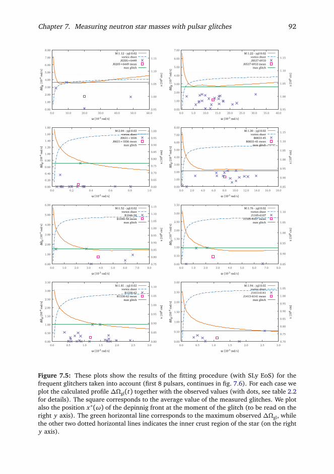
Chapter 7. Measuring neutron star masses with pulsar glitches 92
0.00
1.00
2.00
3.00
4.00
5.00
6.00
7.00
8.00
0.0 10.0 20.0 30.0 40.0 50.0 60.00.95
1.00
1.05
1.10
1.15
ΔΩ
gl [
10-4
rad
/s]
x [1
06 cm
]
ω [10-3 rad/s]
M:1.12 - ygl:0.02vortex sheet
J0205+6449J0205+6449 mean
max glitch
0.00
1.00
2.00
3.00
4.00
5.00
6.00
7.00
0.0 5.0 10.0 15.0 20.0 25.0 30.0 35.0 40.00.95
1.00
1.05
1.10
1.15
ΔΩ
gl [
10-4
rad
/s]
x [1
06 cm
]
ω [10-3 rad/s]
M:1.22 - ygl:0.02vortex sheetJ0537-6910
J0537-6910 meanmax glitch
0.00
0.20
0.40
0.60
0.80
1.00
1.20
1.40
1.60
1.80
0.0 0.2 0.4 0.6 0.8 1.00.60
0.65
0.70
0.75
0.80
0.85
0.90
0.95
1.00
ΔΩ
gl [
10-4
rad
/s]
x [1
06 cm
]
ω [10-3 rad/s]
M:2.04 - ygl:0.02vortex sheet
J0631+1036J0631+1036 mean
max glitch
0.00
1.00
2.00
3.00
4.00
5.00
6.00
7.00
8.00
0.0 2.0 4.0 6.0 8.0 10.0 12.0 14.0 16.0 18.00.85
0.90
0.95
1.00
1.05
1.10
1.15
ΔΩ
gl [
10-4
rad
/s]
x [1
06 cm
]
ω [10-3 rad/s]
M:1.30 - ygl:0.02vortex sheet
B0833-45B0833-45 mean
max glitch
0.00
1.00
2.00
3.00
4.00
5.00
6.00
0.0 1.0 2.0 3.0 4.0 5.0 6.0 7.0 8.00.75
0.80
0.85
0.90
0.95
1.00
1.05
1.10
1.15
ΔΩ
gl [
10-4
rad
/s]
x [1
06 cm
]
ω [10-3 rad/s]
M:1.52 - ygl:0.02vortex sheet
B1046-58B1046-58 mean
max glitch
0.00
0.50
1.00
1.50
2.00
2.50
3.00
3.50
0.0 1.0 2.0 3.0 4.0 5.0 6.0 7.0 8.00.85
0.90
0.95
1.00
1.05
1.10
ΔΩ
gl [
10-4
rad
/s]
x [1
06 cm
]
ω [10-3 rad/s]
M:1.76 - ygl:0.02vortex sheetJ1105-6107
J1105-6107 meanmax glitch
0.00
0.50
1.00
1.50
2.00
2.50
3.00
3.50
0.0 0.5 1.0 1.5 2.0 2.5 3.00.80
0.85
0.90
0.95
1.00
1.05
1.10
ΔΩ
gl [
10-4
rad
/s]
x [1
06 cm
]
ω [10-3 rad/s]
M:1.81 - ygl:0.02vortex sheet
B1338-62B1338-62 mean
max glitch
0.00
0.50
1.00
1.50
2.00
2.50
3.00
0.0 0.5 1.0 1.5 2.0 2.5 3.00.70
0.75
0.80
0.85
0.90
0.95
1.00
1.05
ΔΩ
gl [
10-4
rad
/s]
x [1
06 cm
]
ω [10-3 rad/s]
M:1.94 - ygl:0.02vortex sheetJ1413-6141
J1413-6141 meanmax glitch
Figure 7.5: These plots show the results of the fitting procedure (with SLy EoS) for thefrequent glitchers taken into account (first 8 pulsars, continues in fig. 7.6). For each case weplot the calculated profile ∆Ωgl(t) together with the observed values (with dots, see table 2.2for details). The square corresponds to the average value of the measured glitches. We plotalso the position x∗(ω) of the depinnig front at the moment of the glitch (to be read on theright y axis). The green horizontal line corresponds to the maximum observed ∆Ωgl, whilethe other two dotted horizontal lines indicates the inner crust region of the star (on the righty axis).

Chapter 7. Measuring neutron star masses with pulsar glitches 93
0.00
1.00
2.00
3.00
4.00
5.00
6.00
7.00
0.0 2.0 4.0 6.0 8.0 10.0 12.0 14.00.85
0.90
0.95
1.00
1.05
1.10
1.15
ΔΩ
gl [
10-4
rad
/s]
x [1
06 cm
]
ω [10-3 rad/s]
M:1.39 - ygl:0.02vortex sheetJ1420-6048
J1420-6048 meanmax glitch
0.00
0.20
0.40
0.60
0.80
1.00
1.20
1.40
1.60
1.80
2.00
0.0 0.1 0.2 0.3 0.4 0.5 0.6 0.7 0.8 0.90.55
0.60
0.65
0.70
0.75
0.80
0.85
0.90
0.95
1.00
ΔΩ
gl [
10-4
rad
/s]
x [1
06 cm
]
ω [10-3 rad/s]
M:2.04 - ygl:0.02vortex sheet
B1737-30B1737-30 mean
max glitch
0.00
1.00
2.00
3.00
4.00
5.00
6.00
7.00
8.00
9.00
0.0 1.0 2.0 3.0 4.0 5.0 6.0 7.0 8.0 9.00.65
0.70
0.75
0.80
0.85
0.90
0.95
1.00
1.05
1.10
1.15
ΔΩ
gl [
10-4
rad
/s]
x [1
06 cm
]
ω [10-3 rad/s]
M:1.37 - ygl:0.02vortex sheet
B1757-24B1757-24 mean
max glitch
0.00
0.20
0.40
0.60
0.80
1.00
1.20
1.40
1.60
1.80
2.00
0.0 0.1 0.2 0.3 0.4 0.5 0.6 0.7 0.8 0.90.55
0.60
0.65
0.70
0.75
0.80
0.85
0.90
0.95
1.00
ΔΩ
gl [
10-4
rad
/s]
x [1
06 cm
]
ω [10-3 rad/s]
M:2.04 - ygl:0.02vortex sheet
B1758-23B1758-23 mean
max glitch
0.00
1.00
2.00
3.00
4.00
5.00
6.00
7.00
8.00
0.0 2.0 4.0 6.0 8.0 10.0 12.0 14.00.80
0.85
0.90
0.95
1.00
1.05
1.10
1.15
ΔΩ
gl [
10-4
rad
/s]
x [1
06 cm
]
ω [10-3 rad/s]
M:1.32 - ygl:0.02vortex sheet
B1800-21B1800-21 mean
max glitch
0.00
1.00
2.00
3.00
4.00
5.00
6.00
0.0 5.0 10.0 15.0 20.00.90
0.95
1.00
1.05
1.10
1.15
ΔΩ
gl [
10-4
rad
/s]
x [1
06 cm
]
ω [10-3 rad/s]
M:1.39 - ygl:0.02vortex sheet
B1823-13B1823-13 mean
max glitch
0.00
0.50
1.00
1.50
2.00
2.50
3.00
3.50
4.00
4.50
0.0 5.0 10.0 15.0 20.00.90
0.95
1.00
1.05
1.10
1.15
ΔΩ
gl [
10-4
rad
/s]
x [1
06 cm
]
ω [10-3 rad/s]
M:1.49 - ygl:0.02vortex sheet
J2229+6114J2229+6114 mean
max glitch
Figure 7.6: These plots complete the results of fig. 7.5 and therefore they are referred to theSLy equation of state. See fig. 7.5 for details.

Chapter 7. Measuring neutron star masses with pulsar glitches 94
0.00
1.00
2.00
3.00
4.00
5.00
6.00
7.00
8.00
9.00
10.00
0.0 10.0 20.0 30.0 40.0 50.0 60.01.00
1.05
1.10
1.15
1.20
1.25
1.30
1.35
ΔΩ
gl [
10-4
rad
/s]
x [1
06 cm
]
ω [10-3 rad/s]
M:1.05 - ygl:0.10vortex sheet
J0205+6449J0205+6449 mean
max glitch
0.00
1.00
2.00
3.00
4.00
5.00
6.00
7.00
8.00
0.0 5.0 10.0 15.0 20.0 25.0 30.0 35.0 40.00.95
1.00
1.05
1.10
1.15
1.20
1.25
1.30
1.35
ΔΩ
gl [
10-4
rad
/s]
x [1
06 cm
]
ω [10-3 rad/s]
M:1.20 - ygl:0.10vortex sheetJ0537-6910
J0537-6910 meanmax glitch
0.00
0.20
0.40
0.60
0.80
1.00
1.20
1.40
1.60
0.0 0.2 0.4 0.6 0.8 1.00.70
0.80
0.90
1.00
1.10
1.20
ΔΩ
gl [
10-4
rad
/s]
x [1
06 cm
]
ω [10-3 rad/s]
M:2.33 - ygl:0.10vortex sheet
J0631+1036J0631+1036 mean
max glitch
0.00
1.00
2.00
3.00
4.00
5.00
6.00
7.00
8.00
9.00
10.00
0.0 2.0 4.0 6.0 8.0 10.0 12.0 14.0 16.0 18.00.60
0.70
0.80
0.90
1.00
1.10
1.20
1.30
ΔΩ
gl [
10-4
rad
/s]
x [1
06 cm
]
ω [10-3 rad/s]
M:1.30 - ygl:0.10vortex sheet
B0833-45B0833-45 mean
max glitch
0.00
0.50
1.00
1.50
2.00
2.50
3.00
3.50
4.00
4.50
0.0 1.0 2.0 3.0 4.0 5.0 6.0 7.0 8.00.95
1.00
1.05
1.10
1.15
1.20
1.25
1.30
1.35
ΔΩ
gl [
10-4
rad
/s]
x [1
06 cm
]
ω [10-3 rad/s]
M:1.61 - ygl:0.10vortex sheet
B1046-58B1046-58 mean
max glitch
0.00
0.50
1.00
1.50
2.00
2.50
3.00
3.50
0.0 1.0 2.0 3.0 4.0 5.0 6.0 7.0 8.00.85
0.90
0.95
1.00
1.05
1.10
1.15
1.20
1.25
1.30
1.35
ΔΩ
gl [
10-4
rad
/s]
x [1
06 cm
]
ω [10-3 rad/s]
M:1.91 - ygl:0.10vortex sheetJ1105-6107
J1105-6107 meanmax glitch
0.00
0.50
1.00
1.50
2.00
2.50
3.00
0.0 0.5 1.0 1.5 2.0 2.5 3.00.90
0.95
1.00
1.05
1.10
1.15
1.20
1.25
1.30
1.35
ΔΩ
gl [
10-4
rad
/s]
x [1
06 cm
]
ω [10-3 rad/s]
M:1.96 - ygl:0.10vortex sheet
B1338-62B1338-62 mean
max glitch
0.00
0.50
1.00
1.50
2.00
2.50
0.0 0.5 1.0 1.5 2.0 2.5 3.00.85
0.90
0.95
1.00
1.05
1.10
1.15
1.20
1.25
1.30
ΔΩ
gl [
10-4
rad
/s]
x [1
06 cm
]
ω [10-3 rad/s]
M:2.10 - ygl:0.10vortex sheetJ1413-6141
J1413-6141 meanmax glitch
Figure 7.7: These plots show the results of the fitting procedure (with GM1 EoS) for thefrequent glitchers taken into account (first 8 pulsars, continues in fig. 7.8). For each case weplot the calculated profile ∆Ωgl(t) together with the observed values (with dots, see table 2.2for details). The square corresponds to the average value of the measured glitches. We plotalso the position x∗(ω) of the depinnig front at the moment of the glitch (to be read on theright y axis). The green horizontal line corresponds to the maximum observed ∆Ωgl, whilethe other two dotted horizontal lines indicates the inner crust region of the star (on the righty axis).

Chapter 7. Measuring neutron star masses with pulsar glitches 95
0.00
1.00
2.00
3.00
4.00
5.00
6.00
0.0 2.0 4.0 6.0 8.0 10.0 12.0 14.01.00
1.05
1.10
1.15
1.20
1.25
1.30
1.35
ΔΩ
gl [
10-4
rad
/s]
x [1
06 cm
]
ω [10-3 rad/s]
M:1.38 - ygl:0.10vortex sheetJ1420-6048
J1420-6048 meanmax glitch
0.00
0.20
0.40
0.60
0.80
1.00
1.20
0.0 0.1 0.2 0.3 0.4 0.5 0.6 0.7 0.8 0.90.70
0.75
0.80
0.85
0.90
0.95
1.00
1.05
1.10
1.15
1.20
ΔΩ
gl [
10-4
rad
/s]
x [1
06 cm
]
ω [10-3 rad/s]
M:2.36 - ygl:0.10vortex sheet
B1737-30B1737-30 mean
max glitch
0.00
1.00
2.00
3.00
4.00
5.00
6.00
7.00
0.0 1.0 2.0 3.0 4.0 5.0 6.0 7.0 8.0 9.00.80
0.90
1.00
1.10
1.20
1.30
ΔΩ
gl [
10-4
rad
/s]
x [1
06 cm
]
ω [10-3 rad/s]
M:1.42 - ygl:0.10vortex sheet
B1757-24B1757-24 mean
max glitch
0.00
0.20
0.40
0.60
0.80
1.00
1.20
0.0 0.1 0.2 0.3 0.4 0.5 0.6 0.7 0.8 0.90.70
0.75
0.80
0.85
0.90
0.95
1.00
1.05
1.10
1.15
1.20
ΔΩ
gl [
10-4
rad
/s]
x [1
06 cm
]
ω [10-3 rad/s]
M:2.36 - ygl:0.10vortex sheet
B1758-23B1758-23 mean
max glitch
0.00
1.00
2.00
3.00
4.00
5.00
6.00
7.00
8.00
0.0 2.0 4.0 6.0 8.0 10.0 12.0 14.00.90
0.95
1.00
1.05
1.10
1.15
1.20
1.25
1.30
1.35
ΔΩ
gl [
10-4
rad
/s]
x [1
06 cm
]
ω [10-3 rad/s]
M:1.29 - ygl:0.10vortex sheet
B1800-21B1800-21 mean
max glitch
0.00
1.00
2.00
3.00
4.00
5.00
6.00
7.00
0.0 5.0 10.0 15.0 20.00.90
0.95
1.00
1.05
1.10
1.15
1.20
1.25
1.30
1.35
ΔΩ
gl [
10-4
rad
/s]
x [1
06 cm
]
ω [10-3 rad/s]
M:1.39 - ygl:0.10vortex sheet
B1823-13B1823-13 mean
max glitch
0.00
1.00
2.00
3.00
4.00
5.00
6.00
0.0 5.0 10.0 15.0 20.00.95
1.00
1.05
1.10
1.15
1.20
1.25
1.30
1.35
ΔΩ
gl [
10-4
rad
/s]
x [1
06 cm
]
ω [10-3 rad/s]
M:1.51 - ygl:0.10vortex sheet
J2229+6114J2229+6114 mean
max glitch
Figure 7.8: These plots complete the results of fig. 7.7 and therefore they are referred to theGM1 equation of state. See fig. 7.7 for details.

Chapter 7. Measuring neutron star masses with pulsar glitches 96
Table 7.1: This table summarizes the results of the fitting procedure for both SLy and GM1(see figs. 7.5 to 7.8 for graphical representation). For each pulsar, the reported mass M is thevalue of this parameter which fits better the observational data.
Pulsar name SLy mass GM1 mass[M] [M]
J0205+6449 1.12 1.05J0537-6910 1.22 1.20J0631+1036 2.04 2.33B0833-45 1.30 1.30B1046-58 1.52 1.61J1105-6107 1.76 1.91B1338-62 1.81 1.96J1413-6141 1.94 2.10J1420-6048 1.39 1.38B1737-30 2.04 2.36B1757-24 1.37 1.42B1758-23 2.04 2.36B1800-21 1.32 1.29B1823-13 1.39 1.39J2229+6114 1.49 1.51
maximum glitch. As explained before, the rate at which this lag is built is controlledby the parameter 1/Ým∗n: the entrainment slows down the entire process, allowing toencompass observational data related to glitches with big waiting time, as in fig. 7.9.This is another important argument in support of the need to include the entrainmentin our models: as explained by fig. 7.1, the entrainment is not a small correction tothe behavior of the neutron stars, but it is a crucial aspect both for the microscopicand macroscopic points of view.
7.3 A new analysis of the observational data
Existing statistical studies of glitching pulsars as presented by astronomers try toclassify them in different classes, related to particular features of the jump parameters:for example, the slow glitchers of Zuo et al. (2004) interpreted as manifestation oftwo-state magnetospheric switching, or the large glitchers of Espinoza et al. (2011)interpreted as manifestation of large, global avalanches of previously pinned superfluidvortexes, namely the superfluid-glitch paradigm of Anderson and Itoh. The snowplowmodel, as described before, is a quantitative and realistic implementation of thisapproach, focused on the large glitchers, and therefore it can explain these events.However, if the large glitches can be explained in terms of superfluid–glitches, thequestion remains of why only certain pulsars behave in such a way and, conversely,

Chapter 7. Measuring neutron star masses with pulsar glitches 97
0
2.0⋅10-4
4.0⋅10-4
6.0⋅10-4
8.0⋅10-4
1.0⋅10-3
1.2⋅10-3
0 1.0⋅10-2 2.0⋅10-2 3.0⋅10-2 4.0⋅10-2 5.0⋅10-2 6.0⋅10-2 7.0⋅10-2
ΔΩ
gl [
rad/
s]
ω [rad/s]
no entrainmentwith entrainment
J0205+6449 glitchesJ0205+6449 mean glitch
Figure 7.9: This plots shows the effect of the entrainment. The two curves are obtained withthe same parameters (GM1, M = 1.05 and Ygl = 0.10) except for the fact that εn = 0 in onecase. We can see that without the entrainment is not possible to fit all the measured valueseven if we change the mass M or the fraction of coupled vorticity Ygl.
of what is the effect of vortex avalanches in the other (non-large) glitchers. In orderto answer this, firstly we need to analyze the existing data in a new way, which canreveal gradually changing features among different glitchers rather than focus on theirdifferences. Then we will merge this analysis with the fitted masses obtained in theprevious section, to see if this parameter plays an important role in the dynamics of aglitch and affect the observed quantities.
For statistical significance, we only consider the 25 pulsars for which at least fiveglitches have been observed. In table table 7.2 we have reported these NS with allthe quantities relevant for this analysis: rotational parameters (pulsation, Ω, and spin-down, |Ω|), observational parameters (number of glitches, Ngl, and observational timebetween the first and last glitch observed, Tobs = tlast− tfirst) and glitching parameters(size of largest observed glitch, ∆Ωglmax
, average glitch size, ⟨∆Ωgl⟩, and averagewaiting-time between glitches, ⟨tgl⟩= Tobs/(Ngl − 1)).
For the moment we do not include Crab, whose anomalous behavior may becorrelated to its very young age. In order to better identify and understand thebehavior of these NS, we subdivide the remaining 24 objects in two groups:
• frequent glitchers: we identify with this term the 17 stars with 5 ≤ Ngl ≤ 7. Inthe following plot, these NS are marked by triangles.

Chapter 7. Measuring neutron star masses with pulsar glitches 98
0
5
10
15
20
25
30
35
10-14 10-13 10-12 10-11 10-10 10-9 10-8
.
Ngl
|Ω| [rad/s2]
[21]
[2]
[4][3]
[7]
[10]
[12]
[19] [20][22] [5][11][13][14] [15][1][6][8]
[9][18] [23][24] [16] [17]
Figure 7.10: For each pulsar of table 7.2 we plot here the number of recorded glitches Ngl
versus the spin–down |Ω|. The convention for colors and symbols (valid also for the followingplots) is detailed in the text.
• very frequent glitches: the other 7 glitchers with Ngl ≥ 12, identified by squaresin plots.
In fig. 7.10 we show Ngl plotted versus |Ω|, using this convention for the symbols.We further indicate by empty circle the group of single glitchers, namely those 5frequent objects which in the observation time have shown a single glitch ordersof magnitude larger than the Ngl − 1 remaining ones. For later discussion, we alsouse a color code: gray for the older glitchers (defined here by their slow spin-down|Ω|< 10−12 rad/s2), orange for the large glitchers of Espinoza et al. (2011), and bluefor the remaining objects. Consistently, we may call younger glitchers those with largespin-down |Ω| > 10−12 rad/s2. In the following, we will treat the 5 single glitchersas a class by its own; therefore, only the 19 remaining non-single glitchers will beclassified as older (4) and younger (15) objects: this last group is the one used in theprevious section for the mass fitting.
7.3.1 The strength of a glitcher
An important aspect of a NS for this analysis is its strength. With this concept we wantto characterize the star with the size of its glitches. For this purpose, a choice can betaking into account the size of its largest (maximal) glitch, although limited by the

Chapter 7. Measuring neutron star masses with pulsar glitches 99
10-9
10-8
10-7
10-6
10-5
10-4
10-3
10-14 10-13 10-12 10-11 10-10 10-9 10-8
.
ΔΩ
glm
ax [
rad/
s]
|Ω| [rad/s2]
[21]
[2][4]
[3] [7]
[10]
[12]
[19] [20]
[22]
[5][11][13][14][15]
[1]
[6][8]
[9]
[18]
[23]
[24]
[16] [17]
Figure 7.11: Maximal glitch jump ∆Ωglmaxversus the spin–down parameter |Ω| for pulsars in
table 7.2.
low event statistics (obviously, less so for the very–frequent glitchers): ∆Ωglmaxis of
course an absolute lower limit for each pulsar, which can only be raised by futureobservations. The plot in fig. 7.11 shows this quantities plotted against the slow-down|Ω| of the star. The plot reveals some interesting facts:
• the sizes of the maximal glitches extend for five orders of magnitude, with∆Ωglmax
in the range (3× 10⁻⁹÷3× 10⁻⁴) rad/s. All the older glitchers havesmall strengths, with ∆Ωglmax
≤ 10−6 rad/s, while the younger objects havesignificantly larger strengths, with ∆Ωglmax
≥ 10−5 rad/s. The single glitchers,whose only large glitch is also the maximal one, all have ∆Ωglmax
> 10−6 rad/s;
• the 9 large glitchers of Espinoza et al. (2011) (2 of which are single glitchers),all with ∆Ωglmax
> 10−4 rad/s, do not seem to stand out as a special class: thereare several other pulsars with similar or larger strengths (5 objects, 3 of whichare single glitchers);
• if we exclude the (weak) older glitchers and we only consider the (stronger)younger and single glitchers, we see that their strengths span the range3× 10−6 rad/s÷3× 10−4 rad/s with continuity, without indication of subdivisionin distinct classes;

Chapter 7. Measuring neutron star masses with pulsar glitches 100
10-9
10-8
10-7
10-6
10-5
10-4
10-3
10-14 10-13 10-12 10-11 10-10 10-9 10-8
.
<ΔΩ
> [
rad/
s]
|Ω| [rad/s2]
[21]
[2][4]
[3]
[7]
[10][12]
[19] [20]
[22]
[5][11][13][14][15]
[1]
[6][8]
[9]
[18]
[23]
[24]
[16]
[17]
Figure 7.12: Average glitch jump ⟨∆Ωgl⟩ versus the spin–down parameter |Ω| for pulsars intable 7.2.
• there is no evident correlation between ∆Ωglmaxand |Ω|. There are pulsars
with very different spin-downs showing similar glitch strength, while pulsarswith comparable spin-downs can glitch differently (see in particular the twovery-frequent glitchers at |Ω|= 8× 10⁻¹² rad/s2).
The choice of taking ∆Ωglmaxto characterize the strength of a glitcher is not ob-
viously the single one. We can consider for this purpose also the average jump sizeof the neutron star, ⟨∆Ωgl⟩, calculated with the Ngl recorder events. Of course thisquantity is affected by an error (e.g., the standard deviation σ∆Ωgl
, that quantifies thedispersion of the glitch values around their mean) that can be also quite large: thisfact indicates that ⟨∆Ωgl⟩ is probably a poorer indicator of a glitcher strength thanits maximal value, which is an absolute lower limit. Anyway the fig. 7.12 shows therelation between ⟨∆Ωgl⟩ and |Ω| revealing other interesting properties (here, for thesingle glitchers, the average is calculated omitting the single large glitch, and thus itrefers only to the Ngl − 1 remaining tiny glitches):
• the single glitchers have very small average strengths, comparable to those ofthe older glitchers, namely ⟨∆Ωgl⟩ < 5× 10⁻⁷ rad/s. Conversely, the youngerglitchers have much larger average strengths, with ⟨∆Ωgl⟩ in the range(2× 10⁻⁶÷2× 10⁻⁴) rad/s

Chapter 7. Measuring neutron star masses with pulsar glitches 101
• in the single glitchers, the size of the maximal glitch is more than two orders ofmagnitude larger than the average size of the remaining tiny events.
These considerations leads to a remarkable interpretation of the single–glitchers class:the single large event and the remaining small ones appear as a manifestation of twoquite different phenomena, quantitatively if not qualitatively. Since three of the fivesingle glitchers are also large glitchers (here defined only by ∆Ωglmax
> 10−4 rad/s,with no conditions on the spin-down jump), we naturally interpret the single events assuperfluid glitches, namely large, global avalanches of superfluid vortexes. Then, thetiny events must represent much weaker phenomena, which may be explained withseveral plausible, not mutually–excluding, sometimes interrelated scenarios: failed orlocalized vortex avalanches, seismic activity, fluid or magnetic instabilities, etc.
We can now characterize the three classes by their glitch activity: on one sidewe found the younger glitchers, that are pulsars which frequently display superfluid–glitches, although tiny events can also take place. With opposite behavior there arethe older glitchers which have not shown any superfluid–glitch in the observationtime, displaying (so far) only tiny events. Single glitchers bridge these two classes,showing a single superfluid–glitch in the observation time. The different glitchingbehavior must be somehow related to the different spin-down, but not only (e.g.,the two very-frequent glitchers at |Ω| = 8× 10⁻¹² rad/s2). Since we want to studysuperfluid–glitches, from now on we concentrate on the 15 younger objects, that arethe same object considered in the previous section about the mass–fitting procedurewith the snowplow model.
7.3.2 Waiting–times and frequency of events
Another interesting parameter of the glitching activity is the average waiting–timebetween two consecutive events, ⟨tgl⟩. In fig. 7.13 we show ⟨tgl⟩ vs |Ω| for the 15younger glitchers; we also indicate lines of constant ω, where, as before, ω = |Ω| ⟨tgl⟩is the average raw lag built by the star between glitches (without considering theentrainment). We notice immediately the remarkable correlation ω∼ 0.01 rad/s forthe large glitchers of Espinoza et al. (2011), as well as other possible correlations forobjects with ω ∼ 10−3 rad/s and ω ∼ 10−4 rad/s. The snowplow paradigm clearlysuggests that the average lag between glitches is the correct variable when comparingthe timing properties of different glitchers, since it corrects for their differences in spin–down: pulsars with larger spin–down reach the same lag in shorter times. Physically,ω represents the average slow–down of the observable crust before critical conditionsare reached and a new glitch is triggered. With these considerations it’s possibleto compare directly the glitching parameters of different pulsars. Each glitcher ischaracterized by the size of its glitches,∆Ωgl i , and by their time of occurrence, Ti (withi = 1, .., Ngl); the time intervals between glitches are then obtained as t i = Ti − Ti−1and the corresponding critical lags are defined asωi = |Ω|t i (with i = 2, .., Ngl); thenceω is the average value of the critical lag. In fig. 7.14 we show ∆Ωgl i vs ωi for the

Chapter 7. Measuring neutron star masses with pulsar glitches 102
101
102
103
104
10-12 10-11 10-10 10-9 10-8
.
ω = 0.1 rad/s
ω = 0.01 rad/s
ω = 0.001 rad/s
ω = 0.0001 rad/s
<t g
l> [
days
]
|Ω| [rad/s2]
[2]
[4]
[3] [7][10]
[12][5][11][13][14]
[15][1]
[6]
[8]
[9]
Figure 7.13: Average waiting time ⟨tgl⟩ between two consecutive glitches versus the spin–downparameter |Ω| for pulsars in table 7.2.
1.0⋅10-9
1.0⋅10-8
1.0⋅10-7
1.0⋅10-6
1.0⋅10-5
1.0⋅10-4
1.0⋅10-3
1.0⋅10-6 1.0⋅10-5 1.0⋅10-4 1.0⋅10-3 1.0⋅10-2 1.0⋅10-1
ΔΩ
gl [
rad/
s]
ω [rad/s]
J0537-6910J0631+1036
B0833-45B1338-62B1737-30B1758-23B1822-09
Figure 7.14: For each of the very frequent glitchers of table 7.2 we plot all the recorded eventswith different symbols: the jump size ∆Ωgl i is plotted against the lag ω= |Ω|t i

Chapter 7. Measuring neutron star masses with pulsar glitches 103
very–frequent glitchers, which are statistically more relevant. We notice the followingfeatures:
• B0833–45 (Vela) and J0537–6910, both classified as large glitchers by Espinozaet al. (2011), have a similar activity with large glitches (∆Ωgl i ∼ 10−4 rad/s)occurring at large critical lags (ωi ∼ 10−2 rad/s). The distribution of glitches isrelatively narrow, both in size and critical lag, with only a few events significantlysmaller in size than the rest.
• B1338–62 presents maximal glitches only a factor 2-3 smaller than those in theprevious pulsars; however its glitching activity occurs at much smaller criticallags (ωi ∼ 10−3 rad/s), and the glitch sizes are distributed over more thantwo orders of magnitudes. Notice that its two maximal glitches, a factor twolarger than the two next-to-maximal events, happened only after 18 years ofobservation: namely large events are not frequent.
• J0631+1036 and B1758–23 are similar, with critical lags of order 10−4 rad/sand glitch sizes distributed over four orders of magnitude, with large eventsrare as compared to smaller ones. While J0631+1036 presents maximal glitchesonly 30% smaller than those in B1338–62, the pulsar B1758–23 has not yetundergone similar large events, possibly due to its spin-down smaller by a factorof two, with a consequent slower evolution, and to the rarity of large events forthese glitchers.
• B1737–30 has the same spin-down as J0631+1036, but its maximal glitch isabout a factor of two smaller; moreover, its glitching activity occurs over a widerrange of critical lags (extending down to 10−5 rad/s), and the glitch distributionis even more dominated by very small events.
• B1822–09 is the only older object among the very-frequent glitchers. Its glitchesare always smaller than 10−6 rad/s, comparable to the small events of theprevious younger objects.
7.3.3 The role of the critical lag
Altogether, there is indication of a (so far unnoticed) correlation between strength ofthe glitcher and critical lag at which its glitches are triggered; moreover, the distributionof glitch sizes changes with strength as well: the weaker the glitcher the more scatteredits glitch sizes, with small events gradually outnumbering large ones. To make thisstatement more quantitative, we can characterize the glitchers by the average valuesof their parameters; in fig. 7.15 we show ∆Ωglmax
and ⟨∆Ωgl⟩ vs ω for each of the 15younger glitchers, and the numerical values are given in table 7.2. The dispersion(standard deviation) of the glitch sizes around their average values are also indicated,

Chapter 7. Measuring neutron star masses with pulsar glitches 104
-5.0⋅10-5
0
5.0⋅10-5
1.0⋅10-4
1.5⋅10-4
2.0⋅10-4
2.5⋅10-4
3.0⋅10-4
3.5⋅10-4
4.0⋅10-4
1.0⋅10-4 1.0⋅10-3 1.0⋅10-2 1.0⋅10-1
[1] J0205+6449[2] J0537-6910[3] J0631+1036[4] B0833-45[5] B1046-58[6] J1105-6107[7] B1338-62[8] J1413-6141[9] J1420-6048[10] B1737-30[11] B1757-24[12] B1758-23[13] B1800-21[14] B1823-13[15] J2229+6114
ΔΩ
gl [
rad/
s]
ω [rad/s]
mean (very frequent glitches)max (very frequent glitchers)
[2]
[3]
[4]
[7]
[10][12]
mean (frequent glitches)max (frequent glitches)
[1]
[5]
[6]
[8]
[9][11]
[13][14]
[15]
Figure 7.15: Maximum glitch jump∆Ωgl (triangles) and average value (circles, with standarddeviation) versus the lag ω= ⟨|Ω|τi⟩ for pulsars in table 7.2.
as error bars; a different color is used to distinguish between frequent and very–frequent glitchers. We observe the following features, which are the main results ofthe present analysis:
• considering the maximal lag of the very–frequent glitchers, we see a net corre-lation between ∆Ωglmax
vs ω, as expected from the previous discussion. Onlyobject [12] is below the value expected from object [3] but, as seen before, thiscan be explained by the rarity of large events in this group of pulsars and theslow evolution of B1758–23, namely as an observational selection effect.
• considering the maximal lag of the frequent glitchers, we see that the previouscorrelation is confirmed and extended to a much larger range of values. Onlyobjects [8],[6],[9] and [15] are below the value expected from interpolationof the other objects, but this can be explained by the low statistics of frequentglitchers. The crucial fact is that the maximal glitch is only an observationallower limit that can only be raised in the future, so that values of ∆Ωglmax
belowthe interpolating line are acceptable when testing the correlation, while valuesabove the line would spoil it.
• considering the average lag, a correlation between ⟨∆Ωgl⟩ vs ω is still present,but less stringent than before, particularly for the stronger glitchers. The fact isthat average values are associated to large error bars, while maximal values are

Chapter 7. Measuring neutron star masses with pulsar glitches 105
0
1
2
3
4
5
6
7
8
9
10
10-4 10-3 10-2 10-1
ξ
ω [rad/s]
[2]
[4]
[3]
[7]
[10]
[12]
[5] [11][13]
[14][15]
[1][6]
[8]
[9]
Figure 7.16: Plot of the dispersion parameter ξ versus the average lag ω for pulsars intable 7.2.
absolute lower limits and thence they are better indicators of the strength of aglitcher.
Average values, however, are useful to illustrate the difference in the distributionof glitch sizes discussed previously; in fig. 7.16 we show ξ vs ω, where
ξ= (∆Ωglmax− ⟨∆Ωgl⟩)/ ⟨∆Ωgl⟩ . (7.10)
The weak and intermediate strength glitchers have ξ 1, while strong glitcherscorrespond to ξ∼ 1, thus quantifying the difference in distribution between small andlarge events observed in fig. 7.14. The anomaly of objects [12] and [8] reflects thesmall value of their maximal events, discussed before.
Finally, in fig. 7.17 we show the total observational lag ωobs = |Ω|Tobs vs |Ω| foreach of the 24 glitchers of table 7.2. In the older objects,ωobs has not yet even reachedthe minimal critical value associated to the weakest glitchers. During the observationtime, they simply had no time to reach the critical conditions for triggering a globalsuperfluid–glitch. The ωobs of single glitchers is smaller than 10−2 rad/s, so that theyare strong glitchers which did non have enough time to undergo a second large glitch.Therefore, the behavior of older and single glitchers is consistent with that of theyounger objects, the difference being related to observational selection effects.
In conclusion, our analysis of observations has revealed an unknown strong cor-relation between the strength of a glitcher, as measured by its maximal event, and

Chapter 7. Measuring neutron star masses with pulsar glitches 106
10-10
10-9
10-8
10-7
10-6
10-5
10-14 10-13 10-12 10-11 10-10 10-9 10-8
.
ωob
s [ra
d/s]
|Ω| [rad/s2]
[21]
[2][4]
[3]
[7]
[10][12]
[19][20]
[22]
[5][11][13][14][15]
[1]
[6][8]
[9]
[18]
[23]
[24]
[16]
[17]
Figure 7.17: Total observational lag ωobs = |Ω|Tobs versus the spin–down parameter |Ω| forpulsars in table 7.2.
the average critical lag at which its glitches are triggered. Actually, the critical lagis a better indicator of the strength than the maximal glitch size, since it seems lessaffected by statistical effects. We thus see that observationally there is a unified wayto describe all the glitchers with Ngl = 5, in terms of the average lag between glitches.Theoretically, this suggests the presence of a common mechanism: superfluid-glitchesare a natural candidate. Moreover, the distribution of strengths could be related tophysical differences among the glitchers: mass is the natural candidate, since lessmassive stars have thicker inner crusts with larger moments of inertia and thus areable to store more angular momentum.
7.4 Observational data and the snowplow model
The considerations above indicate that the average lag ω it’s an important parameterthat controls the glitching behavior of a neutron star. The natural conclusion of thisanalysis is then linking this observative quantity to the mass that we have inferredin section 7.2 with the snowplow model and the fitting procedure described. Thisis shown in fig. 7.18 for SLy and in fig. 7.19 for GM1, where the mass M is plottedagainst the lag ω. We observe the following general features:
• the very–frequent glitchers show a strong correlation between M and ω; as theaverage lag spans the range (10−4÷10−2) rad/s, the mass varies between∼ 1 M

Chapter 7. Measuring neutron star masses with pulsar glitches 107
and Mmax. Only objects [10] and [12] are not fitted even by the maximum massallowed by the EoS (in the plots, they are marked at Mmax); we already discussedthe case of B1758, in terms of observational selection effects (slow evolutionand rarity of large events in weaker glitchers). Similar arguments may apply toB1737, which is the weakest in our sample of 15 objects; a future glitch twicethe size of the existing maximal event would be consistent with the trend infig. 7.15, and would be fitted by a mass M ∼ Mmax
• the frequent glitchers confirm the correlation and extends it to intermediatevalues, showing a theoretical distribution of masses that could be checked againstobservations. Objects [8],[6],[9] and [15] are above the trend expected frominterpolation, corresponding to their behavior in fig. 7.15 and related to the lowstatistics; conversely, no object is below the expected trend. This is consistentwith the fact that the masses determined here are upper limits: any larger eventobserved in the future for a glitcher can only lower its mass value
• the previous results are quite robust. As seen in figs. 7.18 and 7.19, they donot depend strongly on the choice of the still unknown EoS for dense matter.Moreover, we checked that changing the pinning force profile within its theoret-ical error bars, or decreasing the strong entrainment of Chamel (2012) by up toa factor two can be absorbed by a small change in the parameter Ygl, leavingthe mass profile basically unchanged. It is also worth remarking that with noentrainment it is not possible to fit consistently all the glitchers, as covereddeeply before
• the choice MVela = 1.3 M allows all the glitchers to lie in the mass rangeM > 1M. We checked, however, that changing the value for Vela by δM simplyshifts all the other masses by about the same amount
In conclusion, assuming the snowplow mechanism we are able to give a unifiedexplanation of the glitch phenomenon, by showing quantitatively that strong glitcherscorrespond to low-mass neutron stars and weak objects to more massive stars; thebehavior of older and single glitchers is also accounted for in the present scenario, interms of observational selection effects. The correlation between mass and glitchingstrength found in the snowplow model suggests some further qualitative remarks, thatare consistent with the observed phenomenology. Indeed, low-mass neutron stars havemuch thicker inner crusts than high-mass objects (up to a factor of four between 1 Mand Mmax). Thence one expects that crust fractures (starquakes), generated either bythe spin–down of the normal rigid crust or by the strain exerted on the nuclear latticeby the sheet of accumulated vorticity, are induced much more easily in high-massthan in low-mass pulsars. We may thus speculate that such starquakes can also triggervortex avalanches, by destabilizing the vortex sheet (e.g., unpinning large portions ofit); this would naturally explain the fact that glitches in strong (low-mass) objects aretriggered at critical lags that are much larger than those observed in weak (high-mass)

Chapter 7. Measuring neutron star masses with pulsar glitches 108
0
0.5
1
1.5
2
2.5
3
10-4 10-3 10-2 10-1
[1] J0205+6449[2] J0537-6910[3] J0631+1036[4] B0833-45[5] B1046-58[6] J1105-6107[7] B1338-62[8] J1413-6141[9] J1420-6048[10] B1737-30[11] B1757-24[12] B1758-23[13] B1800-21[14] B1823-13[15] J2229+6114
M [
MΟ•]
ω [rad/s]
very frequent glitchers (Ngl ≥ 10)
[2]
[3]
[4]
[7]
frequent glitchers (Ngl < 10)
[1]
[5]
[6][8]
[9][11][13][14][15]
↑-- ↑--[10] [12]
Figure 7.18: We plot here the inferred mass M (with SLy, obtained with the fitting proceduredescribed) of the frequent glitchers versus the average lag ω.
0
0.5
1
1.5
2
2.5
3
10-4 10-3 10-2 10-1
[1] J0205+6449[2] J0537-6910[3] J0631+1036[4] B0833-45[5] B1046-58[6] J1105-6107[7] B1338-62[8] J1413-6141[9] J1420-6048[10] B1737-30[11] B1757-24[12] B1758-23[13] B1800-21[14] B1823-13[15] J2229+6114
M [
MΟ•]
ω [rad/s]
very frequent glitchers (Ngl ≥ 10)
[2]
[3]
[4]
[7]
frequent glitchers (Ngl < 10)
[1]
[5]
[6][8]
[9][11][13]
[14][15]
↑-- ↑--[10] [12]
Figure 7.19: We plot here the inferred mass M (with GM1, obtained with the fitting proceduredescribed) of the frequent glitchers versus the average lag ω.

Chapter 7. Measuring neutron star masses with pulsar glitches 109
glitchers. Moreover, the difference in critical lags implies that glitches are triggeredwhen the vortex sheet is located in different positions with respect to the core–crustinterface, as noticed before. Again we may speculate that avalanches triggered in astrong sheet closer to the equator are more likely to propagate without losing theirmomentum, thus explaining the fact that in strong glitchers most events are large andcomparable; conversely, avalanches triggered in a weak sheet further away from theequator are easily damped, which could account for the rarity of large events observedin weak glitchers.

Chapter
7.M
easuringneutron
starm
assesw
ithpulsar
glitches110
Table 7.2: Observational values for the pulsars considered in this chapter. We report the rotational parameters Ω and Ω together with thenumber of glitches Ngl, the average waiting time ⟨tgl⟩ (and its standard deviation), the maximal jump size ∆Ωglmax
and the correspondingmean value (and associated error). We report also the whole observational time Tobs and the age of the pulsar τ (see appendix A). Data aretaken from http://www.atnf.csiro.au/research/pulsar/psrcat/ (Manchester et al., 2005) and http://www.jb.man.ac.uk/pulsar/glitches.html (Espinoza et al., 2011)
Pulsar Ngl Ω Ω τ ⟨tgl⟩ σtglω σω ∆Ωglmax
⟨∆Ωgl⟩ σ∆ΩglTobs
[rad/s] [rad/s2] [years] [days] [days] [rad/s] [rad/s] [rad/s] [rad/s] [rad/s] [days]10−11 103 10−4 10−4 10−5 10−5 10−5
[1] J0205+6449 5 95.611 −28.193 5 815 723.6 198.58 176.26 36.332 17.199 13.805 3261[2] J0537-6910 23 389.722 −125.161 5 121 57.8 131.00 62.48 26.540 11.207 5.932 2665[3] J0631+1036 15 21.832 −0.794 44 394 309.4 2.70 2.12 7.161 0.742 1.936 5519[4] B0833-45 17 70.338 −9.846 11 946 444.6 80.44 37.82 21.704 13.098 6.032 15 129[5] B1046-58 6 50.806 −3.957 20 1110 672.7 37.96 23.00 15.461 7.364 6.435 5551[6] J1105-6107 5 99.429 −2.490 63 1218 1129.8 26.20 24.31 9.661 4.436 4.308 4871[7] B1338-62 23 32.498 −4.254 12 323 153.8 11.86 5.65 10.004 2.374 2.912 7099[8] J1413-6141 7 21.998 −2.568 14 499 361.3 11.08 8.02 5.301 1.806 1.799 2996[9] J1420-6048 5 92.156 −11.241 13 953 140.9 92.51 13.69 18.606 12.383 3.363 3810[10] B1737-30 33 10.353 −0.795 21 280 264.4 1.92 1.82 2.762 0.274 0.613 8945[11] B1757-24 5 50.296 −5.150 15 1296 243.6 57.67 10.84 18.890 10.169 6.669 5185[12] B1758-23 12 15.110 −0.410 58 841 516.3 2.98 1.83 0.977 0.331 0.334 9251[13] B1800-21 5 47.006 −4.725 16 1883 821.8 76.85 33.55 22.530 15.031 7.874 7530[14] B1823-13 5 61.911 −4.590 21 1808 1634.5 71.69 64.83 22.170 11.534 9.558 7230[15] J2229+6114 6 121.712 −18.454 10 661 241.7 105.31 38.54 14.873 5.992 6.058 3303[16] B0355+54 6 40.178 −0.113 564 1425 1909.4 1.39 1.86 17.542 0.010 7.161 7127[17] J0729-1448 5 24.967 −1.124 35 669 946.3 6.50 9.19 16.668 0.061 7.454 2677[18] B0740-28 7 37.677 −0.380 157 1233 1075.8 4.05 3.53 0.347 0.008 0.131 7395[19] B1642-03 7 16.207 −0.007 3451 1779 538.0 0.11 0.03 0.004 0.003 0.001 10 675[20] J1814-1744 7 1.580 −0.030 85 709 321.2 0.18 0.08 0.005 0.002 0.001 4255[21] B1822-09 12 8.171 −0.056 232 409 303.1 0.20 0.15 0.099 0.016 0.027 4500[22] B1900+06 6 9.329 −0.011 1385 1357 885.1 0.13 0.08 < 10−8 < 10−8 < 10−9 6786[23] B1951+32 6 158.942 −2.350 107 672 311.3 13.65 6.32 23.841 0.040 9.733 3361[24] B2224+65 5 9.206 −0.013 1120 2799 3487.0 0.32 0.39 1.571 0.000 0.703 11 194

PART III
A DYNAMICAL MODEL

CHAPTER 8The hydrodynamical model
The static “snowplow” model presented in the previous chapters relies on a smallset of realistic assumptions and therefore provides a precise insight on the storingmechanism of angular momentum that is responsible of a glitch. This phenomenon iswell described not only on the qualitative point of view, but also quantitatively: in fact,using the pinning force calculated in chapter 3, we can make predictions about thetypical observables of a glitch, namely the jump size ∆Ωgl and the average waitingtime tgl. We found that the paradigm explains well the giant glitches of a Vela–likelow–mass pulsar, and also the small ones of a big NS, if we include the entrainmenteffects in our description, as done in chapter 7. Conversely, this approach cannotprovide any indication about the timescales of the event, such as the rise interval of thejump and the recovery phase. In this chapter we want to overcome this limitation andwe present the required formalism to construct a dynamical model of a glitch, that canfollow its whole evolution. A such kind of model will be implemented realistically inthe following chapter and the predictions obtained will be compared to the observativedata currently available. Having a good dynamical simulation of a glitch will be moreand more important in the near future because the next generations of radio telescopesare expected to provide a more precise description of the phenomenon that must becompared to the theoretical estimate.
8.1 Introduction
The snowplow model of chapter 5 describes qualitatively how a glitch happens. Es-sentially, in the time between two events, the superfluid component of the star isdecoupled from the charged one (protons and normal matter) and the excess of vor-ticity (which carries angular momentum) is stored as a sheet in the inner crust, thanksto the typical profile of the critical lag. The reason for this decoupling is addressedto the pinning force that acts in the inner crust of the star. Just before the glitch, thepinning barrier is no longer strong enough to prevent the vortexes from reaching thecrust: this collective motion produce the jump in angular velocity. In other words, this
112

Chapter 8. The hydrodynamical model 113
phenomenon can be seen as a fast recoupling of the two component of the star thattransfers angular momentum from the superfluid part to the normal one. Currently it’sunclear which is the right timescale of this recoupling, even if we know that it is almostinstantaneous: the observational data provide an upper bound for the rise time of 40 s(for the Vela pulsar, see Dodson et al. (2002, 2007)). The data indicate also a recoveryphase after the jump, in which the rotational velocity decrease with a slope greaterthan the steady–state spindown; at the end of this phase the regular electromagneticspindown continues but the star has gained a net step in velocity compared to thepre–glitch condition. This behaviour can be easily modeled with the two componentapproach that is a simple way to describe the recovery after the glitch. In this picture,the two dynamical variables are the angular velocities of the components: Ωc for thecharged one and Ωs for the superfluid. The differential equations can be written as:
IcΩc = −α−Ic(Ωc −Ωs)
τc(8.1)
IsΩs =Ic(Ωc −Ωs)
τc, (8.2)
where, of course, Ic and Is are the respective moment of inertia. The term α encodesthe electromagnetic spin–down, while τc is the timescale of the recovery recoupling.This approach provides the following solution (more details in appendix B):
Ωc(t)−Ω0(t) =∆Ωgl
Qe−t/τ + 1−Q
. (8.3)
in which the glitch happens at t = 0 (Ω0(t) is the electromagnetic spindown): theinstantaneous jump is∆Ωgl and then for t → +∞we have that Ωc−Ω0 =∆Ωgl(1−Q).This means that its possible to fit the recovery behavior by changing these parameters:this framework, in fact, has been the starting point of many seminal works aboutpulsar glitches.
It’s important to note that the quantity ∆Ωgl is an input parameter of the model:there is no way, in this picture, to obtain theoretically an order of magnitude for thejump size and the raise timescale. In order to follow the whole evolution we mustslightly improve the approach: we cannot consider anymore the superfluid componentdescribed only by a single “rigid–body” rotational velocity. In fact the glitch is due tothe motion of vortexes inside the star and this mean that we have to follow in someway this phenomenon. We will use the hydrodynamic formalism for NS developedby Prix (2004) and Andersson and Comer (2006): every component of the star ismodeled as a fluid and thus we will not follow the dynamics of vortexes, but ratherthe evolution of the differential rotational velocities ΩX (x). Anyway, vortexes keep onplaying an important role because they are responsible for the interaction betweenthe components that will be encoded in the pinning and mutual friction terms.

Chapter 8. The hydrodynamical model 114
8.2 The multifluids formalism and neutron stars
We briefly review here the application of the multifluid formalism to the neutron stars,as proposed by Prix (2004) and Andersson and Comer (2006). A full derivation of theformalism and of the equations of motion is detailed in appendix C.
The general lagrangian considered here, which describes the Newtonian hydrody-namics, can be written in the following form:
L(nX , niX ) =
∑
X
mXgi jn
iX n j
X
2nX− E(ρ), (8.4)
where gi j is the metric tensor (flat in our case, gi j = δi j) and the subscript X referto each component included in the model. This means that nX indicates the particledensity of a component, while ni
X is defined as a vector component of the flux ofparticles, i.e.: ni
X = nX v iX . In this picture, E(ρ) is the internal energy of the system. If
we want our description to be invariant under a Galileian boost, the term E must bein the following form, as shown by Prix (2004):
E(nX , niX ) = E(nX ,∆i
X Y ) (8.5)
where ∆iX Y is the relative velocity between the fluids, i.e. ∆i
X Y = v iX − v i
Y =ni
XnX− ni
YnY
The requirement of isotropy constrains again the form of E to be E = E(nX ,∆2X Y )
which leads to the following total differential for the internal energy:
dE =∑
X
µX dnX +12
∑
X ,Y
αX Y d∆2X Y , (8.6)
where µX is the chemical potential for the X constituent.The lagrangian in eq. (8.4) permits also to define the momentum variables: if we
differentiate L, which is a function of nX and niX , we find that
dL=∑
X
∂L∂ nX
dnX +∑
i
∂L∂ ni
X
dniX
=∑
X
p0X dnX +
∑
i
piX dni
X
. (8.7)
As a consequence, if we consider also the expression for the term E , the momenta are:
pXi = mX gi j v
jX −
∑
Y
2αX Y
nX∆
jX Y (8.8)
−pX0 = µ
X −mXv2
X
2+ v i
X pXi (8.9)
Of course, for the properties of the internal energy E , the term αX Y is a symmetricmatrix that is also called the entrainment matrix, because it encodes the non dissipative

Chapter 8. The hydrodynamical model 115
interactions between the fluids. The expression above shows that in general themomenta are not aligned with the respective velocities, and this is the entrainmenteffect; it can be null only if the matrix αX Y is null, or if all constituents move together(∆i
X Y = 0). The eq. (2.17), that is strictly linked to the irrotational property of asuperfluid, must be changed therefore to take into account also the entrainment:the velocity–circulation is generally not conserved, contrary to the conservation ofmomentum–circulation. The correct equation, which always holds, is
∮
p · dl= κmnN(x). (8.10)
Following the considerations exposed in appendix C it’s possible to derive theequation of motion for this system:
f Xi = nX (∂t + v j
x∇ j)pXi + nX∇i(Φ+µ
X )−∑
Y
2αX Y∆jX Y∇i v
Xj (8.11)
where Φ is the gravitational potential and the force f Xi on the left side encodes all
other interactions, including dissipative terms (like the mutual friction between thecomponents) and all external forces.
The picture just presented can be easily adapted to the case of a neutron star,with the following consideration. In a NS core, we can identify four fluids: neutrons,protons, electrons and entropy. In this model p, e, s are considered comovent and areidentified by the label c, while n identify the neutrons. To make the model consistent,we must impose charge conservation which implies Γe = Γp (where ΓX is the particlecreation rate) and local charge neutrality that can be written as ne = np. Anotherconstraint required is baryon conservation Γn + Γp = 0 and mass conservation:
m≡ mn = mp +me (8.12)
This means that we can write the density of the two fluids as ρn = mnn and ρc = mnp.Moreover, the internal energy of the system is
dE = T ds+µndnn +µedne +µ
pdnp +αendw2
en +αpndw2
pn +αsndw2
sn (8.13)
= T ds+µndnn +µedne +µ
pdnp +αdw2 (8.14)
where we have used the fact that exists only one independent relative velocity
wi ≡ v ic − v i
n = wien = wi
pn = wisn (8.15)
and therefore we can define the total entrainment consequently α≡ αen +αpn +αsn.The equations of motion become simpler if we absorb the gravitational term in the
extended forces f Xi = f X
i +ρX∇iΦ which satisfy the relation f ni + f c
i = 0. We can referto this force as the mutual friction ( f mut ≡ f n) because it encodes all the interactions

Chapter 8. The hydrodynamical model 116
between the two components, except the entrainment that has been treated separately.The eq. (8.11) is therefore rewritten as the system
f muti
ρn=
∂t + v jn∇ j
vni + εnwi
+∇iµn + εnw j∇i vjn (8.16)
− f muti
ρp=
∂t + v jp∇ j
vpi + εpwi
+∇iµp + εpw j∇i vjp (8.17)
where we have replaced the constituent index c with p for consistency with other worksabout this subject; in other words we will consider two fluid, namely the superfluidneutrons n and the “protons” p with which we indicate all other comoving constituents.In the previous system we have also used the following definitions:
εX =2αρX
µX =µX
m(8.18)
From now on, the entrainment will be encoded in the model with the terms εX , asdone also in chapter 7; moreover, this parameter is linked to the effective mass inthe usual way: εX = 1−m∗X/mX . The equation below clearly indicate the consistencyrelation that will be useful in the following:
εnρn = εpρp. (8.19)
Defining the proton fraction xp as xp = ρp/(ρp +ρn), the following equations hold:
εp =εnρn
ρp=εn(1− xp)
xp(8.20)
εn + εp = εn
1+1− xp
xp
=εp
1− xp(8.21)
8.3 Mutual friction and equations of motion
The equations presented in the previous section contain a fundamental term for ourmodel, the mutual friction. We must now understand how we can encode the dissipativeinteraction between the two constituents of the star, the neutrons (superfluid) and theprotons (all other charged comoving components). To accomplish this task, we canconsider that this is not the only force that acts on a superfluid vortex: as presented insection 2.3, the Magnus force pushes the vortexes in the radial (cylindrical) direction.This is an hydrodynamic lift that is adaptive: in other words it arises when a drag effectacts on a vortex, i.e. fM + fd = 0 (this condition is valid in our assumption of a masslessvortex). In this work we will consider drag forces fd of the form fd = γ(vL − vp),where vL is the velocity of the vortex line. Starting from this point we can followsome consideration about the dynamics of vortexes to derive in another, but simpler,way the equations of motion presented previously, equations that will be used in the
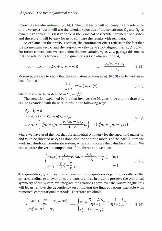
Chapter 8. The hydrodynamical model 117
following (see also Antonelli (2014)). The final result will not contains any referenceto the vortexes, but it will use the angular velocities of the constituent Ωn and Ωp asdynamic variables: this last variable is the principal observable parameter of a glitchand therefore it will be easy for us to compare the results with real data.
As explained in the previous section, the entrainment effect reflects in the fact thatthe momentum vector and the respective velocity are not aligned, i.e. vn 6= pn/mn.For future convenience we can define the new variable vv as vv ≡ pn/mn; this meansthat the relation between all these quantities is (see also section 2.4)
pn = mnvv = mn(vn + εn(vp − vn)) vn =pn/mn − εnvp
1− εn(8.22)
Moreover, it’s easy to verify that the circulation relation in eq. (8.10) can be written inlocal form as:
1x∂
∂ x
x2Ωv
= κn(x) (8.23)
where of course Ωv is defined as Ωv = vθv /x .The condition explained before that involves the Magnus force and the drag one,
can be expanded with these relations in the following way:
fM + fd = 0
κρnez × (vL − vn) = η(vL − vp)
κρnez ×
vθL eθ + v xL ex −
pn/mn − εnvp
1− εneθ
= γ
vθL eθ + v xL ex − vpeθ
(8.24)
where we have used the fact that the azimuthal symmetry for the superfluid makes vnand vp to be directed as eθ ; as done also in the static models of the part II, here wework in cylindrical coordinate system, where x indicates the cylindrical radius. Wecan separate the vector components of the forces and we have:
−ρnvθL +ρn
1− εnpn/mn −
ρnεn
1− εnvp =
γ
κv x
L (ex)
ρnv xL =
γ
κvθL −
γ
κvp (eθ )
(8.25)
The quantities ρX and εX that appear in these equations depend generally on thespherical radius, or anyway on coordinates x and z. In order to preserve the cylindricalsymmetry of the system, we integrate the relations above over the vortex length: thiswill let us remove the dependency on z, making the final equations tractable withnumerical computational methods. Therefore we obtain
−AvθL + Bpn
mn− C vp = Dv x
L
Av xL = DvθL − Dvp
=⇒
vθL =R2 − C/AR2 + 1
vp +1
R2 + 1BA
vv
v xL = eB(vv − vp)
(8.26)

Chapter 8. The hydrodynamical model 118
where the following definitions hold
A=
∫
ρndz B =
∫
ρn
1− εndz C =
∫
ρnεn
1− εndz
D =
∫
γ
kdz R= D/A eB = R
R2 + 1BA
(8.27)
The results just found indicate how a vortex moves under the action of the Magnusand drag forces, because give the velocity vL of the vortex line as a function of thedrag parameters R and eB. The condition of a vortex pinned to the crustal lattice canbe thought as a vortex subjected to a infinite dynamic drag force that therefore actsas a static friction; in other words when γ→ +∞, which implies that D→ +∞, wefind that the vortex line is comovent with the proton fluid because vθL = vp and hasnull component in the radial direction, v x
L = 0. This is precisely what we expect in the“perfect” pinning condition.
We can now consider the continuity equation for the number of vortexes N(x)inside a circle of radius x . This equation can be written, in integral form, as:
dd t
N(x) = −∫
Σ
nvL · dS= −∮
nv xL dl (8.28)
where n represent the vortexes surface density. For the circulation property of asuperfluid (see eq. (8.10)) the above relation becomes
dd t
N(x) =dd t
1κ
2πx pn
mn
=2πκ
xΩv = −nv xL 2πx (8.29)
Now, using eqs. (8.23) and (8.26) we obtain:
Ωv = −1x∂
∂ x
x2Ωv
eB(Ωv −Ωp) = −
2Ωv + x∂
∂ xΩv
eB(Ωv −Ωp) (8.30)
The second equation of motion, needed to complete the system, can be found byconsidering the conservation on angular momentum. This let us to directly encodealso the electromagnetic spin–down (with the variable Text) which is an importantaspect of the rotational properties of neutron stars, and which is not explicitly insertedin eq. (8.16):
dd t
L= −Text (8.31)
Thanks to the consistency relation eq. (8.19) between the entrainment coefficients,and for the definition of vv , the infinitesimal angular momentum can be expressed inthe following way:
dl= x× (ρpvp +ρnvn)dV
= x×
ρp(vp + εp(vn − vp)) +ρn(vn + εn(vp − vn))
dV
= x2
ρp(Ωp + εp(Ωn −Ωp))
+ρnΩv
dVez
(8.32)

Chapter 8. The hydrodynamical model 119
Putting all the pieces together, we can write now the final system in local form:
(ρp − εpρp)Ωp + εnρnΩn = −text(r)−Ψ(r)(ρn − εnρn)Ωn + εpρpΩp = Ψ(r)
(8.33)
where Ψ(r) is the mutual friction term and therefore it’s defined with the eq. (8.30)as Ψ(r) = ρnΩv . The factor text(r) encodes the spin–down torque due to the electro-magnetic emission of the star. We want to adapt here the dipole model of appendix Band therefore we impose that text(r) = βρp(r)Ω3
p. The first equation of the system,taken in absence of entrainment and mutual friction, can be integrated with the factor∫
x2 dV to obtain:IpΩp = −β IpΩ
3p (8.34)
Comparing this equations with the one obtained with the standard magnetic dipoleone can find that
text(r) = βρp(r)Ω3p =
1Ip
R6B2mag
6c3ρp(r)Ω
3p. (8.35)
Considering the local relation εnρn = εpρp, we can solve the initial system for Ωp andΩn:
Ωp = −Ψ(r) + (1− εn)text(r)(1− εn − εp)ρp
Ωn = +Ψ(r) + εp text(r)
(1− εn − εp)ρn
(8.36)
In our simulations we will not consider the differential rotation of the proton fluid;instead we will consider the “protons” (i.e. all the charged components) as a rigidbody. This assumption is justified by the short timescale (less than few seconds) onwhich the ions in the crust are anchored by the superconductive protons in the core:as we want to follow the dynamics of the neutron star with time steps grater thanthis coupling, our model remains consistent and can produce realistic results. Wetherefore integrate the first equation of the system, multiplying both terms by thefactor ρp x2 dV :
Ωp = −1Ip
∫
Ψ(x , z)1− εn − εp
x2 dV +AΩ3p (8.37)
where
A= −R6B2
mag
6c3 I2p
∫
1− εn
1− εn − εpρp x2 dV (8.38)
The dynamical equation for the neutron superfluid must be kept in local form, inorder to follow the movement of the vorticity and therefore the exchange of angularmomentum between the two fluids. As done before, in order to guarantee that the

Chapter 8. The hydrodynamical model 120
angular velocityΩn depends only on the cylindrical radius x and not on the coordinate z,we perform a weighted average over the vortex length for the entrainment coefficients:
εX (x) =
∫
εXρX dz∫
ρX dz(8.39)
In order to simplify the notation, we define also the following quantities:
H(x) = 11− εn − εp
(8.40)
F(x) =εn
1− εn − εp(8.41)
B(x) = eB(1− εn) (8.42)
Q(x) = 1x∂
∂ x
x2
Ωn + εn
Ωp −Ωn
B(x)
Ωp −Ωn
H(x) (8.43)
We can now write the final system of equations that we will use in the followingsimulations:
Ωp = −2πIp
∫ R
0
Q(x)x3
∫ +`(x)
−`(x)ρn dz
d x +AΩ3p
Ωn(x) =Q(x) + βF(x)Ω3p
(8.44)
In case of null entrainment, εn = εp = 0 and eB = B =R/(1+R2) because B = Ain eq. (8.27). Moreover F = 0 and H = 1: the dynamics simplifies in Ωn(x) =Q(x)and Ωp = −
∫
Q(x)x2dV
/Ip − βΩ3p.
8.4 Physical inputs of the model
As our goal is to apply the model just described to simulate a glitch in realistic condi-tions, we must implement the equations using reasonable physical inputs and definethe validity range of all the parameters. The starting point is of course a neutronstar density profile obtained by integrating the TOV equations (see eq. (2.11)) withan equation of state. As done in the previous chapters we will use GM1 and SLy asEoS: by changing the boundary condition of the integration, this approach let us toconstruct a star with specified mass M (and consequently a defined radius R) of whichwe know the density profile ρ(r), as detailed in section 2.2.2. In a fully consistentmodel, the proton fraction xp(r) = ρp(r)/ρ(r) and the entrainment coefficients couldbe obtained directly from the equation of state, because this quantity is a microphysicalproperty of matter. unfortunately, this information is not provided with many of theEoS that can be found in literature (and with the EoS used in this work), so we willconsider the simplified case in which the proton fraction is constant and therefore

Chapter 8. The hydrodynamical model 121
doesn’t depend on the radius r. We introduce the variable Q defined as Q = In/Itot:this approach leads to xp = 1−Q and therefore ρn(r) =Qρ(r) and ρp = (1−Q)ρ(r).As discussed in section 5.2, the results of Zuo et al. (2004) about the proton fractionindicate that Q lies in the range (0.85÷0.95) .
Also the entrainment coefficients are not provided with the EoSs; however, theyhave been calculated recently using different models for the core and the crust of a NS.In particular, Chamel (2012) applied the band theory approach to estimate the valuesof the neutron effective mass m∗n for the typical density range of the inner crust. In thefollowing we will use these values, as we have done in chapter 7 (see fig. 7.1 for a plotof the effective mass versus the barion density, which can be expressed as a function ofthe radius r with eq. (7.1)). It’s important to note that the entrainment is a substantialeffect, as indicated by the ratio m∗n/mn ≈ 10, and not only a small correction: assuggested by the static snowplow model, the vorticity is stored and released in thecrust and therefore this is the part of the star that plays the most important role. Inother words the presence of the entrainment must be carefully considered because itcan affect significantly the dynamics of the system. Regarding the core, Chamel (2006)suggests that the proton effective mass is slightly lower than the bare mass in thecore while we have seen that it’s larger in the crust. This means that the entrainmentparameters will vanish close to the base of the crust and therefore we will consider them∗n = mn in the core. The effective mass is related to the εn coefficient by the equationεn = 1−m∗n/mn; moreover εp = εnρn/ρp, as discussed previously.
8.4.1 Pinning interaction and critical lag
As pointed out in part II, one of the fundamental ingredients of the snowplow modelis the existence of the pinning interaction between the crustal lattice and the neutronvortexes. The model has been developed starting from the ideas of the seminal worksby Alpar et al. (1981) and Anderson et al. (1982), where the authors suggested that thiskind of interaction can be responsible of a storing mechanism for the superfluid angularmomentum; the glitch is therefore a sudden exchange of this angular momentum fromthe superfluid component to the normal one.
In chapter 3 we have presented a mesoscopic approach that has allowed us tomove from the pinning force per single interaction to the pinning force per unit length:as we are considering glitch models, the interaction per unit length plays a crucialrole because it links the microphysics of the vortex–nucleus system to the macroscopicpoint of view required to understand global dynamics. Moreover, our results indicatethat the correct order of magnitude for this last quantity should be 1015 dyn/cm, twoorder of magnitude lower that the forces previously considered. Then, in chapter 5,we have calculated the critical unpinning lag profile ∆Ωcr(x), obtained by equatingthe pinning interaction and the Magnus force (after integration on the vortex length):the fig. 5.5 shows some examples of ∆Ωcr(x) for different configurations. The shapeof this profile, which presents an evident peak located in the crustal region of the star,suggests the storing mechanism for the angular momentum: vortexes are depleted

Chapter 8. The hydrodynamical model 122
in the central region of the star (where ∆Ωcr is low) and packed in a thin sheet justbefore the peak; when the actual lag overcomes the critical value ∆Ωcrmax also thelast barrier is depinned and the recoupling is sudden.
Given its importance, we need to include the pinning also in our hydrodynamicalsimulations. As pointed out previously, we can think of pinning as a static friction,whereas drag is a dynamical one. If we consider the parameter γ in eq. (8.27) andtake γ→ +∞, we obtain B = 0. This means that the pinning condition can be easilymodeled by taking Q(x) = 0 in the stellar regions where vortexes are anchored to thelattice. Of course we discriminate between the two opposite configurations with thecritical lag profile: this means that generally when the actual lag ∆Ω(x) is less than∆Ωcr(x) we are in the pinned condition, while the unpinned condition is given by therelation ∆Ω(x)≥∆Ωcr(x). A different prescription will be used when a glitch starts,as we will discuss later. The term Q(x) in the differential equations must be correctedin the following way:
Q(x) =
0 pinned1x∂
∂ x
x2
Ωn + εn
Ωp −Ωn
B(x)
Ωp −Ωn
H(x) unpinned(8.45)
The critical lag ∆Ωcr(x) is calculated using the same equations of chapter 5 and withthe same hypothesis: we consider that the vortexes are straight and thread the wholestar, and, for the results of chapter 4, we neglect any kind of pinning interaction in thecore. The pinning profile used is the L = 5000,β = 3 case of fig. 3.11.
Generally we will start our simulations with corotating components, which meansthat Ωn(x) = Ωp for every cylindrical radius x . This condition resembles the idealsituation of the star after a glitch that has completely recoupled the two fluids; moreoverin this way we can follow the entire build up of the lag and evaluate the interglitchtime. In the initial condition, of course, vortexes are pinned everywhere; while ∆Ω(x)increase (this is due to the fact that Q(x) = 0 andΩp is subjected to the electromagnetictorque) the inner region of the star switch to the unpinned condition because the lagexcesses the critical values and therefore the components recouple thanks to the termQ(x) 6= 0. These considerations can be useful to understand qualitatively the role ofthe entrainment. If εp = εn = 0, it follows that F(x) = 0 and H(x) = 1 everywhereand therefore the pinned case is equivalent to Ωn = 0. In other words the externaltorque affects only the proton fluid. This is not true when the entrainment is notnull: in this situation, even if Q(x) = 0 (pinned condition), Ωn decreases becausethe external spindown acts partially also on the neutron fluid. This is the same effectdiscussed in section 7.1 and the obvious consequence is that the time needed to buildup a certain lag is greater than the null entrainment case.
Initially we will not consider any kind of repinning and therefore an unpinnedregion remains so until the end of the glitch/simulation. We will discuss later foralternative approaches about this aspect.

Chapter 8. The hydrodynamical model 123
8.4.2 Drag coefficients
As showed by eq. (8.44), all the physical information about the nature of the mutualfriction is encoded in the parameter B that must be discussed carefully. The expressionsin eq. (8.27) indicate that this quantity is a function of the dimensionless term R,which, in turn, is related to the usual drag parameter γ used in other works about thissubject:
B = R1+R2
, R=γ
kρn. (8.46)
It’s clear from this expression that in principle, the parameter B, that is relevantfor us, depends on the position inside the star. As discussed previously, we removethe dependency on the coordinate z by performing an average over that direction(following the vortex–line), but anyway we must handle the dependency on thecylindrical radius because the mutual friction is due to different physical phenomenafor each region of the star. Therefore we need to identify a realistic validity range forthe value of B in the core and in the inner crust of the star, and also to understandwhat happens during a glitch. As we will cover deeply in the next chapter, theinterplay of these different parameter plays a fundamental role in the dynamics ofa glitch, determining the rise time of the event and also the recovery phase: in fact,comparing the system in eq. (8.44) with the dynamical equations of the simple globaltwo component description in eq. (8.1), it’s easy to understand that in our model thetimescale τ of the evolution is linked to B as:
τ≈1− εn
2ΩnB(8.47)
NS Core
In the core of a neutron star, the interaction between the two fluids is due to thescattering of electrons (which are part of the proton fluid) off the neutron superfluidvortexes. From the results of Andersson et al. (2006), this effect couples the compo-nents with a very short timescale (≈ 10 rotational periods, that for the Vela pulsarmeans less that a second). The authors suggest the following expression for the dragcoefficient Bc (the subscript c indicate that this equation is valid in the core region):
Bc = 4× 10⁻⁴
m∗pmp− 1
2mp
m∗p
1/2 xp
0.05
7/6ρ14
1/6 (8.48)
where ρ14 is the total density expressed in units of 1014 g cm−3, xp is the protonfraction (that we consider as a constant) and m∗p is the proton effective mass that isestimated to be in the range m∗p/mp ≈ 0.5÷0.7. The above expression is valid in thecase of a superconductor of type I, but anyway, as pointed out by Sidery and Alpar(2009), the possibility that a fraction of the core is in type II superconducting statemust also be discussed, as this aspect is still unclear. In this case the coupling timescale

Chapter 8. The hydrodynamical model 124
between the two components could be even smaller for the vortex–fluxtube dissipativeinteraction, even if the presence of a pinning effect can significantly change this picturebecause it decouples the two fluid. The results of chapter 4 suggest that the pinningforce per unit length is small if compared to the crustal pinning and therefore wecan neglect this aspect. In this work we will not consider the possibility of a type IIsuperconducting state, even if this is an interesting issue, and, following the sameprescription used by Haskell et al. (2012c), we will adopt the eq. (8.48) to estimatea realistic range for the drag parameter Bc. Equation (8.48) depends weakly on thedensity, which furthermore doesn’t change rapidly in the core of a neutron star: wecan therefore remove this dependency and consider Bc ≈ 1× 10⁻⁴ as a constant forthe whole region. Our simulations will use values for this parameter in the range10−5÷5× 10⁻⁴.
Inner crust
In the inner crust, two different physical processes can be responsible of a mutualfriction between the components, each one with a particular coupling timescale. Aspointed out by Jones (1992), the vortexes can interact with the sound waves inthe lattice: this effect dominates the dissipation when the relative velocity betweenthe vortex line and the lattice is small (vL ≤ 102 cm s−1). The calculation of thedrag coefficient for this process is highly uncertain because it involves a mesoscopicaveraging procedure over the vortex length (similar to the approach used in chapters 3and 4): this lead to a reduction factor of the order of ≈ 10−4. Haskell et al. (2012c)used, for the glitch simulations, a constant parameter Bp ≈ 10−10 to indicate thecoupling due to the lattice phonon oscillations in the inner crust of the star. When therelative velocity between a vortex and a lattice is high, another kind of dissipationcould arise. In this case, for the excitation of Kelvin waves in the vortex, it interactswith the lattice with much shorter timescale respect to the typical one involved in thephononic mutual friction. The results of Epstein and Baym (1992) suggest a value ofBk ≈ 10−3 for the strong drag parameter related to the Kelvin excitations.
To model the dependency of the effective drag on the relative velocity, we constructa profile Bcrust that is a function of the local actual lag ω. We want also to explore theeffect of a strong viscous drag which entangle and block the vortex (it’s therefore apinning–like effect) when the relative velocity with respect to the normal componentfalls below a threshold. In other words we consider a very high value of the dragparameter in order to encode this effect. Thanks to the relation between B and R, i.e.B = R/(1+R2) we can operate in the regime R > 1 and consider a parameter γvsuch that the corresponding B value equals Bp. The net effect on the dynamical modelis therefore the same of a phononic drag, but this approach makes easy to construct atransition function between γv and γk (which correspond to Bk) as a function of thelocal lag ω(x). In this work we consider
Rcrust(x) =γv
κ ⟨ρn(x)⟩exp
§
ln (γk/γv)1+ exp [−q(ω(x)−η |∆Ωcr(x))|]
ª
(8.49)

Chapter 8. The hydrodynamical model 125
10-11
10-10
10-09
10-08
10-07
10-06
10-05
10-04
10-03
10-02
0 0.1 0.2 0.3 0.4 0.5 0.6 0.7 0.8 0.9 1
kelvonic drag
viscous drag
Bcr
ust
ω/ΔΩcr
Figure 8.1: In this figure we plot the dependency of the crustal drag parameter Bcrust overthe lag ω between the two components of the star. For this plot we used eq. (8.49) withγk = 1014 g cm−1 s−1, γv = 1021 g cm−1 s−1 and ⟨ρ⟩ = 5× 10¹³ g cm−3. The parameter η isfixed here to be η= 0.3.
where
q =1S
ln [ln(γv/γk)− 1] (8.50)
and ⟨ρn⟩ is the average of the neutron fluid density over the vortex length. Thisexpression let us to introduce a smooth transition between the two values of theγ parameter which are different for several order of magnitude. The width of thetransition region is S and we fix this value to be 10−4 rad/s, while the transition valueis defined as a fraction η of the local critical lag ∆Ωcr(x) and in the following chapterwe will test also the effect of the parameter η in glitch simulations. From eq. (8.49) wecan easily obtain the resulting Bcrust: the fig. 8.1 shows an example of the dependencyof Bcrust over the lag ω between the two components of the neutron star.
The considerations detailed here define the values of the drag parameter for eachregion of the star. As our model works in cylindrical symmetry, and thanks to the factthat only in the equatorial region the vortexes are full immersed in the crust, we canconsider B(x) = Bcrust(x) for x > Rcore. In the region x < Rcore, the vortexes threadthe core but are also partially immersed in the crust of the star at their extremities;therefore we need to perform an average procedure. Following the expressions ineq. (8.27), we average Rcrust and the corresponding value Rc for the core over thevortex length; then we can calculate with eq. (8.46) the final effective drag B(x) that

Chapter 8. The hydrodynamical model 126
we use in the simulation (see eq. (8.44)).
8.4.3 Triggering a glitch and post–glitch phase
The snowplow model of chapter 5 naturally identifies a trigger mechanism for theglitch: when the actual lag reaches the maximum value of the critical lag profile∆Ωcrmax, all pinning barriers are broken and the vortexes can reach the crust to whichthey transfer their angular momentum. This approach leads of course to a preciselydefined interglitch time, that is the interval required to build up a lag of ∆Ωcrmax. Inchapter 7 this limitation has been overcome with the adoption of a variable trigger, inother words a glitch can happen after a certain time t∗ (or equivalently after a actuallag ω∗) from the previous event. Even if there are many models, the physical natureof this trigger is still unclear, and it’s beyond the scope of this work to investigateabout these aspects. Anyway, triggering a glitch at different lags let us to study theevolution and the resulting observables when the angular momentum available forthe glitch changes: for this hydrodynamic model therefore we will adopt the sameprescription, also to compare the results with the ones of chapter 7. Of course, thequantity ϕ = ω∗/∆Ωcrmax that parameterize the trigger can vary in the range 0÷1,because ∆Ωcrmax represent the maximum lag that can be built up by the star.
When the lag reaches the value ϕ∆Ωcrmax, a glitch is triggered by consideringunpinned all the vortexes in the crust (the part of the crust where the critical lag isbelow the threshold and the whole core are likely to be already depinned) and wechange the drag profile in order to let the two components begin to recouple fast. Thiseffect is achieved only acting on the value Rcrust(x) of eq. (8.49): we only lower thethreshold which determines the shifting between the kelvonic drag and the viscousone, in other words the parameter η is replaced with a new smaller value ηg . Thechange η→ ηg implies that the crust now evolves under the effect of a kelvonic dragBcrust ≈ Bk ≈ 10−3 which is associated to a timescale small enough to produce the riseof the glitch. As explained in the previous section, the recoupling reduces the lagω(x):when its value reaches the threshold ηg∆Ωcr(x), Bcrust ≈ Bp ≈ 10−10 which meansthat the vortexes are entangled and their motion is now decoupled from the crust, asexpected when the vortexes are pinned. In other words our approach permits us toimplement in a simple way the repinning phenomenon after the glitch: the timescalesnow are so long that we can consider the vorticity attached to the lattice and thereforethe star is ready to build up the lag required for another glitch.

CHAPTER 9Results of the dynamical
simulations
The model detailed in chapter 8 has been implemented in a full consistent computercode that can solve the system of differential equations under different physicalcondition. One important aspect of the code is in fact the possibility of changingeasily the inputs of the simulations, allowing us to investigate the influence of a singleparameter on the resulting glitch. We have therefore explored the dependency of theobservable data of this phenomenon with respect to the various drag parameters (inorder to better understand the rise time and the recovery phase) and to the protonfraction of the star. Moreover we have tested different pinning/repinning conditions,together with a parameterized trigger mechanism based on the same prescriptionadopted in chapter 7, in order to reproduce the same results with a dynamical approach.
All the simulations has been built with realistic physical background, startingfrom the density profile of the star: the first step is always the integration of theTOV equations (see eq. (2.11)) with a valid EoS. As the density in the crust of aneutron star changes very rapidly (see fig. 2.5), we need to construct a fairly densespatial grid (with steps d x ≈ 102 cm of the cylindrical radius, in order to maintainthe computations feasible). Furthermore the typical timestep suggested by the valuesof the drag parameters is very small if compared to the interval required to buildup the lag that stores the angular momentum. Taking the Vela Pulsar as example,this interval is ≈ 2.8 yr: this means that use must follow the evolution for about3 year with a timestep of the order of ≈ 10 s (estimated with Bc = 5× 10⁻⁴). Allthese considerations indicate that we are facing a really challenging task from thecomputational point of view: we have therefore developed a highly parallelized andoptimized code that runs in reasonable time and still allows to easily test differentphysical inputs.
The diagram in fig. 9.1 illustrate the scheme of execution of a simulation. Before thetrue evolution code, in the startup block all the physical inputs are correctly evaluated:we prepare the star (obtained by TOV integration) and setup the spatial grids with
127
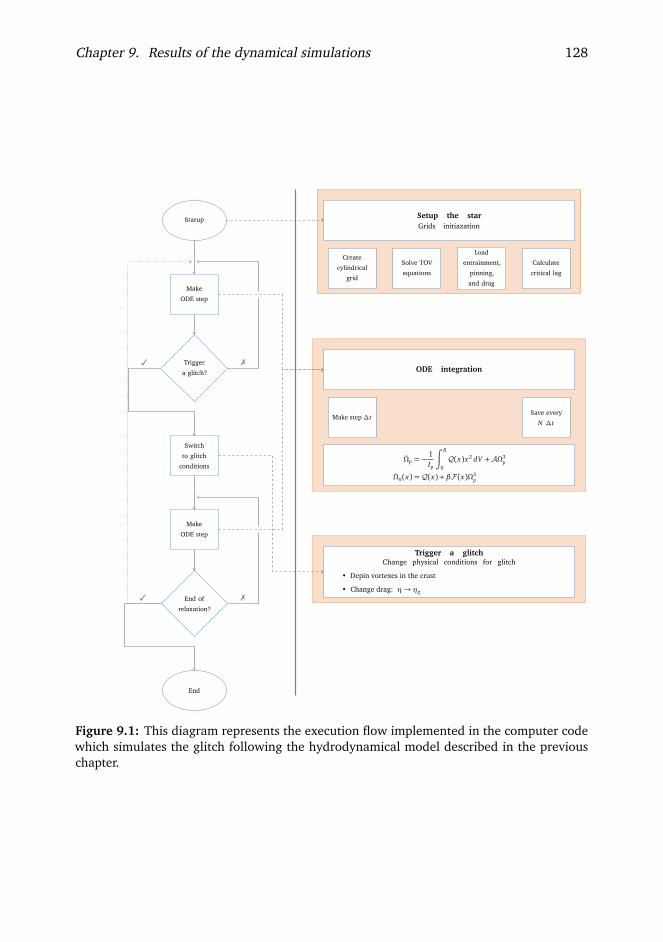
Chapter 9. Results of the dynamical simulations 128
Setup the starGrids initiazation
Create
cylindrical
grid
Solve TOV
equations
Load
entrainment,
pinning,
and drag
Calculate
critical lag
ODE integration
Make step ∆tSave every
N ∆t
Ωp = −1Ip
∫ R
0
Q(x)x2 dV +AΩ3p
Ωn(x) =Q(x) + βF(x)Ω3p
Trigger a glitchChange physical conditions for glitch
• Depin vortexes in the crust
• Change drag: η→ ηg
Starup
Make
ODE step
Trigger
a glitch?
Switch
to glitch
conditions
Make
ODE step
End of
relaxation?
End
73
3 7
Figure 9.1: This diagram represents the execution flow implemented in the computer codewhich simulates the glitch following the hydrodynamical model described in the previouschapter.

Chapter 9. Results of the dynamical simulations 129
precalculated static values, like pinning forces, critical unpinning lag, entrainmentcoefficients and the effective drag profile for the pre–glitch phase. Generally we beginwith corotating components, which means that Ωi ≡ Ωn(x) = Ωp for every cylindricalradius x . After these steps we star integrating the differential equations of eq. (8.44):we use the Runge–Kutta 4th order method with a timestep ∆t to calculate how ourdynamical variables change over time. As described in the previous chapter, we needto consider a set of values for the neutron angular velocity (the star must developdifferential rotation in order to produce a glitch), i.e. Ωni
= Ωn(x i), where the x ipoints are spaced on the grid by an amount d x ≈ 102 cm. On the contrary, for thecharged fluid, we perform an integration at every timestep, in order to consider thecomponent as rigidly rotating and to obtain an observable quantity. The timestep ∆tmust be chosen accordingly to the timescale τ given by the drag forces (following theeq. (8.47)) otherwise the numerical computational error is not controlled.
The pre–glitch phase ends when the glitch conditions (i.e the trigger conditions)are met. Then the event is fired by depinning the part of the crust that is still blockedand by switching to the kelvonic drag: this is obtained by simply substituting theparameter η in eq. (8.49) with a lower value ηg , as explained in section 8.4.2.
9.1 Qualitative analysis of a simulation
We propose the results of simple simulation in order to analyze qualitatively how aglitch is reproduced by our model. In this run we neglect for a moment the entrainment(we will discuss later about the consequences of this effect) and we trigger a glitch onlywhen the actual lag ω reaches the peak of the critical lag profile ∆Ωcrmax. As initialcondition, we take the two fluids as comovent at the typical rotational velocity of theVela pulsar, i.e. Ωi = Ωp = Ωn(x) = 70 rad/s. Moreover we fix the drag coefficientin the core as Bc = 10−4 and we set Bk = 10−3 (the star used is obtained with GM1as EoS and it has mass of 1.3M). The result of the entire simulation is plotted infig. 9.2; in this figure we have reported only the temporal evolution of the angularvelocity Ωp(t) of the charged component. The values are shifted by the quantities t0and Ω0 which represent here the time at the beginning of the glitch and the respectiveangular velocity. We can see that the event happens after ≈ 3 yr from the beginning ofthe simulation.
In the interval before the glitch, the angular velocity decreases regularly for theeffect of the electromagnetic torque (the magnetic field value is taken here to beBmag = 3× 10¹² G). Consequently the lag between the two components increasesbecause, on the contrary, the neutron fluid is decoupled from the magnetic field. Thisis especially true for the inner crust region of the star where the critical lag reachesits maximum. Here the vortexes are pinned and they remain in this condition untilthe triggering of the glitch, thus when the lag overcome the threshold. The inner partof the star instead is involved in a progressive depinning process: starting from theinside and following the steep profile of the ∆Ωcr(x) function, cylindrical shells of the

Chapter 9. Results of the dynamical simulations 130
-4.0⋅10-3
-2.0⋅10-3
0
2.0⋅10-3
4.0⋅10-3
6.0⋅10-3
8.0⋅10-3
1.0⋅10-2
0 2.0⋅107-8.0⋅107 -6.0⋅107 -4.0⋅107 -2.0⋅107
Ω-Ω
0 [r
ad/s
]
t-t0 [s]
02.0⋅10-5
4.0⋅10-5
6.0⋅10-5
8.0⋅10-5
1.0⋅10-4
1.2⋅10-4
0 10 20 30 40 50 60 70 80 90
Figure 9.2: This plot shows how the rotational velocity of the crust (proton component)changes with time in the whole simulation. Points are shifted in order to place the beginningof the glitch at the origin. In the inset the first 90 seconds of the glitch are reported in detail.
neutron component fall in the unpinned condition and therefore begin to recouplewith the charged fluid. The fig. 9.3 shows the typical situation of the star (outer coreand crust) at a given time between two glitches. The shaded region indicates the partwhere the vorticity is still pinned to the lattice, and therefore Q(x) = 0 here (i.e. nodrag force acts here).
Where vortexes are not attached to the crust, the drag coefficients drive theevolution with the timescale given by eq. (8.47). From this expression we can easilyfind the equilibrium lag, that is
∆Ω= −Ωτ= −Ω(1− εn)
2ΩB(9.1)
This condition is reached rapidly in the core, due to the fact that in this region thedrag coefficient that acts between the two fluid is quite strong (Bc ≈ 10−4) . Onthe other hand, in the inner crust a partial fast recoupling (where the lag decreasesconsistently due to the effect of Bk) is followed by a transition to a phononic drag, forthe expression eq. (8.49) used to model the effective mutual friction. This explainthe fact that in fig. 9.3 the profile of the actual lag doesn’t go to zero in the crust:the timescale associated with Bp is too long and the glitch happens before that theequilibrium condition can be reached.

Chapter 9. Results of the dynamical simulations 131
0
2.0⋅10-3
4.0⋅10-3
6.0⋅10-3
8.0⋅10-3
1.0⋅10-2
1.2⋅10-2
6.0⋅105 7.0⋅105 8.0⋅105 9.0⋅105 1.0⋅106 1.1⋅106 1.2⋅106 1.3⋅106 1.4⋅106
ΔΩ
[ra
d/s]
x [cm]
pinned regionΔΩ at t = 1y135.00:00:00 (4.32⋅107 s)
ΔΩcr
Figure 9.3: This plot shows the typical situation at a given time between two glitches. Inparticular we report the lag between the two components and the critical lag profile. Theshaded region represents the part of the star in which vortexes are pinned (decoupled), whilein the other parts the components are coupled thanks to the effect of the mutual friction.
The plot in fig. 9.4 (left part) shows how the vorticity in different zones of thestar are depinned at different time. We plot, together with the value of Ωp, also thevalues of Ωn at some fixed cylindrical radius. Of course the profile of the critical lagmakes it responsible of the fact that at smaller radii the depinning occurs earlier thanin the external positions. This kind of plot is also useful to visualize the effect of theentrainment during the build up of the lag. The left part of the figure is referred to thesimulation described until now, conducted without any form of entrainment. It’s easyto see that where the vorticity is still pinned to the lattice, the corresponding value ofthe neutron angular velocity Ωn doesn’t change. This is not true when the coefficientεn and εp are not null. The right part of fig. 9.4 refers to a simulation in which all theparameters are the same, except for the entrainment that we take into account. Evenin the pinned condition (i.e. before the rapid change of slope) Ωn 6= 0 because theelectromagnetic spindown partially acts also on the superfluid component (the effectis more consistent in the crust; in the core, on the other hand, we take ε = 0). Thisclarifies again the fact that the total time required by the star to build up a fixed lag isbigger when the entrainment plays a role.
When the trigger condition is met (generally when the actual lag at the peakreaches a threshold, for this simulation we take the peak ∆Ωcrmax itself as threshold),the glitch is fired by depinning all the vorticity in the crust and by switching the drag

Chapter 9. Results of the dynamical simulations 132
69.9985
69.9990
69.9995
70.0000
0 0.3 0.6 0.9 1.2
NO entrainment
Ωp
[rad
/s]
t [107 s]
0 0.3 0.6 0.9 1.2
WITH entrainment
t [107 s]
Ωn(0.95 R)Ωn(0.90 R)Ωn(0.85 R)Ωn(0.80 R)Ωn(0.75 R)Ωn(0.70 R)Ωn(0.65 R)Ωn(0.60 R)
Ωp
Figure 9.4: In this figure we show the effect of the entrainment in the model. We plot how Ωpand Ωn (for different cylindrical radii) evolve with time. In the left part (without entrainment)we can see that the Ωn remains constant until the depinnig occurs and this quantity changesrapidly. This effect happens earlier in the core than in the crust due to the shape of the criticallag. In the right part the same quantities are plotted when the entrainment is included in themodel. The considerations above remain valid, but here it’s important to note that also in thepinned case, Ωn is not null, thanks to the presence of the entrainment.
coefficient here to the value Bk (i.e. to strong kelvonic mutual friction), thanks to thesubstitution η→ ηg . This means that a bulk of superfluidity stars recoupling at thesame time, and with a very fast timescale. The values of Q(x) is strongly affectedand the integral in eq. (8.44) produces a fast positive variation of Ωp, because Ωn > 0(the recoupling is so strong that it overcomes the electromagnetic torque). This is the“rise” phase of the glitch (dominated by the strongest among the drag parameter, i.e.Bk) that corresponds to the first ≈ 5s in the left plot of fig. 9.5. In the same plot wecan see that Ωn decreases in the crust and this reduces the lag, bringing the systemtowards the condition of equilibrium.
Looking at the profileΩp(t), it’s noteworthy that the rise of the glitch is immediatelyfollowed by a short term recovery that happens with a timescale of ≈ 50s: afterreaching the maximum∆Ωgl = Ωp(tmax)−Ωp(0) (in this simulation∆Ωgl = 10−4 rad/s;here and in the following we consider with t = 0 the beginning of the glitch), thederivative Ωp changes sign and therefore the proton angular velocity is reduced, untilthe “recovery” effect ends. This behavior is explained if we look at the critical lag inthe core region. In fact, due to the rapid spin–up of the whole star and the low values

Chapter 9. Results of the dynamical simulations 133
10-6
10-5
10-4
10-3
10-2
10-1
0 20 40 60 80 100
Ω(t
) - Ω
0 [r
ad/s
]
t-t0 [s]
ΩpΩn(xmax)
-5
0
5
10
15
9 10 11 12 13ΔΩ
[10
-4 r
ad/s
]
x [105 cm]
Ωn - Ωp at (t0 + 5s)ΔΩcr
Figure 9.5: The left plot shows the first 100s after the beginning of a glitch. We can see theinitial rise phase (due to the effect of Bk; it ends when ∆Ωp reaches its maximum) and therecovery phase in which Ωp < 0 with absolute value granter than the pre–glitch one. In theright figure we plot the critical lag profile and the actual lag at the end of the rise. We can seethat in the core the lag has changed its sign: this explains the recovery effect due to the coredrag Bc (see eq. (8.44)).
of ∆Ωcr here, the actual lag Ωn −Ωp changes its sign in eq. (8.44), as we can see infig. 9.5 (right plot, shaded region), referred to a time t = 5 s after the beginning ofthe glitch. The flat profile of ∆Ωcr for x < Rcore indicates that the effect is consistentbecause the whole region is involved at the same time, even if the actual lag is small.
As shown, this phase is dominated by the recoupling of the core (subsequent ofthe rapid spin–up) and therefore the coupling parameter is Bc which is associatedto a timescale one order of magnitude larger than the one imposed by Bk. Theinterplay of these two parameters strongly affects the dynamics of the phenomenon:the kelvonic drag takes part firstly and defines mainly the maximum jump ∆Ωgl ofthe glitch (and how long does it take to reach this value), while the mutual frictionin the core of the neutron star fixes how fast Ωp(t) reaches its final value. This valueis also dependent on the value of the parameter ηg which defines when the repinnigcondition is reached. The dependency of the resulting Ωp(t) on these parameters willbe explored quantitatively in the next section.

Chapter 9. Results of the dynamical simulations 134
9.2 Parameter study
In the previous section we have seen, from a qualitative point of view, that the timeevolution of a glitch is controlled by some parameters of our model. Here we want toexplore deeply this aspect, giving some quantitative results obtained with simulationsconducted with different conditions. In order to simplify the following discussion, wedefine now some relevant quantities. Unless otherwise specified, we consider the glitchoccurring at time t = 0 (time when the trigger is fired), and the corresponding angularvelocity of the charged component is Ω0. The variable tgl represents the time passedfrom the beginning of the simulation to the glitch itself (at the initial condition thetwo fluids are comovent), and corresponds roughly to the interglitch time. Generallywe plot the quantity ∆Ωp(t) = (Ωp(t)−Ω0), which evolves with time and representthe principal observable quantity of the event. The maximum absolute value reachedby ∆Ωp(t) is the actual jump size that we identify with the term ∆Ωgl; moreover thiscondition is reached after a time tmax (the risetime) from the beginning.
In all the simulations we take into account also the entrainment effect: thismeans that the coefficients εp and εn are not zero (the profile used is the one plottedin fig. 7.1, see eq. (8.39) for the averaging procedure over the vortex length). Asdiscussed previously, with the entrainment the time required to build up a fixed lagis larger by a factor of the order of εn, i.e. ≈ 10. We have verified that our modelbehaves as expected about this aspect: we have done two identical simulations exceptfor the εX coefficients. The glitch is always triggered when the actual lag reaches thesame fraction ϕ = 0.3 of the critical lag: in one case we find tgl = 2.4× 10⁷ s, whilewe obtain tgl = 1.9× 10⁸ s when the entrainment is switched on (the other parametersused here are: GM1 EoS, M = 1.3M, Q = 0.95, Bmag = 3.1× 10¹² G, Bc = 10−4 andBk = 10−3).
The entrainment affects significantly also the risetime of the glitch. In fact, fromthe eq. (8.47), we know that the timescale of the evolution is controlled, of course, bythe mutual friction (with the B parameter), but it depends also on the εn coefficient,which corrects the final values. This is especially true for the crust region because hereεn ≈ −10 (as discussed previously, we take the entrainment null in the core): in otherwords, this slows down the effect of Bk which acts here. In particular the value oftmax increases when the entrainment is switched on by a factor ≈Ým∗n. Referring to thesimulation described in the previous section (where εX = 0), we can see that a kelvonicdrag Bk = 10−3 produces a risetime tmax ≈ τ = 7 s; this result is in agreement withthe analysis of Dodson et al. (2002, 2007) in which an upper limit for this quantity(al least for the Vela pulsar) is set to 40s. In order to satisfy this constraint with theentrainment, we have to increase the value of the parameter Bk of roughly one orderof magnitude, because 1− εn ≈ 10. This is the first parameter that we study here,letting it vary in the range 5× 10⁻³÷5× 10⁻², for the reasons discussed. We havetaken a 1.3 M GM1 star, with Q = 0.95; the pinning profile is the L = 5000,β = 3calculated in chapter 3 and we have used the prescription for the drag coefficient ofsection 8.4.2 (η = 0.6,ηg = 0.2), keeping Bc fixed at 10−4 for all runs while changing

Chapter 9. Results of the dynamical simulations 135
2.0⋅10-4
2.5⋅10-4
3.0⋅10-4
3.5⋅10-4
4.0⋅10-4
4.5⋅10-4
0.1 1 10
ΔΩ
p [r
ad/s
]
t [s]
(1)(2)(3)(4)(5)(6)(7)(8)(9)
(10)
0 1 2 3 4 5 6
Bk/10-2
(1)(2)(3)(4)(5)(6)
(7)(8) (9) (10)
Figure 9.6: In this figure we plot the effect of the kelvonic drag parameter Bk over ∆Ωp(t).We explore the range 5× 10⁻³÷5× 10⁻² and in the right part we plot the value of Bk and thecorresponding maximal glitch size ∆Ωgl. The filled dot indicates the best benchmark for thisparameter: this value will be used also in the following simulations.
Bk; the glitch is trigger when the lag ω= |Ω|t reaches the typical value for the Velapulsar, i.e. 8.04× 10⁻³ rad/s. The results of these simulations are showed in fig. 9.6.In the left part we plot how the rotational velocity of the crust changes in the first60 seconds after the glitch, while in the right part the maximum jump size ∆Ωgl isplotted against the corresponding Bk value. As expected, increasing Bk result in areduction of the rise time tmax. This means that the angular momentum stored by thesuperfluid is released to the crust in a shorter time and therefore the peak reachedby the proton rotational velocity, i.e. ∆Ωgl, is bigger because a smaller fraction ofthe core superfluid has begun to recouple. In the range of Bk tested, we obtain themaximum jump of ≈ 4× 10⁻⁴ rad/s when Bk = 5× 10⁻², and the corresponding risetime observed is less than 10 seconds, well below the constraint of 40 s. A high valueof the kelvonic drag parameter is correlated to a more evident recovery effect: aninitially larger glitch rapidly relaxes to a lower spin rate than that of a glitch involvinga weaker drag parameter in which the timescales of Bk and Bc partially overlap.
In fig. 9.7 we keep Bk = 10−2 fixed and we change the drag parameter Bc for thecore region in the range 10−5÷5× 10⁻⁴ (all other parameter are the same used infig. 9.6). The dependency of the glitch size to this parameter is inverted with respectto the kelvonic mutual friction: increasing Bc results in a smaller jump because theangular momentum transfer is suppressed by the strong recovery, as shown by the

Chapter 9. Results of the dynamical simulations 136
1.5⋅10-4
2.0⋅10-4
2.5⋅10-4
3.0⋅10-4
3.5⋅10-4
4.0⋅10-4
1 10 100 1000
ΔΩ
p [r
ad/s
]
t [s]
(1)(2)(3)(4)(5)(6)(7)(8)(9)
0 1 2 3 4 5
Bc/10-4
(1)(2)
(3)(4)(5)(6)(7)
(8)(9)
(1)
(2)(3)(4)(5)(6)(7) (8) (9)
Figure 9.7: In this figure we plot the effect of the core drag parameter Bc over ∆Ωp(t). Weexplore the range 1× 10⁻⁵÷5× 10⁻⁴ and in the right part we plot the value of Bc and thecorresponding maximal glitch size ∆Ωgl with circles and ∆Ω60 with squares. This last quantitycorresponds to the jump size extracted after 60 s form the beginning of the glitch and will beused later. The filled dots indicate the best benchmark for this parameter: this value will beused also in the following simulations.
right plot of the figure. Nevertheless we can see that the main effect of Bc regards thepost–jump behavior in particular it determines how fast the rotational velocity of thecrust reaches its “final” value, as we can see in the plot (in this context, with the term“final” value we identify the residual jump ∆Ωp measured when the stellar regions arefully relaxed (see eq. (9.1)) or fully repinned).
In the two sets of simulations covered until now, we have only acted on the dragparameters Bc and Bk. As explained, these values control the timescales of the differentphases of a glitch, but it’s clear from the derivation of the chapter 8 that they don’taffect the total angular momentum stored by the superfluid neutron vortexes beforethe glitch and released after to the charged component. In other words this means thatthe jump ∆Ωp observed when the crust and the core are fully relaxed (i.e when Bcand Bk have done their jobs) is the same for all runs, as we can see in the previouslydiscussed plots. With the global two component model, covered at the beginning ofchapter 8 and in appendix B, we can see that this aspect is controlled, as expected,by the parameter Q, that is the ratio between the moment of inertia of the superfluidconstituent and the total moment of inertia of the star(see eq. (B.10)). We want nowto test if our dynamical model shows the same behavior, i.e. the final jump is bigger

Chapter 9. Results of the dynamical simulations 137
2.5⋅10-6
3.0⋅10-6
3.5⋅10-6
4.0⋅10-6
4.5⋅10-6
5.0⋅10-6
5.5⋅10-6
6.0⋅10-6
0 50 100 150 200
ΔΩ
p/Ω
0
t [s]
Q = 0.850 Q = 0.900 Q = 0.950 Q = 0.975
2.80⋅10-6
2.85⋅10-6
2.90⋅10-6
2.95⋅10-63.00⋅10-6
3.05⋅10-6
3.10⋅10-6
3.15⋅10-6
3.20⋅10-6
160 165 170 175 180 185 190 195 200
Figure 9.8: This plot shows the dependency of the glitch size on the neutron fraction valueQ. This parameter affects the quantity ∆Ωgl but also the residual jump size at the end of therecovery, as we can see in the small figure.
when we increase the proton fraction. The plot in fig. 9.8 reports the dependencyof the residual jump with respect to the ratio Q = In/Itot (see appendix B for detailsabout the relation between the healing parameter of the global two component modeland the proton fraction of the star).
In the runs reported in this section we have kept fixed ηg = 0.2. Of course thisparameter affects the recovery phase of the glitch: when the lag falls below thethreshold defined by ηg the vortexes behave like they are repinned to the lattice andthe motion of the two components is therefore completely decoupled. This means that∆Ωp doesn’t change anymore (the effect given by the secular slowdown is too small tobe visible on the timescales considered here), as we can see in fig. 9.9. In this plot wechange the value of ηg while the other parameters are fixed at their best benchmarksused also previously (Bk = 10−2, Bc = 10−4, Q = 0.95, with GM1 as equation of stateand M = 1.3M). As expected, the flat curve condition is reached before when ηg isincreased. For ηg = 0.2 we can see that the vortexes are repinned after ≈ 60s.
In the following we will use this value, ηg = 0.2, for the simulations. This choiceis reasonable if we take into account the observative data of the Vela glitches. Dodsonet al. (2002, 2007) provide a fit of the residuals for two giant glitches of this pulsar,namely the event in 2000 and the one in 2004, giving also an estimate for a very short(of the order of a minute) timescale term of the evolution (no timing analysis hasn’tbeen yet published for the following glitches of Vela). We plot these two fits in fig. 9.10,

Chapter 9. Results of the dynamical simulations 138
0
1.0⋅10-4
2.0⋅10-4
3.0⋅10-4
4.0⋅10-4
5.0⋅10-4
0 20 40 60 80 100 120 140
ΔΩ
p [r
ad/s
]
t [s]
(1)(2)(3)(4)(5)(6)
0 0.1 0.2 0.3 0.4 0.5
ηg
(1)(2) (3)(4)
(5) (6)
Figure 9.9: In this figure we change the value of the parameter ηg (see section 8.4.2 fordetails) and we plot the curves ∆Ωp(t) for the first 150 s form the beginning of the glitch. Inthe right part we plot the value of ηg and the corresponding value of ∆Ω60 (glitch size after60 s). The dot highlighted corresponds to the value of ηg that we take as benchmark for thenext simulations.
together with the output of our simulation with ηg = 0.2 (as done before, Bk = 10−2,Bc = 10−4, Q = 0.95, with GM1 as equation of state and M = 1.3M). In this figurewe report the residuals, i.e. the change in rotational frequency after removing alsothe pre–glitch spin–down. The two events seem to be very different in the first twominutes from the beginning: in the 2000 glitch the change in ν is less than 0.1% whilethe situation is different for the other glitch, as we can see in fig. 9.10 (but we shouldtake into account that the 2004 fit is less significant due to the quality of data (Dodsonet al., 2007)). Anyway it’s important to underline the fact that observational datadon’t show any risetime (Ωp is always negative) and the glitch is therefore consideredas an “instantaneous” step: the upper limit for this phase is 40 s. In other words thereis an unobserved window of ∼ 1 min in which ∆Ωp(t) reaches its maximum and it’salready decreasing when we begin to record data. For this reason we are interested inthe quantity ∆Ω60 which is the jump size extracted after 60 s from the beginning ofthe glitch, i.e. ∆Ω60 = Ωp(t = 60s)−Ω0. In this perspective, the choice ηg = 0.2 isreasonable as it allow us to simulate an intermediate glitch between the two events ofVela considered, and to fit well the 2000 one if we shift the curve (we consider theglitch as starting at t = −60s, see the fig. 9.10).
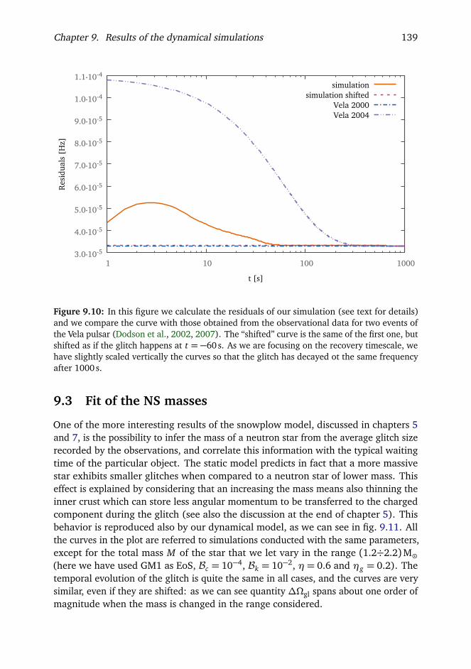
Chapter 9. Results of the dynamical simulations 139
3.0⋅10-5
4.0⋅10-5
5.0⋅10-5
6.0⋅10-5
7.0⋅10-5
8.0⋅10-5
9.0⋅10-5
1.0⋅10-4
1.1⋅10-4
1 10 100 1000
Res
idua
ls [
Hz]
t [s]
simulationsimulation shifted
Vela 2000Vela 2004
Figure 9.10: In this figure we calculate the residuals of our simulation (see text for details)and we compare the curve with those obtained from the observational data for two events ofthe Vela pulsar (Dodson et al., 2002, 2007). The “shifted” curve is the same of the first one, butshifted as if the glitch happens at t = −60 s. As we are focusing on the recovery timescale, wehave slightly scaled vertically the curves so that the glitch has decayed ot the same frequencyafter 1000s.
9.3 Fit of the NS masses
One of the more interesting results of the snowplow model, discussed in chapters 5and 7, is the possibility to infer the mass of a neutron star from the average glitch sizerecorded by the observations, and correlate this information with the typical waitingtime of the particular object. The static model predicts in fact that a more massivestar exhibits smaller glitches when compared to a neutron star of lower mass. Thiseffect is explained by considering that an increasing the mass means also thinning theinner crust which can store less angular momentum to be transferred to the chargedcomponent during the glitch (see also the discussion at the end of chapter 5). Thisbehavior is reproduced also by our dynamical model, as we can see in fig. 9.11. Allthe curves in the plot are referred to simulations conducted with the same parameters,except for the total mass M of the star that we let vary in the range (1.2÷2.2)M(here we have used GM1 as EoS, Bc = 10−4, Bk = 10−2, η= 0.6 and ηg = 0.2). Thetemporal evolution of the glitch is quite the same in all cases, and the curves are verysimilar, even if they are shifted: as we can see quantity ∆Ωgl spans about one order ofmagnitude when the mass is changed in the range considered.

Chapter 9. Results of the dynamical simulations 140
0
5.0⋅10-5
1.0⋅10-4
1.5⋅10-4
2.0⋅10-4
2.5⋅10-4
3.0⋅10-4
3.5⋅10-4
4.0⋅10-4
4.5⋅10-4
0 10 20 30 40 50 60 70 80
ΔΩ
p [r
ad/s
]
t [s]
(1)(2)(3)(4)(5)(6)(7)
1 1.2 1.4 1.6 1.8 2 2.2 2.4
M [MΟ•]
(1)
(2)(3)
(4)
(5)
(6)(7)
Figure 9.11: This figure shows the effect of the mass on the glitch. We simulate differentglitches when all the parameters are kept fixed at their best benchmarks except for the massM of the star. We can see that a lower mass star is associated to a bigger glitch, as expectedfrom the results of the snowplow model of chapters 5 and 7. On the right part we plot thevalue of M and the corresponding ∆Ω60 (glitch size after 60 s).
In the snowplow model, a similar effect on ∆Ωgl is played also by the parameterYgl, as discussed in section 7.2. This quantity encodes, in the static model, the fractionof superfluid matter coupled to the normal one at the glitch: this means that somehowYgl determines also the jump size, because in the limiting case of Ygl = 0 all the angularmomentum stored is transferred uniquely to the crust, producing the maximal glitch.The inverse dependency of these two quantities is plotted in fig. 7.3. The degeneracyof M and Ygl over the glitch size has been removed in the snowplow model by fixingthe parameter Ygl in order to obtain a mass for the Vela pulsar of 1.3M. Then wehave used the same value of Ygl to infer the mass of all other frequent glitchers: thecalculated masses are reported in table 7.1. Moreover we have discussed about therelationship, showed by the observational data, that involves ∆Ωgl and the averagelag ω = |Ωp| ⟨tgl⟩ built by the star in the time between two consecutive events (seefig. 7.15).
Now we want to test if these results are also compatible with the dynamical modelproposed here. We consider the six most frequent glitchers of table 2.2 and, for eachcase, we construct the respective star that will be used in the simulation: we useGM1 as EoS and for the mass M we take initially the total mass obtained by thefitting procedure of the snowplow model. Then we start the simulation detailed in

Chapter 9. Results of the dynamical simulations 141
0
5.0⋅10-5
1.0⋅10-4
1.5⋅10-4
2.0⋅10-4
2.5⋅10-4
3.0⋅10-4
3.5⋅10-4
4.0⋅10-4
0 10 20 30 40 50 60 70 80
ΔΩ
p [r
ad/s
]
t [s]
(1)(2)(3)(4)(5)(6)
0 0.002 0.004 0.006 0.008 0.01 0.012
ω* [rad/s]
(1)
(2)(3) (4) (5) (6)
Figure 9.12: In this plot we change the value of the triggering parameter ω∗, i.e. the lag builtby the two components at which the glitch is triggered when reached. All other parametersare kept fixed. This plot is analogous to those obtained with the snowplow model in chapter 7.On the right part we plot the value of ω∗ and the corresponding ∆Ω60 (glitch size after 60 s).
this chapter, and we use the prescription of section 8.4.3 to fire a glitch. This meansthat we start a glitch when the raw lag ω build by the star reaches the critical valueω∗ which corresponds to the observational average lag for this particular pulsar (infig. 9.12 we show the glitches obtained by changing the value of the triggering lag,while all other parameters are kept fixed; we can see that qualitatively the relationshipbetween ∆Ωgl and ω is in agreement with the behavior studied with the snowplowmodel, e.g. see figs. 7.3 and 7.4). The ultimate goal is to compare the jump size thatcomes from the simulation with the observational value of the extremal event.
In the dynamical approach, the parameter Ygl doesn’t exists, but its role is playerhere by the drag coefficients Bk and Bc because they controls the timescale, andtherefore also the amount, of the coupling between the superfluid and the normalcomponent of the star. In other words, the jump size is not affected only by the totalmass, but it is also affected by these parameters, as Ygl does in the static model. Asdiscussed previously, the figs. 9.6 and 9.7 show quantitatively these effects. Moreoverwe have another source of degeneracy which comes from the parameter η of theeffective drag in the crust before the glitch (η represent the fraction of the critical lagat which we have the transition to the viscous drag; see section 8.4.2). In fig. 9.13 wereports the results of the simulations performed by changing only the value of η, whilekeeping fixed all other parameters. We can see that the resulting effect is opposed

Chapter 9. Results of the dynamical simulations 142
0
5.0⋅10-5
1.0⋅10-4
1.5⋅10-4
2.0⋅10-4
2.5⋅10-4
3.0⋅10-4
3.5⋅10-4
4.0⋅10-4
4.5⋅10-4
0 10 20 30 40 50 60 70 80
ΔΩ
p [r
ad/s
]
t [s]
(1)(2)(3)(4)(5)(6)(7)
0 0.2 0.4 0.6 0.8 1
η
(1)(2)
(3)
(4)
(5)
(6)(7)
Figure 9.13: With this figure we analyze the effect of the last parameter of the model, η,which control the transition from the kelvonic drag to the viscous one in the crust. As expecteda higher value of η produces a bigger glitch, as shown by the right part where η is plottedagainst ∆Ω60.
to the one obtained by changing the mass of the star: by increasing η we increasethe amount of angular momentum stored by the superfluid in vortexes between twoglitches and ready to be transferred suddenly to the crust (on the other hand, the glitchsize has an inverse dependency on the mass M , as showed before; this degeneracy issimilar to the one discussed in the snowplow model of chapter 7 between M and Ygl).
Based on the results in figs. 9.6 and 9.7 we decide to fix the kelvonic drag parameterto be Bk = 10−2, and for the core coefficient we take Bc = 10−4 as this is the bestbenchmark (see eq. (8.48)). This reasonable choice, together with ηg = 0.2 guaranteesthat the rise time of the glitches remains below the constraint of ∼ 40–60s, whilethe recovery timescale is in agreement with the observable data for the Vela pulsar(Dodson et al., 2002, 2007). In order to fix the value for η we adopt precisely thesame strategy proposed for the static model approach: we consider initially the Velapulsar B0833–45 and we change η until we can reproduce (with the choice of theother parameters detailed above) the maximum glitch size recorded by observations(η= 0.6). With the procedure described now, all of the free parameters of the modelare fixed, except for the mass M and the lag ω = |Ω|t at the glitch. Of course ω comesfrom the observational data (table 2.2, reported also in table 9.1), while for M wefollow the same approach used in chapter 7. As explained before, we are focusedon the quantity ∆Ω60 (jump size after 60 s from the beginning of the glitch) that we

Chapter 9. Results of the dynamical simulations 143
0
1.0⋅10-4
2.0⋅10-4
3.0⋅10-4
4.0⋅10-4
5.0⋅10-4
0 20 40 60 80
ΔΩ
[ra
d/s]
t [s]
J0537-6910B0833-45B1046-58B1338-62
J0631+1036B1737-30
Figure 9.14: In this figure we plot the ∆Ωp(t) curves of our best fits for the six pulsarsconsidered (for GM1; the corresponding plot for SLy is very similar). The triangles indicatethe observational values that we fit with the procedure described (see also table 9.1).
compare with the maximum observed ∆Ωgl for each particular star: for every pulsarwe slightly change the mass M until ∆Ω60 matches the biggest glitch.
The inferred masses obtained with this approach are reported in table 9.1. Theprocedure has been applied also for the SLy equation of state, with the same choicesfor the pinning profile (L = 5000, β = 3 of chapter 3), neutron fraction (Q = 0.95)and drag forces: Bc = 10−4, Bk = 10−2,ηg = 0.2. On the contrary, the parameter ηhas been fixed in order to reproduce ∆Ωglmax
= 2.17× 10⁻⁴ rad/s, which is the Velamaximum glitch size, with a 1.3M star; the simulations indicate η= 0.9.
In figs. 9.15 and 9.16 and table 9.1 we give the results for GM1 and SLy togetherwith the ones obtained with the snowplow model in chapter 7, for a comparison. Thefig. 9.14 summarizes the simulations that are our best fits for the pulsar consideredwith GM1 as equation of state. The triangles represent the observational values takenas a reference for each star, positioned at 60 s as we extract the quantity ∆Ω60 fromthe calculated curves.
In fig. 9.17 we replot the time evolution of our best fits of table 9.1 and fig. 9.14(these are the simulations from which we extract the ∆Ω60 value to be comparedwith the observational data), for GM1 EoS. As done before, we plot, for each pulsar,the curve ∆Ωp(t) = Ωp(t)−Ωp(0), and also the equivalent quantity ∆Ωn(t) for theneutron component. This quantity is obtained as ∆Ωn(t) = ⟨Ωn(t)⟩ −Ωp(0), where⟨Ωn⟩ is a weighted average of the angular velocity of neutrons. In our model we have

Chapter 9. Results of the dynamical simulations 144
Table 9.1: This table summarizes the results of the fitting procedure for both SLy and GM1.For each pulsar, the reported mass M is the value of this parameter which fits better theobservational data, comparing the result with the one obtained in chapter 7 with the snowplowmodel. We report also the average lag ω = |Ω| ⟨tgl⟩ (see table 7.2) of the particular pulsarused to trigger the glitch in the simulations and the maximum observed glitch size taken asreference to infer the mass of the pulsar.
Pulsar name ω ∆ΩglmaxSLy GM1
[rad/s] [rad/s] Snowplow Dyn. model Snowplow Dyn. model10−4 10−5 [M] [M] [M] [M]
J0537-6910 131.00 26.54 1.22 1.20 1.20 1.20J0631+1036 2.70 7.16 2.04 1.80 2.33 1.85B0833-45 80.44 21.70 1.30 1.30 1.30 1.30B1046-58 37.96 15.46 1.52 1.45 1.61 1.45B1338-62 11.86 10.00 1.81 1.70 1.96 1.75B1737-30 1.92 2.76 > 2.04 2.00 > 2.36 2.30
1
1.2
1.4
1.6
1.8
2
2.2
2.4
10-4 10-3 10-2 10-1
M [
MΟ•]
ω [rad/s]
J0537-6910
J0631+1036
B0833-45
B1046-58
B1338-62
B1737-30
Figure 9.15: We plot here the inferred mass M (with SLy, obtained with the fitting proceduredescribed) of the considered glitchers versus the average lag ω.

Chapter 9. Results of the dynamical simulations 145
1
1.2
1.4
1.6
1.8
2
2.2
2.4
10-4 10-3 10-2 10-1
M [
MΟ•]
ω [rad/s]
J0537-6910
J0631+1036
B0833-45
B1046-58
B1338-62
B1737-30
Figure 9.16: We plot here the inferred mass M (with GM1, obtained with the fitting proceduredescribed) of the considered glitchers versus the average lag ω.
considered Ωn as a function of the cylindrical radius, and therefore we must define amean quantity to compare it with the angular velocity of the crust (proton fluid). Thenatural way to accomplish this task is to take into account the total angular momentumLn stored by the superfluid and therefore we define
⟨Ωn(t)⟩=Ln
In=
4πIn
∫ Ric
0
x3Ωn(x , t)
∫ `(x)/2
0
ρn(x , z) dz
d x (9.2)
where Ric is the radius of the inner/outer crust interface and `(x) = 2q
R2ic − x2 is the
length of a vortex for which x is its distance from the rotational axis. Thanks to thedefinition in eq. (9.2) we obtain the “equivalent” global two component model andthe plots in fig. 9.17 show an interesting point. The simulations in which the protonfluid velocity temporarily overcomes the neutron one, are also the ones that showa marked overshoot phase and therefore an evident recovery effect, indicating thatthese two aspects are strictly linked, as expected. This behavior is present in the firstthree plots of the figure, but not in the last three glitches where the rise phase is notstrong enough to accelerate the proton component to a velocity bigger than ⟨Ωn⟩ andtherefore there is no velocity inversion. This behavior seems again to be controlled bythe lagω built by the star between glitches (as also showed by fig. 9.12) and therefore,for our analysis, by the mass of the pulsar: this suggests that the shape of the ∆Ωp(t)profile could be another indicator of the parameter M .

Chapter 9. Results of the dynamical simulations 146
0
1.0⋅10-4
2.0⋅10-4
3.0⋅10-4
4.0⋅10-4 J0537-6910
ΔΩ
[ra
d/s]
B0833-45 B1046-58 pn
0
1.0⋅10-4
2.0⋅10-4
3.0⋅10-4
4.0⋅10-4
0 30 60 90
B1338-62
ΔΩ
[ra
d/s]
t [s]
0 30 60 90
J0631+1036
t [s]
0 30 60 90
B1737-30
t [s]
Figure 9.17: For each of the pulsar that we take into account, we plot here the time evolutionof the simulation which fits better the observational data (for GM1; the corresponding plotsfor SLy are very similar). We plot the ∆Ωp(t) curve and also ∆Ωn(t), calculated from theweighted average of the rotational velocity of the neutron fluid, as described in eq. (9.2).
9.4 Conclusions
The results are in good agreement with those obtained with the snowplow modeland thus the same considerations done at the end of chapter 7 are valid. We havefound the same dependency between the mass of the pulsar and the glitching strength(fig. 9.11); moreover the strong correlation between M and ω of figs. 7.18 and 7.19is recorded also with the dynamical model described here, as we can clearly see infigs. 9.15 and 9.16. This fact indicates that also this approach (like the static one)provides a unique explanation for both the small and the large glitchers, covering therange spanned by the observational data. As a consequence, the correlation betweenmass and lag can be understood by the same qualitative considerations reported insection 7.4. It’s noteworthy the fact that with the dynamical approach all the NSsconsidered are fitted well, also the object B1737–30: the snowplow model in this casepredicts a mass above the maximum allowed Mmax for both the EoSs considered (inother words, the static model predicts jumps significantly larger than those observed).On the contrary, with the approach presented in this chapter, the glitching behavior ofthis star is explained consistently in the same way as for the other pulsars (in fact theinferred mass is slightly below the Mmax limit, see table 9.1): this confirms the validityof this model in encompassing both large and non–large glitchers. Moreover we must

Chapter 9. Results of the dynamical simulations 147
point out that both models (static and dynamic) provide an upper bound for the massof a NS, as they fit its maximum glitch: therefore it’s always possible that in the futurea new larger event lowers the inferred mass. This is especially true for B1737–30 as itspins down slower than the other stars and maybe we have not yet observed it longenough: with a slightly larger glitch and therefore a slightly lower mass required inthe simulations, the data would show globally an even better correlation between Mand ω.
While the results presented here are in agreement with the snowplow model, thisdynamical model has many advantages over the static approach, because it allowsus to study the full temporal evolution of the interglitch phase and also the rise andrecovery of the jump. Moreover we have shown that it’s easy to take into accountall the required microphysical inputs, like pinning forces and drag interactions, andtherefore building a more realistic model. In this work we have focused on the shortterm recovery which is due to the fast recoupling of the components of the star: infig. 9.10 we have compared our results with the observed glitches of the Vela pulsar(2000 and 2004). Our simulation shows an intermediate behavior between the twocurves taken as reference that are quite different in the first two minutes. In lookingat these data we must always take into account that the upper limit for the rise of aglitch is of ∼ 60 s. This indicates that the observational data available at the momentlack of very important information about, at least, the first minute of a glitch, whichis a complex phase as it contains the rise, the true maximum ∆Ωgl reached and alsoa fast recovery. For this reason generally we have chosen to fit the observed ∆Ωglvalues with the jump size extracted after 60 s, for a more realistic comparison. Wehave also shown that by shifting our simulation by 60 s we can fit well the Vela 2000curve (which is of better quality). It’s clear now that having a precise observation ofthe first seconds of a glitch is really important as it would give great hints on the dragcoefficients and therefore on the whole process.
Even if we have dealt with the fast recovery, of course the longer timescalessuggested by the observational data can be explained by introducing other dragparameters to encode the fact that different zones of the star recouple at differenttimes. The understanding of these aspects it’s a very interesting task that we will tacklein a future work.

Conclusions and future directions
In this thesis we have faced the problem of pulsar glitches from different perspectives.This approach has been suggested by the fact that a glitch is an evident macroscopicphenomenon that is due to microscopical properties of matter at extreme densities,like superfluidity, pinning, entrainment and drag forces. All these points of view are inagreement and merge together to provide advances in our understanding of glitches.
We have focused on the mesoscopic evaluation of the pinning force per unit length,both in the inner crust of a neutron star (chapter 3, where we find f ∼ 1015 dyn/cm)and in the core (chapter 4, where the pinning interaction is very weak and negligiblefor our scopes, in agreement with the indications from chapter 6). Thanks to thepinning profiles obtained, we have successfully explained, with the static snowplowmodel and with dynamical simulations, the observational parameters of the frequentglitchers. Anyway, some aspects about the evaluation of the pinning interaction, thatwe have not taken into account here, can be addressed in a future work. For examplewe have considered the case of straight vortexes that cross the star. Although this is thenatural starting point for such a calculation, in a realistic neutron star the vortex arraymay form a turbulent tangle, leading not only to an increased reservoir of angularmomentum, but also to a modified response of the star to a glitch. Furthermore thecrust of a neutron star may not form a BCC lattice but may exhibit a much moreinhomogeneous structure or exhibit several kinds of “pasta” phases at the crust/coreinterface, altering the geometry of the nuclear clusters. We intend to explore theconsequences of these effects on vortex pinning in future works.
Also in the snowplow–based calculations (chapters 5 to 7) and hydrodynamicalsimulations (chapters 8 and 9) we have assumed straight vortexes that cross the coreof the neutron star. Although the assumption of vortexes that pass through the starappears to be justified by microphysical estimates, that do not predict an interfaceof normal matter between the crust and core superfluid, turbulence, which is a wellknown phenomenon from laboratory superfluids, may play an important role in pulsarglitches because it could couple the superfluid and the normal component on inter-glitch timescales that we have not considered here. The inclusion of turbulence in a
148

Chapter 10. Conclusions 149
hydrodynamical glitch simulations is, however, a complex matter as not only is thenature of the turbulence not known but also the definition of pinning force per unitlength must be revisited in the presence of a turbulent tangle. Such a fundamentalissue should clearly be the focus of a future work.
An important point that we want to underline here is that both the snowplow modelwith entrainment and the dynamical simulation code can fit well the observationaldata and provide a unified description of small and large glitchers. Moreover we haveestimated the masses, and the results from the two approaches are in good agreement,as they suggest the same mass/glitching–strength/lag dependency. Anyway the multi–fluid model provides much more information about a glitch, as it reproduces the wholeevolution of the event: we can follow the interglitch time (where the lag between thecomponents is built), trigger a glitch and analyze the rise phase and also the recovery;all has been done with the most recent benchmarks about the physical inputs likeEoS, entrainment and drag coefficients. It has been shown that the evolution of aglitch is strictly dependent on the mutual friction interaction, in particular the riseand consequently also the maximum step in frequency reached. Unfortunately, by themoment, the observational data provide only an upper bound for this crucial phase,but in the near future we hope that the next generation radio telescopes will be ableto record directly the rise of a glitch and therefore put important constraints for themodel.
In this work we have focused only on the short term recovery of a glitch; anywaythe code can be easily modified to introduce a more precise drag force profile, followingthe idea that different zones of the star recouple at different times. This approachwould allow to reproduce the long timescales suggested by the fit of the pulsationsand therefore it’s a very interesting task.
Moreover, in this thesis we have proposed deterministic models, even if a glitchis self–organized critical event, as suggested by the observational distributions. Wehave not treated the nature of the trigger, which is still an unknown aspect of theproblem, but it would be very interesting if we can encode it in our simulations andalso merge the hydrodynamical equations together with a statistical approach (likecellular automaton), in order to reproduce the distribution of glitch sizes and waitingtimes.

APPENDICES
APPENDIX ARotational properties of neutron
stars
The first pulsar was observed in 1967, as a astronomical source of pulsating electromag-netic waves. Their name derives indeed from the characteristic radiation registered byour telescopes. Some emit in low frequency region (< 400MHz), while others in thevisible or even in X or γ band; anyway, for all of them, the radiation is recorded aspulses, with a very short period (< 10 s).
The pulsation period is directly equivalent to the rotational period of the star, asit’s clear from the fig. A.2: as a part of the emitted radiation is focused into a beamoutgoing from the magnetic poles, a far detector will record a peak at the momentin which the beam intercepts, due to the rotation, the line of sight. Of course this ispossible if the axis of the magnetic field is not coincident with the rotational axis ofthe star. The described phenomenon allows consequently to perform an extremelyprecise measurement of the rotational period, so precise that it’s possible to record arelative change of 10−6 in the rotational speed, as happens in glitches.
The average period of the pulsation of all the observed pulsar is around 1.6ms. Thisis consistent, as order of magnitude, with that obtained with a simple considerationabout the forces acting on the star: to ensure that the object is not destroyed underthe effect of centrifugal force, this cannot exceed, in module, the gravitational oneand therefore
GMR2= Rω2
max =⇒ Tmin =2πωmax
= 2π
√
√ R3
GM∼
1p
Gρ. (A.1)
This simple calculation allows us to understand that neutron stars, due to their veryhigh density, are the only rotating objects that can have a period so small: if we use ineq. (A.1) the values of M = 1M and R= 10 km we obtain a period Tmin = 0.5 ms, inagreement with the observed mean value (the Vela pulsar, the most studied one, has aangular velocity of Ω' 70.6 rad/s).
151

Appendix A. Rotational properties of neutron stars 152
0 1 2 3 4 5 6 7 8
Inte
nsis
ty
t [s]
Figure A.1: Radiation intensity profile measured by a radio telescope (410 MHz) while ob-serving the pulsar PSR 0329+54. We can see the pulsation pattern of this kind of source
Rotational Axis
Radiation Beam
Radiation Beam
Figure A.2: Representation of the magneticfield of a pulsar with the radiation beamassociated. When the axis of the field is notcoincident with the rotational axis we cansee the pulsations if we are on the line ofsight with the star.

Appendix A. Rotational properties of neutron stars 153
The glitches, however, are not the only mechanism for varying the speed of rota-tion of neutron stars: these in fact slow down gradually, then their period increases(Ω≈ −10−10 rad/s2). This is simply due to the fact that these stars, emitting radiation,lose energy and, given that they do not have thermonuclear reactions inside, thisenergy loss is manifested in the decrease of the kinetic energy of rotation. The modelof magnetic dipole, shown below, clarifies the extent of this slowdown.
A.1 Magnetic dipole model
In this model the neutron star is treated as a magnetic dipole m inclined with anangle α with respect to the axis of rotation. If m= |m|, then the field strength at themagnetic pole is Bmag =
2mR
3, while the power of the electromagnetic emission is
P = −dEd t=
23c3|m|2. (A.2)
Projecting the vector m on orthonormal basis with the e3 versor oriented as the axisof rotation we obtain
m=BmagR3
2[(sinα)(sinωt)e1 + (sinα)(cosωt)e2 + (cosα)e3] (A.3)
m= −BmagR3ω2 sinα
2[(sinωt)e1 + (cosωt)e2] (A.4)
|m|2 =B2
magR6ω4 sin2α
4, (A.5)
whereω is the rotational angular velocity of the star. Substituting this result in eq. (A.2)we have
P =1
6c3B2
magR6ω4 sin2α. (A.6)
The rotational kinetic energy of the star can be written as E = 12 Iω2 (where I is the
total momentum of inertia) and therefore its time derivative is E = Iωω: we canequate this expression with eq. (A.6), in order to obtain the relation for the variationof the angular velocity
ω= −2B2
magR6ω3 sin2α
3c3 I. (A.7)
If we use in this equation the observative data of the Crab pulsar, i.e. ω= 190rad/s,ω = −9.7× 10⁻⁹ rad/s2, R = 12km e I = 1.4× 1045 g cm2, we found for the magneticfield Bmag the value of 5.2× 10¹² G. Therefore we can see that neutron stars arecharacterized by a very strong magnetic field, that is a consequence of the entrapmentof the flux line during the compression phase from the protostar condition.

Appendix A. Rotational properties of neutron stars 154
The relation expressed in eq. (A.7) for ω doesn’t take into account the fact thatthe NS can loss energy by gravitational radiation emission. To correct this approachwe can use the following generic expression:
E = −αωn+1 =⇒ ω= −βωn. (A.8)
With some algebraic manipulations we can estimate the age of a neutron star. If weevaluate the expression above “now” (indicated with the subscript 0) we get the valueof β as β = − ω0
ωn0
and with the definition T ≡ −ω0ω0
we obtain
ω= −ωn−1
Tωn−10
. (A.9)
The last equation can be integrated to calculate finally the age τ of the star:∫ ω0
ωτ
dωωn−1
= −∫ τ
0
1
Tωn−10
d t =⇒ τ=T
n− 1
1−
ω0
ωτ
n−1
. (A.10)
In the approximation ωτω0, we find
τ∼T
n− 1. (A.11)
All these results can be used to add information in the P P diagram (fig. A.3).Each dot of the figure represent one NS (all the known pulsars are reported): on thex–axis we find the rotational period P of the star, while in ordinate there is its thetime derivative P. Thanks to the eq. (A.7) we can draw line of constant magneticfields B, age τ and electromagnetic emission dE/d t. From the diagram we can seethat the pulsars tend to fall into two main groups. There is a large group of “normal”pulsars, which are losing energy relatively quickly and spin relatively slowly; thereis also a large group of pulsars that are spinning very rapidly and losing energy veryslowly: these are the millisecond pulsars formed in binary systems. In this work wehave taken into account mainly the very frequent glitchers that are highlighted with asquare in the plot.

Appendix A. Rotational properties of neutron stars 155
10-24
10-22
10-20
10-18
10-16
10-14
10-12
10-10
10-8
10-3 10-2 10-1 100 101 102
graveyard
1007 G
1008 G
1009 G
1010 G
1011 G
1012 G
1013 G
1012 yr
1010 yr
1008 yr
1006 yr
1004 yr
10
27 erg/s
10
29 erg/s
10
31 erg/s
dP/d
t
P [s]
J0537-6910J0631+1036B0833-45
B1338-62 B1737-30B1758-23
Figure A.3: In this plot each dot represents a pulsar which is plotted with its period P againstthe time derivative P. The most frequent glitchers are highlighted as squares.

APPENDIX BGlobal two–components model
As a neutron star is made of a superfluid component and “normal” one, we candevelop a simple empirical model that describes qualitatively the post–glitch behaviorof the star. The superfluid component has the features described in section 2.3; the“normal” part instead consists of the outer crust, with nuclei arranged in lattice (inthe inner crust) together with all the charged matter, coupled to the crust due to theelectromagnetic field. The interaction between these two components is given by thefollowing expressions
IcΩc = −α−Ic(Ωc −Ωs)
τc(B.1)
IsΩs =Ic(Ωc −Ωs)
τc, (B.2)
where the quantities with the subscript s refer to the superfluid, while those with cto the crust, i.e. the normal component. The parameter α is the slowdown (hereconsidered constant) due to the emission of electromagnetic radiation, while τc isthe time scale of the coupling between the two components, which is also taken asconstant. These two equations guarantee the conservation of angular momentum,verifiable by adding one to the other. By solving the differential equations we obtain
I ≡ Ic + Is (B.3)
τ≡τc Is
I(B.4)
Ωc =α
It +
Is
IΩ1e−t/τ +Ω2 (B.5)
Ωs = Ωc −Ω1e−t/τ +ατ
Ic(B.6)
where Ω1 and Ω2 are integration constants. If we rewrite these two quantities asΩ1 =
∆ΩglQIIs
e Ω2 = Ω0 +∆Ωgl(1−Q), and we take t = 0 as the time coordinate of
156

Appendix B. Global two–components model 157
the glitch, we can rewrite the equation that gives the angular velocity of the chargedcomponent over time in the following way:
Ωc(t) = Ω0(t) +∆Ωgl
Qe−t/τ + 1−Q
. (B.7)
The term Ω0(t) represents the variation of the angular velocity (slow down due to theelectromagnetic torque) that is recorded in the absence of a glitch (see fig. B.1 for agraphical representation). ∆Ωgl is precisely the height of the jump in speed made bythe crust. The last two parameters, τ and Q, influence the post–glitch behavior andare related to the first and second order derivatives of Ωc . More precisely, we have:
Q = −τ∆Ωc
∆Ωgl
t=0
τ= −∆Ωc
∆Ωc
t=0(B.8)
Following the starquake model by Ruderman (1969) and Baym et al. (1969) it’s possibleto connect the healing parameter Q with structural properties of the neutron star. Inparticular the authors assume that a starquake, responsible of the glitch, results alsoin changes∆Is and∆Ic on the moment of inertia of the two components. By imposingthat the angular momentum of each component is separately conserved, i.e.
∆Ic
Ic= −∆Ωc
Ωc
∆Is
Is= −∆Ωs
Ωs, (B.9)
and differentiating B.1 we can find that
Q =Is
I
1−∆Is
Is
Ic
∆Ic
Ωs
Ωc
. (B.10)
In the typical case where Ωs −Ωc << Ωc , the relation can be simplified as:
Q ≈ Is/I . (B.11)
This indicate that the ratio between the two components determines the “residual”jump at the end of the recovery.

Appendix B. Global two–components model 158
Ω0(t)ΔΩgl
QΔΩgl
rota
tion
al a
ngul
ar v
eloc
ity
time
Figure B.1: Schematic representation of a glitch. Ω0(t) is the pre–glitch slow down of thecrust, and∆Ωgl is the jump size. Q is the healing parameter used in the global two componentsmodel to fit the post–glitch behavior.

APPENDIX CDerivation of the multifluids
formalism
C.1 Introduction
We want here to obtain the multifluids dynamic equations from a variational principle.As usual, the starting point is the analysis of an action on which applying the variationalmethods. Let I be the action that depends on the lagrangian L in the following way:
I =∫
L dV d t (C.1)
We introduce the two variables n and n where the first is the particle density of thefluid and the latter is defined as
n= nv (C.2)
and represent the current density. Typically the lagrangian L will be a function ofthese variables, i.e. L = L(n, nv). Writing the total differential of L we can define thedynamical quantities p0 (energy) and p:
dL= ∂L∂ n
dn+∂L∂ n
dn= p0dn+ pdn (C.3)
This idea can be used to describe a perfect barothropic fluid. In this case we know thetotal lagrangian, ie
L= 12ρv2 − E(ρ) (C.4)
where E(ρ) is the internal energy which define also the pressure:
dE = µdρ P + E = ρµ (C.5)
If we apply the variational principle on this lagrangian, we find
δL= ρv ·δv+ (v2/2− µ)δρ (C.6)
159

Appendix C. Derivation of the multifluids formalism 160
This means that the equations of motion are ρv = 0 and µ = v2/2. We cannotreproduce the Eulerian hydrodynamics in this way because the variational principleis over–constrained. The variational principle must be reformulated based on theconcept of “flow lines”. For each fluid particle, we can identify the initial position a andthen the position x= x(a, t). The “Lin condition” is the requirement of conservationof the particle identity, i.e. ∂ta+ v · ∇a = 0. Following this approach one can writethe velocity v as v = ∂tx(a, t) and the density as ρ(x, t) = ρ0(a)/det(J i
j ), where
J ij = ∂ x i/∂ a j .
The same results can be obtained by imposing that the variation of the “eulerian”quantities is induced by variation (ξ,τ) of the underlining flow line.
δρ = −∇(ρξ) δv= ∂tξ+ (v · ∇)ξ− (ξ · ∇)v (C.7)
Sustituting these expressions in the action I and calculating the variation, one canfind that
δI = −∫
ξ [ρ(∂t + v · ∇)v+ρ∇µ+ v [∂tρ +∇(ρv)]] dV d t (C.8)
The conservation of mass states that ∂tρ +∇(ρv) = 0 and so the final equation is
(∂t + v · ∇)v+1ρ∇P = 0 (C.9)
where we have defined ∇P = ρ∇µ. This equation is obtained from the quantity ξthat have three degrees of freedom and is linked to conservation of linear momentum.The variation based on the time shift τ would give the conservation of energy.
C.2 Multi–fluids systems: equations of motion
Form this point we identify with the subscript X the constituent indices, and withthe superscripts i ∈ [1,2,3] the single vector component of a quantity. If we apply avariation (ξX ,τX ) on the constituent X , we found
δnX = −∇(nxξX ) + nx · ∇τX −τX∂t nX (C.10)
δnX = nX∂tξX + (nX · ∇)ξX − (ξX · ∇)nX − nX (∇ · ξX )− ∂t(nXτX ) (C.11)
which leads to
δL=∑
X
gX − fXξX
+ ∂tR+∇ ·R (C.12)
fX ≡ nX (∂tpX −∇pX
0 )− nX × (∇× pX ) + pX ΓX (C.13)
gX ≡ vX · (fX − pX ΓX )− pX0 ΓX (C.14)
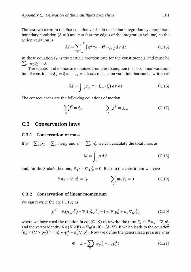
Appendix C. Derivation of the multifluids formalism 161
The last two terms in the first equation vanish in the action integration by appropriateboundary condition (ξ= 0 and τ= 0 at the edges of the integration volume) so theaction variation is
δI =∑
X
∫
gXτX − fX · ξX
dV d t (C.15)
In these equation ΓX is the particle creation rate for the constituent X and must be∑
X mX ΓX = 0.The equations of motion are obtained from the assumption that a common variation
for all constituent ξX = ξ and τX = τ leads to a action variation that can be written as
δI =∫
gextτ− fext · ξ
dV d t (C.16)
The consequences are the following equations of motion:∑
X
fX = fext
∑
X
gX = gext (C.17)
C.3 Conservation laws
C.3.1 Conservation of mass
If ρ =∑
X ρX =∑
X mX nX and ρi =∑
X niX we can calculate the total mass as
M =
∫
Vρ dV (C.18)
and, for the Stoke’s theorem, ∂tρ +∇iρiX = 0. Back to the constituent we have
∂t nX +∇iniX = ΓX
∑
X
mX ΓX = 0 (C.19)
C.3.2 Conservation of linear momentum
We can rewrite the eq. (C.13) as
f Xi = ∂t(nX pX
i ) +∇ j(njX pX
i )− (nX∇i pX0 + n j
X∇i pXj ) (C.20)
where we have used the relation in eq. (C.19) to rewrite the term ΓX as ∂t nX +∇iniX
and the vector identity A× (∇×B) =∇B(A ·B)− (A ·∇) ·B which leads to the equation(nX × (∇× pX ))i = n j
X∇i pXj − n j
X∇ j pXi . Now we define the generalized pressure Ψ as
Ψ = L−∑
X
(nX pX0 + ni
X pXi ) (C.21)

Appendix C. Derivation of the multifluids formalism 162
It’s easy to find, starting from the definition in eq. (C.3), that
dΨ = −∑
X
(nX dp0 + niX dpX
i ) (C.22)
If we calculate the sum of the eq. (C.20) for all the constituents we have the followingrelation
f iext =
∑
X
f ix = ∂tπ
i +∇ j(∑
X
n jX pX
i )−∇iΨ (C.23)
where we use the notation πi to indicate the linear momentum density, ie
πi =∑
X
piXi =
∑
X
nX pXi . (C.24)
As result we can write the conservation law for linear momentum
f iext = ∂tπi +∇ j T
ji (C.25)
T ji =
∑
X
(n jX pX
i ) +Ψδji (C.26)
The energy conservation law can be obtained in a similar way, starting from theeq. (C.14):
gX = niX∂t p
Xi − ni
X∇i pX0 − (∂t nX +∇in
i)pX0 (C.27)
= ∂t(niX pX
i )−∇i(niX pX
0 )− (pX0 ∂t nX + pX
i ∂t niX ) (C.28)
= ∂t(niX pX
i )−∇i(niX pX
0 )− ∂tL (C.29)
The result is that we can write the following equation that express the energy conser-vation law:
gext =∑
X
g x = ∂tH+∇iQi (C.30)
where Qi = −pX0 ni
X and H represent the hamiltonian of the system
H =∑
X
niX pX
i −L (C.31)
C.4 Application to neutron stars
In order to describe a neutron star core, we want to find the class of lagrangian densityL which describe Newtonian hydrodynamics. We postulate that
L(nX , niX ) =
∑
X
mXgi jn
iX n j
X
2nX− E (C.32)

Appendix C. Derivation of the multifluids formalism 163
where gi j is the metric tensor (flat in our case, gi j = δi j), and E is the internal energyof the system. This implies that
−pX0 =
12
mX gi j viX v j
X +∂ E∂ nX
(C.33)
pXi = mX gi j v
jX −
∂ E∂ ni
X
(C.34)
If we want our description to be invariant under a Galileian boost, the term E must bein the following form, as shown in (Prix, 2004):
E(nX , niX ) = E(nX ,∆i
X Y ) (C.35)
where ∆iX Y is the relative velocity between the fluids, i.e.
∆iX Y = v i
X − v iY =
niX
nX−
niY
nY(C.36)
The requirement of isotropy constrains again the form of E to be
E = E(nX ,∆2X Y ) (C.37)
The total differential of the energy function will be
dE =∑
X
µX dnX +12
∑
X ,Y
αX Y d∆2X Y (C.38)
This means that the linear momentum and energy density of the components arecoupled by the term αX Y which encodes the entrainment effect.
pXi = mX gi j v
jX −
∑
Y
2αX Y
nX∆X Y (C.39)
−pX0 = µ
X −mXv2
X
2+ v i
X pXi (C.40)
From the definition of the generalized pressure Ψ, it follows that
E +Ψ =∑
X
nxµX ⇒ dΨ =
∑
X
nX dµX −12
∑
X ,Y
αX Y d∆2X Y (C.41)
It’s easy now, from the relation in eq. (C.23), to write the equation of motion in thisway
f Xi = nX (∂t + v j
x∇ j)pXi + nX∇iµ
X −∑
Y
2αX Y∆jX Y∇i v
Xj (C.42)

Appendix C. Derivation of the multifluids formalism 164
Entropy
Entropy can be included easily in this formulation if we consider it as a constituent ofthe system. The corresponding density is ns = s and its current is ns = svs. Of courseentropy is massless (ms = 0) and we have that µs = T . The internal energy becomes
dE = T ds+∑
X 6=s
µX dnX +12
∑
X ,Y
αX Y d∆2X Y (C.43)
and the momenta are
Θ0 = ps0 = −T − v i
sΘi (C.44)
Θi = psi = −
∑
Y
2αsY
s∆i
sY (C.45)
We can see that, even if entropy has no mass, it has a linear momentum associated dueto the entrainment effect with other fluid constituent. The corresponding equations ofmotion are:
f si = s(∂t + v j
x∇ j)Θi + s∇i T −∑
Y
2αsY∆jsY∇i v
sj (C.46)
gs = v is f s
i + (T + v isΘi)Γs (C.47)

Bibliography
Adams P., Cieplak M., Glaberson W. “Spin-up problem in superfluid 4He”. Phys. Rev. B,32(1):171–177, 1985.DOI: 10.1103/PhysRevB.32.171
Alpar M.A. “Pinning and Threading of Quantized Vortices in the Pulsar Crust Super-fluid”. Astrophys. J., 213:527, 1977.DOI: 10.1086/155183
Alpar M.A., Anderson P.W., Pines D., Shaham J. “Giant glitches and pinned vorticity inthe VELA and other pulsars”. Astrophys. J., 249:L29, 1981.DOI: 10.1086/183652
Alpar M.A., Anderson P.W., Pines D., Shaham J. “Vortex creep and the internal temper-ature of neutron stars. I. General theory”. Astrophys. J., 276, 1984a.
Alpar M.A., Anderson P.W., Pines D., Shaham J. “Vortex creep and the internal temper-ature of neutron stars. II. Vela pulsar”. Astrophys. J., 278, 1984b.
Alpar M.A., Chau H.F., Cheng K.S., Pines D. “Postglitch relaxation of the Crab pulsar:Evidence for crust cracking”. Astrophys. J., 427:L29, 1994.DOI: 10.1086/187357
Alpar M.A., Chau H.F., Cheng K.S., Pines D. “Postglitch Relaxation of the Crab Pulsarafter Its First Four Major Glitches: The Combined Effects of Crust Cracking, Forma-tion of Vortex Depletion Region and Vortex Creep”. Astrophys. J., 459:706, 1996.DOI: 10.1086/176935
Alpar M.A., Langer S.A., Sauls J.A. “Rapid postglitch spin-up of the superfluid core inpulsars”. Astrophys. J., 282:533, 1984c.DOI: 10.1086/162232
165
Bibliography 166
Anderson P.W., Alpar M.A., Pines D., Shaham J. “The rheology of neutron stars.Vortex-line pinning in the crust superfluid”. Philos. Mag. A, 45(2):227–238, 1982.
Anderson P.W., Itoh N. “Pulsar glitches and restlessness as a hard superfluidity phe-nomenon”. Nature, 256(5512):25–27, 1975.DOI: 10.1038/256025a0
Andersson N., Comer G.L. “A flux-conservative formalism for convective and dissipativemulti-fluid systems, with application to Newtonian superfluid neutron stars”. Class.Quantum Gravity, 23(18):5505–5529, 2006.DOI: 10.1088/0264-9381/23/18/003
Andersson N., Glampedakis K., Ho W.C.G., Espinoza C.M. “Pulsar Glitches: The Crustis not Enough”. Phys. Rev. Lett., 109(24):241103, 2012.DOI: 10.1103/PhysRevLett.109.241103
Andersson N., Sidery T., Comer G.L. “Mutual friction in superfluid neutron stars”. Mon.Not. R. Astron. Soc., 368(1):162–170, 2006.DOI: 10.1111/j.1365-2966.2006.10147.x
Andersson N., Sidery T., Comer G.L. “Superfluid neutron star turbulence”. Mon. Not.R. Astron. Soc., 381(2):747–756, 2007.DOI: 10.1111/j.1365-2966.2007.12251.x
Antonelli M. Automaton for spin evolution of isolated pulsar. Master thesis, Universitàdegli studi di Milano, 2014.
Avogadro P., Barranco F., Broglia R., Vigezzi E. “Quantum calculation of vortices in theinner crust of neutron stars”. Phys. Rev. C, 75(1), 2007.DOI: 10.1103/PhysRevC.75.012805
Babaev E. “Unconventional Rotational Responses of Hadronic Superfluids in a NeutronStar Caused by Strong Entrainment and a Σ− Hyperon Gap”. Phys. Rev. Lett.,103(23):231101, 2009.DOI: 10.1103/PhysRevLett.103.231101
Baym G., Pethick C.J., Pines D., Ruderman M. “Spin Up in Neutron Stars : The Futureof the Vela Pulsar”. Nature, 224(5222):872–874, 1969.DOI: 10.1038/224872a0
Bildsten L. “Gravitational Radiation and Rotation of Accreting Neutron Stars”. Astro-phys. J., 501(1):L89–L93, 1998.DOI: 10.1086/311440
Carter B., Chamel N., Haensel P. “Entrainment coefficient and effective mass forconduction neutrons in neutron star crust: macroscopic treatment”. Int. J. Mod.Phys. D, 15(05):777–803, 2006.DOI: 10.1142/S0218271806008504

Bibliography 167
Chamel N. “Effective mass of free neutrons in neutron star crust”. Nucl. Phys. A,773(3-4):263–278, 2006.DOI: 10.1016/j.nuclphysa.2006.04.010
Chamel N. “Two-fluid models of superfluid neutron star cores”. Mon. Not. R. Astron.Soc., 388(2):737–752, 2008.DOI: 10.1111/j.1365-2966.2008.13426.x
Chamel N. “Neutron conduction in the inner crust of a neutron star in the frameworkof the band theory of solids”. Phys. Rev. C, 85(3):035801, 2012.DOI: 10.1103/PhysRevC.85.035801
Chamel N. “Crustal Entrainment and Pulsar Glitches”. Phys. Rev. Lett., 110(1):011101,2013.DOI: 10.1103/PhysRevLett.110.011101
Chamel N., Carter B. “Effect of entrainment on stress and pulsar glitches in stratifiedneutron star crust”. Mon. Not. R. Astron. Soc., 368(2):796–808, 2006.DOI: 10.1111/j.1365-2966.2006.10170.x
Chamel N., Haensel P. “Physics of Neutron Star Crusts”. Living Rev. Relativ., 11, 2008.DOI: 10.12942/lrr-2008-10
Chau H.F., Cheng K.S., Ding K.Y. “Implications of 3P2 superfluidity in the interior ofneutron stars”. Astrophys. J., 399:213, 1992.DOI: 10.1086/171917
Crawford F., Demianski M. “A Comparison of Measured Crab and Vela Glitch HealingParameters with Predictions of Neutron Star Models”. Astrophys. J., 595(2):1052–1057, 2003.DOI: 10.1086/377470
Demorest P.B., Pennucci T., Ransom S.M., Roberts M.S.E., Hessels J.W.T. “A two-solar-mass neutron star measured using Shapiro delay.” Nature, 467(7319):1081–3, 2010.DOI: 10.1038/nature09466
Dodson R.G., Lewis D., McCulloch P. “Two decades of pulsar timing of Vela”. Astrophys.Space Sci., 308(1-4):585–589, 2007.DOI: 10.1007/s10509-007-9372-4
Dodson R.G., McCulloch P.M., Lewis D.R. “High Time Resolution Observations of theJanuary 2000 Glitch in the Vela Pulsar”. Astrophys. J., 564(2):L85–L88, 2002.DOI: 10.1086/339068
Donati P., Pizzochero P.M. “Is there Nuclear Pinning of Vortices in Superfluid Pulsars?”Phys. Rev. Lett., 90(21):4–7, 2003.DOI: 10.1103/PhysRevLett.90.211101

Bibliography 168
Donati P., Pizzochero P.M. “Fully consistent semi-classical treatment of vortex–nucleusinteraction in rotating neutron stars”. Nucl. Phys. A, 742(3-4):363–379, 2004.DOI: 10.1016/j.nuclphysa.2004.07.002
Donati P., Pizzochero P.M. “Realistic energies for vortex pinning in intermediate-densityneutron star matter”. Phys. Lett. B, 640(3):74–81, 2006.DOI: 10.1016/j.physletb.2006.07.047
Douchin F., Haensel P. “A unified equation of state of dense matter and neutron starstructure”. Astron. Astrophys., 380:151–167, 2001.DOI: 10.1051/0004-6361
Elshamouty K.G., Heinke C.O., Sivakoff G.R., Ho W.C.G., Shternin P.S., Yakovlev D.G.,Patnaude D.J., David L. “Measuring the cooling of the neutron star in Cassiopeia Awith all Chandra X-ray observatory detectors”. Astrophys. J., 777(1):22, 2013.DOI: 10.1088/0004-637X/777/1/22
Epstein R.I., Baym G. “Vortex pinning in neutron stars”. Astrophys. J., 328:680, 1988.DOI: 10.1086/166325
Epstein R.I., Baym G. “Vortex drag and the spin-up time scale for pulsar glitches”.Astrophys. J., 387:276, 1992.DOI: 10.1086/171079
Espinoza C.M., Lyne a.G., Stappers B.W., Kramer M. “A study of 315 glitches in therotation of 102 pulsars”. Mon. Not. R. Astron. Soc., 414(2):1679–1704, 2011.DOI: 10.1111/j.1365-2966.2011.18503.x
Fetter A. “Core Structure of a Quantized Vortex”. Phys. Rev. Lett., 27(15):986–988,1971.DOI: 10.1103/PhysRevLett.27.986
Flanagan C. “Twelve years of Glitches in the VELA Pulsar”. Pulsars Probl. progress.Astron. Soc. Pacific Conf. Ser., 105, 1996.
Gandolfi S., Illarionov A., Fantoni S., Pederiva F., Schmidt K. “Equation of State ofSuperfluid Neutron Matter and the Calculation of the 1S0 Pairing Gap”. Phys. Rev.Lett., 101(13):132501, 2008.DOI: 10.1103/PhysRevLett.101.132501
Gandolfi S., Illarionov A.Y., Schmidt K.E., Fantoni S. “Equation of state of low-densityneutron matter, and the 1S0 pairing gap”. Phys. Rev. C, 80(4):045802, 2009.DOI: 10.1103/PhysRevC.80.045802
Glampedakis K., Andersson N. “Hydrodynamical Trigger Mechanism for PulsarGlitches”. Phys. Rev. Lett., 102(14):5, 2009.DOI: 10.1103/PhysRevLett.102.141101

Bibliography 169
Glampedakis K., Andersson N. “Magneto-rotational neutron star evolution: the role ofcore vortex pinning”. Astrophys. J., 740(2):L35, 2011.DOI: 10.1088/2041-8205/740/2/L35
Glendenning N., Moszkowski S. “Reconciliation of neutron-star masses and binding ofthe Λ in hypernuclei”. Phys. Rev. Lett., 67(18):2414–2417, 1991.DOI: 10.1103/PhysRevLett.67.2414
Grill F. Proprietà della materia superfluida in presenza del reticolo nucleare nella crostainterna delle stelle di neutroni. Phd master thesis, Università degli studi di Milano,2011.
Grill F., Pizzochero P.M. “Vortex-lattice interaction in Pulsar Glitches”. J. Phys. Conf.Ser., 342:012004, 2012.DOI: 10.1088/1742-6596/342/1/012004
Gudmundsson E.H., Pethick C.J., Epstein R.I. “Structure of neutron star envelopes”.Astrophys. J., 272:286, 1983.DOI: 10.1086/161292
Gügercinoglu E., Alpar M.A. “Vortex creep against toroidal flux lines, crustal entrain-ment, and pulsar glitches”. Astrophys. J., 788(1):L11, 2014.DOI: 10.1088/2041-8205/788/1/L11
Haensel P., Potekhin A.Y. “Analytical representations of unified equations of state ofneutron-star matter”. Astron. Astrophys., 197:191–197, 2004.DOI: 10.1051/0004-6361
Harvey J., Ruderman M., Shaham J. “Effects of neutron-star superconductivity onmagnetic monopoles and core field decay”. Phys. Rev. D, 33(8):2084–2091, 1986.DOI: 10.1103/PhysRevD.33.2084
Haskell B., Andersson N., Comer G.L. “Dynamics of dissipative multifluid neutron starcores”. Phys. Rev. D, 86(6):063002, 2012a.DOI: 10.1103/PhysRevD.86.063002
Haskell B., Antonopoulou D. “Glitch recoveries in radio-pulsars and magnetars”. Mon.Not. R. Astron. Soc. Lett., 438(1):L16–L20, 2013.DOI: 10.1093/mnrasl/slt146
Haskell B., Degenaar N., Ho W.C.G. “Constraining the physics of the r-mode instabilityin neutron stars with X-ray and ultraviolet observations”. Mon. Not. R. Astron. Soc.,424(1):93–103, 2012b.DOI: 10.1111/j.1365-2966.2012.21171.x

Bibliography 170
Haskell B., Pizzochero P.M., Sidery T. “Modelling pulsar glitches with realistic pinningforces: a hydrodynamical approach”. Mon. Not. R. Astron. Soc., 420:658–671,2012c.DOI: 10.1111/j.1365-2966.2011.20080.x
Haskell B., Samuelsson L., Glampedakis K., Andersson N. “Modelling magneticallydeformed neutron stars”. Mon. Not. R. Astron. Soc., 385(1):531–542, 2008.DOI: 10.1111/j.1365-2966.2008.12861.x
Helfand D.J., Gotthelf E.V., Halpern J.P. “The Vela Pulsar and its Synchrotron Nebula”.Astrophys. J., 556(380):16, 2001.DOI: 10.1086/321533
Ho W.C.G., Andersson N., Haskell B. “Revealing the Physics of r Modes in Low-MassX-Ray Binaries”. Phys. Rev. Lett., 107(10):101101, 2011.DOI: 10.1103/PhysRevLett.107.101101
Jones P.B. “Rotation of the neutron-drip superfluid in pulsars: period discontinuitiesand internal temperatures”. Mon. Not. R. Astron. Soc., 246:315–323, 1990a.
Jones P.B. “Rotation of the neutron-drip superfluid in pulsars: the resistive force”. Mon.Not. R. Astron. Soc., 243:257–262, 1990b.
Jones P.B. “Neutron superfluid spin-down and magnetic field decay in pulsars”. Mon.Not. R. Astron. Soc., 253:279–286, 1991a.DOI: 1991MNRAS.253..279J
Jones P.B. “Rotation of the neutron-drip superfluid in pulsars - The interaction andpinning of vortices”. Astrophys. J., 373:208, 1991b.DOI: 10.1086/170038
Jones P.B. “Rotation of the neutron-drip superfluid in pulsars: the Kelvin phononcontribution to dissipation”. Mon. Not. R. Astron. Soc., 257:501–506, 1992.
Jones P.B. “Type I and two-gap superconductivity in neutron star magnetism”. Mon.Not. R. Astron. Soc., 371(3):1327–1333, 2006.DOI: 10.1111/j.1365-2966.2006.10754.x
Kobyakov D., Pethick C.J. “Towards a Metallurgy of Neutron Star Crusts”. Phys. Rev.Lett., 112(11):112504, 2014.DOI: 10.1103/PhysRevLett.112.112504
Lander S.K., Andersson N., Glampedakis K. “Magnetic neutron star equilibria withstratification and type II superconductivity”. Mon. Not. R. Astron. Soc., 419(1):732–747, 2012.DOI: 10.1111/j.1365-2966.2011.19720.x

Bibliography 171
Larson M.B., Link B. “Simulations of glitches in isolated pulsars”. Mon. Not. R. Astron.Soc., 333(3):613–622, 2002.DOI: 10.1046/j.1365-8711.2002.05439.x
Link B. “Constraining Hadronic Superfluidity with Neutron Star Precession”. Phys. Rev.Lett., 91(10):10–13, 2003.DOI: 10.1103/PhysRevLett.91.101101
Link B. “Dynamics of Quantum Vorticity in a Random Potential”. Phys. Rev. Lett.,102(13):131101, 2009.DOI: 10.1103/PhysRevLett.102.131101
Link B. “Instability of superfluid flow in the neutron star core”. Mon. Not. R. Astron.Soc., 421(3):2682–2691, 2012a.DOI: 10.1111/j.1365-2966.2012.20498.x
Link B. “Instability of superfluid flow in the neutron star inner crust”. Mon. Not. R.Astron. Soc., 422(2):1640–1647, 2012b.DOI: 10.1111/j.1365-2966.2012.20740.x
Link B.K., Epstein R.I. “Mechanics and energetics of vortex unpinning in neutron stars”.Astrophys. J., 373:592, 1991.DOI: 10.1086/170078
Lombardo U., Schulze H.J. Physics of Neutron Star Interiors, volume 578 of LectureNotes in Physics. Springer Berlin Heidelberg, Berlin, Heidelberg, 2001.DOI: 10.1007/3-540-44578-1
Lorenz C., Ravenhall D., Pethick C. “Neutron star crusts”. Phys. Rev. Lett., 70(4):379–382, 1993.DOI: 10.1103/PhysRevLett.70.379
Lyne a.G., Shemar S.L., Graham Smith F. “Statistical studies of pulsar glitches”. Mon.Not. R. Astron. Soc., 315(3):534–542, 2000.DOI: 10.1046/j.1365-8711.2000.03415.x
Manchester R.N., Hobbs G.B., Teoh A., Hobbs M. “The Australia Telescope NationalFacility Pulsar Catalogue”. Astrophys. J., 129:1993–2006, 2005.DOI: 10.1086/428488
Melatos A., Peralta C. “Superfluid Turbulence and Pulsar Glitch Statistics”. Astrophys.J., 662(2):L99–L102, 2007.DOI: 10.1086/518598
Melatos A., Peralta C., Wyithe J.S.B. “Avalanche Dynamics of Radio Pulsar Glitches”.2008.DOI: 10.1086/523349

Bibliography 172
Melatos a., Warszawski L. “Superfluid vortex unpinning as a coherent noise process,and the scale invariance of pulsar glitches”. Astrophys. J., 700(2):1524–1540, 2009.DOI: 10.1088/0004-637X/700/2/1524
Mendell G. “Superfluid hydrodynamics in rotating neutron stars. I - Nondissipativeequations. II - Dissipative effects”. Astrophys. J., 380:515, 1991.DOI: 10.1086/170609
Middleditch J., Marshall F.E., Wang Q.D., Gotthelf E.V., Zhang W. “Predicting theStarquakes in PSR J0537-6910”. Astrophys. J., 652(2):1531–1546, 2006.DOI: 10.1086/508736
Migdal A. “Superfluidity and the moments of inertia of nuclei”. Nucl. Phys., 13(5):655–674, 1959.DOI: 10.1016/0029-5582(59)90264-0
Negele J., Vautherin D. “Neutron star matter at sub-nuclear densities”. Nucl. Phys. A,207(2):298–320, 1973.DOI: 10.1016/0375-9474(73)90349-7
Page D., Prakash M., Lattimer J.M., Steiner A.W. “Rapid Cooling of the Neutron Star inCassiopeia A Triggered by Neutron Superfluidity in Dense Matter”. Phys. Rev. Lett.,106(8):081101, 2011.DOI: 10.1103/PhysRevLett.106.081101
Peralta C., Melatos A. “An unstable superfluid stewartson layer in a differentiallyrotating neutron star”. Astrophys. J., 701(2):L75–L78, 2009.DOI: 10.1088/0004-637X/701/2/L75
Peralta C., Melatos A., Giacobello M., Ooi A. “Global Three-dimensional Flow of a Neu-tron Superfluid in a Spherical Shell in a Neutron Star”. Astrophys. J., 635(2):1224–1232, 2005.DOI: 10.1086/497899
Peralta C., Melatos A., Giacobello M., Ooi A. “Transitions between Turbulent andLaminar Superfluid Vorticity States in the Outer Core of a Neutron Star”. Astrophys.J., 651(2):1079–1091, 2006.DOI: 10.1086/507576
Piekarewicz J., Fattoyev F.J., Horowitz C.J. “Pulsar Glitches: The Crust may be Enough”,2014. eprint: arXiv:1404.2660 .
Pines D., Shaham J., Alpar M.A., Anderson P.W. “Pinned Vorticity in Rotating Superflu-ids, with Application to Neutron Stars”. Suppl. Prog. Theor. Phys., 69, 1980.

Bibliography 173
Pizzochero P.M. “Angular Momentum Transfer in Vela-Like Pulsar Glitches”. Astrophys.J., 743(1):L20, 2011.DOI: 10.1088/2041-8205/743/1/L20
Prix R. “Variational description of multifluid hydrodynamics: Uncharged fluids”. Phys.Rev. D, 69(4), 2004.DOI: 10.1103/PhysRevD.69.043001
Ruderman M. “Neutron Starquakes and Pulsar Periods”. Nature, 223(5206):597–598,1969.DOI: 10.1038/223597b0
Ruderman M. “Crust-breaking by neutron superfluids and the VELA pulsar glitches”.Astrophys. J., 203:213, 1976.DOI: 10.1086/154069
Ruderman M., Zhu T., Chen K. “Neutron Star Magnetic Field Evolution, Crust Move-ment, and Glitches”. Astrophys. J., 492(1):267–280, 1998.DOI: 10.1086/305026
Ruderman M.A., Sutherland P.G. “Rotating Superfluid in Neutron Stars”. Astrophys. J.,190:137, 1974.DOI: 10.1086/152857
Sedrakian A. “Type-I superconductivity and neutron star precession”. Phys. Rev. D,71(8):8–13, 2005.DOI: 10.1103/PhysRevD.71.083003
Sedrakian a., Cordes J.M. “Vortex-interface interactions and generation of glitches inpulsars”. Mon. Not. R. Astron. Soc., 307(2):365–375, 1999.DOI: 10.1046/j.1365-8711.1999.02638.x
Shternin P.S., Yakovlev D.G., Heinke C.O., Ho W.C.G., Patnaude D.J. “Cooling neutronstar in the Cassiopeia A supernova remnant: evidence for superfluidity in the core”.Mon. Not. R. Astron. Soc. Lett., 412(1):L108–L112, 2011.DOI: 10.1111/j.1745-3933.2011.01015.x
Sidery T., Alpar M.A. “The effect of quantized magnetic flux lines on the dynamics ofsuperfluid neutron star cores”. Mon. Not. R. Astron. Soc., 400(4):1859–1867, 2009.DOI: 10.1111/j.1365-2966.2009.15575.x
Sidery T., Passamonti A., Andersson N. “The dynamics of pulsar glitches: contrastingphenomenology with numerical evolutions”. Mon. Not. R. Astron. Soc., 1074:1061–1074, 2010.DOI: 10.1111/j.1365-2966.2010.16497.x

Bibliography 174
Steiner A.W., Gandolfi S., Fattoyev F.J., Newton W.G. “Using Neutron Star Observationsto Determine Crust Thicknesses, Moments of Inertia, and Tidal Deformabilities”,2014. eprint: arXiv:1403.7546 .
Thompson C., Duncan R.C. “The soft gamma repeaters as very strongly magnetizedneutron stars - I. Radiative mechanism for outbursts”. Mon. Not. R. Astron. Soc.,275:255–300, 1995.DOI: 10.1093/mnras/275.2.255
Van Eysden C.A., Melatos A. “Pulsar glitch recovery and the superfluidity coefficientsof bulk nuclear matter”. Mon. Not. R. Astron. Soc., 409(3):1253–1268, 2010.DOI: 10.1111/j.1365-2966.2010.17387.x
Warszawski L., Melatos A. “A cellular automaton model of pulsar glitches”. Mon. Not.R. Astron. Soc., 390(1):175–191, 2008.DOI: 10.1111/j.1365-2966.2008.13662.x
Warszawski L., Melatos A. “Gross-Pitaevskii model of pulsar glitches”. Mon. Not. R.Astron. Soc., 415(2):1611–1630, 2011.DOI: 10.1111/j.1365-2966.2011.18803.x
Warszawski L., Melatos A. “Gravitational-wave bursts and stochastic background fromsuperfluid vortex avalanches during pulsar glitches”. Mon. Not. R. Astron. Soc.,423(3):2058–2074, 2012a.DOI: 10.1111/j.1365-2966.2012.20977.x
Warszawski L., Melatos A. “Knock-on processes in superfluid vortex avalanches andpulsar glitch statistics”. Mon. Not. R. Astron. Soc., 428(3):1911–1926, 2012b.DOI: 10.1093/mnras/sts108
Zhou X.R., Schulze H.J., Zhao E.G., Pan F., Draayer J. “Pairing gaps in neutron stars”.Phys. Rev. C, 70(4):2–5, 2004.DOI: 10.1103/PhysRevC.70.048802
Zuo W., Li Z.H., Lu G.C., Li J.Q., Scheid W., Lombardo U., Schulze H.J., Shen C.W.“1S0 proton and neutron superfluidity in β -stable neutron star matter”. Phys. Lett. B,595(1-4):44–49, 2004.DOI: 10.1016/j.physletb.2004.05.061

List of Publications
As of December 2014
Refereed publications
• “The effect of realistic equations of state and general relativity on the ‘snow-plough’ model for pulsar glitches”.Seveso S., Pizzochero P.M., Haskell B., Mon. Not. R. Astron. Soc., 427(2):1089–1101, 201210.1111/j.1365-2966.2012.21906.x
(Chapter 5)
• “Investigating superconductivity in neutron star interiors with glitch models”Haskell B., Pizzochero P.M., Seveso S., Astrophys. J. L., 764(2):L25, 201310.1088/2041-8205/764/2/L25
(Chapter 6)
Publications under review
• “Mesoscopic pinning forces in neutron star crusts”Seveso S., Pizzochero P.M., Grill F., Haskell B., submitted to Mon. Not. R. Astron.Soc.eprint: arXiv:1408.4298
(Chapter 3)
Publications in preparation
• “Mesoscopic pinning forces in neutron star cores”Seveso S., Pizzochero P.M., Haskell B., to be submitted to Mon. Not. R. Astron.Soc.(Chapter 4)
175

Acknowledgments
This work has been done during the Ph.D. program of “Università degli studi diMilano”, and was partially supported by INFN (Italy) and CompStar, a ResearchNetwork Programme of the European Science Foundation.
I would like to express my special thanks to my supervisor Prof. Pierre Pizzochero, forhis patience, confidence and the help he has gave me: I’m very grateful that you havegiven me the opportunity of growing as a researcher. All the ideas in this thesis comefrom our meetings which have always been very fruitful moments, so again thank you.I would also like to thank Brynmor Haskell for his comments, suggestions and for hisbrilliant advises that have been fundamental for my research.
Questi quattro anni di dottorato sono stati intensi, divertenti e molto soddisfacenti; avolte anche un po’ faticosi. Daniela però mi è sempre stata vicina con infinita pazienzamentre la nostra famiglia si è allargata due volte: grazie per aver tenuto duro e peraccompagnarmi sempre. Anche Michela è stata molto paziente: questa tesi ha rubatoun po’ del “nostro” tempo e so bene di essere in debito.. sono felicissimo adesso dipoterla ripagare recuperando dei bei momenti per crescere insieme.Grazie anche ai miei genitori per il sostegno, a mia sorella Elisa per il lavoro dicorrezione e a tutti quelli che hanno mostrato interesse per questa ricerca e mi sonostati vicini, è stato un aiuto prezioso.E infine Eleonora... questa tesi è per te. Chissà se la leggerai mai quando sarai grande.Probabilmente no, ma non è questo il punto... qui ci puoi trovare solo qualche piccolacosa sulle stelle di neutroni, ma l’universo è enorme, ed è tutto lì per te. Buon viaggio!
Grazie. Stefano
176

Advances in models of Pulsar GlitchesStefano L. Seveso
Physics, Astrophysics and Applied Physics PhD SchoolUniversità degli Studi di Milano
Advances in models of Pulsar Glitches
Neutron stars are surely one of the most interesting astronomical objects: in no other place of the observable universe, in fact, matter is so compressed that the density reaches and overcomes the nuclear saturation value. This is a so extreme condition that in no terrestrial laboratory we can directly re-produce it in order to study its properties. Neutron stars are therefore a very fascinating research field that can bring us to a deeper understanding of this exotic matter, by modeling the observations of peculiar phenomena rrelated to these stars. This thesis is focused on the pulsar glitches, which are rapid jumps in the rotation velocity of the star.
Shortly after the first glitches were observed it was suggested that they could be due to a superfluid component in the stellar interior that could store angular momentum thanks to the pinning interaction between super-fluid vortexes and crustal lattice. This qualitative idea suggests that the problem must be faced by merging results which come from the micro-physics point of view into a more macroscopic simulation. Therefore the mesoscopic calculation of the pinning force profiles is addressed, both for the crust of a neutron star and for the core. These results are used in static models which can reproduce the physical observable parameters.
The whole time evolution of a glitch can be followed thanks the develop-ment of a dynamical model. The multifluids formalism is implemented in a consistent simulation, which take into account realistic physical inputs like equation of state, entrainment and drag forces: the rise and the recovery of a glitch is analyzed in connection with the relevant parameters of the model. By comparing the results with the observational data, important aspects about this phenomenon and neutron stars in general are dis-cussed here.
Advances in m
odels of Pulsa
r Glitches
Seveso