STATISTICSsite.iugaza.edu.ps/mriffi/files/2018/02/ch11.pdf · Copyright © 2017, 2013, 2010 Pearson...
166
STATISTICS INFORMED DECISIONS USING DATA Fifth Edition Chapter 11 Inferences on Two Samples Copyright © 2017, 2013, 2010 Pearson Education, Inc. All Rights Reserved
Transcript of STATISTICSsite.iugaza.edu.ps/mriffi/files/2018/02/ch11.pdf · Copyright © 2017, 2013, 2010 Pearson...

STATISTICSINFORMED DECISIONS USING DATAFifth Edition
Chapter 11
Inferences on Two Samples
Copyright © 2017, 2013, 2010 Pearson Education, Inc. All Rights Reserved

Copyright © 2017, 2013, 2010 Pearson Education, Inc. All Rights Reserved
11.1 Inference about Two Population ProportionsLearning Objectives
1. Distinguish between independent and dependent sampling
2. Test hypotheses regarding two proportions from independent samples
3. Construct and interpret confidence intervals for the difference between two population proportions
4. Determine the sample size necessary for estimating the difference between two population proportions

Copyright © 2017, 2013, 2010 Pearson Education, Inc. All Rights Reserved
11.1 Inference about Two Population Proportions11.1.1 Distinguish between Independent and Dependent Sampling (1 of 4)
A sampling method is independent when the individuals selected for one sample do not dictate which individuals are to be in a second sample. A sampling method is dependentwhen the individuals selected to be in one sample are used to determine the individuals to be in the second sample.

Copyright © 2017, 2013, 2010 Pearson Education, Inc. All Rights Reserved
11.1 Inference about Two Population Proportions11.1.1 Distinguish between Independent and Dependent Sampling (2 of 4)
Dependent samples are often referred to as matched-pairssamples. It is possible for an individual to be matched against him- or herself.

Copyright © 2017, 2013, 2010 Pearson Education, Inc. All Rights Reserved
11.1 Inference about Two Population Proportions11.1.1 Distinguish between Independent and Dependent Sampling (3 of 4)
Parallel Example 1: Distinguish between Independent and Dependent Sampling
For each of the following, determine whether the sampling method is independent or dependent.
A researcher wants to know whether the price of a one night stay at a Holiday Inn Express is less than the price of a one night stay at a Red Roof Inn. She randomly selects 8 towns where the location of the hotels is close to each other and determines the price of a one night stay.
A researcher wants to know whether the “state” quarters (introduced in 1999) have a mean weight that is different from “traditional” quarters. He randomly selects 18 “state” quarters and 16 “traditional” quarters and compares their weights.

Copyright © 2017, 2013, 2010 Pearson Education, Inc. All Rights Reserved
11.1 Inference about Two Population Proportions11.1.1 Distinguish between Independent and Dependent Sampling (4 of 4)
Solution
The sampling method is dependent since the 8 Holiday Inn Express hotels can be matched with one of the 8 Red Roof Inn hotels by town.
The sampling method is independent since the “state” quarters which were sampled had no bearing on which “traditional”quarters were sampled.

Copyright © 2017, 2013, 2010 Pearson Education, Inc. All Rights Reserved
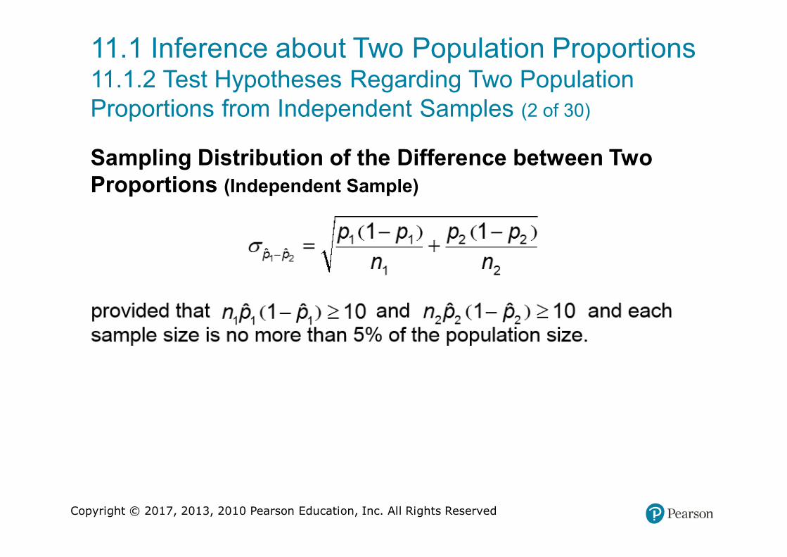
11.1 Inference about Two Population Proportions11.1.2 Test Hypotheses Regarding Two Population Proportions from Independent Samples (1 of 30)
Sampling Distribution of the Difference between Two Proportions (Independent Sample)
Copyright © 2017, 2013, 2010 Pearson Education, Inc. All Rights Reserved
11.1 Inference about Two Population Proportions11.1.2 Test Hypotheses Regarding Two Population Proportions from Independent Samples (2 of 30)
Sampling Distribution of the Difference between Two Proportions (Independent Sample)

Copyright © 2017, 2013, 2010 Pearson Education, Inc. All Rights Reserved
11.1 Inference about Two Population Proportions11.1.2 Test Hypotheses Regarding Two Population Proportions from Independent Samples (3 of 30)
Sampling Distribution of the Difference between Two Proportions
Copyright © 2017, 2013, 2010 Pearson Education, Inc. All Rights Reserved
11.1 Inference about Two Population Proportions11.1.2 Test Hypotheses Regarding Two Population Proportions from Independent Samples (4 of 30)

Copyright © 2017, 2013, 2010 Pearson Education, Inc. All Rights Reserved
11.1 Inference about Two Population Proportions11.1.2 Test Hypotheses Regarding Two Population Proportions from Independent Samples (5 of 30)
Hypothesis Test Regarding the Difference between Two Population Proportions
To test hypotheses regarding two population proportions, p1 and p2, we can use the steps that follow, provided that:
– the samples are independently obtained using simple random sampling,

Copyright © 2017, 2013, 2010 Pearson Education, Inc. All Rights Reserved
11.1 Inference about Two Population Proportions11.1.2 Test Hypotheses Regarding Two Population Proportions from Independent Samples (6 of 30)
Step 1: Determine the null and alternative hypotheses. The hypotheses can be structured in one of three ways:
Two-Tailed Left-Tailed Right-Tailed
H0: p1 = p2 H0: p1 = p2 H0: p1 = p2
H1: p1 ≠ p2 H1: p1 < p2 H1: p1 > p2
Note: p1 is the population proportion for population 1, and p2 is the population proportion for population 2.

Copyright © 2017, 2013, 2010 Pearson Education, Inc. All Rights Reserved
11.1 Inference about Two Population Proportions11.1.2 Test Hypotheses Regarding Two Population Proportions from Independent Samples (7 of 30)
Step 2: Select a level of significance, α, depending on the seriousness of making a Type I error.

Copyright © 2017, 2013, 2010 Pearson Education, Inc. All Rights Reserved
11.1 Inference about Two Population Proportions11.1.2 Test Hypotheses Regarding Two Population Proportions from Independent Samples (8 of 30)
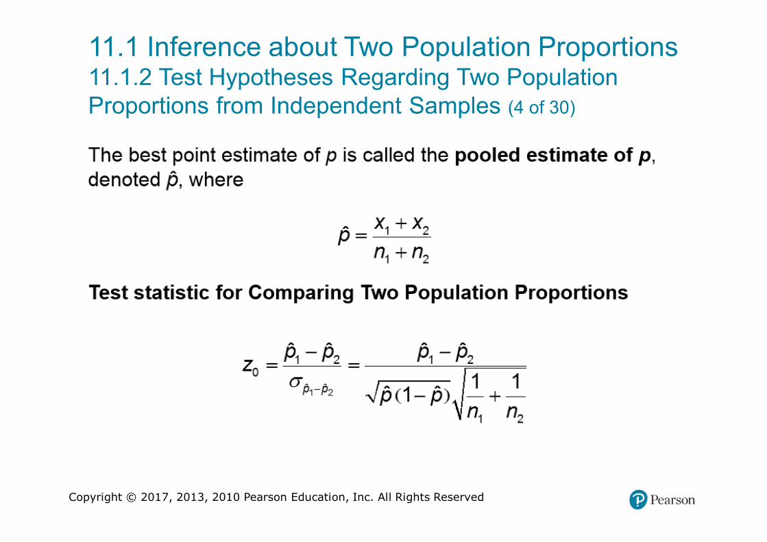
Classical Approach
Step 3: Compute the test statistic

Copyright © 2017, 2013, 2010 Pearson Education, Inc. All Rights Reserved
11.1 Inference about Two Population Proportions11.1.2 Test Hypotheses Regarding Two Population Proportions from Independent Samples (9 of 30)
Classical Approach
Use Table V to determine the critical value.
Copyright © 2017, 2013, 2010 Pearson Education, Inc. All Rights Reserved
11.1 Inference about Two Population Proportions11.1.2 Test Hypotheses Regarding Two Population Proportions from Independent Samples (10 of 30)
Classical Approach
Two-Tailed

Copyright © 2017, 2013, 2010 Pearson Education, Inc. All Rights Reserved
11.1 Inference about Two Population Proportions11.1.2 Test Hypotheses Regarding Two Population Proportions from Independent Samples (11 of 30)
Classical Approach
Left-Tailed

Copyright © 2017, 2013, 2010 Pearson Education, Inc. All Rights Reserved
11.1 Inference about Two Population Proportions11.1.2 Test Hypotheses Regarding Two Population Proportions from Independent Samples (12 of 30)
Classical Approach
Right-Tailed

Copyright © 2017, 2013, 2010 Pearson Education, Inc. All Rights Reserved
11.1 Inference about Two Population Proportions11.1.2 Test Hypotheses Regarding Two Population Proportions from Independent Samples (13 of 30)
P-value Approach
By Hand Step 3: Compute the test statistic

Copyright © 2017, 2013, 2010 Pearson Education, Inc. All Rights Reserved
11.1 Inference about Two Population Proportions11.1.2 Test Hypotheses Regarding Two Population Proportions from Independent Samples (14 of 30)
P-value Approach
Use Table V to determine the P-Value.
Copyright © 2017, 2013, 2010 Pearson Education, Inc. All Rights Reserved
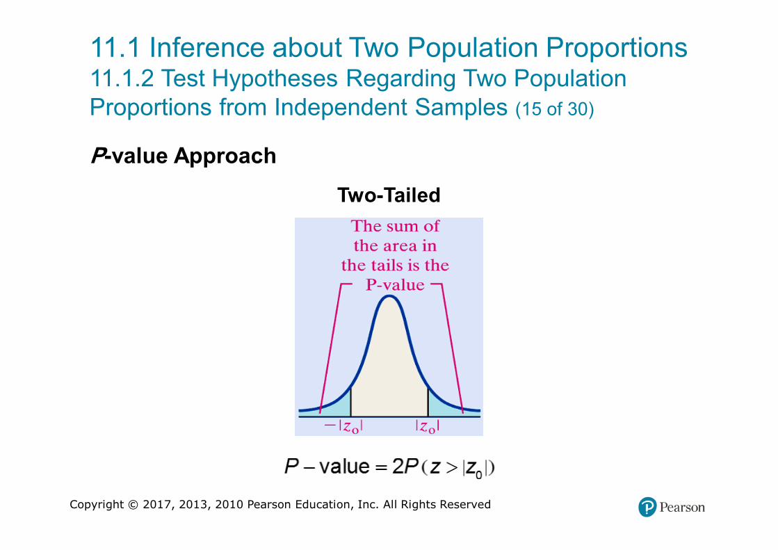
11.1 Inference about Two Population Proportions11.1.2 Test Hypotheses Regarding Two Population Proportions from Independent Samples (15 of 30)
P-value Approach
Two-Tailed

Copyright © 2017, 2013, 2010 Pearson Education, Inc. All Rights Reserved
11.1 Inference about Two Population Proportions11.1.2 Test Hypotheses Regarding Two Population Proportions from Independent Samples (16 of 30)
P-value Approach
Left-Tailed

Copyright © 2017, 2013, 2010 Pearson Education, Inc. All Rights Reserved
11.1 Inference about Two Population Proportions11.1.2 Test Hypotheses Regarding Two Population Proportions from Independent Samples (17 of 30)
P-value Approach
Right-Tailed

Copyright © 2017, 2013, 2010 Pearson Education, Inc. All Rights Reserved
11.1 Inference about Two Population Proportions11.1.2 Test Hypotheses Regarding Two Population Proportions from Independent Samples (18 of 30)
P-value Approach
Technology Step 3: Use a statistical spreadsheet or calculator with statistical capabilities to obtain the P-value. The directions for obtaining the P-value using the TI-83/84 Plus graphing calculator, Excel, MINITAB, and StatCrunch are in the Technology Step-by-Step in the text.

Copyright © 2017, 2013, 2010 Pearson Education, Inc. All Rights Reserved
11.1 Inference about Two Population Proportions11.1.2 Test Hypotheses Regarding Two Population Proportions from Independent Samples (19 of 30)
Classical Approach
Step 4: Compare the critical value with the test statistic:
Copyright © 2017, 2013, 2010 Pearson Education, Inc. All Rights Reserved
11.1 Inference about Two Population Proportions11.1.2 Test Hypotheses Regarding Two Population Proportions from Independent Samples (20 of 30)
P-value Approach
Step 4: If P-value < α, reject the null hypothesis.

Copyright © 2017, 2013, 2010 Pearson Education, Inc. All Rights Reserved
11.1 Inference about Two Population Proportions11.1.2 Test Hypotheses Regarding Two Population Proportions from Independent Samples (21 of 30)
P-value Approach
Step 5: State the conclusion.

Copyright © 2017, 2013, 2010 Pearson Education, Inc. All Rights Reserved
11.1 Inference about Two Population Proportions11.1.2 Test Hypotheses Regarding Two Population Proportions from Independent Samples (22 of 30)
Parallel Example 1: Testing Hypotheses Regarding Two Population Proportions
An economist believes that the percentage of urban households with Internet access is greater than the percentage of rural households with Internet access. He obtains a random sample of 800 urban households and finds that 338 of them have Internet access. He obtains a random sample of 750 rural households and finds that 292 of them have Internet access. Test the economist’s claim at the α = 0.05 level of significance.

Copyright © 2017, 2013, 2010 Pearson Education, Inc. All Rights Reserved
11.1 Inference about Two Population Proportions11.1.2 Test Hypotheses Regarding Two Population Proportions from Independent Samples (23 of 30)
Solution
We must first verify that the requirements are satisfied:
The samples are simple random samples that were obtained independently.

Copyright © 2017, 2013, 2010 Pearson Education, Inc. All Rights Reserved
11.1 Inference about Two Population Proportions11.1.2 Test Hypotheses Regarding Two Population Proportions from Independent Samples (24 of 30)
Solution
Step 1: We want to determine whether the percentage of urban households with Internet access is greater than the percentage of rural households with Internet access. So,
H0: p1 = p2 versus H1: p1 > p2
or, equivalently,
H0: p1 − p2 = 0 versus H1: p1 − p2 > 0
Step 2: The level of significance is α = 0.05.

Copyright © 2017, 2013, 2010 Pearson Education, Inc. All Rights Reserved
11.1 Inference about Two Population Proportions11.1.2 Test Hypotheses Regarding Two Population Proportions from Independent Samples (25 of 30)
Solution

Copyright © 2017, 2013, 2010 Pearson Education, Inc. All Rights Reserved
11.1 Inference about Two Population Proportions11.1.2 Test Hypotheses Regarding Two Population Proportions from Independent Samples (26 of 30)
Solution: Classical Approach
This is a right-tailed test with α = 0.05.The critical value is z0.05 = 1.645.

Copyright © 2017, 2013, 2010 Pearson Education, Inc. All Rights Reserved
11.1 Inference about Two Population Proportions11.1.2 Test Hypotheses Regarding Two Population Proportions from Independent Samples (27 of 30)
Step 4: Since the test statistic, z0 = 1.33 is less than the critical value z.05 = 1.645, we fail to reject the null hypothesis.

Copyright © 2017, 2013, 2010 Pearson Education, Inc. All Rights Reserved
11.1 Inference about Two Population Proportions11.1.2 Test Hypotheses Regarding Two Population Proportions from Independent Samples (28 of 30)
Solution: P-value Approach
Because this is a right-tailed test, the P-value is the area under the normal to the right of the test statistic z0 = 1.33.That is, P-value = P(Z > 1.33) ≈ 0.09.

Copyright © 2017, 2013, 2010 Pearson Education, Inc. All Rights Reserved
11.1 Inference about Two Population Proportions11.1.2 Test Hypotheses Regarding Two Population Proportions from Independent Samples (29 of 30)
Solution: P-value Approach
Step 4: Since the P-value is greater than the level of significance α = 0.05, we fail to reject the null hypothesis.

Copyright © 2017, 2013, 2010 Pearson Education, Inc. All Rights Reserved
11.1 Inference about Two Population Proportions11.1.2 Test Hypotheses Regarding Two Population Proportions from Independent Samples (30 of 30)
Solution
Step 5: There is insufficient evidence at the α = 0.05 level to conclude that the percentage of urban households with Internet access is greater than the percentage of rural households with Internet access.
Copyright © 2017, 2013, 2010 Pearson Education, Inc. All Rights Reserved
11.1 Inference about Two Population Proportions11.1.3 Construct and Interpret Confidence Intervals for the
Difference between Two Population Proportions (1 of 6)
Constructing a (1 − α) • 100% Confidence Interval for the Difference between Two Population Proportions
To construct a (1 − α) • 100% confidence interval for the difference between two population proportions, the following requirements must be satisfied:
1. the samples are obtained independently using simple random sampling,

Copyright © 2017, 2013, 2010 Pearson Education, Inc. All Rights Reserved
11.1 Inference about Two Population Proportions11.1.3 Construct and Interpret Confidence Intervals for the
Difference between Two Population Proportions (2 of 6)
Constructing a (1 − α) • 100% Confidence Interval for the Difference between Two Population Proportions
Provided that these requirements are met, a (1 − α) • 100% confidence interval for p1 − p2 is given by

Copyright © 2017, 2013, 2010 Pearson Education, Inc. All Rights Reserved
11.1 Inference about Two Population Proportions11.1.3 Construct and Interpret Confidence Intervals for the
Difference between Two Population Proportions (3 of 6)
Parallel Example 3: Constructing a Confidence Interval for the Difference between Two Population Proportions
An economist obtains a random sample of 800 urban households and finds that 338 of them have Internet access. He obtains a random sample of 750 rural households and finds that 292 of them have Internet access. Find a 99% confidence interval for the difference between the proportion of urban households that have Internet access and the proportion of rural households that have Internet access.

Copyright © 2017, 2013, 2010 Pearson Education, Inc. All Rights Reserved
11.1 Inference about Two Population Proportions11.1.3 Construct and Interpret Confidence Intervals for the
Difference between Two Population Proportions (4 of 6)
Solution
We have already verified the requirements for constructing a confidence interval for the difference between two population proportions in the previous example.

Copyright © 2017, 2013, 2010 Pearson Education, Inc. All Rights Reserved
11.1 Inference about Two Population Proportions11.1.3 Construct and Interpret Confidence Intervals for the
Difference between Two Population Proportions (5 of 6)
Solution
Thus,

Copyright © 2017, 2013, 2010 Pearson Education, Inc. All Rights Reserved
11.1 Inference about Two Population Proportions11.1.3 Construct and Interpret Confidence Intervals for the
Difference between Two Population Proportions (6 of 6)
Solution
We are 99% confident that the difference between the proportion of urban households that have Internet access and the proportion of rural households that have Internet access is between −0.03 and 0.10. Since the confidence interval contains 0, we are unable to conclude that the proportion of urban households with Internet access is greater than the proportion of rural households with Internet access.

Copyright © 2017, 2013, 2010 Pearson Education, Inc. All Rights Reserved
11.1 Inference about Two Population Proportions11.1.4 Determine the Sample Size Necessary for Estimating the Difference between Two Population Proportions (1 of 4)
Sample Size for Estimating p1 − p2
The sample size required to obtain a (1 − α)•100% confidence interval with a margin of error, E, is given by

Copyright © 2017, 2013, 2010 Pearson Education, Inc. All Rights Reserved
11.1 Inference about Two Population Proportions11.1.4 Determine the Sample Size Necessary for Estimating the Difference between Two Population Proportions (2 of 4)
Parallel Example 5: Determining Sample Size
A doctor wants to estimate the difference in the proportion of 15-19 year old mothers that received prenatal care and the proportion of 30-34 year old mothers that received prenatal care. What sample size should be obtained if she wished the estimate to be within 2 percentage points with 95% confidence assuming:
A. she uses the results of the National Vital Statistics Report results in which 98% of the 15-19 year old mothers received prenatal care and 99.2% of 30-34 year old mothers received prenatal care.
B. she does not use any prior estimates.

Copyright © 2017, 2013, 2010 Pearson Education, Inc. All Rights Reserved
11.1 Inference about Two Population Proportions11.1.4 Determine the Sample Size Necessary for Estimating the Difference between Two Population Proportions (3 of 4)
The doctor must sample 265 randomly selected 15-19 year old mothers and 265 randomly selected 30-34 year old mothers.

Copyright © 2017, 2013, 2010 Pearson Education, Inc. All Rights Reserved
11.1 Inference about Two Population Proportions11.1.4 Determine the Sample Size Necessary for Estimating the Difference between Two Population Proportions (4 of 4)
The doctor must sample 4802 randomly selected 15-19 year old mothers and 4802 randomly selected 30-34 year old mothers. Note that having prior estimates of p1 and p2 reduces the number of mothers that need to be surveyed.
Copyright © 2017, 2013, 2010 Pearson Education, Inc. All Rights Reserved
11.2 Inference about Two Means: Dependent SamplesLearning Objectives
1. Test hypotheses for a population mean from matched-pairs data
2. Construct and interpret confidence intervals about the population mean difference of matched-pairs data

Copyright © 2017, 2013, 2010 Pearson Education, Inc. All Rights Reserved
11.2 Inference about Two Means: Dependent Samples11.2.1 Test Hypotheses for a Population Mean from Matched-Pairs Data (1 of 30)
“In Other Words”
Statistical inference methods on matched-pairs data use the same methods as inference on a single population mean, except that the differences are analyzed.

Copyright © 2017, 2013, 2010 Pearson Education, Inc. All Rights Reserved
11.2 Inference about Two Means: Dependent Samples11.2.1 Test Hypotheses for a Population Mean from Matched-Pairs Data (2 of 30)
Testing Hypotheses Regarding the Difference of Two Means Using a Matched-Pairs Design
To test hypotheses regarding the mean difference of data obtained form a dependent sample (matched-pairs data), use the following steps. provided that
• the sample is obtained using simple random sampling,
• the sample data are matched pairs,
• the differences are normally distributed with no outliers or the sample size, n, is large (n ≥ 30),
• the sampled values are independent
Copyright © 2017, 2013, 2010 Pearson Education, Inc. All Rights Reserved
11.2 Inference about Two Means: Dependent Samples11.2.1 Test Hypotheses for a Population Mean from Matched-Pairs Data (3 of 30)
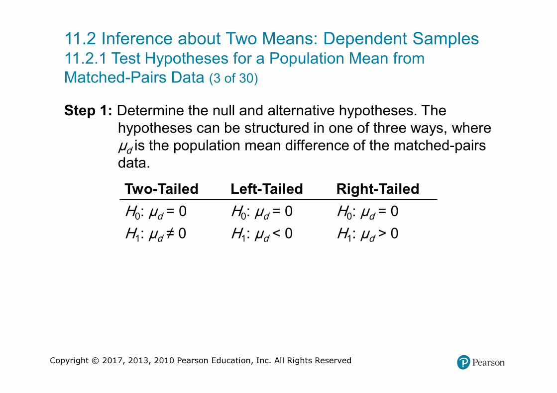
Step 1: Determine the null and alternative hypotheses. The hypotheses can be structured in one of three ways, where μd is the population mean difference of the matched-pairs data.
Two-Tailed Left-Tailed Right-Tailed
H0: µd = 0 H0: µd = 0 H0: µd = 0
H1: µd ≠ 0 H1: µd < 0 H1: µd > 0
Copyright © 2017, 2013, 2010 Pearson Education, Inc. All Rights Reserved
11.2 Inference about Two Means: Dependent Samples11.2.1 Test Hypotheses for a Population Mean from Matched-Pairs Data (4 of 30)
Step 2: Select a level of significance, α, depending on the seriousness of making a Type I error.
Copyright © 2017, 2013, 2010 Pearson Education, Inc. All Rights Reserved
11.2 Inference about Two Means: Dependent Samples11.2.1 Test Hypotheses for a Population Mean from Matched-Pairs Data (5 of 30)
Classical Approach
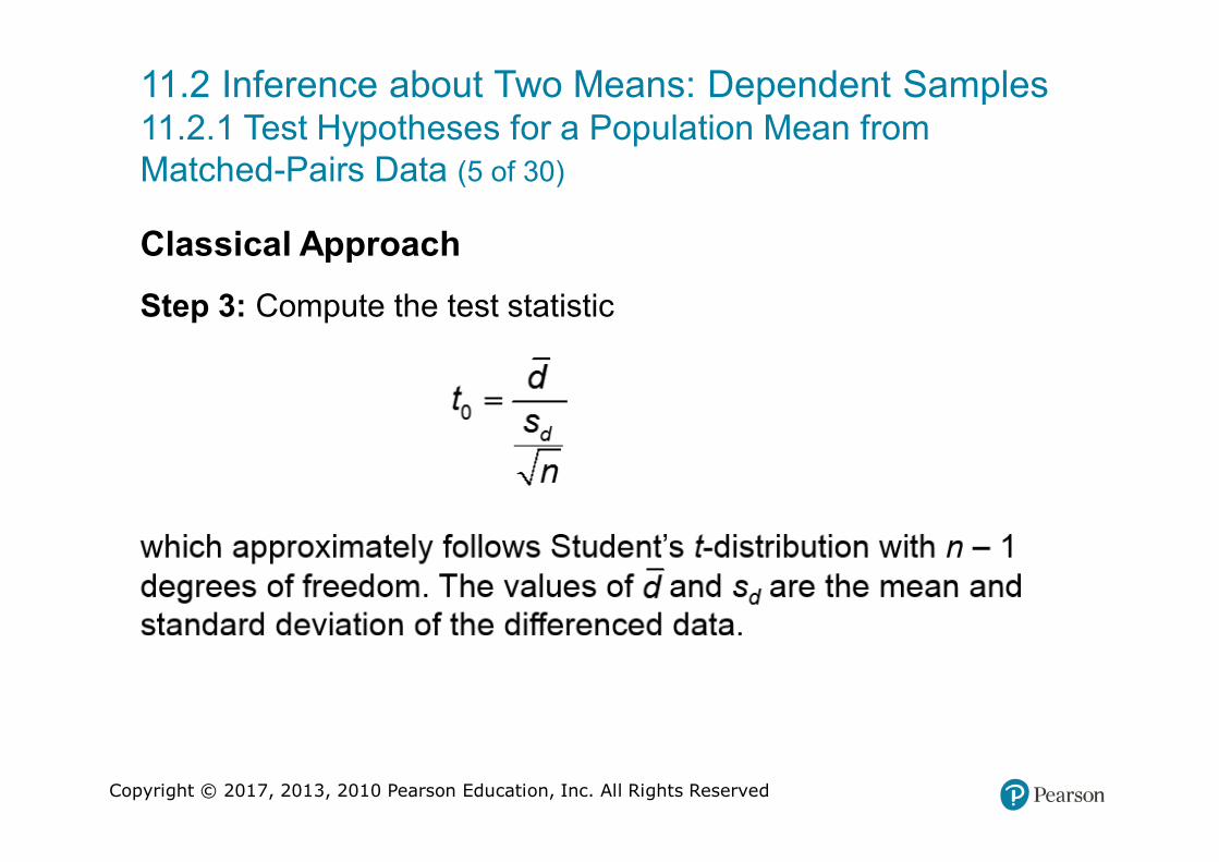
Step 3: Compute the test statistic

Copyright © 2017, 2013, 2010 Pearson Education, Inc. All Rights Reserved
11.2 Inference about Two Means: Dependent Samples11.2.1 Test Hypotheses for a Population Mean from Matched-Pairs Data (6 of 30)
Classical Approach
Use Table VII to determine the critical value using n − 1 degrees of freedom.

Copyright © 2017, 2013, 2010 Pearson Education, Inc. All Rights Reserved
11.2 Inference about Two Means: Dependent Samples11.2.1 Test Hypotheses for a Population Mean from Matched-Pairs Data (7 of 30)
Classical Approach
Two-Tailed

Copyright © 2017, 2013, 2010 Pearson Education, Inc. All Rights Reserved
11.2 Inference about Two Means: Dependent Samples11.2.1 Test Hypotheses for a Population Mean from Matched-Pairs Data (8 of 30)
Classical Approach
Left-Tailed
Copyright © 2017, 2013, 2010 Pearson Education, Inc. All Rights Reserved
11.2 Inference about Two Means: Dependent Samples11.2.1 Test Hypotheses for a Population Mean from Matched-Pairs Data (9 of 30)
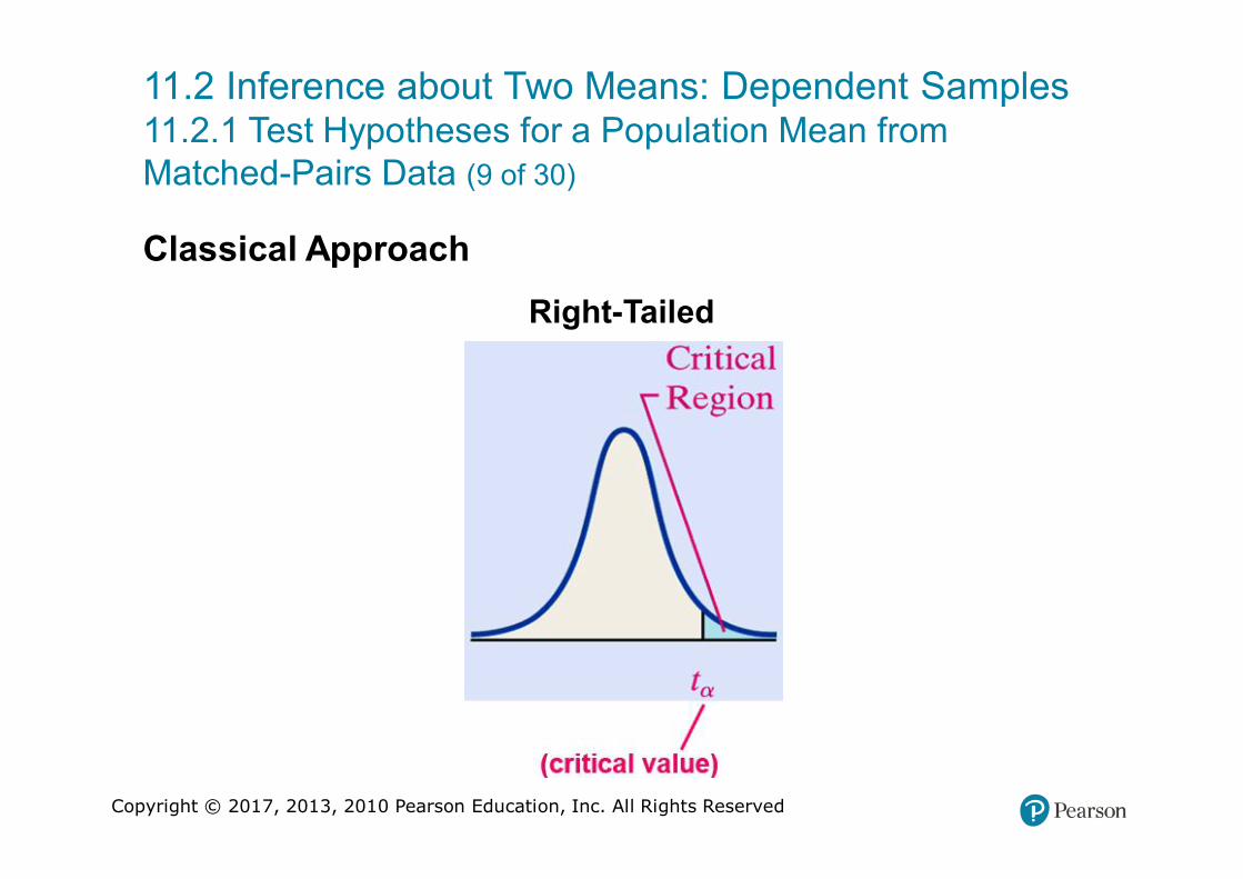
Classical Approach
Right-Tailed

Copyright © 2017, 2013, 2010 Pearson Education, Inc. All Rights Reserved
11.2 Inference about Two Means: Dependent Samples11.2.1 Test Hypotheses for a Population Mean from Matched-Pairs Data (10 of 30)
Classical Approach
Step 4: Compare the critical value with the test statistic:

Copyright © 2017, 2013, 2010 Pearson Education, Inc. All Rights Reserved
11.2 Inference about Two Means: Dependent Samples11.2.1 Test Hypotheses for a Population Mean from Matched-Pairs Data (11 of 30)
P-value Approach
Step 3: Compute the test statistic
Copyright © 2017, 2013, 2010 Pearson Education, Inc. All Rights Reserved
11.2 Inference about Two Means: Dependent Samples11.2.1 Test Hypotheses for a Population Mean from Matched-Pairs Data (12 of 30)
P-value Approach
Use Table VII to approximate the P-value using n − 1 degrees of freedom.

Copyright © 2017, 2013, 2010 Pearson Education, Inc. All Rights Reserved
11.2 Inference about Two Means: Dependent Samples11.2.1 Test Hypotheses for a Population Mean from Matched-Pairs Data (13 of 30)
P-value Approach
Two-Tailed

Copyright © 2017, 2013, 2010 Pearson Education, Inc. All Rights Reserved
11.2 Inference about Two Means: Dependent Samples11.2.1 Test Hypotheses for a Population Mean from Matched-Pairs Data (14 of 30)
P-value Approach
Left-Tailed

Copyright © 2017, 2013, 2010 Pearson Education, Inc. All Rights Reserved
11.2 Inference about Two Means: Dependent Samples11.2.1 Test Hypotheses for a Population Mean from Matched-Pairs Data (15 of 30)
P-value Approach
Right-Tailed

Copyright © 2017, 2013, 2010 Pearson Education, Inc. All Rights Reserved
11.2 Inference about Two Means: Dependent Samples11.2.1 Test Hypotheses for a Population Mean from Matched-Pairs Data (16 of 30)
P-value Approach
Technology Step 3: Use a statistical spreadsheet or calculator with statistical capabilities to obtain the P-value. The directions for obtaining the P-value using the TI-83/84 Plus graphing calculator, MINITAB, Excel and StatCrunch, are in the Technology Step-by-Step in the text.

Copyright © 2017, 2013, 2010 Pearson Education, Inc. All Rights Reserved
11.2 Inference about Two Means: Dependent Samples11.2.1 Test Hypotheses for a Population Mean from Matched-Pairs Data (17 of 30)
P-value Approach
Step 4: If P-value < α, reject the null hypothesis.
Copyright © 2017, 2013, 2010 Pearson Education, Inc. All Rights Reserved
11.2 Inference about Two Means: Dependent Samples11.2.1 Test Hypotheses for a Population Mean from Matched-Pairs Data (18 of 30)
P-value Approach
Step 5: State the conclusion.

Copyright © 2017, 2013, 2010 Pearson Education, Inc. All Rights Reserved
11.2 Inference about Two Means: Dependent Samples11.2.1 Test Hypotheses for a Population Mean from Matched-Pairs Data (19 of 30)
These procedures are robust, which means that minor departures from normality will not adversely affect the results. However, if the data have outliers, the procedure should not be used.

Copyright © 2017, 2013, 2010 Pearson Education, Inc. All Rights Reserved
11.2 Inference about Two Means: Dependent Samples11.2.1 Test Hypotheses for a Population Mean from Matched-Pairs Data (20 of 30)
Parallel Example 2: Testing a Claim Regarding Matched-Pairs Data
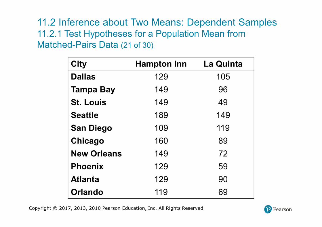
The following data represent the cost of a one night stay in Hampton Inn Hotels and La Quinta Inn Hotels for a random sample of 10 cities. Test the claim that Hampton Inn Hotels are priced differently than La Quinta Hotels at the α = 0.05 level of significance.
Copyright © 2017, 2013, 2010 Pearson Education, Inc. All Rights Reserved
11.2 Inference about Two Means: Dependent Samples11.2.1 Test Hypotheses for a Population Mean from Matched-Pairs Data (21 of 30)
City Hampton Inn La Quinta
Dallas 129 105
Tampa Bay 149 96
St. Louis 149 49
Seattle 189 149
San Diego 109 119
Chicago 160 89
New Orleans 149 72
Phoenix 129 59
Atlanta 129 90
Orlando 119 69

Copyright © 2017, 2013, 2010 Pearson Education, Inc. All Rights Reserved
11.2 Inference about Two Means: Dependent Samples11.2.1 Test Hypotheses for a Population Mean from Matched-Pairs Data (22 of 30)
Solution
This is a matched-pairs design since the hotel prices come from the same ten cities. To test the hypothesis, we first compute the differences and then verify that the differences come from a population that is approximately normally distributed with no outliers because the sample size is small.

Copyright © 2017, 2013, 2010 Pearson Education, Inc. All Rights Reserved
11.2 Inference about Two Means: Dependent Samples11.2.1 Test Hypotheses for a Population Mean from Matched-Pairs Data (23 of 30)
Solution

Copyright © 2017, 2013, 2010 Pearson Education, Inc. All Rights Reserved
11.2 Inference about Two Means: Dependent Samples11.2.1 Test Hypotheses for a Population Mean from Matched-Pairs Data (24 of 30)
Solution

Copyright © 2017, 2013, 2010 Pearson Education, Inc. All Rights Reserved
11.2 Inference about Two Means: Dependent Samples11.2.1 Test Hypotheses for a Population Mean from Matched-Pairs Data (25 of 30)
Solution
Step 1: We want to determine if the prices differ:
H0: μd = 0 versus H1: μd ≠ 0
Step 2: The level of significance is α = 0.05.
Step 3: The test statistic is

Copyright © 2017, 2013, 2010 Pearson Education, Inc. All Rights Reserved
11.2 Inference about Two Means: Dependent Samples11.2.1 Test Hypotheses for a Population Mean from Matched-Pairs Data (26 of 30)
Solution: Classical Approach
This is a two-tailed test so the critical values at the α = 0.05 level of significance with n − 1 = 10 − 1 = 9 degrees of freedom are −t0.025 = −2.262 and t0.025 = 2.262.

Copyright © 2017, 2013, 2010 Pearson Education, Inc. All Rights Reserved
11.2 Inference about Two Means: Dependent Samples11.2.1 Test Hypotheses for a Population Mean from Matched-Pairs Data (27 of 30)
Solution: Classical Approach
Step 4: Since the test statistic, t0 = 5.27 is greater than the critical value t.025 = 2.262, we reject the null hypothesis.

Copyright © 2017, 2013, 2010 Pearson Education, Inc. All Rights Reserved
11.2 Inference about Two Means: Dependent Samples11.2.1 Test Hypotheses for a Population Mean from Matched-Pairs Data (28 of 30)
Solution: P-value Approach
Because this is a two-tailed test, the P-value is two times the area under the t-distribution with n − 1 = 10 − 1 = 9 degrees of freedom to the right of the test statistic t0 = 5.27.
That is, P-value = 2P(t > 5.27) ≈ 2(0.00026) = 0.00052 (using technology). Approximately 5 samples in 10,000 will yield results at least as extreme as we obtained if the null hypothesis is true.

Copyright © 2017, 2013, 2010 Pearson Education, Inc. All Rights Reserved
11.2 Inference about Two Means: Dependent Samples11.2.1 Test Hypotheses for a Population Mean from Matched-Pairs Data (29 of 30)
Solution: P-value Approach
Step 4: Since the P-value is less than the level of significance α = 0.05, we reject the null hypothesis.

Copyright © 2017, 2013, 2010 Pearson Education, Inc. All Rights Reserved
11.2 Inference about Two Means: Dependent Samples11.2.1 Test Hypotheses for a Population Mean from Matched-Pairs Data (30 of 30)
Solution
Step 5: There is sufficient evidence to conclude that Hampton Inn hotels and La Quinta hotels are priced differently at the α = 0.05 level of significance.

Copyright © 2017, 2013, 2010 Pearson Education, Inc. All Rights Reserved
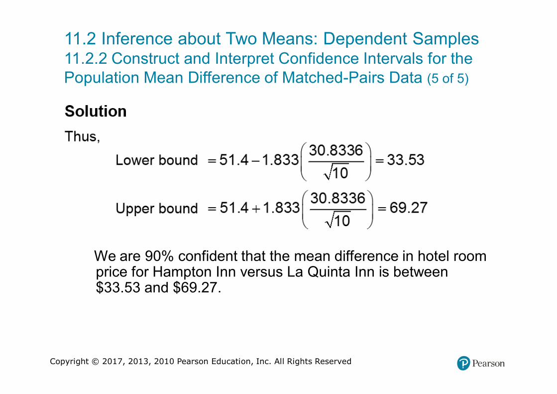
11.2 Inference about Two Means: Dependent Samples11.2.2 Construct and Interpret Confidence Intervals for the Population Mean Difference of Matched-Pairs Data (1 of 5)
Confidence Interval for Matched-Pairs Data
A (1 − α) • 100% confidence interval for μd is given by

Copyright © 2017, 2013, 2010 Pearson Education, Inc. All Rights Reserved
11.2 Inference about Two Means: Dependent Samples11.2.2 Construct and Interpret Confidence Intervals for the Population Mean Difference of Matched-Pairs Data (2 of 5)
Confidence Interval for Matched-Pairs Data
Note: The interval is exact when the population is normally distributed and approximately correct for nonnormal populations, provided that n is large.

Copyright © 2017, 2013, 2010 Pearson Education, Inc. All Rights Reserved
11.2 Inference about Two Means: Dependent Samples11.2.2 Construct and Interpret Confidence Intervals for the Population Mean Difference of Matched-Pairs Data (3 of 5)
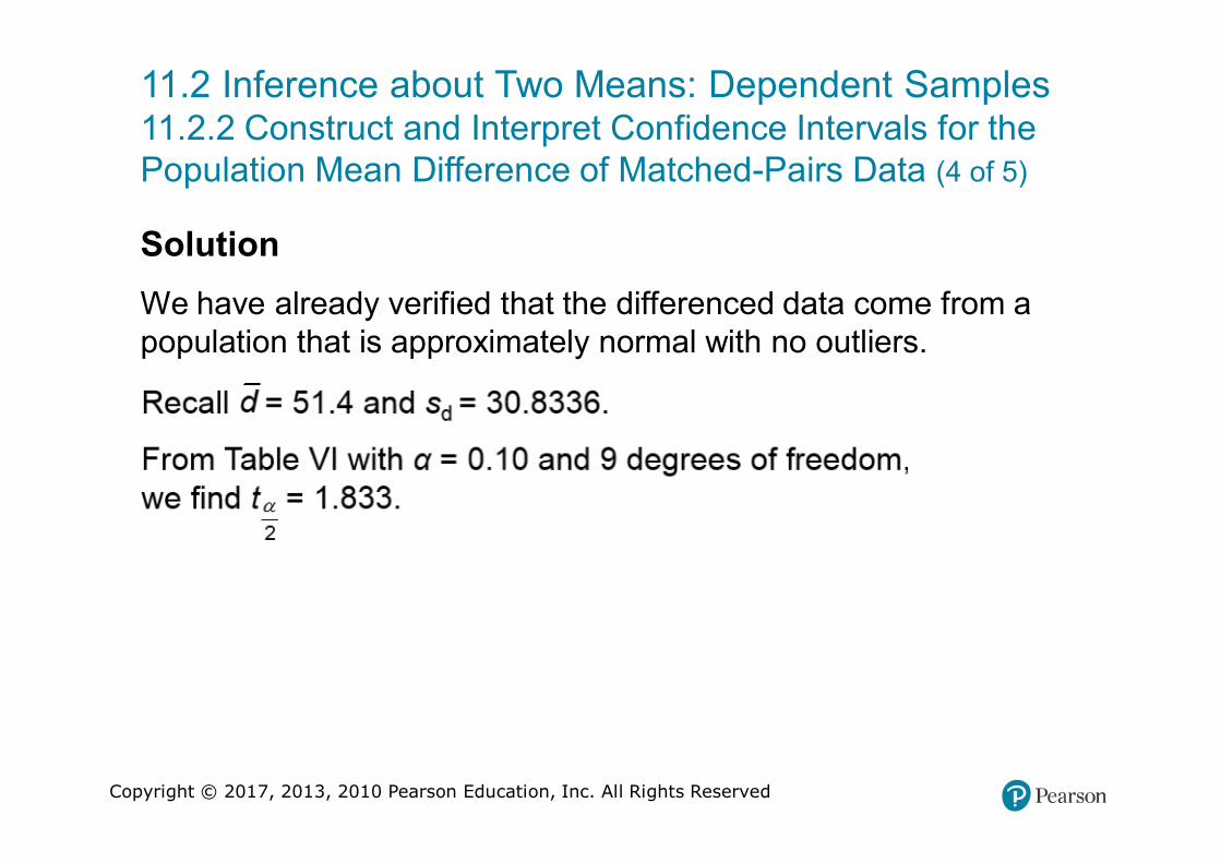
Parallel Example 4: Constructing a Confidence Interval for Matched-Pairs Data
Construct a 90% confidence interval for the mean difference in price of Hampton Inn versus La Quinta hotel rooms.
Copyright © 2017, 2013, 2010 Pearson Education, Inc. All Rights Reserved
11.2 Inference about Two Means: Dependent Samples11.2.2 Construct and Interpret Confidence Intervals for the Population Mean Difference of Matched-Pairs Data (4 of 5)
Solution
We have already verified that the differenced data come from a population that is approximately normal with no outliers.
Copyright © 2017, 2013, 2010 Pearson Education, Inc. All Rights Reserved
11.2 Inference about Two Means: Dependent Samples11.2.2 Construct and Interpret Confidence Intervals for the Population Mean Difference of Matched-Pairs Data (5 of 5)
We are 90% confident that the mean difference in hotel room price for Hampton Inn versus La Quinta Inn is between $33.53 and $69.27.

Copyright © 2017, 2013, 2010 Pearson Education, Inc. All Rights Reserved
11.3 Inference about Two Means: Independent SamplesLearning Objectives
1. Test hypotheses regarding the difference of two independent means
2. Construct and interpret confidence intervals regarding the difference of two independent means
Copyright © 2017, 2013, 2010 Pearson Education, Inc. All Rights Reserved
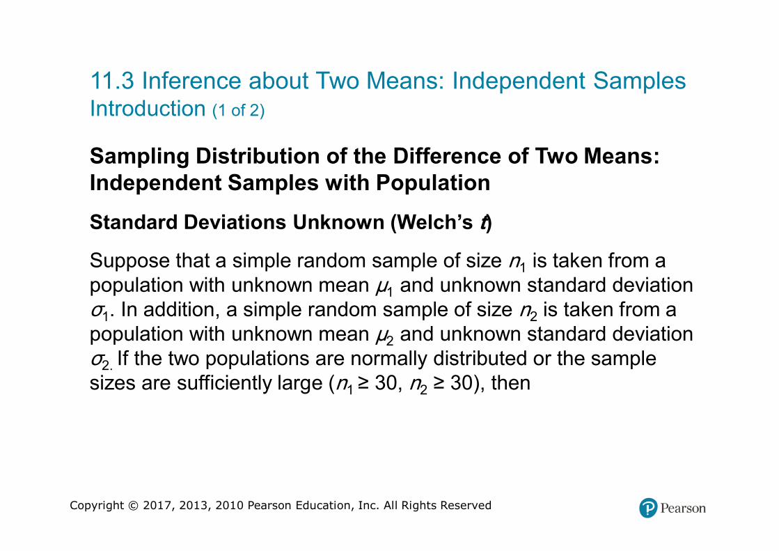
11.3 Inference about Two Means: Independent SamplesIntroduction (1 of 2)
Sampling Distribution of the Difference of Two Means: Independent Samples with Population
Standard Deviations Unknown (Welch’s t)
Suppose that a simple random sample of size n1 is taken from a population with unknown mean μ1 and unknown standard deviation σ1. In addition, a simple random sample of size n2 is taken from a population with unknown mean μ2 and unknown standard deviation σ2. If the two populations are normally distributed or the sample sizes are sufficiently large (n1 ≥ 30, n2 ≥ 30), then

Copyright © 2017, 2013, 2010 Pearson Education, Inc. All Rights Reserved
11.3 Inference about Two Means: Independent SamplesIntroduction (2 of 2)
Sampling Distribution of the Difference of Two Means: Independent Samples with Population
Standard Deviations Unknown (Welch’s t)
Copyright © 2017, 2013, 2010 Pearson Education, Inc. All Rights Reserved
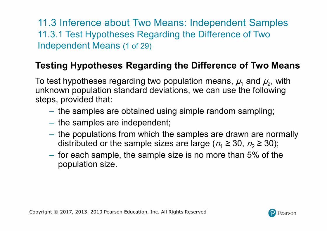
11.3 Inference about Two Means: Independent Samples11.3.1 Test Hypotheses Regarding the Difference of Two Independent Means (1 of 29)
Testing Hypotheses Regarding the Difference of Two Means
To test hypotheses regarding two population means, μ1 and μ2, with unknown population standard deviations, we can use the following steps, provided that:
– the samples are obtained using simple random sampling;
– the samples are independent;
– the populations from which the samples are drawn are normally distributed or the sample sizes are large (n1 ≥ 30, n2 ≥ 30);
– for each sample, the sample size is no more than 5% of the population size.

Copyright © 2017, 2013, 2010 Pearson Education, Inc. All Rights Reserved
11.3 Inference about Two Means: Independent Samples11.3.1 Test Hypotheses Regarding the Difference of Two Independent Means (2 of 29)
Step 1: Determine the null and alternative hypotheses. The hypotheses are structured in one of three ways:
Two-Tailed Left-Tailed Right-Tailed
H0: µ1 = µ2 H0: µ1 = µ2 H0: µ1 = µ2
H1: µ1 ≠ µ2 H1: µ1 < µ2 H1: µ1 > µ2
Note: µ1 is the population mean for population 1, and µ2 is the population mean for population 2.

Copyright © 2017, 2013, 2010 Pearson Education, Inc. All Rights Reserved
11.3 Inference about Two Means: Independent Samples11.3.1 Test Hypotheses Regarding the Difference of Two Independent Means (3 of 29)
Step 2: Select a level of significance, α, depending on the seriousness of making a Type I error.

Copyright © 2017, 2013, 2010 Pearson Education, Inc. All Rights Reserved
11.3 Inference about Two Means: Independent Samples11.3.1 Test Hypotheses Regarding the Difference of Two Independent Means (4 of 29)
Classical Approach
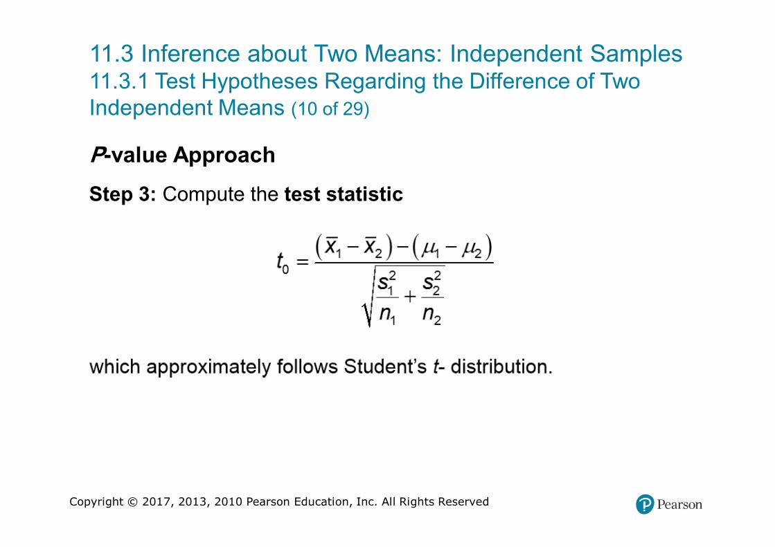
Step 3: Compute the test statistic

Copyright © 2017, 2013, 2010 Pearson Education, Inc. All Rights Reserved
11.3 Inference about Two Means: Independent Samples11.3.1 Test Hypotheses Regarding the Difference of Two Independent Means (5 of 29)
Classical Approach
Use Table VII to determine the critical value using the smaller of n1 − 1 or n2 − 1 degrees of freedom.

Copyright © 2017, 2013, 2010 Pearson Education, Inc. All Rights Reserved
11.3 Inference about Two Means: Independent Samples11.3.1 Test Hypotheses Regarding the Difference of Two Independent Means (6 of 29)
Classical Approach
Two-Tailed

Copyright © 2017, 2013, 2010 Pearson Education, Inc. All Rights Reserved
11.3 Inference about Two Means: Independent Samples11.3.1 Test Hypotheses Regarding the Difference of Two Independent Means (7 of 29)
Classical Approach
Left-Tailed
Copyright © 2017, 2013, 2010 Pearson Education, Inc. All Rights Reserved
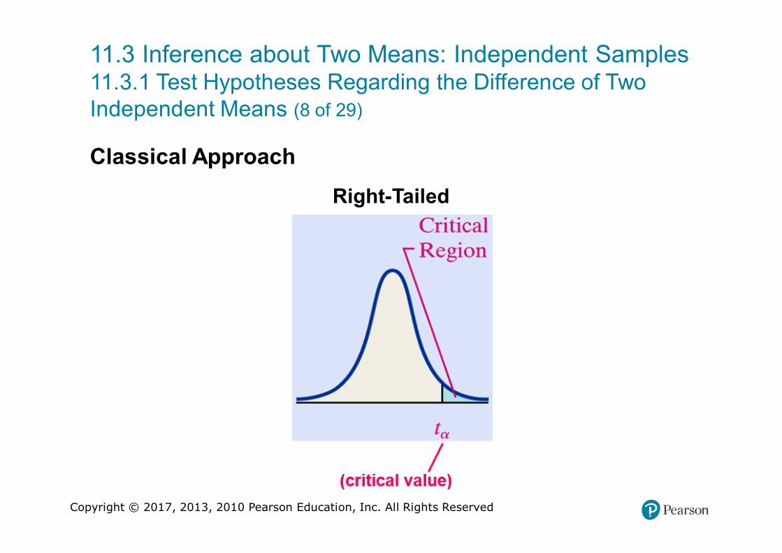
11.3 Inference about Two Means: Independent Samples11.3.1 Test Hypotheses Regarding the Difference of Two Independent Means (8 of 29)
Classical Approach
Right-Tailed

Copyright © 2017, 2013, 2010 Pearson Education, Inc. All Rights Reserved
11.3 Inference about Two Means: Independent Samples11.3.1 Test Hypotheses Regarding the Difference of Two Independent Means (9 of 29)
Classical Approach
Step 4: Compare the critical value with the test statistic:
Copyright © 2017, 2013, 2010 Pearson Education, Inc. All Rights Reserved
11.3 Inference about Two Means: Independent Samples11.3.1 Test Hypotheses Regarding the Difference of Two Independent Means (10 of 29)
P-value Approach
Step 3: Compute the test statistic

Copyright © 2017, 2013, 2010 Pearson Education, Inc. All Rights Reserved
11.3 Inference about Two Means: Independent Samples11.3.1 Test Hypotheses Regarding the Difference of Two Independent Means (11 of 29)
P-value Approach
Use Table VII to determine the P-value using the smaller of n1 − 1 or n2 − 1 degrees of freedom.

Copyright © 2017, 2013, 2010 Pearson Education, Inc. All Rights Reserved
11.3 Inference about Two Means: Independent Samples11.3.1 Test Hypotheses Regarding the Difference of Two Independent Means (12 of 29)
P-value Approach
Two-Tailed

Copyright © 2017, 2013, 2010 Pearson Education, Inc. All Rights Reserved
11.3 Inference about Two Means: Independent Samples11.3.1 Test Hypotheses Regarding the Difference of Two Independent Means (13 of 29)
P-value Approach
Left-Tailed
Copyright © 2017, 2013, 2010 Pearson Education, Inc. All Rights Reserved
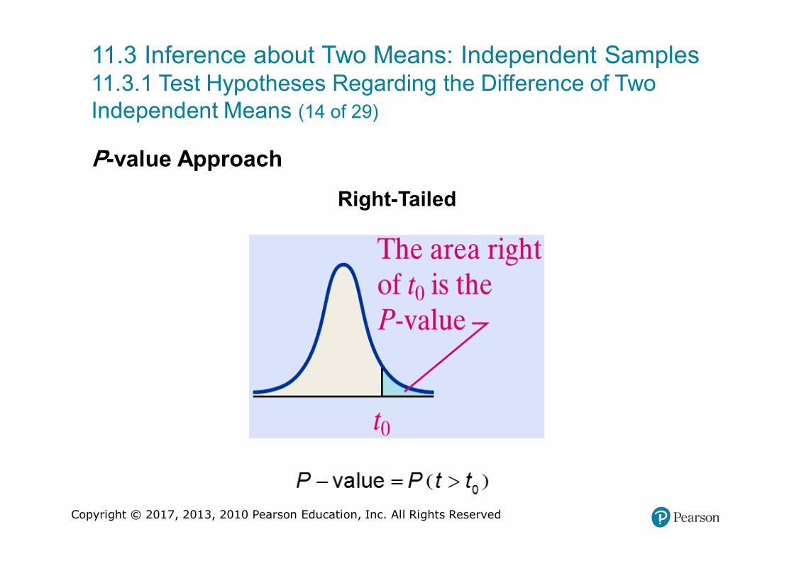
11.3 Inference about Two Means: Independent Samples11.3.1 Test Hypotheses Regarding the Difference of Two Independent Means (14 of 29)
P-value Approach
Right-Tailed

Copyright © 2017, 2013, 2010 Pearson Education, Inc. All Rights Reserved
11.3 Inference about Two Means: Independent Samples11.3.1 Test Hypotheses Regarding the Difference of Two Independent Means (15 of 29)
P-value Approach
Technology Step 3: Use a statistical spreadsheet or calculator with statistical capabilities to obtain the P-value. The directions for obtaining the P-value using the TI-83/84 Plus graphing calculator, Excel, MINITAB, and StatCrunch are in the Technology Step-by-Step in the text.

Copyright © 2017, 2013, 2010 Pearson Education, Inc. All Rights Reserved
11.3 Inference about Two Means: Independent Samples11.3.1 Test Hypotheses Regarding the Difference of Two Independent Means (16 of 29)
P-value Approach
Step 4: If P-value < α, reject the null hypothesis.

Copyright © 2017, 2013, 2010 Pearson Education, Inc. All Rights Reserved
11.3 Inference about Two Means: Independent Samples11.3.1 Test Hypotheses Regarding the Difference of Two Independent Means (17 of 29)
P-value Approach
Step 5: State the conclusion.

Copyright © 2017, 2013, 2010 Pearson Education, Inc. All Rights Reserved
11.3 Inference about Two Means: Independent Samples11.3.1 Test Hypotheses Regarding the Difference of Two Independent Means (18 of 29)
These procedures are robust, which means that minor departures from normality will not adversely affect the results. However, if the data have outliers, the procedure should not be used.

Copyright © 2017, 2013, 2010 Pearson Education, Inc. All Rights Reserved
11.3 Inference about Two Means: Independent Samples11.3.1 Test Hypotheses Regarding the Difference of Two Independent Means (19 of 29)
Parallel Example 1: Testing Hypotheses Regarding Two Means
A researcher wanted to know whether “state” quarters had a weight that is more than “traditional” quarters. He randomly selected 18 “state” quarters and 16 “traditional” quarters, weighed each of them and obtained the following data.
Copyright © 2017, 2013, 2010 Pearson Education, Inc. All Rights Reserved
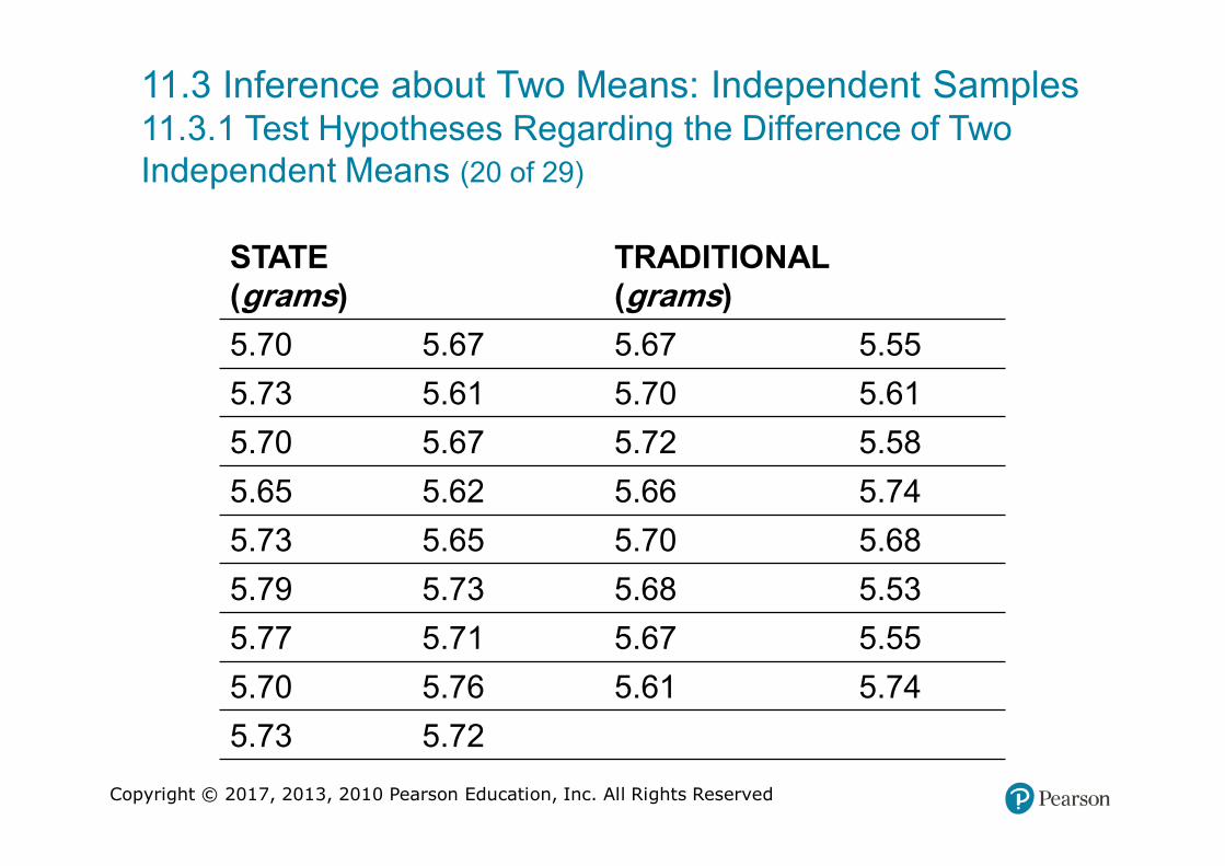
11.3 Inference about Two Means: Independent Samples11.3.1 Test Hypotheses Regarding the Difference of Two Independent Means (20 of 29)
STATE(grams)
blank TRADITIONAL(grams)
blank
5.70 5.67 5.67 5.55
5.73 5.61 5.70 5.61
5.70 5.67 5.72 5.58
5.65 5.62 5.66 5.74
5.73 5.65 5.70 5.68
5.79 5.73 5.68 5.53
5.77 5.71 5.67 5.55
5.70 5.76 5.61 5.74
5.73 5.72 blank blank

Copyright © 2017, 2013, 2010 Pearson Education, Inc. All Rights Reserved
11.3 Inference about Two Means: Independent Samples11.3.1 Test Hypotheses Regarding the Difference of Two Independent Means (21 of 29)
Test the claim that “state” quarters have a mean weight that is more than “traditional” quarters at the α = 0.05 level of significance.
NOTE: A normal probability plot of “state” quarters indicates the population could be normal. A normal probability plot of “traditional” quarters indicates the population could be normal

Copyright © 2017, 2013, 2010 Pearson Education, Inc. All Rights Reserved
11.3 Inference about Two Means: Independent Samples11.3.1 Test Hypotheses Regarding the Difference of Two Independent Means (22 of 29)
No outliers.

Copyright © 2017, 2013, 2010 Pearson Education, Inc. All Rights Reserved
11.3 Inference about Two Means: Independent Samples11.3.1 Test Hypotheses Regarding the Difference of Two Independent Means (23 of 29)
Solution
Step 1: We want to determine whether state quarters weigh more than traditional quarters:
H0: μ1 = μ2 versus H1: μ1 > μ2
Step 2: The level of significance is α = 0.05.
Step 3: The test statistic is

Copyright © 2017, 2013, 2010 Pearson Education, Inc. All Rights Reserved
11.3 Inference about Two Means: Independent Samples11.3.1 Test Hypotheses Regarding the Difference of Two Independent Means (24 of 29)
Solution: Classical Approach
This is a right-tailed test with α = 0.05. Since n1 − 1 = 17 and n2 − 1 = 15, we will use 15 degrees of freedom. The corresponding critical value is t0.05 = 1.753.

Copyright © 2017, 2013, 2010 Pearson Education, Inc. All Rights Reserved
11.3 Inference about Two Means: Independent Samples11.3.1 Test Hypotheses Regarding the Difference of Two Independent Means (25 of 29)
Solution: Classical Approach
Step 4: Since the test statistic, t0 = 2.53 is greater than the critical value t.05 = 1.753, we reject the null hypothesis.

Copyright © 2017, 2013, 2010 Pearson Education, Inc. All Rights Reserved
11.3 Inference about Two Means: Independent Samples11.3.1 Test Hypotheses Regarding the Difference of Two Independent Means (26 of 29)
Solution: P-value Approach
Because this is a right-tailed test, the P-value is the area under the t-distribution to the right of the test statistict0 = 2.53. That is, P-value = P(t > 2.53) ≈ 0.01.

Copyright © 2017, 2013, 2010 Pearson Education, Inc. All Rights Reserved
11.3 Inference about Two Means: Independent Samples11.3.1 Test Hypotheses Regarding the Difference of Two Independent Means (27 of 29)
Solution: P-value Approach
Step 4: Since the P-value is less than the level of significance α = 0.05, we reject the null hypothesis.

Copyright © 2017, 2013, 2010 Pearson Education, Inc. All Rights Reserved
11.3 Inference about Two Means: Independent Samples11.3.1 Test Hypotheses Regarding the Difference of Two Independent Means (28 of 29)
Solution
Step 5: There is sufficient evidence at the α = 0.05 level to conclude that the state quarters weigh more than the traditional quarters.

Copyright © 2017, 2013, 2010 Pearson Education, Inc. All Rights Reserved
11.3 Inference about Two Means: Independent Samples11.3.1 Test Hypotheses Regarding the Difference of Two Independent Means (29 of 29)
NOTE: The degrees of freedom used to determine the critical value in the last example are conservative. Results that are more accurate can be obtained by using the following degrees of freedom:

Copyright © 2017, 2013, 2010 Pearson Education, Inc. All Rights Reserved
11.3 Inference about Two Means: Independent Samples11.3.2 Construct and Interpret Confidence Intervals Regarding the Difference of Two Independent Means (1 of 8)
Constructing a (1 − α) • 100% Confidence Interval for the Difference of Two Means
A simple random sample of size n1 is taken from a population with unknown mean μ1 and unknown standard deviation σ1. Also, a simple random sample of size n2 is taken from a population with unknown mean μ2 and unknown standard deviation σ2. If the two populations are normally distributed or the sample sizes are sufficiently large (n1 ≥ 30 and n2 ≥ 30), a(1 − α) • 100% confidence interval about μ1 − μ2 is given by . . .

Copyright © 2017, 2013, 2010 Pearson Education, Inc. All Rights Reserved
11.3 Inference about Two Means: Independent Samples11.3.2 Construct and Interpret Confidence Intervals Regarding the Difference of Two Independent Means (2 of 8)
Constructing a (1 − α) • 100% Confidence Interval for the Difference of Two Means

Copyright © 2017, 2013, 2010 Pearson Education, Inc. All Rights Reserved
11.3 Inference about Two Means: Independent Samples11.3.2 Construct and Interpret Confidence Intervals Regarding the Difference of Two Independent Means (3 of 8)
Parallel Example 3: Constructing a Confidence Interval for the Difference of Two Means
Construct a 95% confidence interval about the difference between the population mean weight of a “state” quarter versus the population mean weight of a “traditional” quarter.
Copyright © 2017, 2013, 2010 Pearson Education, Inc. All Rights Reserved
11.3 Inference about Two Means: Independent Samples11.3.2 Construct and Interpret Confidence Intervals Regarding the Difference of Two Independent Means (4 of 8)
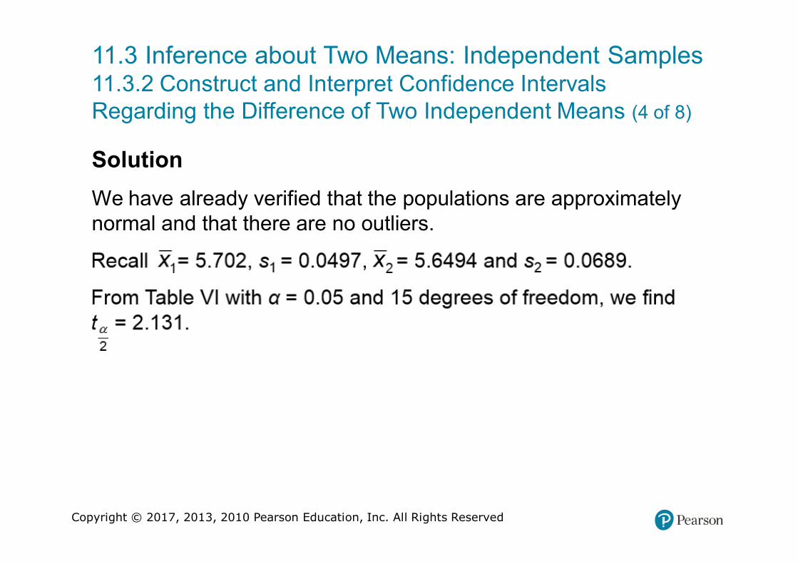
Solution
We have already verified that the populations are approximately normal and that there are no outliers.

Copyright © 2017, 2013, 2010 Pearson Education, Inc. All Rights Reserved
11.3 Inference about Two Means: Independent Samples11.3.2 Construct and Interpret Confidence Intervals Regarding the Difference of Two Independent Means (5 of 8)
Solution
Thus,
Copyright © 2017, 2013, 2010 Pearson Education, Inc. All Rights Reserved
11.3 Inference about Two Means: Independent Samples11.3.2 Construct and Interpret Confidence Intervals Regarding the Difference of Two Independent Means (6 of 8)
Solution
We are 95% confident that the mean weight of the “state” quarters is between 0.0086 and 0.0974 ounces more than the mean weight of the “traditional” quarters. Since the confidence interval does not contain 0, we conclude that the “state” quarters weigh more than the “traditional” quarters.

Copyright © 2017, 2013, 2010 Pearson Education, Inc. All Rights Reserved
11.3 Inference about Two Means: Independent Samples11.3.2 Construct and Interpret Confidence Intervals Regarding the Difference of Two Independent Means (7 of 8)
When the population variances are assumed to be equal, the pooled t-statistic can be used to test for a difference in means for two independent samples. The pooled t-statistic is computed by finding a weighted average of the sample variances and uses this average in the computation of the test statistic.
The advantage of this test statistic is that it exactly follows Student’s t-distribution with n1 + n2 − 2 degrees of freedom.
The disadvantage to this test statistic is that it requires that the population variances be equal.

Copyright © 2017, 2013, 2010 Pearson Education, Inc. All Rights Reserved
11.3 Inference about Two Means: Independent Samples11.3.2 Construct and Interpret Confidence Intervals Regarding the Difference of Two Independent Means (8 of 8)
CAUTION!
We would use the pooled two-sample t-test when the two samples come from populations that have the same variance. Pooling refers to finding a weighted average of the two sample variances from the independent samples. It is difficult to verify that two population variances might be equal based on sample data, so we will always use Welch’s t when comparing two means.

Copyright © 2017, 2013, 2010 Pearson Education, Inc. All Rights Reserved
11.4 Inference about Two Population Standard DeviationsLearning Objectives
1. Find critical values of the F-distribution
2. Test hypotheses regarding two population standard deviations

Copyright © 2017, 2013, 2010 Pearson Education, Inc. All Rights Reserved
11.4 Inference about Two Population Standard Deviations11.4.1 Find Critical Values of the F-distribution (1 of 11)
Requirements for Testing Claims Regarding Two Population Standard Deviations
1. The samples are independent simple random samples or from a completely randomized design.
2. The populations from which the samples are drawn are normally distributed.

Copyright © 2017, 2013, 2010 Pearson Education, Inc. All Rights Reserved
11.4 Inference about Two Population Standard Deviations11.4.1 Find Critical Values of the F-distribution (2 of 11)
CAUTION!
If the populations from which the samples are drawn are not normal, do not use the inferential procedures discussed in this section.

Copyright © 2017, 2013, 2010 Pearson Education, Inc. All Rights Reserved
11.4 Inference about Two Population Standard Deviations11.4.1 Find Critical Values of the F-distribution (3 of 11)
Notation Used When Comparing Two Population Standard Deviations

Copyright © 2017, 2013, 2010 Pearson Education, Inc. All Rights Reserved
11.4 Inference about Two Population Standard Deviations11.4.1 Find Critical Values of the F-distribution (4 of 11)
follows the F-distribution with n1 − 1 degrees of freedom in the numerator and n2 − 1 degrees of freedom in the denominator.

Copyright © 2017, 2013, 2010 Pearson Education, Inc. All Rights Reserved
11.4 Inference about Two Population Standard Deviations11.4.1 Find Critical Values of the F-distribution (5 of 11)
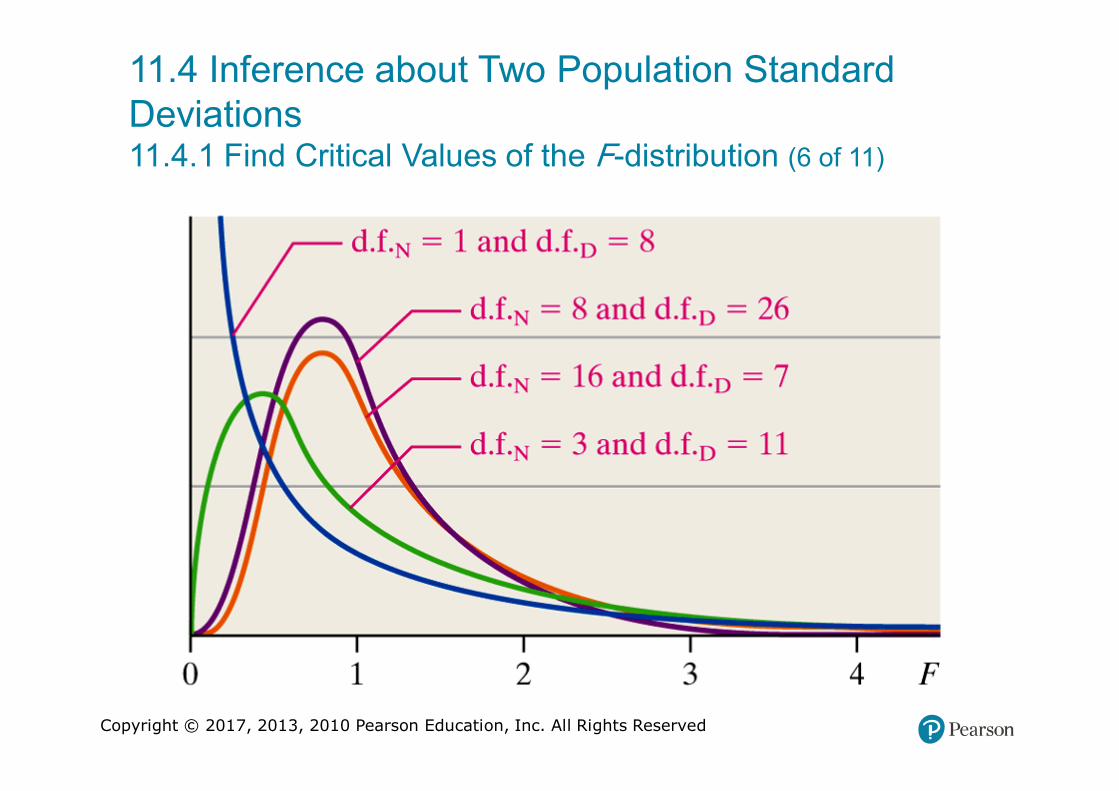
Characteristics of the F-distribution
1. It is not symmetric. The F-distribution is skewed right.
2. The shape of the F-distribution depends upon the degrees of freedom in the numerator and denominator. This is similar to the χ2 distribution and Student’s t-distribution, whose shape depends upon their degrees of freedom.
3. The total area under the curve is 1.
4. The values of F are always greater than or equal to zero.
Copyright © 2017, 2013, 2010 Pearson Education, Inc. All Rights Reserved
11.4 Inference about Two Population Standard Deviations11.4.1 Find Critical Values of the F-distribution (6 of 11)

Copyright © 2017, 2013, 2010 Pearson Education, Inc. All Rights Reserved
11.4 Inference about Two Population Standard Deviations11.4.1 Find Critical Values of the F-distribution (7 of 11)
is the critical F with n1 − 1 degrees of freedom in the numerator and n2 − 1 degrees of freedom in the denominator and an area of α to the right of the critical F.

Copyright © 2017, 2013, 2010 Pearson Education, Inc. All Rights Reserved
11.4 Inference about Two Population Standard Deviations11.4.1 Find Critical Values of the F-distribution (8 of 11)
To determine the critical value that has an area of α to the left, use the following property:

Copyright © 2017, 2013, 2010 Pearson Education, Inc. All Rights Reserved
11.4 Inference about Two Population Standard Deviations11.4.1 Find Critical Values of the F-distribution (9 of 11)
Parallel Example 1: Finding Critical Values for the F-distribution
Find the critical F-value:
a) for a right-tailed test with α = 0.1, degrees of freedom in the numerator = 8 and degrees of freedom in the denominator = 4.
b) for a two-tailed test with α = 0.05, degrees of freedom in the numerator = 20 and degrees of freedom in the denominator = 15.

Copyright © 2017, 2013, 2010 Pearson Education, Inc. All Rights Reserved
11.4 Inference about Two Population Standard Deviations11.4.1 Find Critical Values of the F-distribution (10 of 11)
Solution
a) F0.1, 8, 4 = 3.95
b) F.025, 20, 15 = 2.76
Copyright © 2017, 2013, 2010 Pearson Education, Inc. All Rights Reserved
11.4 Inference about Two Population Standard Deviations11.4.1 Find Critical Values of the F-distribution (11 of 11)
NOTE:
If the number of degrees of freedom is not found in the table, we follow the practice of choosing the degrees of freedom closest to that desired. If the degrees of freedom is exactly between two values, find the mean of the values.

Copyright © 2017, 2013, 2010 Pearson Education, Inc. All Rights Reserved
11.4 Inference about Two Population Standard Deviations11.4.2 Test Hypotheses Regarding Two Population Standard Deviations (1 of 22)
Test Hypotheses Regarding Two Population Standard Deviations
To test hypotheses regarding two population standard deviations, σ1 and σ2, we can use the following steps, provided that
1. the samples are obtained using simple random sampling.
2. the sample data are independent.
3. the populations from which the samples are drawn are normally distributed.

Copyright © 2017, 2013, 2010 Pearson Education, Inc. All Rights Reserved
11.4 Inference about Two Population Standard Deviations11.4.2 Test Hypotheses Regarding Two Population Standard Deviations (2 of 22)
Step 1: Determine the null and alternative hypotheses. The hypotheses can be structured in one of three ways:
Two-Tailed Left-Tailed Right-Tailed
H0: σ1 = σ2 H0: σ1 = σ2 H0: σ1 = σ2
H1: σ1 ≠ σ2 H1: σ1 < σ2 H1: σ1 > σ2

Copyright © 2017, 2013, 2010 Pearson Education, Inc. All Rights Reserved
11.4 Inference about Two Population Standard Deviations11.4.2 Test Hypotheses Regarding Two Population Standard Deviations (3 of 22)
Step 2: Select a level of significance, α, depending on the seriousness of making a Type I error.

Copyright © 2017, 2013, 2010 Pearson Education, Inc. All Rights Reserved
11.4 Inference about Two Population Standard Deviations11.4.2 Test Hypotheses Regarding Two Population Standard Deviations (4 of 22)
which follows Fisher’s F-distribution with n1 − 1 degrees of freedom in the numerator and n2 − 1 degrees of freedom in the denominator.

Copyright © 2017, 2013, 2010 Pearson Education, Inc. All Rights Reserved
11.4 Inference about Two Population Standard Deviations11.4.2 Test Hypotheses Regarding Two Population Standard Deviations (5 of 22)
Classical Approach
Use Table IX to determine the critical value(s) using n1 − 1 degrees of freedom in the numerator and n2 − 1 degrees of freedom in the denominator. The shaded regions in the graphs on the following slides represent the critical regions.

Copyright © 2017, 2013, 2010 Pearson Education, Inc. All Rights Reserved
11.4 Inference about Two Population Standard Deviations11.4.2 Test Hypotheses Regarding Two Population Standard Deviations (6 of 22)
Classical Approach
Two-Tailed

Copyright © 2017, 2013, 2010 Pearson Education, Inc. All Rights Reserved
11.4 Inference about Two Population Standard Deviations11.4.2 Test Hypotheses Regarding Two Population Standard Deviations (7 of 22)
Classical Approach
Left-Tailed

Copyright © 2017, 2013, 2010 Pearson Education, Inc. All Rights Reserved
11.4 Inference about Two Population Standard Deviations11.4.2 Test Hypotheses Regarding Two Population Standard Deviations (8 of 22)
Classical Approach
Right-Tailed

Copyright © 2017, 2013, 2010 Pearson Education, Inc. All Rights Reserved
11.4 Inference about Two Population Standard Deviations11.4.2 Test Hypotheses Regarding Two Population Standard Deviations (9 of 22)
Classical Approach
Step 4: Compare the critical value with the test statistic:

Copyright © 2017, 2013, 2010 Pearson Education, Inc. All Rights Reserved
11.4 Inference about Two Population Standard Deviations11.4.2 Test Hypotheses Regarding Two Population Standard Deviations (10 of 22)
P-value Approach
Step 3: Use technology to determine the P-value.

Copyright © 2017, 2013, 2010 Pearson Education, Inc. All Rights Reserved
11.4 Inference about Two Population Standard Deviations11.4.2 Test Hypotheses Regarding Two Population Standard Deviations (11 of 22)
P-value Approach
Step 4: If P-value < α, reject the null hypothesis.

Copyright © 2017, 2013, 2010 Pearson Education, Inc. All Rights Reserved
11.4 Inference about Two Population Standard Deviations11.4.2 Test Hypotheses Regarding Two Population Standard Deviations (12 of 22)
P-value Approach
Step 5: State the conclusion.
Copyright © 2017, 2013, 2010 Pearson Education, Inc. All Rights Reserved
11.4 Inference about Two Population Standard Deviations11.4.2 Test Hypotheses Regarding Two Population Standard Deviations (13 of 22)
CAUTION!
The test for equality of population standard deviations is not robust. Thus, any departures from normality make the results of the inference useless.
Copyright © 2017, 2013, 2010 Pearson Education, Inc. All Rights Reserved
11.4 Inference about Two Population Standard Deviations11.4.2 Test Hypotheses Regarding Two Population Standard Deviations (14 of 22)
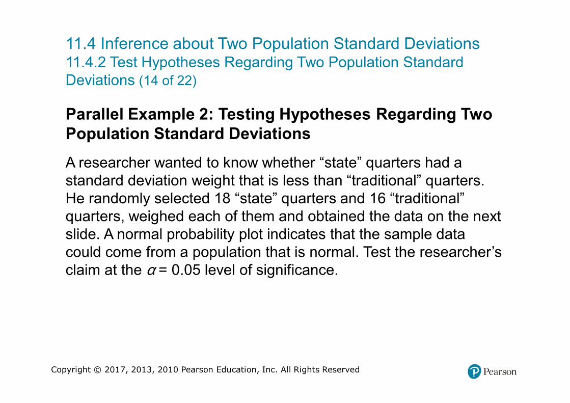
Parallel Example 2: Testing Hypotheses Regarding Two Population Standard Deviations
A researcher wanted to know whether “state” quarters had a standard deviation weight that is less than “traditional” quarters. He randomly selected 18 “state” quarters and 16 “traditional”quarters, weighed each of them and obtained the data on the next slide. A normal probability plot indicates that the sample data could come from a population that is normal. Test the researcher’s claim at the α = 0.05 level of significance.

Copyright © 2017, 2013, 2010 Pearson Education, Inc. All Rights Reserved
11.4 Inference about Two Population Standard Deviations11.4.2 Test Hypotheses Regarding Two Population Standard Deviations (15 of 22)
STATE(grams)
blank TRADITIONAL(grams)
blank
5.70 5.67 5.67 5.55
5.73 5.61 5.70 5.61
5.70 5.67 5.72 5.58
5.65 5.62 5.66 5.74
5.73 5.65 5.70 5.68
5.79 5.73 5.68 5.53
5.77 5.71 5.67 5.55
5.70 5.76 5.61 5.74
5.73 5.72 blank blank
Copyright © 2017, 2013, 2010 Pearson Education, Inc. All Rights Reserved
11.4 Inference about Two Population Standard Deviations11.4.2 Test Hypotheses Regarding Two Population Standard Deviations (16 of 22)
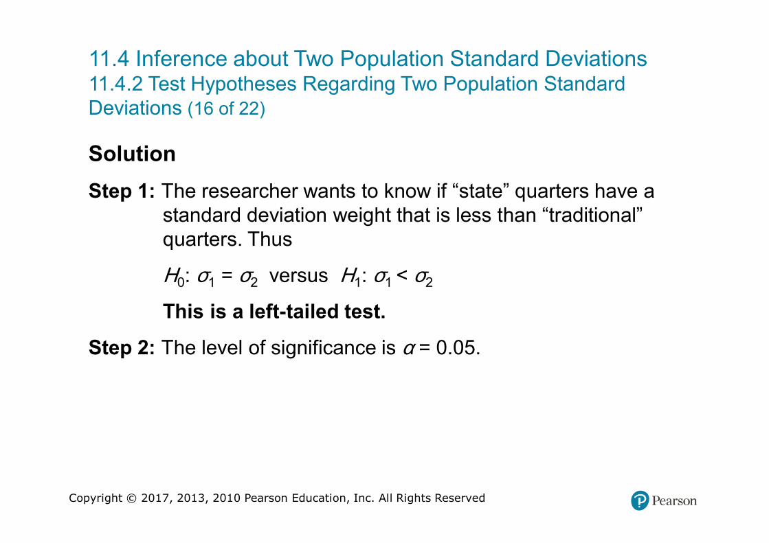
Solution
Step 1: The researcher wants to know if “state” quarters have a standard deviation weight that is less than “traditional”quarters. Thus
H0: σ1 = σ2 versus H1: σ1 < σ2
This is a left-tailed test.
Step 2: The level of significance is α = 0.05.

Copyright © 2017, 2013, 2010 Pearson Education, Inc. All Rights Reserved
11.4 Inference about Two Population Standard Deviations11.4.2 Test Hypotheses Regarding Two Population Standard Deviations (17 of 22)
Solution
Step 3: The standard deviation of “state” quarters was found to be 0.0497 and the standard deviation of “traditional” quarters was found to be 0.0689. The test statistic is then

Copyright © 2017, 2013, 2010 Pearson Education, Inc. All Rights Reserved
11.4 Inference about Two Population Standard Deviations11.4.2 Test Hypotheses Regarding Two Population Standard Deviations (18 of 22)
Solution: Classical Approach
Since this is a left-tailed test, we determine the critical value at the 1 − α = 1 − 0.05 = 0.95 level of significance with n1 − 1 = 18 − 1 = 17 degrees of freedom in the numerator and n2 − 1 = 16 − 1 = 15 degrees of freedom in the denominator. Thus,

Copyright © 2017, 2013, 2010 Pearson Education, Inc. All Rights Reserved
11.4 Inference about Two Population Standard Deviations11.4.2 Test Hypotheses Regarding Two Population Standard Deviations (19 of 22)
Solution: Classical Approach
Step 4: Since the test statistic F0 = 0.52 is greater than the critical value F0.95,17,15 = 0.42, we fail to reject the null hypothesis.

Copyright © 2017, 2013, 2010 Pearson Education, Inc. All Rights Reserved
11.4 Inference about Two Population Standard Deviations11.4.2 Test Hypotheses Regarding Two Population Standard Deviations (20 of 22)
Solution: P-value Approach
Step 3: Using technology, we find that the P-value is 0.097. If the statement in the null hypothesis were true, we would expect to get results at least as extreme as obtained about 10 out of 100 times. This is not very unusual.

Copyright © 2017, 2013, 2010 Pearson Education, Inc. All Rights Reserved
11.4 Inference about Two Population Standard Deviations11.4.2 Test Hypotheses Regarding Two Population Standard Deviations (21 of 22)
Solution: P-value Approach
Step 4: Since the P-value is greater than the level of significance, α = 0.05, we fail to reject the null hypothesis.

Copyright © 2017, 2013, 2010 Pearson Education, Inc. All Rights Reserved
11.4 Inference about Two Population Standard Deviations11.4.2 Test Hypotheses Regarding Two Population Standard Deviations (22 of 22)
Solution
Step 5: There is not enough evidence to conclude that the standard deviation of weight is less for “state” quarters than it is for “traditional” quarters at the α = 0.05 level of significance.

Copyright © 2017, 2013, 2010 Pearson Education, Inc. All Rights Reserved
11.5 Putting It Together: Which Method Do I Use?Learning Objectives
1. Determine the appropriate hypothesis test to perform
Copyright © 2017, 2013, 2010 Pearson Education, Inc. All Rights Reserved
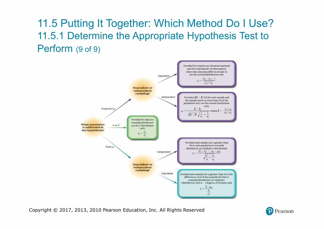
11.5 Putting It Together: Which Method Do I Use?11.5.1 Determine the Appropriate Hypothesis Test to
Perform (1 of 9)
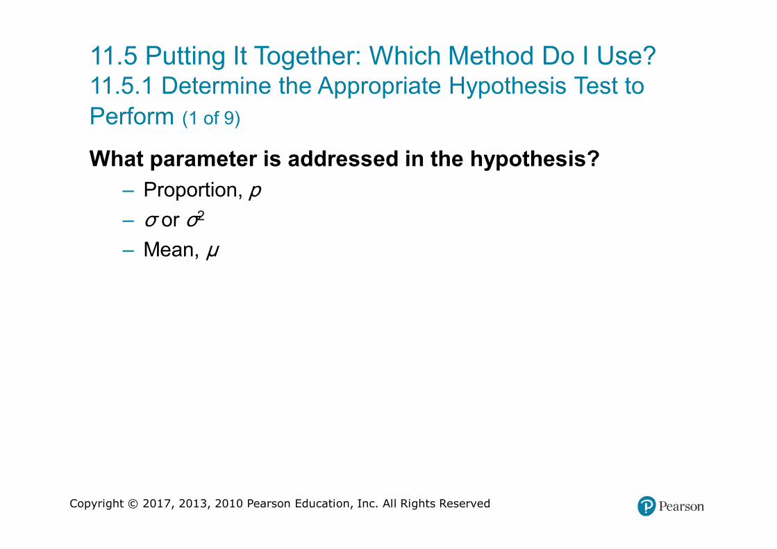
What parameter is addressed in the hypothesis?
– Proportion, p
– σ or σ2
– Mean, μ

Copyright © 2017, 2013, 2010 Pearson Education, Inc. All Rights Reserved
11.5 Putting It Together: Which Method Do I Use?11.5.1 Determine the Appropriate Hypothesis Test to
Perform (2 of 9)
Proportion, p
Is the sampling Dependent or Independent?
Copyright © 2017, 2013, 2010 Pearson Education, Inc. All Rights Reserved
11.5 Putting It Together: Which Method Do I Use?11.5.1 Determine the Appropriate Hypothesis Test to
Perform (3 of 9)
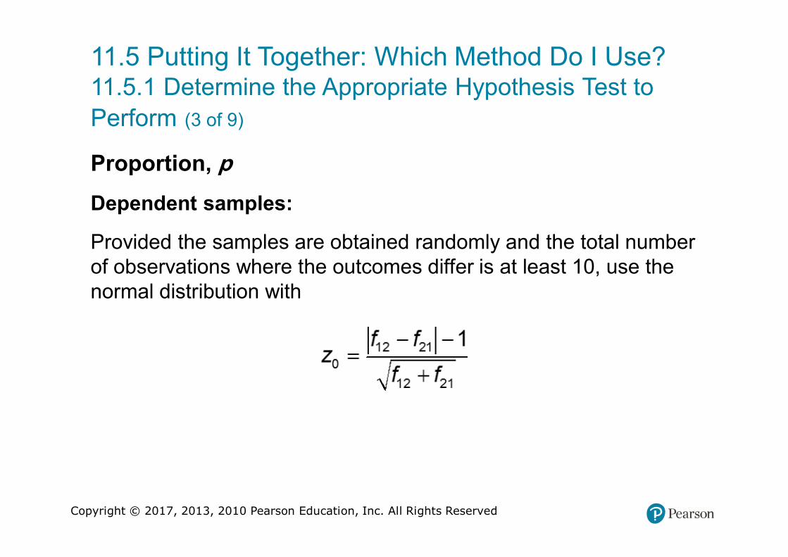
Proportion, p
Dependent samples:
Provided the samples are obtained randomly and the total number of observations where the outcomes differ is at least 10, use the normal distribution with

Copyright © 2017, 2013, 2010 Pearson Education, Inc. All Rights Reserved
11.5 Putting It Together: Which Method Do I Use?11.5.1 Determine the Appropriate Hypothesis Test to
Perform (4 of 9)
Proportion, p
Independent samples:

Copyright © 2017, 2013, 2010 Pearson Education, Inc. All Rights Reserved
11.5 Putting It Together: Which Method Do I Use?11.5.1 Determine the Appropriate Hypothesis Test to
Perform (5 of 9)
σ or σ2
Provided the data are normally distributed, use the F-distribution with

Copyright © 2017, 2013, 2010 Pearson Education, Inc. All Rights Reserved
11.5 Putting It Together: Which Method Do I Use?11.5.1 Determine the Appropriate Hypothesis Test to
Perform (6 of 9)
Mean, μ
Is the sampling Dependent or Independent?
Copyright © 2017, 2013, 2010 Pearson Education, Inc. All Rights Reserved
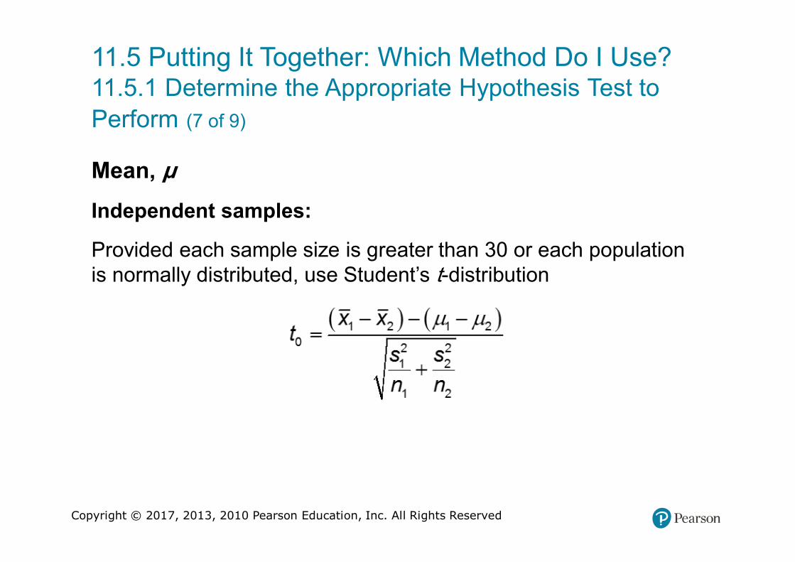
11.5 Putting It Together: Which Method Do I Use?11.5.1 Determine the Appropriate Hypothesis Test to
Perform (7 of 9)
Mean, μ
Independent samples:
Provided each sample size is greater than 30 or each population is normally distributed, use Student’s t-distribution
Copyright © 2017, 2013, 2010 Pearson Education, Inc. All Rights Reserved
11.5 Putting It Together: Which Method Do I Use?11.5.1 Determine the Appropriate Hypothesis Test to
Perform (8 of 9)
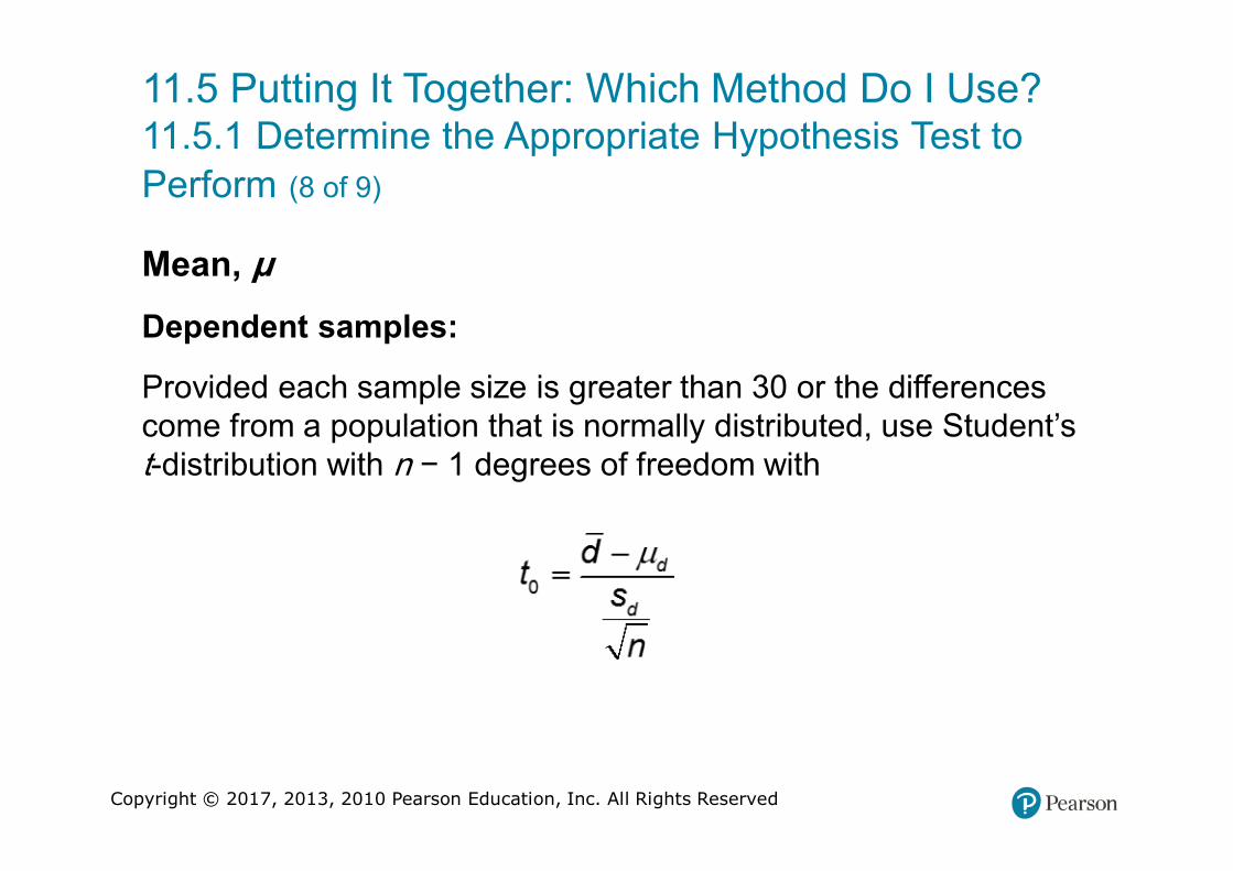
Mean, μ
Dependent samples:
Provided each sample size is greater than 30 or the differences come from a population that is normally distributed, use Student’s t-distribution with n − 1 degrees of freedom with
Copyright © 2017, 2013, 2010 Pearson Education, Inc. All Rights Reserved
11.5 Putting It Together: Which Method Do I Use?11.5.1 Determine the Appropriate Hypothesis Test to
Perform (9 of 9)