· COMPUIER-AIDED PROCESS PLANNING

AND FIXTURE DESIGN (CAPPFD)

A thesis submitted for the Degree of

Doctor of Philosophy in Mechanical Engineering

at the University of Canterbury,

Christchurch, New Zealand

by

Y ongyooth Sermsuti-Anuwat

B.Eng.(KMIT), M.Eng.Sc.(UNSW)

July 1992

ENGINEERING LIBRARY

To my wife, Prapai, and our children for their support and encouragement

ABSTRACf

This thesis describes a computer program for process planning and

fixture design. It utilizes the principles of workpiece control, in particular

dimensional and geometric control, to sequence the machining operations and

to design the 3-2-1 location systems.

The system developed uses the matrix spatial representation, a series

of two-dimensional arrays, to describe the workpiece geometry. The system is

capable of sequencing three types of .machined features requiring milling

operations: plane surfaces, slots, and steps. These features may be regarded as

two-dimensional type: they can be completely specified dimensionally in two

orthogonal projection views. Other data required by the system include the

surfaces to be machined, cutting conditions, dimensions and tolerances of the

stock and of the finished part. These data are either interactively input into

the system or stored in a prepared data file for the system to read. The

outputs include the process picture showing all locating surfaces in the 3-2-1

location system for each operation, and a set of three tolerance charts for

analysing all dimensions of the machined part.

The results of this research indicate that the automatic machining

sequence planning can be achieved through the implementation of the

concept of workpiece control together with the practicality in machining a

machined feature. The research also emphasises a significant role of the

tolerance charts which have been used in manual process planning for a long

time, but have not yet been exploited to its full advantage in computerised

process planning. Regarding tolerance charts, the research has developed a

new method for calculating tolerance stacks which can be used for

computerized as well as manual charting.

The ideas presented in the report could be applied to the systems·

using a commercial solid modelling package.

ACKNOWLEDGEMENTS

I would like to express my sincere thanks to my supervisors, Dr K.

Whybrew and Professor H. McCallion, for their invaluable aid, and guidance

throughout the course of executing the project and writing the thesis.

I also wish to extend my deep gratitude to Dr D.F. Robinson for his

advice on the use of graph theory in tolerance charting.

To my former associate supervisor, Dr G. Britton, goes a warm

gratitude for his useful discussions on various points of the research at its

early stage.

Thanks are also due to my fellow postgraduates, past and present:

Bryan Ngoi, Murray Aitkin, Mark Tunnicliffe, Kevin Hill, Colin McMurtrie

and Steve Hampson, for their help and support.

Last but not least, I would like to thank to Mr P.R. Smith, the system

analyst, who never made me disappointed whenever the need for his help

arose.

CONTENTS

1. Introduction 1

1.1 Principles of process planning 3

1.2 Literature review 11

1.3 Problems in developing CAPP and AFD systems 16

1.4 Objectives and scope of the project 17

1.5 Programming technique 19

1.6 Computer-aided process planning and

fixture design system (CAPPFD) 20

1.7 Conclusion 20

2. Tolerance chart technique 21

2.1 Tolerance charts 21

2.2 Development of tolerance chart technique

using rooted-tree graphs 23

2.3 A method of calculating working dimensions 27

2.4 Manual tolerance chart calculations 28

2.5 Computer program for tolerance charting 32

2.6 Conclusion 35

3. System structure 36

3.1 Machined features for CAPPFD 36

3.2 Structure of CAPPFD 37

3.3 CAPPFD flowchart 38

3.4 Conclusion 41

4. Data: storage, input and output 42

4.1 Spatial representation technique 42

4.2 Data structure for surface coordinates 45

4.3 Surface coordinates extraction 46

4.4 Graphical screen display 51

4.5 Production data 51

4.6 Data input 55

4.7 Data output 57

4.8 Conclusion 59

5. Machining sequence planning 60

5.1 Forward and backward planning 60

5.2 Basic sequencing concept 61

5.3 Ranking of machining operations 62

5.4 Sequence modifications 65

5.5 Adjustments for combined slots 67

5.6 Calculation of surface locating area 70

5.7 Conclusion 71

6. Location systems 72

6.1 Process picture 72

6.2 Backward planning: the application 73

6.3 Type of locating surface 74

6.4 Slot base and step base 74

6.5 Searching for locating surfaces 76

6.6 Searching for a location system 78

6.7 Graphical output of a location system 82

6.8 Workpiece model modification 83

6.9 Preparing data for the next search 85

6.10 Conclusion 88

7. Tolerance charting in CAPPFD 89

7.1 Tolerance chart module 89

7.2 Data preparation for tolerance chart module 91

7.3 Sign convention for machining cuts 97

7.4

7.5

Calculation and drawing routines

Conclusion

8. Running the CAPPFD system

8.1 ~xample 1

8.2 ~xample 2

8.3 Conclusion

9. Conclusions and recommendations

9.1 Conclusions

9.2 Recommendations for future research

References

Appendix A: A graph-theoretic approach

to tolerance charting

Appendix B: Decision table technique

Appendix C: Some results from the testing of

tolerance chart program

Appendix D: The method of traces

99

100

101

101

115

117

126

126

127

129

135

147

151

160

1

. 1. INTRODUCTION

Process planning is the activity of planning the steps of manufacturing

a product; the term is normally used in connection with metal machining.

The task of process planning may include: selecting machine-tools and

equipment to manufacture a product, planning the processing sequence,

determining the methods for positioning and holding the workpiece during

processing, specifying the appropriate cutting conditions, calculating the

standard times, and producing the operation sheets for workshop use. Its

scope may range from high level planning involving a number of machines or

processes to low level planning confined to only one machine or process, in

which the term is usually referred to as machining sequencing or operation

planning.

Because the task covers a wide range of practical activities and know­

how, process planning requires a highly skilled and experienced process

engineer who has been on the job long enough to be well versed in the use of

the machines, tools, and other auxiliary production equipment (such as jigs

and fixtures). Unfortunately, the number of people available with these

qualifications is diminishing, and it requires a long time to accumulate the

knowledge and experience necessary to be a proficient process planner. As

the batch manufacturing expands, the demand for process planners also

expands. Hence a shortage of process planners is unavoidable; this problem

has arisen in both the USA [1] and the UK [2]. In addition to the problem of

numbers, manual process planning is SUbjective, inconsistent and time­

consuming. Therefore attempts have been made to use computers to

. automate process planning. Towards the beginning of the 1980s,

computerised process planning became a research subject in institutions all

over the world. At present, Computer-Automated Process Planning, and

Computer-Aided Process Planning (CAPP) are terms in common use in both

manufacturing industry and academic engineering institutions.

2

Fixture design is another important pre-manufacturing activity which is

concerned with designing devices to position and hold the workpiece while

being machined, inspected, or assembled. In production machining, this area

of design is usually the responsibility of the tool engineer or tool designer.

The fundamental aims of using fixtures are to ensure the required degree of

interchangeability of the parts and to increase the productivity. Formerly, this

production device was known as a jig or a fixture: a jig was used in drilling

operations and had a guide for the drill; a fixture was used on the machine

where the device was moving or standing still while the processing operations

were performed on the part, but there was no guide for tools or cutters.

Nowadays, the terms are still commonly used on the shop-floor; however, in

the literature, the term 'fixture' alone is often referred to both jig and fixture

in the former context.

Like process planning, fixture design used to be regarded as an art;

good tool designers had to strive for years, working in a workshop, to acquire

the practical experience. Fortunately, the work on jig and fixture design has

been well documented; useful guidelines for practical design are available in

several books: in particular, those written by Town[3], Gates[4], Kempster[5],

Cole[6], Wilson[7] and Donaldson et al[8]. Guidelines are also made

available for an analytical approach to jig and fixture design, for example, the

book written by Hendriksen[9]. These valuable guidelines have been adopted

in industry and technical colleges for a long time. In the early 1980s,

. computers were introduced to aid fixture design; this opened up another

branch of research: Automated Fixture Design (AFD).

Process planning and fixture design are so closely related that fixture

design could be considered as a part of the whole process planning activity.

This is because the design specifications for a fixture involve the machining

sequence and the location systems for positioning the workpiece in the

processing steps. These pieces of information are the results of process

planning, and the tool designer can use them as a basis for designing or for

selecting fixturing elements: locators, supports, and clamping mechanisms.

3

In the following section, the fundamental principles of process planning

are briefly presented to describe the practical nature of this planning function,

and its interconnection with fixture design.

1.1

Although process planning has existed since metal machining

enterprises started to realise the importance of the planning activity to

achieve the organization's goals, the publications that document the procedure

for process planning are very few. Among them, the material contributed by

Lander, L.C.[10] is of most value. This small book outlines the basic steps of

process planning used in the General Motors Institute, more than 50 years

ago; probably, there, the analytical approach of process planning was first

started. The principles given in the book were later detailed by Dolye[ll],

and Eary and Johnson[12]. The discussion in this section is based heavily on

these sources and the procedure recommended by the ASTME[13].

The general steps of process planning are as follows:

(1) Analyse the part drawings

In this first step, the part drawings from product engineering are

carefully studied by the process planner with a view to facilitating and

economizing the manufacture of the product. Any ambiguous dimensions,

tolerances or specifications must be clarified by consulting with the product

designer. The information concerning the conditions of raw materials is also

of importance; particularly, if the materials are castings or forgings, irregular

parting lines or flashes may cause locating problems. Changes in

specifications of the design could be made with the consent of the product

designer. Also at this step, some areas or surfaces on the workpiece which

have a critical relationship with the other areas must be recognised; these

critical areas may be the ones used as the baselines for dimensioning, the

4

areas which need a very close tolerance control, or the areas that have an

effect on the functions of the product: for example, a surface which requires a .

very high surface finish but is not used as a baseline for dimensioning. These

critical areas directly affect the sequence of operations required to transform

a raw material to a finished product.

(2) Determine the manufacturing methods

After studying part drawings, the process planner has to choose the

appropriate methods for manufacturing the product; that is to say, to

determine the types, sizes, and capacities of the machines to be used in

processing the workpiece. In metal cutting, the conventional machines are

lathes, shapers, drilling machines, grinding machines and milling machines;

these machines may be manually operated, semi~automatic or automatic.

There are also special type machines which are designed and build for special

machining operations; this type of machine has a higher rate of production

than the general purpose machines: its cost is also higher. The process

. planner with a thorough understanding of machining processes should select

the machine for a particular operation not only on the grounds of process

capability. but also those of production economy.

(3) Plan the sequence of operations

5

Having made the decision on the processes to be used, the process

planner then plans the sequence of operations. In this phase of analysis, there

are normally more than one solution applicable to a single· problem.

Nevertheless, some of the solutions are better than the others; therefore, the

task of the process engineer is to ensure that a better solution has more

chance of being found. To this end, the following concepts and principles

should be adopted:

(a) Concept of critical areas:

As mentioned in the first step, a critical area is the one which is more

important than the others on the workpiece; it also requires special

precautions during processing. Critical areas can be classified into two

categories: process critical areas and product critical areas.

Process critical areas are those areas that have a critical relationship

with the other areas of the workpiece. In the drawing these areas are

identified by baseline dimensioning. Because these areas affect the control of

other dimensions directly, they are used as· the registering or locating surfaces

for positioning the workpiece.

Product critical areas are the areas on the workpiece which govern the

functional performance of the product. These areas mayor may not have a

direct influence on the dimensional control of the part. They are often

indicated by drawing specifications such as close tolerances, roundness,

. concentricity, flatness, squareness, and surface finish.

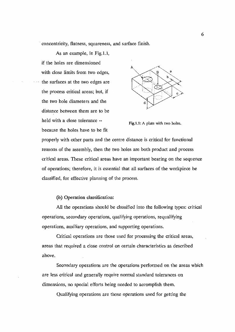
As an example, in Fig.Ll,

if the holes are dimensioned

with close limits from two edges,

the surfaces at the two edges are

the process critical areas; but, if

the two hole diameters and the

distance between them are to be

held with a close tolerance ~~

because the holes have to be fit

FJg..l.l: A plate with two holes.

6

properly with other parts and the centre distance is critical for functional

reasons of the assembly, then the two holes are both product and process

critical areas. These critical areas have an important bearing on the sequence

of operations; therefore, it is essential that all surfaces of the workpiece be

classified, for effective planning of the process.

(b) Operation classification:

All the operations should be classified into the following types: critical

operations, secondary operations, qualifying operations, requalifying

operations, auxiliary operations, and supporting operations.

Critical operations are those used for processing the critical areas,

areas that required a close control on certain characteristics as described

above.

Secondary operations are the operations performed on the areas which

are less critical and generally require normal standard tolerances on

dimensions, no special efforts being needed to accomplish them.

Qualifying operations are those operations used for getting the

. workpiece out of a rough condition. These are the first operations to

establish a newly machined surface for locating a workpiece.

7

Requalifying operations are the operations that are required to re­

establish a locating surface; this usually occurs when the part has experienced

any physical change during the machining processes or heat-treatment: such

as, distortion from stress relief, or surface damage due to clamping.

Auxiliary operations are those operations which change the physical

characteristics or appearance of the workpiece. Examples of operations in

this category include welding, heat treatment, finishing, and cleaning.

Supporting operations are the operations required to complete the

product successfully. These operations can not exist by themselves.

Operations such as shipping, receiving, inspection and quality control,

handling, and packaging fall into this category.

The general rules regarding the sequence of critical and secondary

operations are:

• In order to reduce the tolerance stacks, the critical operations that

establish the baseline dimensioning should be performed as early as

possible in the sequence.

" The critical operations, on the areas which require close tolerance

control, should be accomplished as early as possible in the sequence.

This is because the surfaces may be used as the locating surfaces for

other machining or gauging operations, Another reason is to save the

operation costs: if the part is likely to be scrapped, it should be

allowed to happen as early as possible.

• The critical operations that relate to the product critical areas should

be carried out as late as possible in the processing sequence. The

reason for this is to avoid any surface damage that may occur in the

later steps of manufacture.

For other classes of operations, their order of placement in the

sequence are largely governed by the critical operations.

( c) Principles of workpiece control:

8

From the above discussion, the process critical areas are to be

machined before other less important areas in the processing sequence.

However, on a workpiece there are usually several such areas; thus, a

procedure is required to determine the priority to be assigned to each area to

be machined. The priority assigned depends upon the amount of workpiece

control that each area can offer. Three types of workpiece control must be

considered are:

.. Geometric control: Geometric control relates to the stability of the

workpiece due to the geometric disposition of locators; for example,

the surface on which the locators can be placed wider apart gives a

better geometric control.

.. Mechanical control: Mechanical control relates. to the resistance to

movement of the workpiece under the cutting forces. The degree of

this control is reflected by the amount of workpiece deflection under

the cutting and holding forces.

.. Dimensional control: Dimensional control relates a direct effect on

the dimensional tolerances achievable on the machined part, which,

eventually, are the quality characteristics of the product. Therefore, it

is the most important control of all the three. Good dimensional

control is characterized by no tolerance stacks, and is achieved by

placing the locators on appropriate surfaces.

(d) Concept of workpiece locating:

A dimensions of a machined part is, in fact, the distance between the

surface of a locator and the cutting edge of a tooL So, to ensure the

uniformity in dimensions, every workpiece must be placed, as far as possible,

in the same position while being machined.

9

The concept of workpiece locating here is concerned only with the use

of locators to constrain the workpiece in a required position; it has nothing to

do with the holding forces. The general concept of locating can be stated as:

to locate an object in any position is to deprive the object of its six degrees of

freedom three translations and three rotations (Fig.1.2).

When the workpiece is

constrained by locators, like the

ones in Fig. 1.3, all the degrees

of freedom are stopped by the

six locators. This arrangement

of locators is known as the 3-2-1

location system, in which three

locating surfaces on the

workpiece must be mutually

FJ.g.l2: Six-degree of freedom.

nonparallel, (preferably) perpendicular planes. On some workpieces, these

locating surfaces must be established if they do not exist. This may be

achieved by incorporated them in the design of the part, and they may be

machined out in a later step of machining, or they may be left on the finished

part.

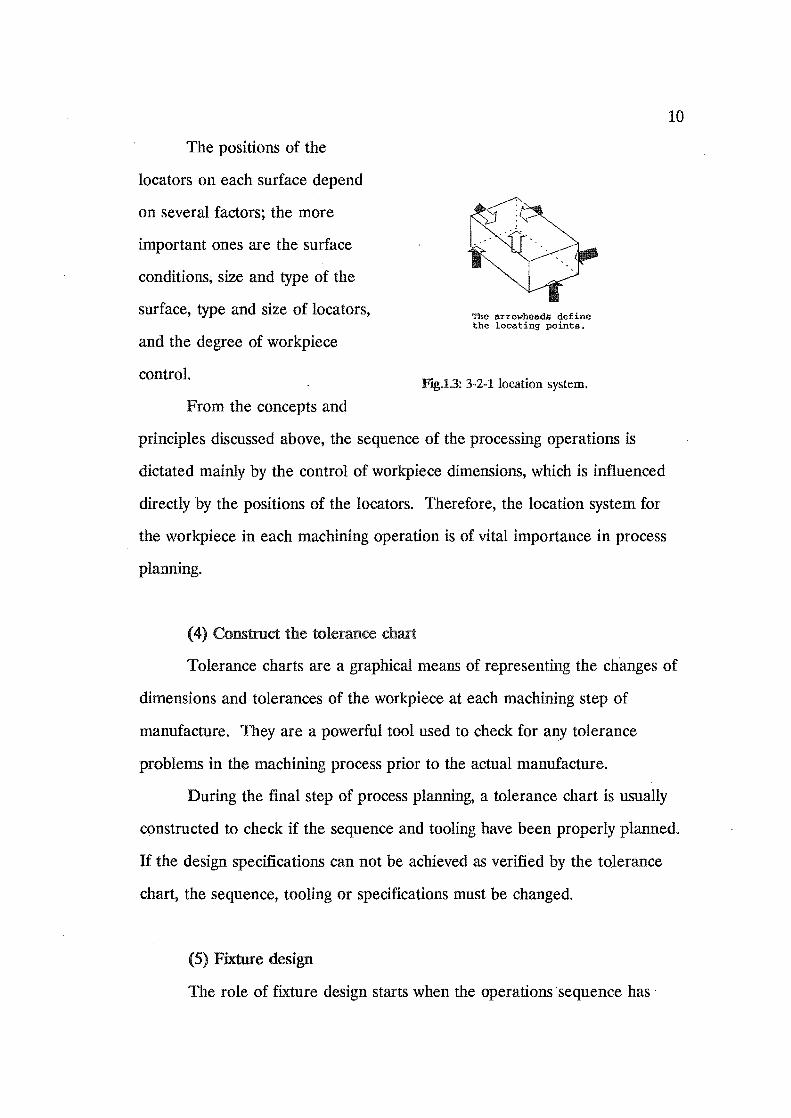
The positions of the

locators on each surface depend

on several factors; the more

important ones are the surface

conditions, size and type of the

surface, type and size of locators,

and the degree of workpiece

control.

From the concepts and

The arrowheads define the locating paints.

FIg.13: 3-2-1 location system.

principles discussed above, the sequence of the processing operations is

dictated mainly by the control of workpiece dimensions, which is influenced

directly by the positions of the locators. Therefore, the location system for

the workpiece in each machining operation is of vital importance in process

planning.

(4) Construct tolerance chart

10

Tolerance charts are a graphical means of representing the changes of

dimensions and tolerances of the workpiece at each machining step of

manufacture. They are a powerful tool used to check for any tolerance

problems in the machining process prior to the actual manufacture.

During the final step of process planning, a tolerance chart is usually

constructed to check if the sequence and tooling have been properly planned.

If the design specifications can not be .achieved as verified by the tolerance

chart, the sequence, tooling or specifications must be changed.

(5) Fixture design

The role of fixture design starts when the operations 'sequence has'

11

. been completed [9]. Traditionally, the task of tool designer includes: studying

the drawings of the part and the stock material; defining the positions for

locating, supporting and clamping the workpiece; and designing the fixturing

elements. However, if the fixture design is viewed as an integral part of

process planning, these pieces of information have already been established

when the operation sequence was planned. The tool designer can obtain this

information from the process engineer and use it directly in the designing of

the fixture. There is no need to replicate the task at the level of tool . .

designer. The main concern of the tool designer is to design the fixturing

elements, or choose them from available standard elements, and to make sure

that all the requirements entailing the workpiece and cutting tool are

functionally and economically achievable.

1.2 Literature review

It has been generally accepted for some time that process planning is

an important link to bridge the gap between design and production. In the

present advanced environments of Computer Aided Design (CAD) and

Computer-Aided Manufacturing (CAM), Computer Aided Process Planning

(CAPP) is an important key to the success of fully computerised

manufacturing, which is often referred to as CIM (Computer Integrated

Manufacturing).

There are two basic approaches to computerised process planning: the

variant approach and the generative approach. Variant process planning is

based on a predefined processing sequences for families of parts, these being

stored in a suitable form of database in the computer. This type of process

planning system usually requires a coding system for identifying the part

family, and therefore it is closely associated with the use of Group

12

Technology techniques [14]. To plan the processing sequence for a new part,

the characteristics of the part are coded; the code is then used to retrieve the

processing sequence from the database. The advantage of these variant

systems is that they are easy to develop and implement, and suitable for a

large number of different parts that can be grouped into a small number of

families. The main weak points of the systems are that they still require

human intervention during the planning stage; this may be necessary even if

there is only a slight difference in the design of the part being planned from

those whose sequences are already stored in the database. Typical variant

process planning systems areMIPLAN [15], CAPP-CAM-I [16], GENPLAN

[17], and Micro-CAPP [18].

The generative process planning system embodies the manufacturing

logic and uses it to generate the processing sequence for a part. The

limitation of the system depends only on the logic stored. Because this

manufacturing logic is compiled from experiences (know-how of the process

planners) and from other relevant scientific knowledge, this type of process

planning system is more difficult to develop than the previous one.

Nevertheless, the system can offer fully automatic planning without human

intervention. This makes the development of the system more challenging.

Since Wysk proposed the idea of automatic generative process planning in

1977, the approach has become widely researched in both industry and

universities. Examples of this type of process planning system include TIPPS

[19], CMPP [20], and AUTOPLAN [21].

There are also the systems that make use of both approaches. In these

systems, both variant and generative properties are built into a single system.

For example, ICAPP, which developed by Eskicioglu and Davies [22], is

capable of selecting the machining sequence for a part from each of a number

of families of parts stored in the system; and, to some extent, it can also

generate the plan according to the logic defined by the system.

13

Up to about the beginning of the 1980s, many research groups realised

the difficulties in encapsulating manufacturing logic using the conventional

programming methods. During the same period of time, Artificial

Intelligence (AI) research has produced some successful results in areas such

as medicine, chemistry, oil-field exploration, and computer configurations.

These and many other successful systems based on AI techniques have

inspired manufacturing researchers to launch the research using AI

techniques. By the middle of the 1980s, several AI based systems for process

planning had been developed. The systems incorporating AI techniques are

known as rule-based, or expert process planning systems. The attractive

characteristic of the expert system is that the manufacturing logic of the

expert is stored in the form of rules and these rules can be interpreted and

used to infer appropriate decisions. Examples of AI based CAPP systems

include GARI [23] and [24] for machining rotational parts, and the

system developed by Iwata and his research group in Japan [24], EXPLANE

[25], and HutCAPP reported by Mantyla [27] in Sweden for prismatic parts.

Although AI seems to be a promising technique for process planning (in

which its application is growing rapidly) there are some basic problems in

developing an expert system: firstly, there must exist an expert in the problem

domain of interest; secondly, the appropriate means must be available for

knowledge acquisition; and thirdly, it requires time. These problems make

the real practical expert system difficult to develop [28].

In developing a CAPP system, the method for representing the part in

the computer is also of vital importance. The requirement is that the method

used should be able -to provide both the geometric and the manufacturing

14

. information of the part. This has drawn other areas of research: such as,

solid modelling, feature recognition, and design by features, into the province

of CAPP research. The systems that reflect this multi-disciplinary knowledge

are, for examples, the expert system developed by Willis et al [29],

EXPLANE [26], STOPP [30], and FORM (Feature Oriented Modelling) [32].

Alting and Zhang[32] have made a comprehensive literature survey of

the state-of-the-art of CAPP systems, which has covered more than 200

published papers from all over the world, and more than 150 CAPP systems

have been included. Interestingly, most of CAPPs developed so far have not

adequately addressed the problem of dimensional control on the workpiece.

The research works in this direction are still few. Even though some attempts

[33,34] have been made to analyse dimensions of the part by means of

computers, the systems developed are not related directly to process planning.

Other CAPP researchers such as Weill [35], Sack[20], Chang, Wysk [36], and

Davies [37] have realised this problem, but so far no studies have been

reported that base process sequencing on dimensions and tolerances of the

part.

On the fixture design side, the research may be classified into 3 broad

categories: (1) the development of new methods of fixturing, (2) computerised

conventional fixture design, and (3) computerised modular fixture design. In

the first category, the research is directed at finding new methods for holding

workpieces. An example of this kind of research is the fluidized bed fixture

developed by Gandhi and Thompson [38]. The work that belongs to the

second category is concerned with the design, selection and assembling of the

conventional jig or fixturing elements such as locating pins, buttons, screw

clamps, strap clamps, etc. Examples of work in this category are: the

15

, 'Programmable Comformable Clamps' developed by Cutkosky et al [39] for

clamping turbine blade; the computer package for designing jigs and fixtures

for a Flexible Manufacturing System (FMS) developed by Drake [40]; and the

work reported by Berry [41] on the implementation of CAD/CAM to fixture

design. Other research contributions, based on an AI approach, that fall into

this category, include the work of; Miller and Hannam [42], Nee et al [43],

Anglert and Wright [44], Lim and Knight [45], Pham et al [46], Pham and

Lazaro [47], and Darvishi and Gill [48]. The third category is concerned with

the design of modular fixtures; the outstanding work which could be

considered as the prototype of AFD was developed by Markus et al [49] in

Hungary. In this computer package, an AI technique was implemented

through the use of Prolog. The program can generate automatically the

towers and supports to suit the identified points for locators and other

fixturing elements. This work started a new area of computer application,

and it inspired manufacturing researchers, including those mentioned above,

to turn to this research direction. Also included in this category are the

modular fixturing system of Woodward and Graham [50], the design

methodology based on the technique proposed by Gandhi and Thompson

[51], and Ngoi's system [52] for assembling of modular fixturing elements.

There is other research work which is not bound by any of the above

categories, because it is concerned with some special aspects of fixture design.

The work along this line includes that contributed by Chou et al [53] on the

application of the classic screw theory to identify the locating and clamping

points, by Lee and Haynes [54] on finite-element analysis of flexible fixturing

system, and by Halevi and WeiU[55] on the application of tolerance analysis

to fixturing design.

Trappy and Liu [56] have recently published a literature review on the

16

. computerised design of fixture; the conclusion is at present the fully

automatic fixture design has not been completely developed. Furthermore, in

order to realise such system, a theoretical base for analysing the general and

basic principles of the workpiece-fixturing relationship needs to be developed.

1.3 Problems in developing CAPP and AID systems

The problems encountered by researchers working on CAPP and AFD

can be listed as follows:

(a) Form of computer input:

Most of the systems developed so far depend on extensive

interaction between user and computer. That means the description of

the features on a part component must be first manually extracted

from the design, and then input in to the computer. This inefficient

method has led to the use of solid models to represent the part

geometry in the computer. Although much progress in solid modelling

technology has been made in recent years, further development is

required before it can be fully utilised in process planning [57].

(b) Extraction of features from a CAD system:

This problem is related to the first one. Because a solid model

does not provide the data that can be used by a CAPP system directly,

a means has to be devised to extract the required information from the

CAD database and store it in a usable form [58]. Research in this

area is still in an early stage but together with solid modelling it forms

the realm of feature recognition.

(c) The manufacturing information on a solid model:

A solid model of a part can only represent the geometrical

17

shape of the part. In process planning, not only the features on the

model must be extracted from the part model, but also the information

about manufacturing specifications must be supplied by some other

means to the system. This has led to the idea of attaching

manufacturing information to the features at the design stage; the

design representation of this nature is usually referred to as 'design by

features', or 'design with features'. However such a design

representation has not yet been adequately developed for machined

part designs; although, substantial progress has been made in relation

to casting designs in the United States [60].

(d) Tolerance control:

Although tolerance control is a basic issue in metal machining,

most of the CAPP systems do not take it into account. This is

probably because the recent advancement in machine-tool technology

has made available machine-tools capable of producing dimensions

with a far closer tolerance than in the past. This suggests that the use

of advanced machine-tools overcomes the problems of tolerance

stacking. But this is only true when only one setup is required for

machining the whole workpiece. In practice, a workpiece often

requires different setups for different operations and hence tolerance

control remains a basic issue.

Trappy, Liu [56] Alting and Zhang [32], all realise that this

aspect of control has been omitted from most of the research on both

CAPP and AFD.

1.4 Objectives and scope of the project

Although CAPP systems have been researched for more than 20 years,

. the results are still short of the requirements of industry [32]. One of the

obstacles is that the basic practical principles of process planning have been

mostly abandoned in the existing CAPP systems. Although AI is used, it is

used mainly for supporting the system, eg, for recognising a machining

18

. feature, rather than encapsulate the manufacturing knowledge. In those AI­

based systems that do incorporate the manufacturing knowledge, the

knowledge has been in the form of technical information extracted mainly

from books and publications which neglect the basic technological principles

completely.

The work reported here is, therefore, directed at demonstrating the

important role dimensional relationships between machined features have in

process planning and fixture design.

The general objective of the research is to investigate the feasibility of

using the principles of workpiece control as a guide to generating the

machining sequence. The thesis of this research is that automatic planning of

machining sequences can be achieved by applying practical basic principles.

In order to demonstrate the idea, a CAPP system with the following

characteristics was to be developed:

(1) The system is for prismatic parts with only three types of

machining features, namely; step, slot, and plane surface.

(2) The machining operations are confined to milling.

(3) The system is capable of creating the machining sequence

automatically.

(4) The system is equipped with a tolerance control technique: the

tolerance chart.

(5) In connection with fixture design, the system is able to provide

the fixture designers with information such as the appropriate

19

locating surfaces (in 3-2-1 location system) on the workpiece for

each machining operation. It is not intended to consider the

design of the fixture body.

(6) In addition to the above characteristics, the system is

implemented on a Pc.

Progrmming technique

While the sequencing facilities in most existing CAPP systems are

based on the changes of the workpiece geometry alone, the system developed

here uses the two types of workpiece control: dimensional and geometric, as a

basis for planning the sequence of machining.

Although at present the expert system approach has been widely

adopted in CAPP systems, the real expert system for process planning has not

yet been realised. It will appear that the best method of developing an expert

system requires the actual expert in a particular problem domain to undertake

the development himself. This requires time for him to study the principles

and logical concepts of expert systems. Even so after an expert system has

been developed, it still requires a real expert to test, modify and maintain the

system. These are the obstacles to a successful expert system in this area of

research. On the other hand, a system based on the conventional

programming technique, whilst it does not provide the same level of flexibility

as an expert system, requires less time to develop and hence is suitable for

testing the feasibility of an approach to a problem which requires a

procedural steps for solution. The results of this could help reduce the work

of a real expert in developing an expert system, because the expert system can

be confined to the narrower area which requires the practical skill and

experience.

20

Because mechanical control is more concerned with the experience. of

a tool designer in designing or choosing fixturing elements, this aspect of

workpiece control is more suitable for an expert system than is dimensional

and geometric control. This project, which demonstrates the implementation

of the latter, therefore uses the conventional programming technique.

1.6 Computer-aided process planning and fixture design system

(CAPPFD)

Since there is no intention to research in areas relating to solid

modelling, a simple part model representation has been adopted in the system

developed. This representation limits the capability of the system to prismatic

parts having edges parallel to x-, y-, or z-axis, and to two-dimensional

machined features. The system is capable of generating the machining

sequence for three types of machined feature, namely, plane surfaces, steps

and slots.

In executing the program, CAPPFD starts from reading the part model

data from a data file, executing the input routine for other data, sequencing

the machining operations, designing the location systems, and finally drawing

the tolerance charts for all process dimensions.

1.7 Conclusion

Process planning and fixture design are closely inter-related. A

processing sequence can not be planned properly without considering the

location systems; likewise, an economic fixture design can only be designed

when the machining sequence is available. The objective of this research

project is to demonstrate how this desirable point can be achieved by making

use of the dimensional relationships from the finished part drawings.

21

. 2. TOLERANCE CHART TECHNIQUE

Since· the aim of process planning is to achieve the design

specifications, it is essential that the process plan be checked for its

practicality: in this respect a tolerance chart is an indispensable tool.

However, the manual procedures available for tolerance charting are not

appropriate for computer programming, therefore a new method of tolerance

charting was developed during the course of this research. The method

developed not only facilitates the computerised charting, but also helps

reduce time and errors in manual charting. This chapter introduces the

background of the tolerance chart, and then details the development of the

new charting technique.

Tolerance charts

A tolerance chart is a graphical representation of a machining

sequence on a part. It shows dimensions and tolerances for the machining

cuts and for the stock to be removed at all steps of manufacture. It is an

analysis tool used by the process planner for assessing the feasibility of a

machining sequence prior to the actual machining operations. It is also a .

means of communication between the process engineers and product

designers. The comprehensive summaries of its uses are listed in Ref [12, 61,

62]. Other specific uses of the tolerance chart include:

(a) By coordinating with quality control charts, it can be used to

define the relationship between dimensional analysis and

dimensional control [63].

1 .2 3 4 5 6

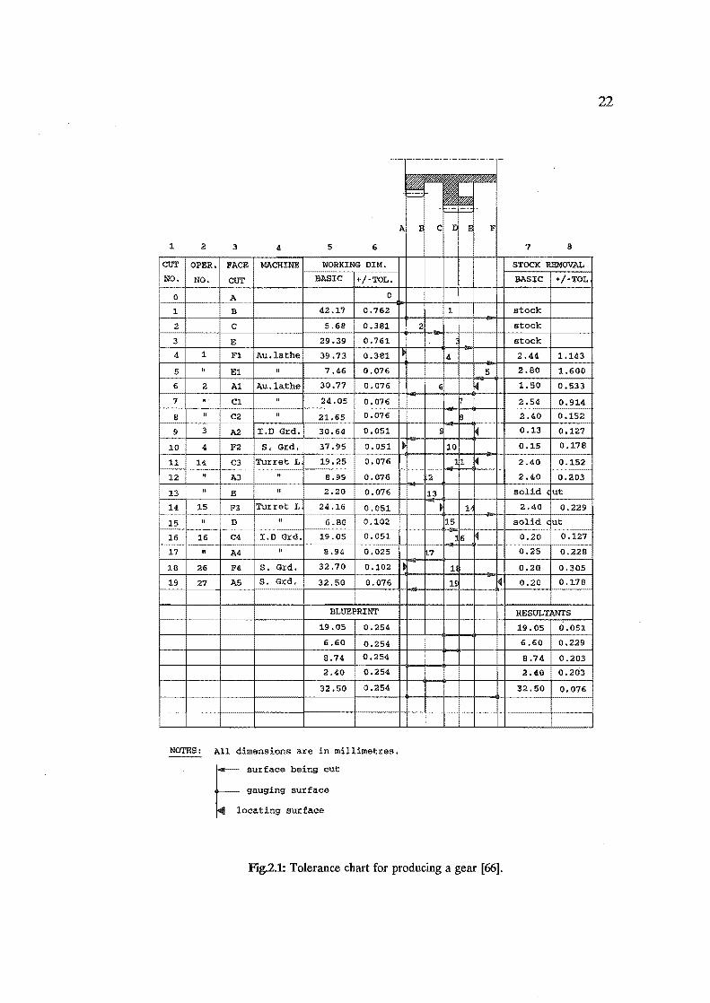
NOTES: All dimensions are in rnillirnet%8s.

f, surface being cut

gauging sU%face

locating surface

FJg2.1: Tolerance chart for producing a gear [66].

22

7 8

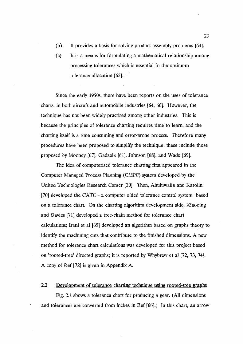
23

(b) It provides a basis for solving product assembly problems [64].

(c) It is a means for formulating a mathematical relationship among

processing tolerances which is essential in the optimum

tolerance allocation [65].

Since the early 1950s, there have been reports on the uses of tolerance

charts, in both aircraft and automobile industries [64, 66]. However, the

technique has not been widely practised among other industries. This is

because the principles of tolerance charting requires time to learn, and the

charting itself is a time consuming and error-prone process. Therefore many

procedures have been proposed to simplify the technique; these include those

proposed by Mooney [67], Gadzala [61], Johnson [68], and Wade [69].

The idea of computerised tolerance charting first appeared in the

Computer Managed Process Planning (CMPP) system developed by the

United Technologies Research Center [20]. Then, Ahuluwalia and Karolin

[70] developed the CATC - a computer aided tolerance control system based

on a tolerance chart. On the charting algorithm development side, Xiaoqing

and Davies [71] developed a tree-chain method for tolerance chart

calculations; Irani et al [65] developed an algorithm based on graphs theory to

identify the machining cuts that contribute to the finished dimensions. A new

method for tolerance chart calculations was developed for this project based

on 'rooted-tree' directed graphs; it is reported by Wbybrew et al [72, 73, 74].

A copy of Ref [72] is given in Appendix A.

2.2 Development of tolerance charting technique using rooted-tree graphs

Fig. 2.1 shows a tolerance chart for producing a gear. (All dimensions

and tolerances are converted from inches in Ref [66].) In this chart, an arrow

24

. points to the surface being machined, and a dot denotes a locating surface or

the surface from which the dimension of the corresponding cut is measured.

From now on, a surface identified by this dot is simply called a locating

surface (or a locating face). From each vertical face on the part sketch there

. is a line drawn downwards throughout the length of the chart; this line

represents a surface and is labelled with a capital letter. There are columns

for: the basic dimensions resulting from the machining cuts, which are

normally cal~ed 'working dimensions'; the machining tolerances; the stock

removal dimensions; the tolerances on stock removal dimensions; the drawing

dimensions and tolerances; and the resultant dimensions and tolerances.

Other columns are used for recording types of machine, operation numbers,

and letters identifying the surfaces reSUlting from the cuts. Some other

tolerance charts provide an extra column for balance dimensions: the

dimensions which are the results of two or more cuts. However, the balance

dimensions are not shown in this chart; the reason for this will be clear when

the technique has been fully explained. All the tolerances are expressed in

the equally bilateral system. Because the tolerance chart is concerned mainly

with the tolerances on length dimensions, the details of diametral or traversed

dimensions are omitted from this analysis. It should be noted that the stock

dimensions are also included in the chart as the working dimensions.

To construct a tolerance chart for a machined part, first the basic

information is filled in the prepared chart form. This basic information

includes the drawing specifications of the part, the sequence of machining, the

processing tolerance and the amount of stock removal at each cut, and the

type of machine for each operation. After this the calculations are made to

find the working dimensions and tolerance stacks on the stock removals and

on the resultant dimensions.

25

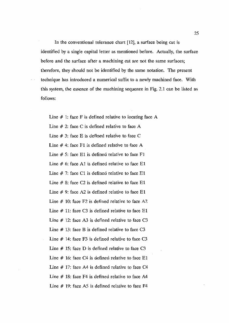
In the conventional tolerance chart [12], a surface being cut is

identified by a single capital letter as mentioned before. Actually, the surface

before and the surface after a machining cut are not the same surfaces;

therefore, they should not be identified by the same notation. The present

technique has introduced a numerical suffix to a newly machined face. With

this system, the essence of the machining sequence in Fig. 2.1 can be listed as

follows:

Line # 1: face F is defined relative to locating face A

Line # 2: face C is defined relative to face A

Line # 3: face E is defined relative to face C

Line # 4: face Fl is defined relative to face A

Line # 5: face El is defined relative to face Fl

Line # 6: face Al is defined relative to face El

Line # 7: face Cl is defined relative to face El

Line # 8: face C2 is defined relative to face

Line # 9: face A2 is defined relative to face El

Line # 10: face F2 is defined relative to face A2

Line # 11: face C3 is defined relative to face El

Line # 12: face A3 is defined relative to face C3

Line # 13: face B is defined relative to face C3

Line # 14: face F3 is defined relative to face C3

Line # 15: face D is defined relative to face C3

Line # 16: face C4 is defined relative to face El

Line # 17: face A4 is defined relative to face C4

Line # 18: face F4 is defined relative to face A4

Line # 19: face AS is defined relative to face F4

26

This can be summarized diagrammatically in the rooted-tree graph as

shown in Fig. 2.2 where each node represents a locating surface or a

machined surface or both, and an arrow points to a machined surface. The

working dimension is represented in this diagram as a link between two

nodes, and identified by a line number (or a cut number).

Fl

Aq<iII-_9_( 0_, o_5_...:.1)--1,

10 (0, 1)

F3

A3

FJg.2.2: The rooted-tree diagram for producing a gear.

In this graph, the path from anyone node to another defines the cuts

that contribute to the distance -- dimension and tolerance -- between the two

surfaces denoted by the nodes. For example, the resultant dimension

between B and C4 is the result of cuts 11, 13, and 16; and its tolerance is the

sum of these machining tolerances. Or, the tolerance stack on stock removal

27

. at cut 7 is the sum of the tolerances of the links in the path from node Cl to

node C. Therefore, by using the rooted-tree diagram, the cuts that give rise

to any pair of surfaces can be readily identified.

The rooted-tree graph method provides a convenient means to

calculate the tolerance stacks, on either the stock removal dimensions, or on

the resultants; it can also be used to calculate the working dimensions in most

practical cases as explained in Ref [72, 73]. However, in some uncommon

cases where locating surfaces for machining a surface are changed often in

the course of machining, the technique is not able to derive some working

dimensions. Therefore a study was made on the fundamental aspects of the

working dimensions. It was found that any working dimension is the result of

adding or subtracting the drawing dimension with the stock removal

dimension(s). This is the basic procedure in manual charting, and it is

adopted here.

2.3 A method for calculating working dimensions

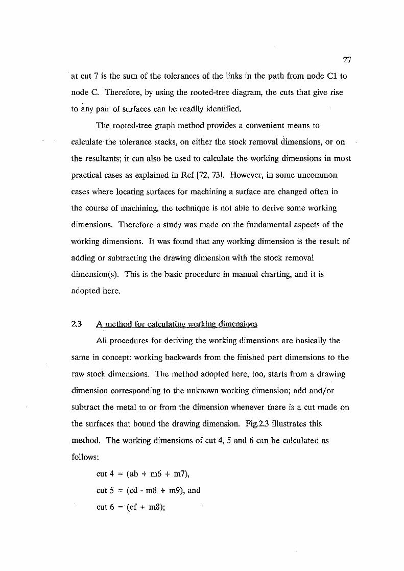
All procedures for deriving the working dimensions are basically the

same in concept: working backwards from the finished part dimensions to the

raw stock dimensions. The method adopted here, too, starts from a drawing

dimension corresponding to the unknown working dimension; add and/or

subtract the metal to or from the dimension whenever there is a cut made on

the surfaces that bound the drawing dimension. Fig.2.3 illustrates this

method. The working dimensions of cut 4, 5 and 6 can be calculated as

follows:

cut 4 (ab + m6 + m7),

cut 5 = (cd - m8 + m9), and

cut 6 =' (ef + m8);

m

m9

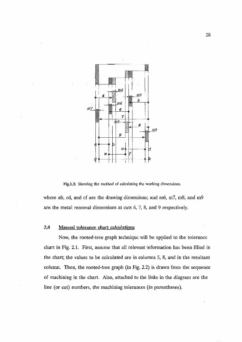
Ftg.13: Showing the method of calculating the working dimensions.

where ab, cd, and ef are the drawing dimensions; and m6, m7, m8, and m9

are the metal removal dimensions at cuts 6, 7, 8, and 9 respectively.

2.4 Manual tolerance chart calculations

28

Now, the rooted-tree graph technique will be applied to the tolerance

chart in Fig. 2.1. First, assume that all relevant information has been filled in

the chart; the values to be calculated are in columns 5, 8, and in the resultant

column. Then, the rooted-tree graph (in Fig. 2.2) is drawn from the sequence

of machining in the chart. Also, attached to the links in the diagram are the

line (or cut) numbers, the machining tolerances (in parentheses).

29

(a) Calculations of tolerance stacks:

As mentioned earlier, the tolerance stacks on the stock removal and on

the resultant dimensions are calculated by summing up the machining

tolerances of the links in the relevant paths. Therefore, to calculate the

tolerance stack on the stock· removal at cut 6, first, from the graph, pick up

the path with the starting node Al and the ending node A, or vice versa;

then, sum up the tolerances on the links:

0.076 + 0.076 + 0.381 0.533 mm.

Note that Al and A are the surfaces that bound the stock removal

dimension at cut 6, and the numerical suffixes of the two surfaces are

different by 1.

The same procedure is applied to the tolerance stacks on the resultant

dimensions. The only difference is the starting and ending nodes are defined

by the drawing dimensions instead of the stock removal dimensions. For

example, the tolerance stack on the drawing dimension between surfaces C4

and is equal to the sum of tolerances on cuts 16, 11, and 15:

0.051 + 0.076 + 0.102 == 0.229 mm.

Surfaces C4 and. D are both the last machined surfaces which give the

drawing dimensions. In Fig.2.2, all the last machined nodes are surrounded

by two circles to make them different from the others so that they can be

identified easily.

30

(b) Calculations of working dimensions:

To calculate the working dimensions, consider the tolerance chart in

Fig.2.1, trace up along the two surfaces from the drawing dimension

corresponds to the working dimension in question, and add or subtract, as the

case may be, the drawing dimension with the amount of stock removal at

each cut that encounters the surfaces. The conditions to add or subtract the

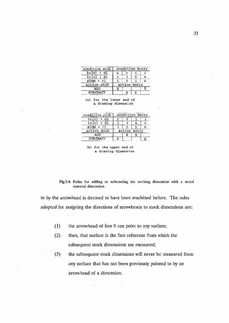
working dimension with the stock removal can be summarized in two decision

tables, shown in Fig.2.4. (A brief discussion of decision tables is given in

Appendix E.) In this figure, d1 and d2 are the lower and the upper ends of a

drawing dimension; lo[ c] is the locating surface for a cut, which is made on

the surface below the unknown working dimension; and 'SIGN' is a variable

identifying if a particular cut shortens or lengthens the distance between two

surfaces. If a cut results in a shorter distance -- that is the distance between

two surfaces after the cut is shorter than before the cut, SIGN is ~1;

otherwise, + 1. With the rules in the tables, the working dimensions of cuts 2,

and 3 can be calculated as follows:

cut 2:

8.74 - 0.20 - 2.40 - 2.40 - 2.54 + 0.20 + 0.25 + 2.40 + 0.13 + 1.50 =

5.68 mm.

cut 3:

19.05 + 2.80 + 0.20 + 2.4 + 2.4 + 2.54 = mm.

(c) Notes on stock dimensions, tolerances and solid

If a machined part is machined from a casting or stock with specific

sizes, its dimensions are included at the top part of the chart. Since these

dimensions have to be treated like working dimensions, an arrowhead and a

. dot are required for each of them. Each of the dimensioned surface pointed

condition stub condition entry 10 [cl > dl 0 0 1 10 [c] < d1 1 1 n SIGN m +1 1 0 1

;;,...j-~ '" ADD X I

SUBTRACT X X -

(a) for the lower end of a drawing dimension

1 n 0

:x:

condition stub conditlon entry 10 [c] > d2 0 0 1 10 [c] < d2 1 1 n SIGN = +1 1 0 1

action stub action entry ADD X

SUBTRACT X

(b) for the upper end of a drawing dimension

X

1 n ._ .. -0

X

31

FJg.2.4: Rules for adding or subtracting the working dimension with a metal removal dimension.

to by the arrowhead is deemed to have been machined before. The rules

adopted for assigning the directions of arrowheads to stock dimensions are:

(1) the arrowhead of line 0 can point to any surface;

(2) then, that surface is the first reference from which the

subsequent stock dimensions are measured;

(3) the subsequent stock dimensions will never be measured from

any surface that has not been previously pointed to by an

arrowhead of a dimension.

32

ABC D E ABC D E ABC D E

I~ ~

o ~ ~

f---<

o !4 J Z

~ >----+

~

(a) stock dimensions (b) working dimensions (c) working dimensions

Ylg.25: The method for converting the stock dimensions to the working dimensions.

Fig.2.5 shows two examples of converting stock dimensions to working

dimensions. The stock dimensions are given in (a). If the arrowhead of line

o is assigned to surface D, then the stock dimensions can be represented as in

(b); but, if surface A is chosen to be the starting surface, then the result is ( c).

Note that the changes in positions of the working dimensions depend on the

surface chosen for line O.

In a tolerance chart, the word 'solid' is inserted to the first cut made

on a surface in the column of stock removal dimensions. This is a normal

practice when the part is machined from a bar stock, and no stock dimension

is given. This practice still applies to the case where stock dimensions are

treated as working dimensions; but the word such as 'stock' or 'casting' or

'forging' is.used instead of 'solid', And the machining tolerances of these

working dimensions are the tolerances on the stock dimensions.

2.5 Computer program for tolerance charting

Fig.2.6 shows the macro-flow chart of the computer program for

tolerance charting. This program is then combined with the program for

. sequencing the machining operations and locating the workpiece, which will

be explained in the subsequent chapters, to become a fully computerised

process planning and fixture design program.

33

In box 1, the distances between surfaces(A, B, C, etc) are calculated

from drawing dimensions and stored ina 2D-array. This distance matrix

facilitates the calculations of working and resultant dimensions. In box 2 all

working dimensions are calculated. Before a tolerance stack on a stock

removal dimension can be calculated, a path containing the cut numbers is

created between the two faces of the metal removal, and then the tolerance

stack is calculated. This is shown in boxes 3 and 4. The same procedure is

also applied to calculate both the tolerances (boxes 5 and 6) and the

dimensions of the resultants (boxes 7 and 8). These resultant dimensions can,

in fact, be copied directly from the drawing dimensions; however, in this

program, as a check, they are calculated back from the known working

dimensions. In box 9 the results are printed.

Note that the program does not store all the paths from the cut faces

to the root; it creates the path when required; after the path has been used

the memory of it is not retained.

1. Create matrix

Calculate the working

·3. Create a path between the two cut faces of the stock removal

4. Calculate tolerance stack on stock removal

For all resultants

from the a drawing

, .... ~------,---------'

6. Calculate the tolerance stack on a resultant

c-.... For all resultants

Create a path from the' two ends of a drawing dimension

B. Calculate a resultant dimension

. 9. Print the results from the calculations

Fig.2.6: Macro flow-chart for tolerance chart calculations.

34

35

. 2.6 Conclusion

The details of tolerance charting with the new technique have been

explained. A computer program, based on this technique, was developed,

tested and found to work well with data from various publications [61-63, 66-

69, 75] (some of the test results are shown in Appendix C). When used in

manual charting, it was found that the technique could reduce the time

required, and the number of errors made. It could also be used as a

supplementary tool to other charting techniques such as Wade's and

Gadzala's methods. For a comparison, the reproduction of the latter is given

in Appendix D.

36

, 3. SYSTEM STRUCIURE

The Computer~Aided Process Planning and Fixture Design (CAPPFD)

system developed in this project is written in C and implemented on a PC,

with a base memory of 640 K bytes, under the DOS operating system. In this

chapter the overview of CAPPFD is presented. This includes the types and

general characteristics of the features that the system can handle, and the

program modules that constitute the system.

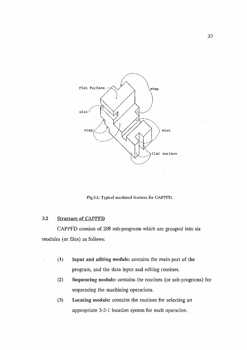
3.1 Machined features for CAPPFD

Although the system is designed to work on a prismatic part, which is a

three-dimensional object, the machined features on the part are confined to

two-dimensional ones. Here, the two-dimensional feature may be defined as

a machined feature comprised of only flat surfaces; each of them being

parallel to one of the principal planes. Therefore, the feature can be

presented graphically and dimensionally in two orthogonal projection views.

The common machined features that fall into this category are flat surfaces,

steps, and slots; examples of these are shown in Fig. 3.1. The features chosen

to work with are limited by the workpiece model representation inside the

computer (which will be described in the next chapter). But these features

are sufficiently general to form a basis to demonstrate the concept used for

computerized process planning and fixture design.

flat fur face step

slot

slot

Fig.3.1: Typical machined features for CAPPFD.

3.2 Structure of CAPPFD

CAPPFD consists of 208 sub-programs which are grouped into six

modules (or files) as follows:

(1) Input and editing module: contains the main part of the

program, and the data input and editing routines.

37

(2) Sequencing module: contains the routines (or sub-programs) for

sequencing the machining operations.

(3) Locating module: contains the routines for selecting an

appropriate 3-2-1 location system for each operation.

(4) Tolerance chart module: contains the routines for producing

tolerance charts.

(5) Support Module: contains the routiiles for the following two

main functions:

~ .. producing the drawings of the part on the screen or on the

printer, with or without the locating symbols; and

• extracting the coordinates of the surfaces on the part and

storing them in a set of linked lists.

38

(6) Utilities module: contains two sets of routines of which the first

contains the general purpose sub-programs that are used by

almost every module, ego the routines for allocating and freeing

the dynamic memories, and the second is concerned with

modifying the workpiece model representation and storing it in

a dummy data file.

Fig.3.2 shows the inter-relationships among the modules mentioned

above. The data files are also included here to complete the overall structure

of the system. These data are of two types: the first is the model

representation data, and the second is, the so called, 'production data' -- ego

depths of cuts, number of cuts, processing tolerances, etc.

3.3 CAPPFD flowchart

Fig.3.3 shows the simplified flowchart of the CAPPFD system. Also

included in the figure are types of data and program modules required at

various stages of execution; the data are in dotted line boxes, and the

program modules, in full line boxes.

The system starts with the input of data which consists of two steps: in

the first step, the input and editing module reads the part model

... U<..J .... Structure of the CAPPFD system.

representation data, which have already been stored in a data file; this is

followed by the second step: the input of the production data. Two options

are provided for inputting the production data: the user either interactively

inputs the data into the system, or let the system read the data from a data

file, which requires the data be previously stored in a data file.

39

After the data input session is completed, the sequencing module starts

to sequence the machining operations; this requires data such as drawing

tolerances, the surface numbers that constitute each feature, etc. The result

of this execution is the machining sequence.

Then, the locating module determines the 3-2-1 location system for

machining each feature. The same location system is used for all cuts that

are required to produce a particular feature .. During this stage of execution,

the system displays all the location systems on the monitor screen, and if

required, the outputs can also be printed out on a line printer.

Spatial representation of the part

. i:;;~~i'~g' 't~i~:r-~~~'~~:': surface numbers . constituting , each feature, etc. :

.......................... I

, , : Stock tolerances ;. ... ...,-_-'-_--1. ____ --, , , .......................

Production data: : .. ego depths of cuts,: "--___ -,-____ ...J

process tolerances :

Input and editing module

Sequencing module

Locating module

Tolerance chart module

FJg33: Macro-flowchart of the CAPPFD system.

40

In the final step, the system performs tolerance chart calculations and

draws the tolerance charts. Three tolerance charts are drawn on the screen.

The user can also print the screen outputs on the printer if required.

The user may modify the processing tolerances by re-running the

system and using the editing routines to modify the data. The sequence of

the operations resulting from the system cannot be modified. This is required

to preserve the merits of the system: the system tries to achieve the best

combination of dimensional control and geometric control. However,

modifications of the sequence could be made indirectly by altering design

dimensions or by modifying the values of design tolerances.

3.4 Conclusion

The CAPPFD system contains 6 program modules, namely; the input

and editing module, the sequencing module, the locating module, the

tolerance chart module, the support module, and the utilities module. It is

capable of sequencing three types of machined feature, ie, plane surfaces,

steps and slots.

41

This chapter serves as an introduction to the details that follow in the

subsequent chapters: chapter 4 discusses the data structures, and the input

and editing module; chapter 5 explains how the machining operations are

sequenced; chapter 6 discusses the details of the locating module and the

algorithm for modifying the workpiece model representation; chapter 7

describes how the tolerance chart program is integrated in the main package;

chapter 8 shows two examples of the implementation of the system, and

chapter 9 is the conclusion of this research project.

42

. 4. DATA; STORAGE, INPUT AND OUIPUT

CAPPFD stores all geometric data of a machined part in a three­

dimensional array, the amount of memory for which is allocated dynamically,

and depends on the complexity of the part. This simple technique for solid

modelling was developed by Ngoi [52]. However, the part model does not

incorporate other essential information such as the identification of surfaces

that bound a feature, the tolerances on dimensions, or the cutting conditions

required for each feature. This information is regarded roughly as the

'production data', and is stored separately. This chapter discusses the

structures and the input/output of CAPPFD data.

Although the part model is a 3D-array and any array operations can be

performed on it, some of the object elements of this array represent different

conditions from the others. This is the essence of the technique; it is

described in the following section.

4.1 Spatial representation technique

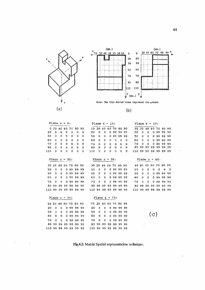
The spatial representation technique is a method for representing the

geometry of a part inside the computer which makes use of a series of two

dimensional arrays to define the part geometry. To illustrate the concept of

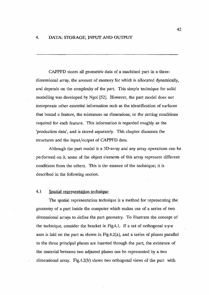
the technique, consider the bracket in Fig.4.1. If a set of orthogonal x-y-z

axes is laid on the part as shown in Fig.4.2(a), and a series of planes parallel

to the three principal planes are inserted through the part, the existence of

the material between two adjacent planes can be represented by a two

dimensional array. Fig.4.2(b) shows two orthogonal views of the part with

. horizontal and vertical planes at

various x, y and z coordinates.

The spatial representation of

the bracket along z-axis is

shown in FigA.2(c). The

numbers in the first row, except

the first one, denote the x­

coordinates; the numbers in the

first column, except the first

one, denote the y-coordinates.

43

90.0 110.0

F'tg.4.1: A bracket (in rom.)

The number in the first row and the first column of each array denotes the z­

coordinate. The other numbers, non-zero and zero numbers, denote

respectively the existence and non-existence of the material between one

plane and the next lower plane. Therefore, in the array at z=49.0, the zero

defined by row 1 and column 4, indicates that there is no material of the part

from x=70.0 to x=60.0, from y=20.0 to y=O.O, and from z 49.0 to z=39.0

mm; while the number 99 in the array at z =39.0 in row 1 and column 4

indicates the existence of the part material from x=70.0 to x=60.0, from

y=20.0 to y=O.O , and from z=39.0 to z=3S.0 mm .

. The decimal point numbers are used because all array elements are

required be of the same data type. However, in Fig.4.2 all decimal points are

omitted for clarity.

To input the spatial repr~sentation of a part into the computer, the

drawings of the part are first converted to a form as in FigA.2(b), from which

a series of two dimensional arrays of numbers can be readily constructed.

Then the numbers are arranged in a data file for the computer to read. At

present this procedure is done manually.

x

Plane z - 0:

o 20 40 60 70 80 90 20 0 0 0 0 0 0 50 0 0 0 0

60 0 0 0 0 70 0 0 0 0 80 0 0 0 0

110 0 0 0 0

Plane z = 35:

o 0

o 0 o 0 o 0 o 0

35 20 40 60 70 80 90 20 0 0 0 99 99 99 50 0 0 0 99 99 99 60 0 0 0 99 99 99

70 0 0 0 99 99 99 80 99 99 99 99 99 99

110 99 99 99 99 99 99

Plane z = 55:

55 20 40 60 70 80 90

20 0 0 0 99 99 99 50 0 0 0 99 99 99 60 0 0 0 99 99 99

70 0 0 0 99 99 99 80 99 99 99 99 99 99

110 99 99 99 99 99 99

z 75

(nun. ) (nun. )

39 35 3010 0 o 20 40 60 70 SO 90 x . . ., .,

w ...... ; •• 20 20 .. ~. ";" . I ••• ~.IU~.II'

· . · '., . 50 50 • , " ... 4 • ~ ". •• , •• ~ " •• · . . . , · , . . ,

70 70 . . ..................... , ..

. . ....... ~ . ~ ~ . · . · . . . , 80 .. 80 - ... -~~ ... ~.~~~ .... " .. 110 110

Y{nun.)Y

Note: The thin dotted lines represent the planes.

(b)

plane z = 10:

10 20 40 60 70 80 90 20 0 0 0 99 99 99 50 0 0 60 0 0 70 0 0 80 0 0

110 0 0

Plane z

o 99 99 99 o 0 0 0 o 0 0 0 o 0 0 0 o 000

39:

39 20 40 60 70 80 90 20 0 0 0 99 99 99 50 0 0 0 99 99 99 60 0 0 0 99 99 99

70 0 0 0 99 99 99 ao 99 99 99 99 99 99

110 99 99 99 99 99 99

Plane z ~ 75:

75 20 40 60 70 ao 90

20 0 0 0 99 99 99 50 0 0 0 99 99 99 60 0 0 0 99 99 99

70 0 0 0 99 99 99 80 99 99 99 99 99 99

110 99 99 99 99 99 99

Plane z = 30:

20 40 60 70 ao 90 20 0 0 0 99 99 99 50 0 0 0 99 99 99 60 0 0 0 99 99 99 70 0 0 0 99 99 99 80 99 99 99 99 99 99

110 99 99 99 99 99 99

Plane z = 49:

49 20 40 60 70 ao 90

20 0 0 0 0 0 0 50 0 0 0 99 99 99 60 0 0 0 99 99 99

70 0 0 0 99 99 99 80 99 99 99 99 99 99

110 99 99 99 99 99 99

( C)

Flg..42: Matrix Spatial representation technique.

44

45

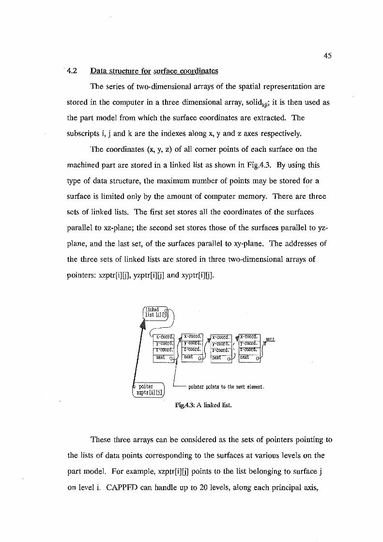
. 4.2 Data structure for surface coordinates

The series of two-dimensional arrays of the spatial representation are

stored in the computer in a three dimensional array, solidkji ; it is then used as

the part model from which the surface coordinates are extracted. The

subscripts i, j and k are the indexes along x, y and z axes respectively.

The coordinates (x, y, z) of all corner points of each surface on the

machined part are stored in a linked list as shown in FigA.3. By using this

type of data structure, the maximum number of points may be stored for a

surface is limited only by the amount of computer memory. There are three

sets of linked lists. The first set stores all the coordinates of the surfaces

parallel to xz-plane; the second set stores those of the surfaces parallel to yz­

plane, and the last set, of the surfaces parallel to xy-plane. The addresses of

the three sets of linked lists are stored in three two-dimensional arrays of

pointers: xzptr[iJU], yzptr[i]U] and xyptr[i]fj].

pointer points to the next element.

FJg.4.3: A linked list.

These three arrays can be considered as the sets of pointers pointing to

the lists of data points corresponding to the surfaces at various levels on the

part model. For example, xzptr[i]fj] points to the list belonging to surface j

on level i. CAPPFD can handle up to 20 levels, along each principal axis,

46

. with up to 5 surfaces on each leveL While extracting the surface coordinates,

the system also attaches to each surface an integer identifying the direction of

its normal out of the part: + 1 denotes a surface facing away from the origin,

and -1, facing towards the origin. This information is used in all stages of

execution -- sequencing, locating, and charting; it is stored in the following

arrays: xzd[i][j], yzd[i][j] and xyd[i][j], corresponding to the three sets of linked

lists mentioned above.

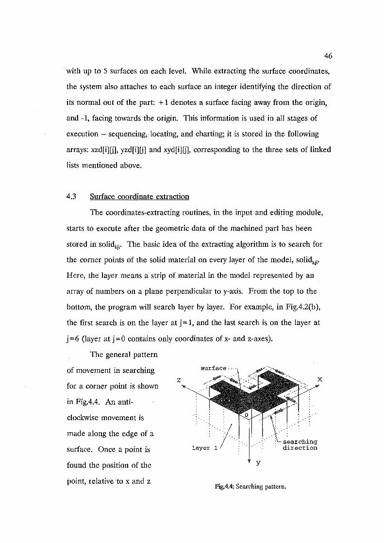
4.3 Surface coordinate extraction

The coordinates-extracting routines, in the input and editing module,

starts to execute after the geometric data of the machined part has been

stored in solidkji . The basic idea of the extracting algorithm is to search for

the corner points of the solid material on every layer of the model, solidkji•

Here, the layer means a strip of material in the model represented by an

array of numbers on a plane perpendicular to y-axis. From the top to the

bottom, the program will search layer by layer. For example, in Fig.4.2(b),

the first search is on the layer at j = 1, and the last search is on the layer at

j =6 (layer at j =0 contains only coordinates of x- and z-axes).

The general pattern

of movement in searching

for a corner point is shown

in Fig.4.4. An anti-

clockwise movement is

made along the edge of a

surface. Once a point is

found the position of the

point, relative 'to x and z

z

, ,

--:-"'y: : , '" , " , :. , ~ '. i ~ • . .. ~ ,

layer 1 ", "': :

y

. , ~. . ~.~

~~ ~ . ~ :

sea:rching direction

FJg.4.4: Searching pattern.

x

47

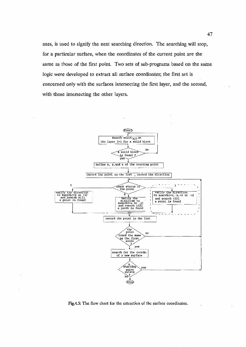
. axes, is used to signify the next searching direction. The searching will stop,

for a particular surface, when the coordinates of the current point are the

same as those of the first point. Two sets of sub-programs based on the saine

logic were developed to extract all surface coordinates; the first set is

concerned only with the surfaces intersecting the first layer, and the second,

with those intersecting the other layers.

1

tax

search solid kji on the layer j-l for a solid block

define x,

record the point in the list , record the direction

the point

found the same B the first

point ?

- :l ->---''------,

I ver1 yt'fie rect10n to search(+x, -x,+z or -z) i I

and search till a point is found

no

yes

FJg.45: The flow chart for the extraction of the surface coordinates.

48

Fig.4.5 shows the algorithm for extracting the surface coordinates of

surface intersections on the first layer. The program searches for a solid

block row by row, from row z= 1 to row z=7 in the model. If the first solid

block is found, the coordinates of the starting point of the block are

determined. These coordinates are then stored in the linked list; at the same

time, a number identifying the facing direction is assigned to the surface and

stored in the corresponding array. Mter the first point is found, its position is

then used as an index to signify the direction for the next search. This index , -

is defined in the flow chart as the status of a point which is identified by an

integer, from 1 to 3. Status 1 signifies that the current point found is on x­

axis, and there are only two possible directions: +x and + z, to search for the

next point. Likewise, status 2, the current point is on z-axis, and the possible

searching directions for the next point are +x and -z. The decision on which

direction to be chosen depends on the conditions of material in the other

blocks near the block to which the current point belongs. Unlike the other

two, when a point has a status of 3, that point is on neither the x nor the z­

axis. In this case, there are 4 possible directions for the next search: + x,

+ z and -z. Each of these directions depends on the position of the current

point relative to that of the previous point as well as the conditions of

material aroundthe current point. For example, if a point has a status of 3,

and that point has the same x-coordinate as the previous point, but has less in

z-coordinate, then the direction for the next search is either +x or -x. This

last decision depends solely on the material conditions around the current

point. To demonstrate this searching procedure further, Fig.4.6 details the

portion of the flow chart surrounded by the dotted window. Here, a decision

table is used to choose a searching direction.

In the routine for extracting surface coordinates which are on other

status of a point I ~ is 3

! • • condition stub condition entry e jmove in -x direction,

~ . ~ ..... • * * •• ~ ••• ~ • « • ~ ~ ~ .. .. . .. ~ ... start from current position

t1-t2

am nnn

t3>t6 o n n n n : (decrement i by 1)

I t3~t6 ~ n n 1 1 1 1 ~ t1>t4 100 ~::~;r[jlliH

yea and

I

solid [k] [j] til ( 1 1 1 0 o 0 so1id[k-~] [jl [iIJlO

solid[kJ (j] [i-1J c o 0 1 1 o 1 t no solid[k-1] [j] [1-1] 1 0 o 0 o 1 action stub action entry ~ ...

Irecord the point I c........-tiiove 0 x i-i- in the list

-move 1 x i-f-- move 1 ... ~ move .2 x ,

i-i-move .2 •.. x move 3 i-move 3 ...

~ c-

move 4 x f-- move 4, ••• i-move 5 x move 5 ... · V-

I move 6 x i-r- move 6·- I move in +z direction,

i move ? x I start from current positi on

I I Ix

NOTE. t1 ~ x-coordinate of the current point.

t4 = x-coordinate of the previous point.

t3 - z-coordinate of the current point.

1:6 = z-coordinate of the previous point.

n = not applicable

e = else

(increment k by 1)

solid [kl [j 1 Ii] ~O and

olid[k) [j] [i-l)JlO ?

no

Irecord the point : in the list

f

yes

FJg.4.6: Flowchart and decision table for determining a searching direction.

49

layers, the decision table has been extensively used to avoid stack over flow as

well as to save the coding length. The function (subroutine) for processing

the decision table receives the condition entries (in a two-dimensional array)

and the conditions of a point (in a one-dimensional array) from the calling

program. It then compares the conditions of the point with each set of the

50

. condition entries. If a match is found, the searching direction (move 0, move

1...) is passed back to the calling program and a further search is made for

the next point. When the current point has the same coordinates as the first

point, the search stops; that is a set of coordinates of a surface has completely

been extracted.

y x} z

(a) (b) (c)

F'Jg.4.7: Part orientations for surface coordinates extraction.

As mentioned earlier that, in extracting the coordinates of the surfaces

perpendicular to y-axis, the extracting routine starts from the top to the

bottom layer of the model. To save extra coding, the same routine is used for

other surfaces. This is made possible by changing the spatial representation

model in such a way that the surfaces which have not had their coordinates

been extracted lie in the planes perpendicular to y-axis, and repeating the

execution. In other words, the part is rotated for different sets of surface

coordinates. Fig.4.6 (a), (b) and (c) show the three orientations of the part

for extracting the coordinates of surfaces parallel to XZ-, yz- and xy-planes

respectively.

4.4 Graphical screen display

51

Mter the coordinates of all surfaces have been stored, they are used by

the graphics routines in the support module to draw the part on the monitor

screen. These graphics routines were written for this particular purpose. The

reason for not using the standard graphics routines available in C-compiler is . .

that the analysis is concerned only with features having flat surfaces. These

features when shown in an orthogonal projection involve only straight lines.

Therefore only few functions are actually required. If a standard graphics

package were used, it would require all functions in the package to be loaded

into the computer which would occupy a large amount of computer memory.

Fig.4.8 shows the display of the bracket in first angle projection. The

numbers in the display are the surface identification numbers. In the front

view (top left hand corner), they identify the surfaces on the horizontal

planes; in the plan view (below front view) and in side view, they identify

those on the vertical planes. The menu window for the user to interact with

the computer is shown in the bottom right hand corner of the screen. The

user can choose to print the screen on a line printer or ignore the screen and

proceed to input other data.

4.5 Production data

The productio:t;l data are the data that relates to the machining

operations; these data include:

(1) the identification of surfaces that make up a machined feature;

(2) the number of stock dimensions, tolerances, and the surfaces

52

FJg.4.8: Screen display for input.

defined by stock dimensions;

(3) the drawing dimensions and tolerances of the finished part, and

the surfaces defined by drawing dimensions;

(4) the number of machining cuts required by each feature;

(5) the depths of cuts; and

(6) the machining (or processing) tolerances for all cuts.

This information is stored in one or two dimensional arrays. The

names, types and sizes of these arrays are given in Table 4.1. At the moment,

CAPPFD can handle up to 10 features of the same type, and each contains a

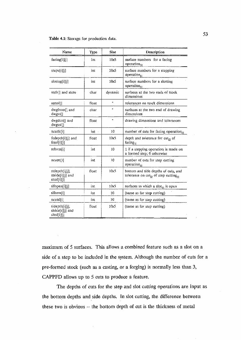
53 Table 4.1: Storage for production data.

Name ~ Size Description

facing[i][j] int 10x5 sruface numbers for a facing operation'il

stepc[i][j] int 1Ox5 surface numbers for a stepping operationm

sloting[i]lj] int 10x5 surface numbers for a slotting operationrll

stcfr[] and stcto char dynamic surfaces at the two ends of stock dimensions

stctol[) float " tolerances on stock dimensions

dwgfrom[] and char " surfaces at the two end of drawing dwgto[] dimensions

dwgdim[] and float " drawing dimensions and tolerances dwgtol[]

ncutfc[i) int 10 number of cuts for facing operationm fcdepth[i) [j) and float IOxS depth and tolerance for cut(jJ of fctol[i)UJ facing fll

stform[i] int 10 1 if a stepping operation is made on a formed step; 0 otherwise

ncutst[i] int 10 number of cuts for step cutting operationri]

stdepth[i][j], float lOxS bottom and side depths of cuts, and stside[ilUJ and tolerance on cutm of step cutting[i] sttol[i][j]

slfopen[i][j) int IOxS surfaces to which a slotfil is open

slform[i] int 10 (same as for step cutting)

ncutsl[iJ int 10 (same as for step cutting)

sldepth[iJUJ, float 10x5 (same as for step cutting) slside[ i][j) and sltol[i][j]

maximum of 5 surfaces. This allows a combined feature such as a slot on a

side of a step to be included in the system. Although the number of cuts for a

pre~formed stock (such as a casting, or a forging) is normally less than 3,

CAPPFD allows up to 5 cuts to produce a feature.

The depths of cuts for the step and slot cutting operations are input as

the bottom depths and side depths. In slot cutting, the difference between

these two is obvious -- the bottom depth of cut is the thickness of metal

54

. removed to form the bottom of a slot, and the side depth of cut is the

thickness of metal removed to form the side of a slot. In step cutting,

however, the bottom depth of cut is defined as the thickness of metal

removed to form the longer side of a step, and the side depth is the thickness

of metal removed on the other side of the step. Although it is realised that

the processing tolerance, which is the tolerance on the dimension of each cut,

depends on many factors such as the length dimension, the cutting depths, the

machining conditions, the condition of the machine-tool, and the operator's

skill, the tolerances of both depths are assumed to have approximately the

same value. This requires the user to use an appropriate mean value of

tolerance for both bottom cut and side cut.

The arrays which store the slot opening surfaces (slfopn[][]) are

required for the modification of the spatial representation model for various

shapes of the machined part. For example, if a slot is cut in a solid stock, the

slot has to be removed from the model so that it represents the condition of

the workpiece prior to the cut being made, that is the slot surfaces will be

required to merge. The array slfopen[][] serves this function. More details of

the procedure for changing the spatial representation model will be discussed

in chapter 6.

The arrays stform[] and slform[] store the flags to signify if a step or a·

slot is machined from a formed feature. This information is required for the

modification of the workpiece model, and for the input of the production

data. In the latter, if the flag is on, the bottom and the side cutting depths

together with the machining tolerance must be entered for the first cut;

otherwise, only the tolerance is required. Note that the tolerances of the

stock and not the dimensions are required by the system. CAPPFD will show

these dimensions in the tolerance charts. But, if stock dimensions are

· available, the user must work out the number of cuts and the cutting depths

from the stock dimensions and the finished part dimensions. In this case, the

results in the tolerance charts must agree with the stock dimensions.

4.6 Data input

EntH nIl' name for st(trinq data: wr.rk .d

I~ufflber of stork dimensions !type 0 if no ste,ck dilllel'lsil)n): 3 Enter stocK dimensions:-# 1:- stk. dim. frDID: 1

st\:. dim. to : b tolerance(aml: 0.15

t 2:- stk. di~. from:--7-­stk. dil. to :-rl tolerance!mml: 0~5

t 3!- stk. dim. from: 12 stl:. dim. to : 14 htierall!:e!mlllh 0.15

Humber of drawing dimensions: 10 Enter drawing dimension5~-~ j:- owg. Olill. fro~:~

dWQ. dim. to : ~ dimensirln(mm): 39.(10 tr,lerancP!IDm): 0.1(1

D E:- dWQ. dim. from:jl dwg. diu!. trl : 10 dil1lrmsionlmm}: 10.00 tr<ll'Tanrplmmh 0.(19

(a)

Enter the nUlilber tlf hdng openticlns \type 0 if m' facing operatil:.nl: l!:.

facing 11:- (type (I tD stDp) en surface: 1.a r'n surface:..Q. nu~ber Df cuts:JL rut t 1: dfpth rd cut lim): 5.0(1

mc trllEnncp lam): o.TIi cut t 2: depth rlf cut l!llm): 1.(1(1

me tDlerance IfIlm): 0.05 facing 1I2:- (type (I te, stc.p) -

rm surface: it on surface: J!.

number of cutSl cut j 1: depth cut (m,,): 5.00

mt tolerance (!lim): O,H\ cut 11 2: depth of cut (flln): 1.5

me tolerance (~~): 0.08 facing *3:- (type 0 to stop) ---­

[In surface: 1. tin surface: 2 on surtilce: (I

nUllbl:'T rtf cut!>: cut I 1: depth cut (rem): b.OO

mc tolerance (mm): O.lb

(b)

FIg.4.9: Dialogue for data input.

As mentioned before CAPPFD reads the spatial representation model

of the part from a data file, and interacts with the user for the production

data. Fig.4.9, shows examples of the dialogue for the input of: (a) stock and

drawing data, and (b) facing data. The data from this interaction are stored

in a data file under a name given by the user. During the dialogue, if there

are any mistakes in entering the data, the user cannot make the corrections;

but the corrections can be made afterwards in the editing session. The

editing routine provides three main types of editing: adding, deleting, and

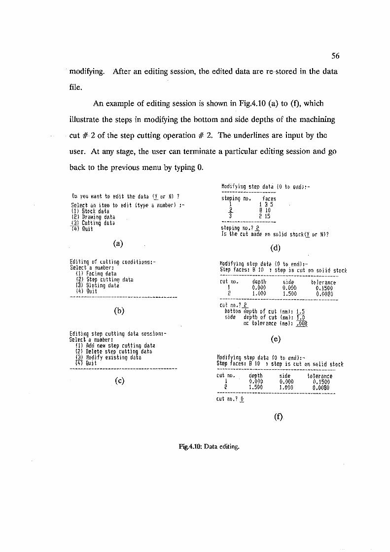
56

. modifying. After an editing session, the edited data are re-stored in the data

file.

An example of editing session is shown in Fig.4.10 (a) to (f), which

illustrate the steps in modifying the bottom and side depths of the machining

cut # 2 of the step cutting operation # 2. The underlines are input by the

user. At any stage, the user can terminate a particular editing session and go

back to the previous menu by typing O.

OJ) ve,u l'Iilnt to edit the dtltil eL or ill ? Select an item to ~dit !type il number) .­I, 1) St,.c\: datil (2) DrawinQ data 1,3} Cutting data l1i1 Guit

(a)

Editing of cutting cCtnditiolls:­Select a number}

(1) Fae ing data m Step euttimr data !3} Sll:<ting data ~4} QuH

(b)

Editing step cutting data s~5siCtn:­Select a number:

!I) Add new step cutting data (2) nelet~ step cutting data (3) Modify e~isting data m Quit

(c)

Kodifyingstep data 10 tel end):-

faces 1 3 5 B 10 2 15

stl'~i!ig no.? Is the cut [Ill 5t<lld sic,d!l "r in?

(d)

I1c.dHvlng step data iO te. end):-Step feces: B 10 : step is cut on solid stock --~---------------------------------~-~----cut no.

1 2

depth 0.000 1.000

side 0.00(1 1.5M

itdfrance 0.1500 (1.0(180

----------------------------~--------------cut no.? 2

bl'Jttl'till depth r.f cut (mm): 1.5 side depth of cut fmro}: ~

~c tolerance (mm): :UUB

(e)

K[tdlfyi1l9 step data fO te. endh-Step face!>: 8 10 : step is cut Oll sedid ste<el: ------------~------------------------------cut IlO,

t 2

side 0.000 1,0(10

tc<lerance 0.1500 0.0080

-----------------------------------~-------Cllt no,? it.

(f)

Ftg.4.10: Data editing.

57

. 4.7 Data output

The outputs from CAPPFD are:

(1) the sequence of machining operations,

(2) the locating surfaces on the workpiece for each operation, and

(3) the tolerance charts.

To save the computer memory, the outputs from the sequencing

module are stored in the same arrays of features (facing[][J, stepc[][], and

sloting[][D as the inputs. The only difference is the order in each array. In

other words, the positions of the row elements in each feature array are

changed by the sequencing module.

Table 4.2: Arrays for storing 3-2-1 location systems.

Name

loffc3(i][j). loffc2(i][j). int 10x5 3-. 2- and I-point loffc1[i)01 locating faces for facing

operation i •

locfc3[i][j)[k]. float 10x3x3 coordinates for placing locfc2[i)fj][k]. 10x2x3 3-. 2- and I-point 10cfc1(i][j] 10x3 locating symbols.

10fst3[i][j]. lofst2[i:101. lnt 10x5 locating surfaces for 10fst1[i][j] step cutting i .

10cst3[i][j][kJ, float 10x3x3 coordinates for locating locst2[i][j][k], 10x2x3 symbols. 10cstl[iJU] lOx3

lofsI3[iJUl. lofsl[i][j]. int 10x5 locating faces for lofsl[ iJm slotting i'

locsl3 [i]UJ[k]. float 10x3x3 coordinates for placing locsI2[iJl]][k], locsl[ i][j] 10x2x3 locating symbols.

10x3

For the locating surfaces, the data are stored in three arrays of floating

point numbers as shown in Table 4.2. Also shown in the table are the three

arrays for storing the coordinates of the location systems. These coordinates

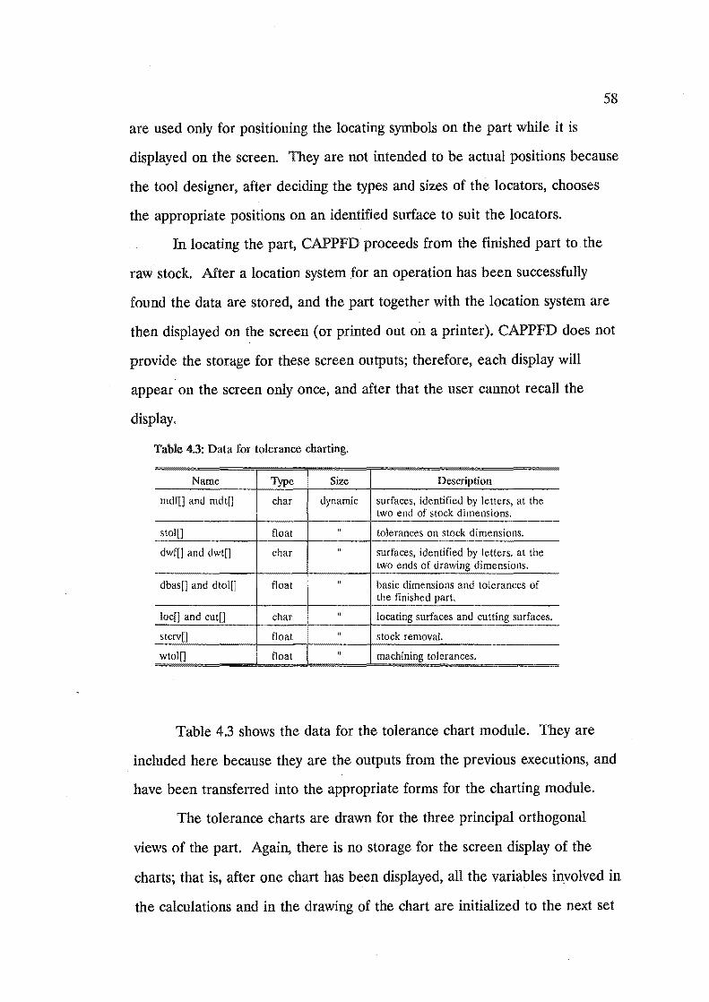
58

, are used only for positioning the locating symbols on the part while it is

displayed on the screen. They are not intended to be actual positions because

the tool designer, after deciding the types and sizes of the locators, chooses

the appropriate positions on an identified surface to suit the locators.

In locating the part, CAPPFD proceeds from the finished part to the

raw stock. Mter a location system for an operation has been successfully

found the data are stored, and the part together with the location system are

then displayed on the screen (or printed out on a printer). CAPPFD does not

provide the storage for these screen outputs; therefore, each display will

appear on the screen only once, and after that the user cannot recall the

display.

Table 43: Data for tolerance charting.

Name Type Size Description

mdf[J and mdt[] char dynamic surfaces, identified by letters, at the two end of stock dimensions.

stol[] float " tolerances on stock dimensions.

dwf[] and dwt[] char " surfaces, identified by letters, at the two ends of drawing dimensions.

dbas[] and dtoll:J float " basic dimensions and tolerances of the finished part.

loc[] and cut[] char " locating surfaces and cutting surfaces.

stcrv[] float " stock removal.

wtol[] float " machining tolerances.

Table 4.3 shows the data for the tolerance chart module. They are

included here because they are the outputs from the previous executions, and

have been transferred into the appropriate forms for the charting module.

The tolerance charts are drawn for the three principal orthogonal

views of the part. Again, there is no storage for the screen display of the

charts; that is, after one chart has been displayed, all the variables inyo!ved in

the calculations and in the drawing of the chart are initialized to the next set

59

of data, and the execution is then repeated.

4.8 Conclusion

CAPPFD may receive data in two ways, by directly reading a data file,

or by interacting with the user. All of the production data are stored in

arrays of one or two dimensions, and they are arranged in 'pairs'. That is, the

data relevant to the same feature or operation are identified by the same

index number. This concept makes the ~ata structures simple and helps

simplify the tolerance chart algorithm. The user has to prepare the

production data from the stock and drawing dimensions manually before

entering them into the system. Also the user is responsible for deciding the

appropriate values of the processing tolerances. The outputs from CAPPFD

are shown on the screen. To record the outputs, CAPPFD prints them on the

line printer.

60

. 5. MACHINING SEQUENCE PlANNING

Most of the CAPF systems, for prismatic parts, developed so far lack a

capability to generate the machining sequence; they are used mainly for

selecting cutting conditions, cutting tools, and machine-tools. Some do

incorporate such capability, but it is limited to only a certain kind of feature,

eg., a counter-bored hole, or an internal thread. There have been no reports

of attempts to sequence the machining operations based on the dimensional

relationship among features. It is in this respect that CAPPFD differs from

other systems. It is capable of generating the machining sequence

automatically; that is without any intervention from the user. This chapter

explains the development of the sequencing algorithm adopted in CAPPFD.

5.1

In computerized process planning, there are two basic strategies for

sequence planning: fOlward planning and backward planning. FOlWard

planning starts the sequence from a raw or stock shape and ends up with a

finished product shape. In this case, the number of surfaces on the workpiece

increases as more machining operations are performed. Backward planning,

on the other hand, works in the opposite direction; it starts from a finished

part and progresses towards a stock part, or from more surfaces to less

surfaces. Thus, in backward planning, the machining sequence required is the

reverse of that considered in the planning process. Backward planning,

however, offers advantages over forward planning, such as simplicity in

manipulating of the geometrical part model representation, less data storage

. required, and economy in execution [37].

The weak points of the existing systems that use both strategies are:

they are concerned only with the changes in the geometrical shape of the

workpiece, and no consideration being given to the dimensional control,

which is the most essential part of process planning.

61

CAPPFD utilizes the advantages of backward planning by

incorporating the concept in the routines for locating the workpiece, but it is

n~t used for sequencing the operations.

5.2 Basic sequencing concept

'Because the sequence of machining operations in quantity production

is based on where to locate the workpiece for machining, the feature that is

likely to be machined first is the one that has more potential to be used as a

locating feature for machining other features.

Normally, in machining, flat surfaces are machined before steps and

slots. This is because they can provide locating surfaces for other operations.

The face of a step can sometimes be used as a locating surface. However, it

is very rare that a workpiece is located from a surface of a slot. For these

reasons the general sequencing plan is that all flat surfaces are machined

before the steps; the steps are machined before the slots. There still remains

the sequence for machining the features of the same type. This sequence

depends on the following main factors:

(1) th~ number of dimensions on a feature relating to a certain type

of feature,

(2) the closeness of tolerances on dimensions relating to a certain

type of feature, and

(3) the degree of geometric' control that a feature can offer, if it is

chosen to be a locating feature.

For example, in the case of flat surfaces, if a flat surface has more

dimensions relating to other flat surfaces, that surface is to be machined

before the others; but, if a tie exists, the closeness of tolerances on

dimensions will be considered; then, if a tie still exists, the number of

dimensions relating to the steps will be considered. If all dimensional

relationships are equal, the priority will be given to the surface capable of

giving the highest degree of geometric control.

62

This concept is, therefore, based on the practicality of machining a

type of feature, and on dimensional and geometric control. In the following

sections, the detailed implementation of the concept is explained.

5.3 Ranking of machining operations

As discussed in chapter 4, three two-dimensional arrays, namely,

facing[][], stepc[](] and sloting(][], are used to store the surface numbers for

facing, step cutting and slotting operations respectively. These arrays can be

referred to as feature arrays or operation arrays, because each of them

contains the surfaces of the same feature type, and requires the same type of

operation.

To sequence the operations in a particular feature array, the row

elements of the corresponding array are swapped according to the criteria

outlined above, and when a swap is made all information pertaining to the

swapped features is also exchanged.

There are 2 steps in deriving the sequence for the operations of the

same type, ie, ranking and modifications. In this section, the focus is on the

first step.

63

Table 5.1: Data for operations sequencing.

Name Type Size DC""ll}1UUll

mcfn int dynamic surfaces requiring machining.

unmac[][] int dynamic unmachined surfaces.

relfc[i][] int lOx 10 surfaces dimensionally. relating to facer!]'

relst[i][J int lOxlO surfaces dimensionally relating to. stePm'

relsl[iJ[] int lOx 10 surfaces dimensionally relating to slotfil •

scfcli] int 10 number of dimensions relating to facefij.

scst[i) int 10 number of dimensions relating to stePm'

scsl[i] int 10 number of dimensions relating to slotril'

rankfc[i] int 10 ranking number of face rn .

rankst[i] int 10 ranking number of stePm.

ranksl[i] int 10 ranking number of slotm.

In ranking, some intermediate data, which have been derived from the

data input, are required. These data are stored in the variables listed in

Table 5.1. The ranking procedure starts by counting the number of

dimensions relating to a feature, and assigns that number to the

corresponding score arrays (scfcn, scst[] or scsl[]). Then, the elements of the

score array are sorted in a descending order. During sorting, any swap of the

elements in the score array will cause the related data to swap accordingly.

After this, each operation is given, based on its score array, a ranking

number: the higher the rank the earlier the feature is to be machined. The

ranking numbers ~re stored in three one-dimensional arrays (rankfc[], rankst[]

and ranksl[]) corresponding to the three feature types. The maximum

possible integer value to be assigned to the elements of each ranking array

depends on the number of operations of the same type. For example, if there

are five facing operations, the maximum ranking value will also be five. When

64

a tie exists, all the elements in the ranking array corresponding to the tied

operations are assigned the same number. For example, if scfc[iJ ::::: { 2, 2, 1,

1, 0 }, where i::::: 1,2 ... 5, then rankfc[iJ ::::: { 5, 5, 3, 3, 1 } . Note that scfc[5] = 0

does not mean this surface has no dimensional relationship with the other

features, but ~it means the this feature is dimensionally referenced by features

that do not require machining. Fig.5.1 shows a simplified flowchart for

ranking facing operations. The same logic is used for ranking other

operations. Also note that the relationship arrays (relfc[][], relst[][] and

relsl[][]) store the surface numbers of the surfaces that are dimensionally

referred to by a feature. These surfaces are either those requiring or not

requiring machining.

tar

~ount the number of

non-zero elements in array relfe[i] which are the surfaces that' require machining.

"'-_---.::NO"-< All i ?

Yes Sort array sefe[} in descending order, and swap row elements of array facing!) [J and other data relevant to the rows accordingly

Assign a ranking number to rankfc [iJ ..

FJg5.1: Flowchart for ranking facing operations.

65

. 5.4 Sequence modifications

After ranking, some operations may have the same ranking number.

That is to say, from the baseline demensioning point of view, they are equally

qualified for being machined at the same time, which is not possible in the

case in conventional milling operations. Therefore, further modification of

the sequence is required for those operations having the same ranking

number.

Since a slot is not. used for locating the workpiece, the rules for

modifying the sequence of slotting operations are different from those for

facing and step cutting.

The flowchart in Fig.5.2 shows the procedure for modifying facing

operations. It starts by first assigning the number of facing operations to an

integer variable, 'val' (box 1); 'val' must start from this value

because it is the maximum ranking number. Then, the elements in array

rankfen which are equal to 'val' are counted, and the result is assigned to a

variable 'sum' (box 2). If 'sum' is more than 1, it means there are more than

one elements in array rankfc£] that is equal to 'val', so the operations

corresponding to these elements require reshuffling. In box 3, the variables,

which are the factors for this reshuffling, pertaining to facer!] are searched or

calculated. Box 4 shows similar variables for facefj]' Based on these factors,

the decision table in box 5 decides if a pair of operations needs swapping. It

should be noted here that the first 6 factors in box 3 are concerned with

dimensional control; the last, with geometric control, and that the conditions

in the decision table are evaluated sequentially. This means if two features

can equally provide the same degree of dimensional control, their sequence is

then based on the geometric control criterion -- the area bounded by the

66

~ 1. val - number of I

facing operations , 2. Count elements in lI.r:ray rankfc []

that are equal to 'val': and assign the number to 'sum'

No ~ Yes 3. For facing[i];

search for or calculate: QJ no. of dims. from face [i] to

other flat surfaces (no_il; @ smallest tolerance on dims. from

face [1] to other flat surfaces (toli) ; Q> no. of dims. from face [i] to

other step surfaces (stepi); ® smallest tolerance on dims. from

face [i1 to other step surfaces (tolsti); ® no. of slot sides related to face[iJ

(sidi); @J smallest tolerance on dims. from

slot sides to face[i] (tolsli) ; (J) area of face [iJ (areai) . ..

j = i+11 'f

! 4. For facing[j]:

I search for,?r calculate:-no j I tolj, stepj, tolstj I sidj, tolslj, and areaj

5. •

CONDITION STUB ~NDITI0W,'Y e .,

! no_i < no.J 0 0 0 Ii· ;+1 1 no_i - no.J n 1 1 1 1 1 toli > tolj n 1 0 0 0 0 (J + toli m tolj n n 1 1 1 ~K- j <-1 sum stepi < stepj mn

I-1 0 0

i stepi m stepj n n 1 1 1 1 No t018ti > tolstj n n n 1 0 0 0 lim i+1 I to1sti m tolstj n n n n 1 1 1

.1di < sidj min 1 0 0 Yes : sid! - sidj n n n 1 ~ to18li > tols1j n n n n 0 l-

I tol.11 - tal,,, n Inn ~w::: No

areai < areaj n n n n n 1 6. Assign new numbers ACTION STUB ACTION ENTRY to rankfc[vall, ... swap i, j x'x x x x x x )J-. rankfc[val-sum] • no swap ~t

I val· val-l 1

~Y •• vall- 1

No op

Fig5.2: Flowchart for modifying facing sequence.

surface with three point-locators. When all 'sum' operations have been

reshuffled, new ranking values are assigned to those operations (box 6) so

that they do not have the same ranking value.

The flowchart for modifying sequence of step cutting operations is

similar to Fig,s.2 except that all data pertain to the steps; it is not shown

here.

67

However, the procedure for modifying the slotting sequence needs

some explanation. Though the logic is, in general, the same as for the facing

and step cutting operations; since a slot is not used for locating the part, the

criteria for evaluating the sequence are based only on the dimensional control

of the part. Fig.5.3 shows the flowchart, and the criteria are listed in box 3.

The general idea behind these criteria is that a slot which has a relationship

of higher importance in dimensional control should be given a higher priority,

being machined before the others, so that it can provide a more accurate

gauging reference in the inspection of other slots. The factors are listed

according to the order of importance of the factors; the more important ones

come first. The rules in the decision table in box 5 are executed sequentially

as in the case of facing.

5.5 Adjustments for combined slots

A combined slot is a slot which contains one or more other slots. Slots

-3 and 5 in Fig.5.4are examples of the combined slot; slots 3 has slot 0 at its

bottom face, and slot 5 contains another two slots. In practice, the slots closer

to the top surface are normally machined before the lower ones. The reasons

for this are: it is faster to machine because larger cutter can be used for the

slots on the top, and a more uniform cutting action can be maintained.

= rhj

2. Count elements in array ranksl[1 that are equal to 'val'; and assign the number to 'sum'

3. For s

no. flat surfaces related (no_i); @ the highest ranking number of

flat surfaces related (rhi); CY no. of step surfaces related (stepi); GD the highest ranking number of

step surfaces related (rhst!);

rhstj

stepi < stepj ; step! stepj rhsti < rhstj

ACTION STUB SWAP i, j

NO SWAP

Yes

6. Assign new numbers to ranksl[vall, ••. ranksl[val-sum).

FJg53: Flowchart for modifying slotting sequence.

68

69

As the sequencing module treats a combined slot as two or more

individual slots, the sequence obtained may have a lower slot machined

before the upper one. This requires some adjustments so that the sequence

will comply with practice.

A subprogram was written to adjust the slotting sequence. It makes

use of the surfaces to which a slot is open (slfopen[][]) to indicate if the slot is

a lower slot. slot. If so, that slot is cut after the upper one. Then, the row

elements in slotting array corresponding t? the upper slot are shifted to be in

front of those corresponding to the lower slot. For instance, supposing the

slotting sequence in Fig.5,4 is { 0, 1, 2, 3, 4, 5 }. That is, slot # 0 is machined

before slot # 1, slot # 1 before slot # 2, etc. The slot numbers are

surrounded by a circle in the figure. After the adjustment, the sequence will

become { 3, 0, 1, 5, 2, 4}. Fig.5.5 is the flowchart showing the logic for

adjusting the slotting sequence.

Whenever there is a swap of operations in the sequence either in the

ranking, the modifying, or the adjusting phrase, all other relevant data are

also swapped.

22

23

24

FJg5.4 Combined slots.

2. Exchange row elements of array sloting[] [I:

No

Q) store elements of row i in a temporary storage;

® shift elements from row i to IOW (j"l) further one lOW;

ill Ie"store the elements in the temporary storage into row i.

No

i (BU. [0iJ

FJg55: Flowchart for adjusting slotting sequence.

5.6 Calculation of surface locating area

70

CAPPFD uses the triangular locating area (the area surrounded by

three point-locating pins) as the means for measuring the degree of geometric

control; the larger the area is, the better geometric control it can offer. The

area may cover more than one surface on the same level, and it may be a

machined or an unmachined surface. Examples of these surfaces are shown in

Fig.5.6.

To calculate a triangular locating area, for instance, on surfaces d and

e in Fig.5.6, first, the coordinates of the extreme edges: 1-2, 2-3, 4-5, 5-6 and

71

·7-8, of the surfaces are stored temporarily in three one-dimensional arrays (x-,

y- and z-coordinates are stored separately). Then, these arrays are used to

calculate the triangular areas formed by the coordinates of three points. And,

finally, the largest area is chosen to be the surface locating area. The same

procedure is also applied to calculating of the locating surface on a side of a

step.

~--Btep

flat faces

2

FJg.5.6: Examples of locating areas.

5.7 Conclusion

All facing operations are carried before step cutting operations, and

the step cutting operations are performed before slotting operations. The

sequence of the operations of the same type is based on the baselines for

dimensioning, closeness of tolerances, the relationships to other types of

features, and the triangular locating areas. Dimensional control over the

workpiece is the primary objective of the sequencing routines.

72

. 6. WCATION SYSTEMS

The location system adopted in CAPPFD is the well-known 3-2-1

location system, which is accomplished by placing 3 locators on the largest

surface, 2 locators on the second largest, and 1 locator on a surface

perpendicular to the first two. This is a theoretical location system which is a

result of the workpiece control analysis. The tool designer is responsible for

transforming it to a physical system that satisfies the theoretical requirements.

It can also act as an input to an automatic fixture design system such as that

described by Ngoi [52].

CAPPFD produces the location system for machining each feature in a

form of 'process pictures' which can be used as a basis for the tool designer to

identify the appropriate locating surfaces. In this chapter, the algorithm for

locating the workpiece is discussed.

6.1 Process picture

A process picture is a piece of information concerning how a

workpiece is to be located, supported, and clamped for machining. It is a

means for transmitting the ideas from the process planner to the tool

designer. It describes the workpiece as it appears just after an operation has

been completed. Normally, a process picture contains information such as the

drawings of the workpiece, the processing dimensions, the feature to be

machined, and the symbols indicating the locating, supporting, and clamping

points.

However, in CAPPFD, a

simplified process picture, as

shown in Fig.6.1, is used. The

surfaces are identified by

numbers. All processing

73

dimensions are omitted because ,...\]-"--------"--,

the outputs from the package

include a set of tolerance charts

which show all of these

dimensions. The locating

surfaces are indicated by

triangular symbols.

4.

6.2 Backward planning: the application

Feature being machined, face, 1

Ftg.6.1: A process picture.

As mentioned in chapter 5 CAPPPD makes use of backward planning

in locating the workpiece. The first operation for which the locating module

searches for the location system is the last operation in the sequence, ie, one

of the slotting operations. At this stage, all surfaces on the part, except those

belonging to the slot being machined, are candidates for being locating

surfaces. After the part has been successfully located, the model is modified

so that it represents the geometry of the part just before the slot was

machined. The modifications are also made on the surfaces numbers in

varioQs arrays that store them. (This will be discussed later in this chapter.) .

CAPPFD, then, extracts the coordinates of the surfaces of the new model and

store them in the same variables that have been used before. Then, the

locating procedure continues for the second last operation. This process is

repeated until all location systems for all operations have been found; that is

. the process ends when the workpiece becomes a stock part.

6.3 Type of locating surface

On a machined part presented for locating, there are two types of

surfaces; machined and unmachined surfaces. The machined surfaces are

those having been machined previously, in the earlier operations. The

unmachined surfaces are either surfaces that require machining but are not

yet machined or those do not require any machining.

74

In backward planning of the location systems, the number of

unmachined surfaces increases as the planning goes on, because some of the

machined surfaces change to unmachined surfaces. To demonstrate this,

consider the following: having completed locating the workpiece for a facing

operation, the locating module identifies all the surface numbers just

machined as the unmachined surfaces, and adds them to the unmachined

feature array (unmac[][]). In the case of a step, it depends on whether the

step cutting is cut on a pre-formed step or from solid stock. If it is cut on a

pre-formed step, the step surface numbers will be transformed to the

unmachined feature array. But, if it is cut on solid stock and the surface of

the solid stock at that particular region does not requires further machining,

no transformation is made. After this, the transformed surface numbers will

also be eliminated from the array storing the machined surfaces (mcf[]).

CAPPPD gives a higher priority to the machined surfaces in locating

the workpiece.

6.4 Slot base and step base

The concept of 'slot base' and 'step base' is introduced into the

CAPPPD system to decide the position of the cutting tool relative to a slot or

75

. a step being cut. This concept is essential for the input of depths of cut for

machining both features, as well as for locating the workpiece -- in the case of

a slotting operation.

slot side

slot side se

(a) slotting (b) slotting

machined face ste side

(c) step cutting (d) facing

FJg.6.2: Slotting, step cutting and facing operations.

The slot base is defined as the bottom surface of a slot. While it is

being machined, this surface is always facing to the milling cutter, either an

end mill or a side and face mill, as shown in Fig.6.2. It follows that the

surface which is parallel to the slot base and is on the same side as the

cutting tool will never be used as a locating surface for cutting the slot.

Although the concept of step base is concerned only with types of

cutting relating to depths of cuts for a step, which is part of the input data, it

is found appropriate to discussed it here, for it relates to the relative position

of the cutting tool. Normally, in machining a step, the operator tries to

minimise the distance the tool moves while cutting by feeding the tool in a

76

. direction parallel to the shorter side of the step, so that the step can be cut

faster. In Fig.6.2(c), the step base would be regarded as the longer side of a

step.

Regarding the locating surfaces for machining a step, no surface on the

same side as the cutter can be used as a locating surface.

The following are the a summary of the rules for identifying the

locating surfaces:

(1) In facing operation, the surfaces that are parallel to and with

normals pointing to the same direction as that of the surface(s)

being cut are not used for locating.

(2) In cutting a slot, the surfaces that are parallel to and with

normals pointing to the same direction as that of the slot base

are not used for locating the workpiece.

(3) In cutting a step, the surfaces that are parallel to and with

normals pointing to the same direction as those of the step sides

are not used for locating.

In applying the concept to depth of cut, the bottom depth is the

amount of metal to be removed to produce the slot or step base, and the side

depth is, to produce the side of the slot or step.

6.5 Searching for locating surfaces

Before a search for a location system for an operation can be made, all

the qualified locating surfaces, machined and unmachined, are first searched

and stored in two one-dimensional arrays of 'structure', larea[] and ularea[],

as listed in Table 6.1. The procedure for searching for machined or for

Table 6.1: Temporary storage for locating areas.

Name Type Size

lareal] structure' dynamic

luarea[] structure' dynamic

stores all machined surfaces that may be used for locating the part for an operation

stores all unmachined surfaces that may be used for locating the part for an operation

• NOTE: Structure is another type of variable in C. It consists of several members which can be of different data types, and it is given a name for referencing. The structure 'ainfo' is created for larea[] and luarea[]; it has the following members:

struct ainfo { float area;

int facerS]; float x[3]; float y[3]; float z[3];

unmachined locating surfaces are basically the same. The only difference is

the data involved in the procedure.

77

The flowchart in Fig.6.3 shows the general steps in searching for all

possible machined surfaces qualifying for locating a workpiece for machining

a slot.

The procedure starts with those surfaces requiring facing operations. If

they have been previously machined and are parallel to and not facing the

same direction as the slot base, they will be stored in larea[]. Also at this

time the triangular locating area is calculated. This area and its coordinate

are then stored in larea[], under different member names. When all surfaces

from facing operations have been considered, the same process is repeated

for the step surfaces.

The arrays larea[] and luarea[] are both temporary storage in the sense

that once a location system has been found from them, their memory

locations will be freed, and will be re.,allocated again when required.

2. Search for flat surfaces that require facing operation[i] •

3. ave

they been machined

? Yes

4.

No

No

5. Calculate 3-point locating areal store the area, coordinates, and face numbers in larea [j]

Yes

Increment i by 1

6. Repeat steps above for surfaces l:equil: step cutting

78

F'Jg.63:Flowchart for searching for the machined surfaces for locating the workpiece in slot cutting.

6.6 Searching for a location system

The first step in the process of searching for a location system is to

sort the arrays laera[] and luarea[] in a descending order of the locating areas.

The following logic is then applied:

(1) Search the machined locating surfaces; if no appropriate faces

are found for a system, the unmachined locating surfaces are

then searched.

10.

luarea [J, and sort in descending order of areas

2. SeaIch latea!) for 3-point locating faces

3. No Yes, one of laxea!) found

r'f----< o1f Yes, the last

available .4. Search luarea[J

for 3-point locating faces

faces found

11. Search larea!l for 2-point locating faces

5. No

No Yes, one of larea!) found

6. Search luarea [] for 2-point locating faces

7. No

Yes, the last available

faces found 13. Search larea!] for l-point locating faces

14. No

Yes ~----------~L-----~-<found ?

B. Search luarea[) for 1-point locating faces

No

Yes

, Print message, and terminate i the program stop

Ftg.6.4: Flowchart for determining a location system.

(2) If location system can be partially found -- eg, only 3-point, or

3-point and 2-point locating surfaces -- from the machined

surfaces, the search is switched to the unmachined surfaces.

79

80

(3) Whenever the lists of the locating surfaces are exhausted and a

complete location system can not be found the procedure prints

a message and terminates the program.

1. Check 1area[i]; if any of facer] is related to the slot conside::ced

Yes

No

r----~----<:are they 7

Yes f.,-------<:are they

?

2. Return value i indicating that 3-point location is found

No all i >-__ N_O __

?

Yes

5. Return a value indicating that 3 -point location: is not found

Ftg.65: Flowchart for determining a locating area for a slot machining.

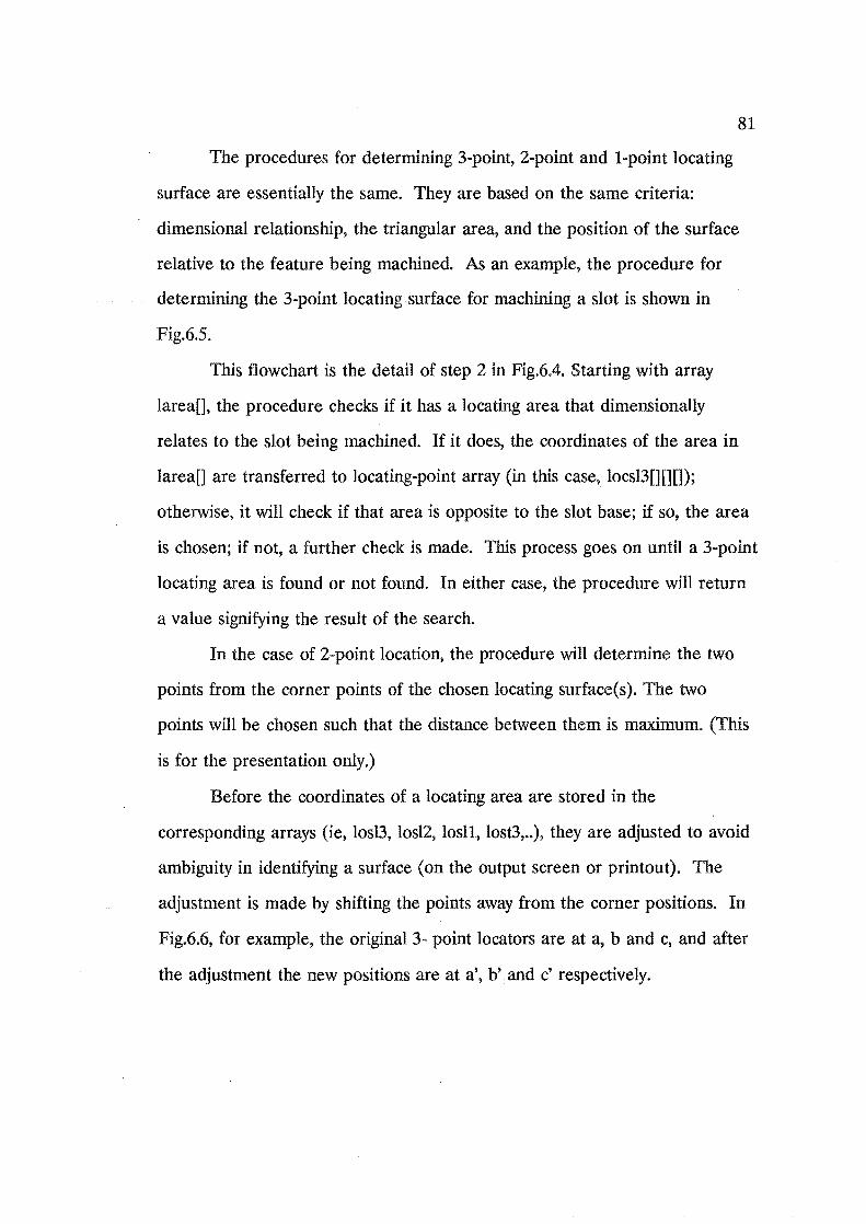
81

The procedures for determining 3-point, 2-point and I-point locating

surface are essentially the same. They are based on the same criteria:

dimensional relationship, the triangular area, and the position of the surface

relative to the feature being machined. . As an example, the procedure for

determining the 3-point locating surface for machining a slot is shown in

Fig.6.5.

This flowchart is the detail of step 2 in Fig.6.4. Starting with array

larea[], the procedure checks if it has a locating area that dimensionally

relates to the slot being machined. If it does, the coordinates of the area in

larea[] are transferred to locating-point array (in this case, 10csI3[][][]);

otherwise, it will check if that area is opposite to the slot base; if so, the area

is chosen; if not, a further check is made. This process goes on until a 3-point

locating area is found or not found. In either case, the procedure will return

a value signifying the result of the search.

In the case of 2-point location, the procedure will determine the two

points from the corner points of the chosen locating surface(s). The two

points will be chosen such that the distance between them is maximum. (This

is for the presentation only.)

Before the coordinates of a locating area are stored in the

corresponding arrays (ie, losl3, losl2, 10sl1, 10s13, .. ), they are adjusted to avoid

ambiguity in identifying a surface (on the output screen or printout). The

adjustment is made by shifting the points away from the corner positions. In

Fig.6.6, for example, the original 3- point locators are at a, b and c, and after

the adjustment the new positions are at a', b'.and c' respectively.

a

a'

h

.. :3 point-locators

~ 2 point-locators

1 point-locator

FIg.6.6: Positions of locating symbols.

6.7 Graphical output of a location system

82

c

Fig.6.7 shows an example of the screen output resulting from the

locating routines. This is the 3-2-1 location system for machining the slot in

the bracket in Fig.4.1. The slot is identified by surface numbers 9, 10, and 3.

The 3-point locating symbols are on face 14, 2-point on face 6, and 1-point on

face 7.

After CAPPFD has completed one location system and before it

repeats the same procedure for the next operation, the representation model

must be modified so that the model represents the part geometry prior to the

operation just considered. For instance, if a slot in Fig.6.7 is machined from

a solid stock, then the slot does not exist before this operation, and the model

must be modified accordingly.

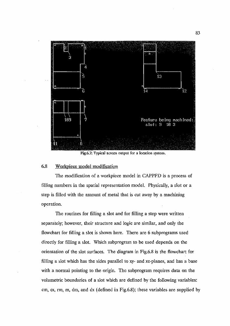
Ftg.6.7: Typical screen output for a location system.

6.8 Workpiece model modification

The modification of a workpiece model in is a process of

filling numbers in the spatial representation model. Physically, a slot or a

step is filled with the amount of metal that is cut away by a machining

operation.

83

The routines for filling a slot and for filling a step were written

separately; however, their structure and logic are similar, and only the

flowchart for filling a slot is shown here. There are 6 subprograms used

directly for filling a slot. Which subprogram to be used depends on the

orientation of the slot surfaces. The diagram in Fig.6.8 is the flowchart for

filling a slot which has the sides parallel to xy- and xz-planes, and has a base

with a normal pointing to the origin. The subprogram requires data on the

volumetric boundaries of a slot which are defined by the following variables:

em, ex, rm, rx, dm, and dx (defined in Fig.6.8); these variables are supplied by

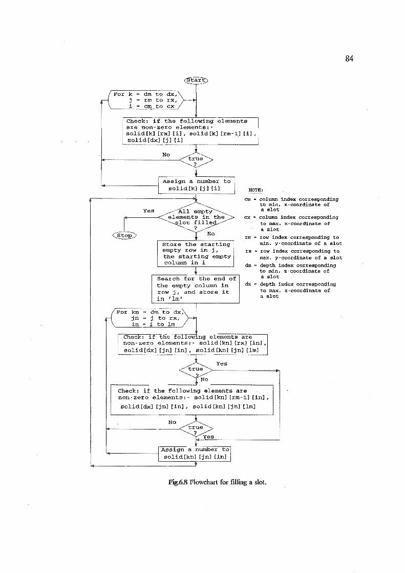
dm to dx, j rm to rx, i "" em to ex

Check: if the following elements are non-zero elements:-' solid[k] [rx] [i], solld[k] [rm-1] [1], solid[dx] [j] Ii] '.

Yes

No

to

Store starting empty row in j, the starting empty coltunn in i

Search for the end of the empty eoltunn in row j, and store it in '1m'

kn ~ dm to dx, j to IX,

i to 1m

NOTE:

em • column index corresponding to min. x-coordinate of a slot

cx • column index corresponding to max. x-coordinate of a slot

rrn Q row index corresponding to min. y-coordinate of a slot

rx • row index corresponding to max. y-coordinate of a slot

dID m depth index corresponding to min. z-coordinate of a slot

dx = depth index corresponding to max. z-coordinate of a slot

Check: 1f the followlng elements are non- zero elements I - solid [kn] [rx] [in) , solid [dx] [jn] [in], solid [kn] [jn] [1m]

Yes

Check: if the following elements are non-zero elements I solid [kn] [rm-1] [in],

solid[dx] [jn] [in], solid[kn] [jn] [1m]

Flg.6.S Flowchart for filling a slot.

84

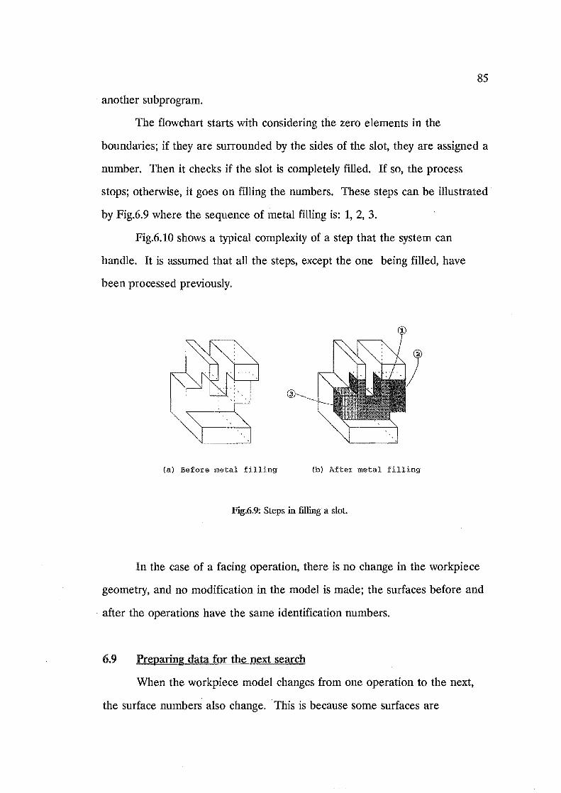
85

. another subprogram.

The flowchart starts with considering the zero elements in the

boundaries; if they are surrounded by the sides of the slot, they are assigned a

number. Then it checks if the slot is completely filled. If so, the process

stops; otherwise, it goes on filling the numbers. These steps can be illustrated·

by Fig.6.9 where the sequence of metal filling is: 1, 2, 3.

Fig.6.10 shows a typical complexity of a step that the system can

handle. It is assumed that all the steps, except the one being filled, have

been processed previously.

(a) Before metal filling (b) After metal filling

FIg.6.9: Steps in filling a slot.

In the case of a facing operation, there is no change in the workpiece

geometry, and no modification in the model is made; the surfaces before and

. after the operations have the same identification numbers.

6.9 Preparing data for the next search

When the workpiece model changes from one operation to the next,

the surface numbers also change. . This is because some surfaces are

86

(a) Before metal filling (b) After metal HIring

YJg.6.10: Metal filling of a step.

combined and some are eliminated. Therefore, it is essential to keep track of

the changes of these surface numbers. CAPPPD uses a two-dimensional

array, named track[][], to record the changes. It is created after the

sequencing of operations is completed. Fig.6.11 illustrates the idea of storing

the surface numbers in the array. The numbers circled indicate the sequence

of locating the workpiece. The surface numbers in column 1 belong to the

finished part which are used for locating the workpiece in the last operation;

those in column 2 are for, the second last, and so on. Note that a zero is

used for the array element to indicate that the particular surface does not

exist.

CAPPPD uses this array to modify the surface numbers in the arrays

involved in the search for a location system for the following operation.

These arrays include the feature arrays (sloting[][], stepc[][], facing[][]),

relationship arrays (relsl, reIst, relfc), machined surface array (mcf[]), and

unmachined surface array (unmac[][]).

In the end, these arrays will contain the surface numbers corresponding

to those of the stock. But, in drawing the tolerance charts, which is the final

7

8

2

4

5

5

4

5

1

(a) Finished part for slotting

(b) Part for step cutting

1

- ~2 (c) Part for

facing the top face

1

(d) Stock part

2

3

6

3

® 6

)Z 0

1

2

3

4

5

6

7

e

9

10

11

6

3

2

® 0 1 2

1 1 1

2

* I 3

4 0 0

5 3 2

6 4 3

7 5 4

8 I 6 5

9 6 5

10 0 0

11 7 0

12 8 6

(e) track[] []

FJg.6.11 The changes of model surfaces.

@ 3

1

0

0

0

2

3

4

5

5

0

0

6

step of the program, the original surface numbers are required for some of

these arrays. Therefore, a temporary storage is provided for storing these

surface numbers before the execution of locating module, and, afterwards,

87

88

. they are re-stored back, to the original arrays, for the charting module.

6.10 Conclusion

The procedure for locating the workpiece during machining is based on

both geometric control and dimensional control. All surfaces that are

candidates for being a locating surface are considered in order of their degree

of geometric control --the triangular locating areas, and in choosing a

candidate, the procedure gives a higher priority to one with a higher

requirement for dimensional control. That is, CAPPFD tries to maintain

dimensional control with the highest probability of achieving the best

geometric control.

89

"7. TOLERANCE CHARTING IN CAPPFD

Most computerised tolerance charting packages are limited to

rotational parts, which can be described by a two dimensional model, and

only one chart is normally required. Although the idea of charting the

machining sequence on a prismatic part is not new, so far there has not been

a published report on an attempt to computerize it. The CAPPFD system is

capable of producing the tolerance charts for all machined surfaces on a

prismatic part. At present, linear dimensional tolerances only are allowed.

The charting module in CAPPFD is a result of integrating the

tolerance charting program, discussed in chapter 2, with the sequencing

package. This chapter discusses some of the important details of the

integration.

7.1 Tolerance chart module

Fig.7.1 shows the flowchart for tolerance charting in the tolerance

chart module. This flowchart is basically similar to the one in Fig.2.6 except

that it has three new functions added. They are:

(1) A program loop for repeating execution: This enables CAPPFD

to produce three tolerance charts for a particular part. Each

time the loop is executed, it produces a tolerance chart for all

machining cuts made on the surfaces perpendicular to a

principal plane defined in the spatial representation model

(section 4.1). After the execution is completed, a new set of

data is required for the next loop execution. .

working dimension

For all cuts

4. create a path between the two cut faces of the stock removal

5. Calculate tolerance stack, on stock removal

For all resultants

6. Create a path from the two ends of a drawing dimension

7. Calculate the tolerance ~----------~ stack on a resultant

For all resultants

8. Create a path from the I two ends of a drawing dimension

9. Calculate a resultant dimension

10. Output the chart on

the screen (and on

a line-printer)

All three charts ~N __ o ____________ ~

completed ?

Ylg.7.1: Flowchart for tolerance chart construction.

90

91

(2) The data preparation function: This function embraces the

selection and organization of the data so that they can be used

for charting. In the following section the detail of steps in

preparing the data will be discussed further.

(3) The chart drawing function: This function is to draw the

tolerance charts on the screen; it is mainly supported by the

subprograms in the support module.

7.2 Data preparation for tolerance chart module

On a rotational machined part, the cut and locating edges that

establish the length dimensions are perpendicular to the work axis. Since

diametral dimensions are not normally charted, only one tolerance chart is

required. But, in the case of a prismatic part, where no axis of symmetry

exists, the machined surfaces contribute to length dimensions and tolerances

in more than one plane. Consequently, more than one chart is required for

analysing all dimensions.

To construct a tolerance chart for a set of dimensions, the tolerance

chart module needs only the data relevant to the dimensions. But, in

operations like step cutting or slotting, the surfaces in more than one plane

are cut, and there are three locating faces. As each machining cut in the

chart requires only one machined surface and one locating face, those

unrelated surfaces must be screened out.

The screening process in CAPPFD makes use a two·dimensional array

of integers, called map[][], which is temporarily created for each chart. This

array stores the surface numbers on different levels of the spatial

representation modeL Fig.7.2 illustrates an example of what is stored in the

array when the tolerance chart is to be constructed for the dimensions on the

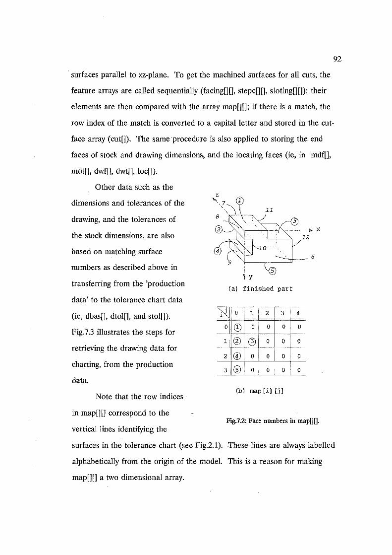
92

. surfaces parallel to xz-plane. To get the machined surfaces for all cuts, the

feature arrays are called sequentially (facing[][], stepc[][], sloting[][]): their

elements are then compared with the array map[][]; if there is a match, the

row index of the match is converted to a capital letter and stored in the cut­

face array (cutm. The same· procedure is also applied to storing the end

faces of stock and drawing dimensions, and the locating faces (ie, in mdf[] ,

mdt[], dwf[], dwt[] , loc[]).

Other data such as the

dimensions and tolerances of the

drawing, and the tolerances of

the stock dimensions, are also

based on matching surface

numbers as described above in

transferring from the 'production

data' to the tolerance chart data

(ie, dbas[], dtol[], and stol!:]).

Fig.7.3 illustrates the steps for

retrieving the drawing data for

charting, from the production

data.

Note that the row indices

in map[][] correspond to the

vertical lines identifying the

(a) finished part

tZ 0 1 2 3 4

0 0 0 0 0 0

1 ® @ 0 0 0

2 @ 0 0 0 0

3 ® 0 0 0 0

(b) map[i][j]

Ftg.1.2: Face numbers in mapU[].

surfaces in the tolerance chart (see Fig.2.1). These lines are always labelled

alphabetically from the origin of the model. This is a reason for making

map[][] a two dimensional array.

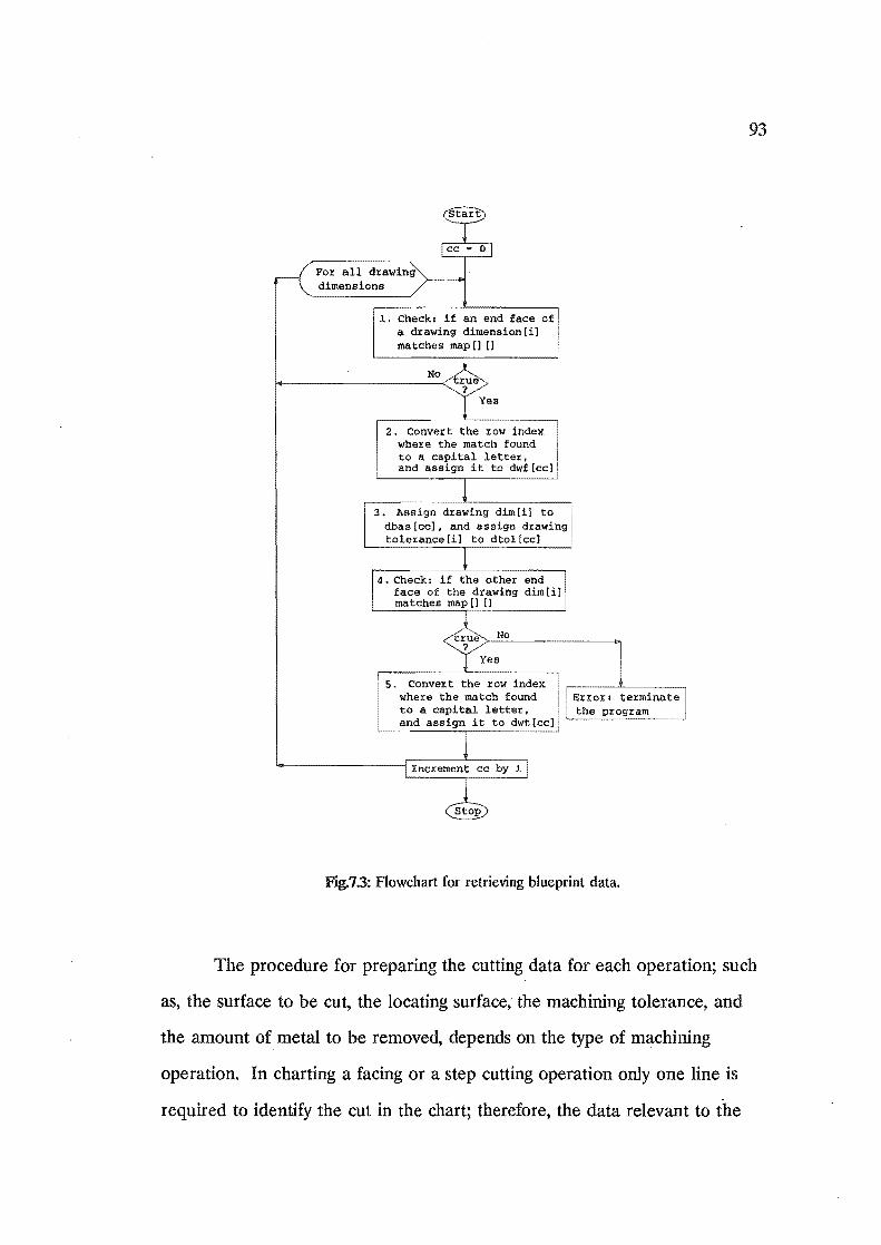
Foz all dzawing dimensions

1. Check: if an end face of a d~awing dimension[il matches map [] [1

No

2. Convert the zow index wheze the match found to a capital lettex, and assign it to dwf[ccl

3. Assign drawing dim [i] to dbas[cc], and assign dxawing tolexance[il to dtol[cc]

4. Check: if the other end face of the drawing dim[il matches map [] []

No

Yes

5. Convezt the row index wheze the match found : Error: terminate to a capital letter. the program and assign it to dwt[cc],

F'Jg.73: Flowchart for retrieving blueprint data.

93

The procedure for preparing the cutting data for each operation; such

as, the surface to be cut, the locating surface; the machining tolerance, and

the amount of metal to be removed, depends on the type of machining

operation. In charting a facing or a step cutting operation only one line is

required to identify the cut in the chart; therefore, the data relevant to the

. cut can be readily retrieved from the production data. But in charting a

slotting operation where the two

sides of a slot are charted, two

lines of cut are required, and

they are treated as two different

cuts in the chart as illustrated in

Fig.7.4. In this case, the

procedure must supply the data

for the extra cut, which can

occur simultaneously with the

other in some cases. Also

shown in the figure are two

methods of charting a slot: (a)

when the locating face is lower

than the cut face, and (b) when

it is higher. The reasons for

them are: firstly, in setting up

..... 'Z:_._.-,--_,.-._._._._.-.----_-, 0

I

(a) ty

z ..,.-._._.- .-.-.-.-.-.-----,0

(b)

F'Jg. 7.4: Charting a slot.

the cutter, the cutter side which is closer to the locating face is used.

94

Consequently, the arrow head of the cut symbol in the chart points to the side

of the slot closer to the locating face. Secondly, the width of the slot is either

a copy of the cutter width or a result of the movement of the cutter to a stop.

In both cases, the closer side determines the position of the other side;

therefore it should be the reference of the other side.

Fig.7.S and Fig.7.6 show the procedure for retrieving the cutting data

from slotting operations. The flowchart in Fig.7.S is for the case when the cut

surface is the bottom face of a slot. As each cut is represented by one line in

the tolerance chart, the transformation of data is straight forwards; the metal

For all slots>-----------~

2. Assign face number of slot base to 'bal'

3. Assign face numbers of slot sides to 'sdll' and 'sdl2' such that sdl1 < sd12

4. bsl

No matches map[c] []

?

>--------II{A

For all cuts made on slot til

Yes

5. Convert column index, c, to a letter and assign it to cut [n2)

6. Any

locating No

(in Fig.? .6)

face matohes >-------------------~ map [01] [}

?

Yes

? Conve~t column index, 01, to a letter and assign it to loc [n2]

B. Assign: QD bottom depth of cut to stcvr[n2], ~ slotting tolerance to wdtol[n2), @ a SIGN for cut [n2]

~------------------~B

Fig. 7 5: Retrieving chart data from slotting operations.

95

sdll No matches

map [c2] [] ?

Yes

10. sd12 No matches

map [c3J [J ?

11-Y

locating No face matches

p [c4] [] ?

Yes E:£l:or: terminate 12. program

Yes ocating No

face < sdll

to letters; assign: c2 to cut (n2],

c4 to loc (n2]

14. Assign: CD side depth of cut

to stcvr [n2] , @ slotting tolerance

to wdtol[n2], @ a SIGN for cut [n2J

15. Convert: c3 and c2 to letters;

assign: c3 to cut [n2J, c2 to loc [n2]

16. Assign: CD side depth of cut

to stcvr [n2] , @ slotting tolerance

to wdtol[n2], @ a SIGN for cut [n2]

(in Fig.7.5)

? For all cuts made on slot [i]

I: 17. Convert: c3 and c4 , to letters)

assign: c3 to cut [n2] c4 to loc [n2J

118. Assign:

19.

CD side depth of cut to stcvr(n2],

@ slotting tolerance to wdtol[n2J I

@ a SIGN for cut [n2]

to letters) assign: c3 to cut [n2] "

c2 to loc [n2J '

20. Assign: CD side depth of cut

to stcvr[n2], @ slotting tolerance

to wdtol [n2] , @ a SIGN for cut [n2]

n2 by 1 r-------'-----,------'

FIg. 7.6: Retrieving chart data from slotting operations (cant.)

96

97

. removal ?imensions are equal to the corresponding bottom depths of cut.

The machining tolerances are assigned to all cuts depending on the type of

the cut: roughing or finishing. This information is included in the values of

machining tolerances input by the user .. Fig.7.6 shows the logic of

transformation of data for charting the sides of a slot. The flowchart can be

divided into two parts corresponding to Fig.7.4(a) and (b).

The steps for getting the chart data for the facing and the step cutting

operations are not shown here because they are similar in structure a~d logic

to Fig.7.5.

7.3 Sign convention for machining cuts

In the calculation of working dimensions, as discussed in chapter 2, a

variable, SIGN, is used to identify if a machining cut produces a shorter or a

longer processing dimension. The value of this variable is either ~ 1, for the

former, and + 1 for the latter. In the original charting program the value of

SIGN for each cut is input by the user.

Since CAPPFD provides storage for the directions of all surface

normals on a machined part (section 4.2), this information together with the

positions of the cuts and of the locating faces relative to the origin of the part

model is used asa basis for assigning a sign value (+ 1 or -1) to a machining

cut.

CAPPFD stores the sign values of all machining cuts for a tolerance

chart in a one-dimensional array, named 'sign[]'. To derive the rules for

assigning the values, consider Fig.7.7. The machining cuts shown here are not

in any particular order; they are only representative of all the possible

combinations of cut and locating faces. The origin of the part model is

assumed to be on the left edge of the sketch. From this partial tolerance

98

0: -1

~ ·-f-· .....

I I -1

-~ t.' ~G-~ ~

~ :9 - @ A B C D E F G H

~ !f----<

:J

3

.. 5

6

7

Ii

FIg .. ? .. ?: Possible combinations of cut and locating faces.

chart, the value of sign each machining cut could be established using the

rules shown in the extended-entry decision table of Fig.7.8(a). This table may

be transformed to the limited-entry table shown in Fig.8(b), which is used in

the subroutine for assigning a sign value to a machining cut.

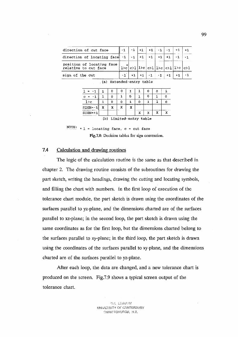
99

direction of cut face -1 -1 +1 +1 I -1 -1 +1 +1

direction of locating face -1 -1 +1 +1 +1 +1 -1 -1

position of locating ~ relative to cut face l>c c>l l>c c>l l>c c>l l>c c>l

sign of the cut -1 +1 +1 -1 -1 +1 +1 -1

(a) Extended-entry table

1

o o

x (b) Limited-entry table

NOTE: *1 1 t' f tf = oca 1ng ace, C 5 CU ace

Fig. 7.8: Decision tables for sign convention.

7.4 Calculation and drawing routines

The logic of the calculation routine is the same as that described in

chapter 2. The drawing routine consists of the subroutines for drawing the

part sketch, writing the headings, drawing the cutting and locating symbols,

and filling the chart with numbers. In the first loop of execution of the

tolerance chart module, the part sketch is drawn using the coordinates of the

surfaces parallel to yz-plane, and the dimensions charted are of the surfaces

parallel to xz-plane; in the second loop, the part sketch is drawn using the

same coordinates as for the first loop, but the dimensions charted belong to

the surfaces parallel to xy-plane; in the third loop, the part sketch is drawn

using the coordinates of the surfaces parallel to xy-plane, and the dimensions

charted are of the surfaces parallel to yz-plane.

After each loop, the data are changed, and a new tolerance chart is

produced on the screen. Fig.7.9 shows a typical screen output of the

tolerance chart.

L;13FlAfW UNiVERSITY OF CANTERBURY

CHRISTCHURCH,

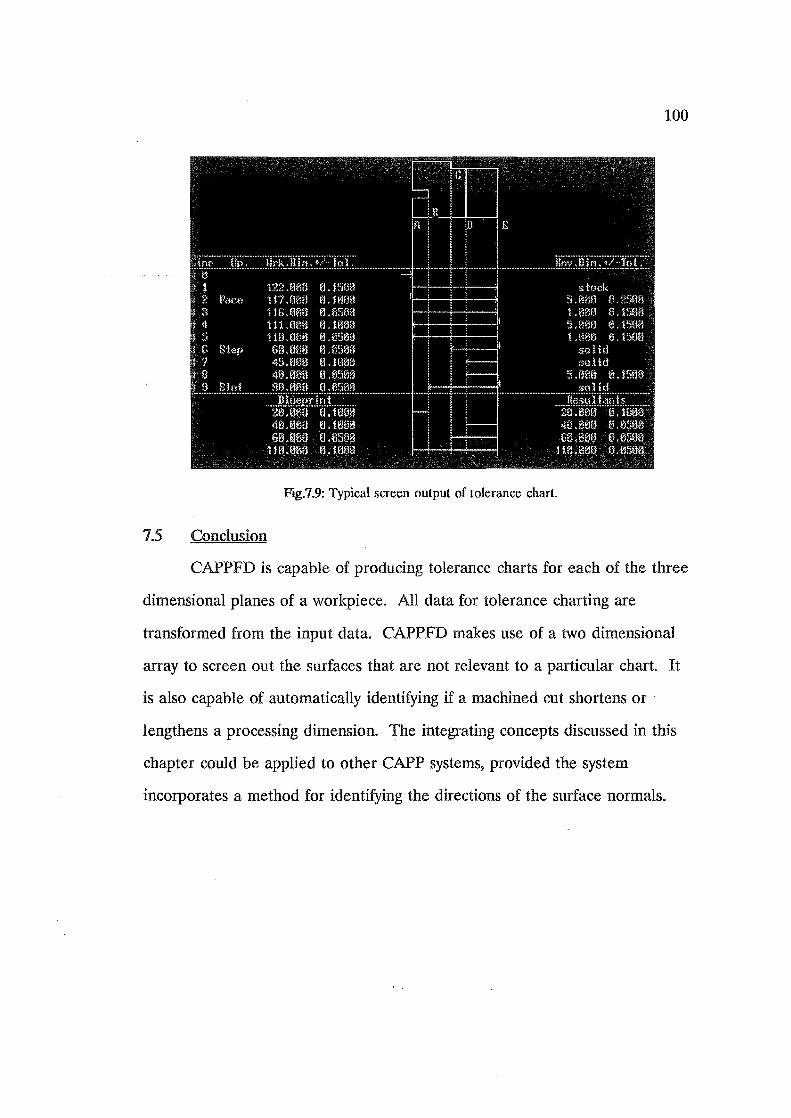
100

F.g.7.9: Typical screen output of tolerance chart.

7.5 Conclusion

CAPPFD is capable of producing tolerance charts for each of the three

dimensional planes of a workpiece. All data for tolerance charting are

transformed from the input data. CAPPFD makes use of a two dimensional

array to screen out the surfaces that are not relevant to a particular chart.

is also capable of automatically identifying if a machined cut shortens or .

lengthens a processing dimension. The integrating concepts discussed in this

chapter could be applied to other CAPP systems t provided the system

incorporates a method for identifying the directions of the surface normals.

101

. 8. RUNNING THE CAPPFD SYSTEM

. In this chapter guidelines for running the CAPPFD system are given.

The general steps of using the system are listed as follows:

(1) prepare the spatial representation data of the machined part,

(2) compile and link all the modules,

(3) execute the program,

( 4) enter (or edit) the production data,

(5) interact with the system to print the output on the line-printer.

These steps are demonstrated by the following two examples. In

Example 1 the production data are interactively input into the system through

a dialogue. Example 2 assumes the data are already stored in a data file, the

contents of this data file being given.

8.1 Example 1

(1) Model data file:

The specifications of the machined part are given in the drawing,

Fig.8.l. From these specifications the spatial matrix representation of the

part is developed (see Fig.(2) and stored in a data file. Fig.8.2 shows the

contents of this data file. The first line gives.the numbers of depths, rows,

and columns of the spatial representation. This is followed by the matrices

arranged in an increasing order of the depths.

10.00tO.OS 39.00

20.00 [

--110. 00

60.00't0.05 75.00

30.00 ~

-... ~ ~

- 40. 00

90.00

NOTE: ALL DIMENSIONS ARE IN MILLIMETRES 'V' ALL OVER

10.00 LINEAR TOLERANCES: + 0.10 EXCEPT STATED OTHERWISE MATERIAL: MILD STEEL (S7xl02x122 MM)

FJg.8.1 Drawing of a bracket.

(1) Starting up the system:

102

All modules are compiled and linked by a batch file, 'dp.bat'. This

produces an executable file, 'pfd.exe'. To run the system, simply type 'pfd', or

'pfd' followed by the name of the spatial representation file as follows: pfd

wm10.dat < cr> . Here the data file is wm10.dat.

(3) Data input:

The session for input of the production data starts with the screen

display as shown in Fig.8.3. When 'p' is entered, the screen in Fig.8.4 is

printed on the line-printer. (It should be noted that this command is also used

to dump any graphics screen to the printer.) This printout is used for

identifying the surface numbers of the part, which are required for data input.

CAPPFD then asks for a file name for storing the data. After this, the

dialogue for input of the production data starts.

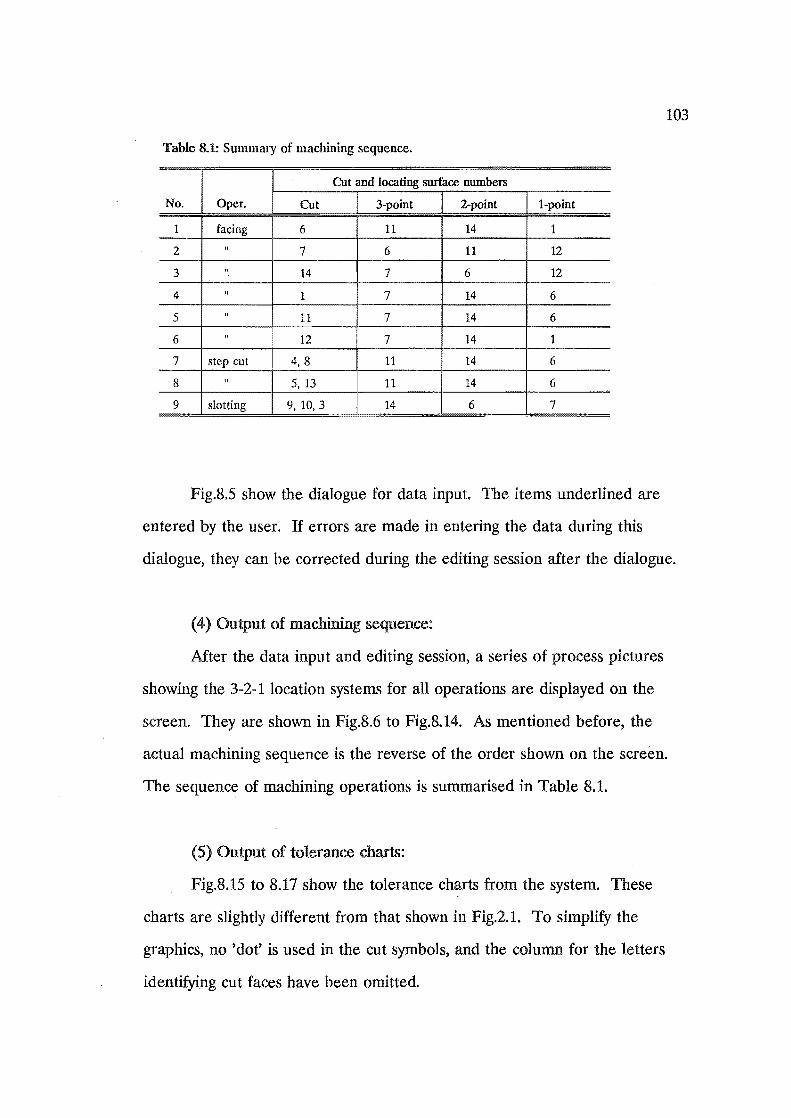
103

Table 8.1: Summary of machining sequence.

Cut and locating surface numbers

No. Oper. Cut 3-point 2-point I-point

1 facing 6 11 14 1

2 " 7 6 11 12

3 " 14 7 6 12

4 " 1 7 14 6

5 " 11 7 14 6

6 .. 12 7 14 1

7 step cut 4,8 11 14 6

8 " 5,13 11 14 6

9 slotting 9,10,3 14 6 7

Fig.8.5 show the dialogue for data input. The items underlined are

entered by the user. If errors are made in entering the data during this

dialogue, they can be corrected during the editing session after the dialogue.

(4) Output of machining sequence:

Mter the data input and editing session, a series of process pictures

showing the 3-2-1 location systems for all operations are displayed on the

screen. They are shown in Fig.8.6 to Fig.8.14. As mentioned before, the

actual machining sequence is the reverse of the order shown on the screen.

The sequence of machining operations is summarised in Table 8.1.

(5) Output of tolerance charts:

Fig.8.1S to 8.17 show the tolerance charts from the system. These

charts are slightly different from that shown in Fig.2.1. To simplify the

graphics, no 'dot' is used in the cut symbols, and the column for the letters

identifying cut faces have been omitted.

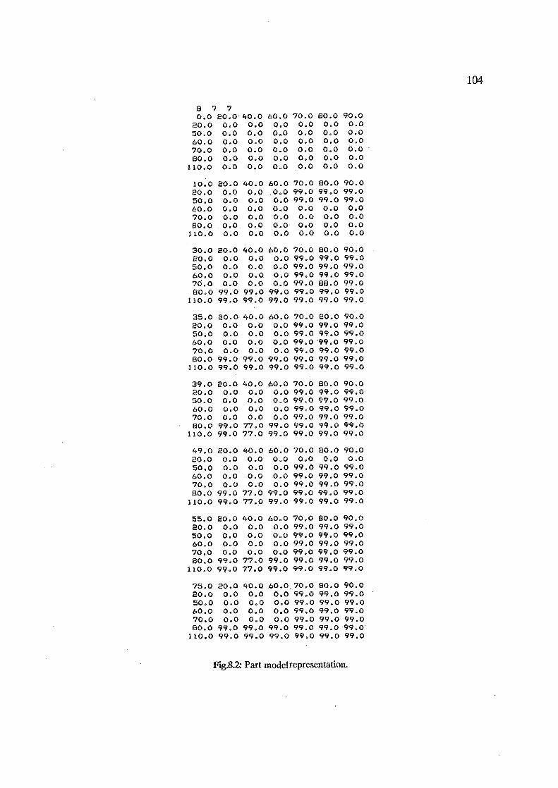
8 7 7 0.0 20.0'40.0 60.0 70.0 80.0 90.0

20.0 0.0 0.0 0.0 0.0 0.0 0.0 50.0 0.0 0.0 0.0 0.0 0.0 0.0 60.0 0.0 0.0 0.0 0.0 0.0 0.0 70.0 0.0 0.0 0.0 0.0 0.0 0.0 80.0 0.0 0.0 0.0 0,0 0.0 0.0

110.0 0.0 0,0 0.0 0.0 0.0 0.0

10.0 20.0 40.0 60.0 70.0 80.0 90.0 20.0 0.0 0.0 0.0 99.0 99.0 99.0 50.0 0.0 0.0 0.0 99.0 99.0 99.0 60.0 0.0 0.0 0.0 0.0 0.0 0.0 70.0 0.0 0.0 0.0 0.0 0.0 0.0 80.0 0.0. 0.0 0.0 0.0 0.0 0.0

110.0 0.0 0.0 0.0 0.0 0.0 0.0

30.0 20.0 40.0 60.0 70.0 80.0 90.0 20.0 0.0 0.0 0.0 99.0 99.0 99.0 50.0 0.0 P.o 0.0 99.0 99.0 99.0 60.0 0.0 0.0 0.0 99.0 99.0 99.0 70.0 0.0 0.0 0.0 99.0 88.0 99.0 80.0 99.0 99.0 99.0 99.0 99.0 99.0

110.0 99.0 99.0 99.0 99.0 99.0 99.0

35.0 20.0 40.0 60.0 70.0 80.0 90.0 eo.O 0.0 0.0 0.0 99.0 99.0 99.0 50.0 0.0 0.0 0.0 99.0 99.0 99.0 60.0 0.0 0.0 0.0 99.0'99.0 99.0 70.0 0.0 0.0 0.0 99.0 99.0 99.0 80.0 99.0 99.0 99.0 99.0 99.0 99.0

uo.O 99.0 99.0 99.0 99.0 99.0 99.0

39.0 20.0 40.0 60.0 70.0 80.0 90.0 20.0 0.0 0.0 0.0 99.0 99.0 99.0 50.0 0.0 0.0 0.0 99.0 99.0 99.0 60.0 0.0 0.0 0.0 99.0 99.0 99.0 70.0 0.0 0.0 0.0 99.0 99.0 99.0 80.0 99.0 77.0 99.0 99.0 99.0 99.0

110.0 99.0 77.0 99.0 99.0 99.0 99.0

49.0 20.0 40.0 60.0 70.0 80.0 90.0 20.0 0.0 0.0 0.0 0.0 0.0 0.0 50.0 0.0 0.0 0.0 99.0 99.0 99.0 60.0 0.0 0.0 0.0 99.0 99.0 99.0 70.0 0.0 0.0 0.0 99.0 99.0 99.0 80.0 99.0 77.0 99.0 99.0 99.0 99.0

110.0 99.0 77.0 99.0 99.0 99.0 99.0

55.0 eo.o 40.0 60.0 70.0 80.0 90.0 eo.o 0.0 0.0 0.0 99.0 99.0 99.0 50.0 0.0 0.0 0.0 99.0 99.0 99.0 60.0 0.0 0.0 0.0 99.0 99.0 99.0 70.0 0.0 0.0 0.0 99.0 99.0 99.0 80.0 99.0 77.0 99.0 99.0 99.0 99.0

110.0 99.0 77.0 99.0 99.0 99.0 99.0

75.0 20 • .0 40.0 ,60.0,70.0 80.0 90.0 20.0 0.0 0.0 0.0 99.0 99.0 99.0 50.0 0.0 0.0 0.0 99.0 99.0 99.0 60.0 0.0 0.0 0.0 99.0 99.0 99.0 70.0 0.0 0.0 0.0 99.0 99.0 99.0 80.0 99.0 99.0 99.0 99.0 99.099.0

110.0 99.0 99.0 99.0 99.0 99.0 99.0

FJg.8.2: Part model representation.

104

105

n \ ,,, 1

~ r-",

4 ""~ ... 13 5

S 14 12

\ ta9 ? Type:'"

'p' to print this screen for an input of production data. or

11 ~ <GN> it' data is already in a file.

FJg.83: The first screen display of the part.

., n 1 ,~

~ r-",

4 ........... 13 5

S 14 12

\ \ \

ta9 ?

Surface nUMbers on part

11 \. B

FJg.8.4: Surface numbers on the part.

Enter file nmme for storing data: ~rod.dat

Number of stock dimensions (type 0 if no stockdimemsion): 3 Enter stock dimensions:-# 1 :.- s't;k. dim. from:--L

stk. dim. tCI : 2..... 't;cllerance(mm): 0.15

# 2:- stk. dim. f)-om: 2. stk. dim. tCI : ii tCllerance(mm): 0.15

# 3:- stk. dim. f)-clm: 12 st~(. dim. tCI : 1!t t CI I e)- clnC e ( mm): 0 • 15

Numb en- clf drawing dimensiclns: 10 Enter drawing dimensions:-# 1:- dwg. dim. from: 2.

dwg. dim. tCI : 5L dimensiccn(mm): 39.00 tClle)-ance(mm): 0.10

# 2:- dwg. dim. from: ~ dwg. dim. tCI : 10 dimension(mm): 10.00 tCllerance(mm): 0.05

# 3:- dwg. dim. frclm: 2 dwg. dim. tCI : 3 dimensicln(mm): 20.00 tCllerance(mm): 0.10

4t 4:- dwg. dim. f)-clm: ~ dVJg. dim. tCI : 5 dimensiccn(mm): 40.00 tCllerance(mm): 0.10

4t 5:- dwg. dim. frc,m:.E... dwg. dim. to : ~ dimensic,n(mm): 60.00 tCllerance(mm) = 0.05

# 6:- dwg. dim. from: ~ dwg. dim. tCI :....L dimension(mm): 110.00 tCllerance(mm): 0.10

4t 7:- c!;.oJg. dim. frclm: ~ dwg. dim. to :.2 dimensicln(mm): 10.00 tClle)-ance(mm): 0.10

# 8:- dWfd , dim. frclm: 1.1 d~~g. dim. tCI :.2 d i mens i cln ( mm): 75.00 tClle:·rance(mm): 0.10

#_ 9:- dVJg. dim. from: ~ dwg. dim. tCI : 14-d imensi cln( mm): 30.00 tCllerance(mm): 0.10

# 10:- dwg. dim, from: 12 dwg. dim. tel: 14 dimensiccn(mm): 90.00 tolcrance(mm): 0.10

FJg.85: Dialogue for data input.

106

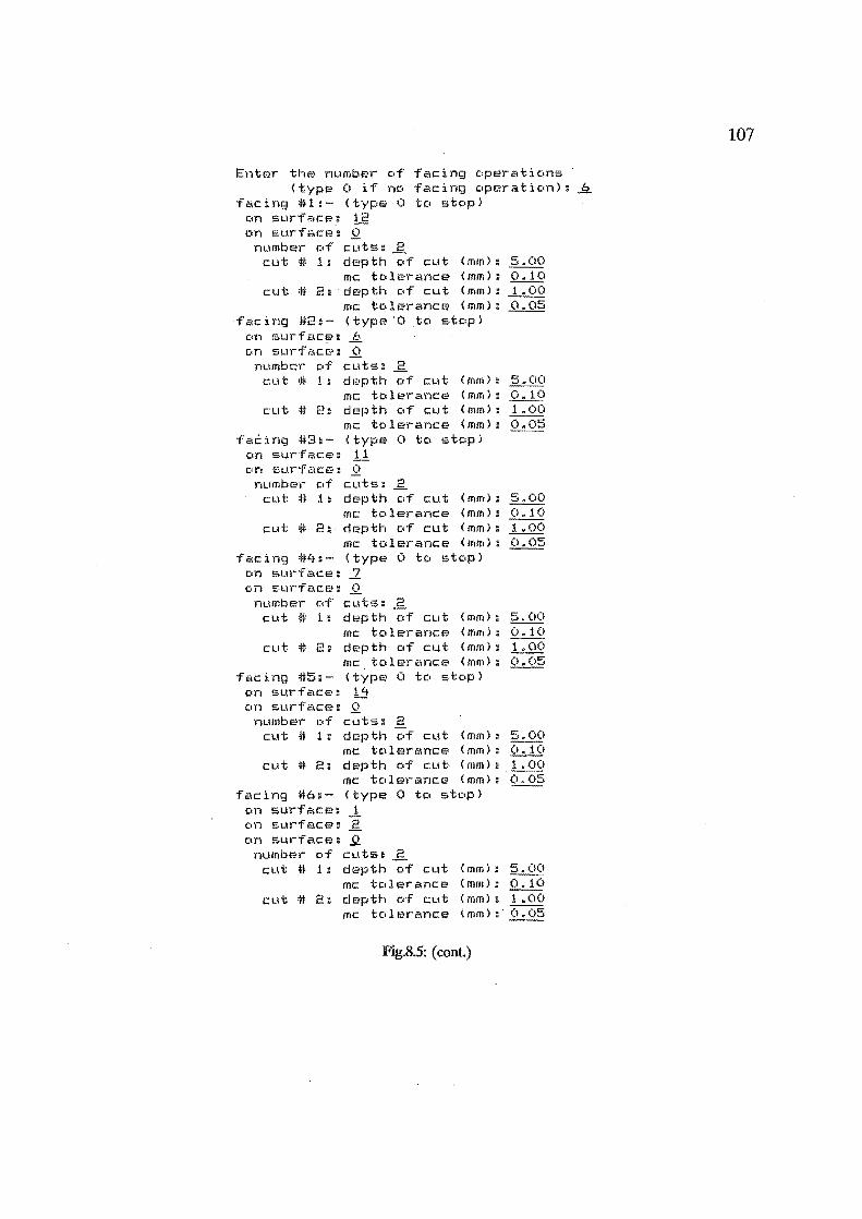
Enter the number of facing operations (type 0 if nc. facing c.peraticln): S

i"acing #1: (type 0 tel stop) em sLlrface: H'? cln Sl.lrf".ce: Q

nLlmber e.f cuts: ..£. cut # 1: depth e.f cut (mm): 5.00

mc te.lerance (mm); 0.10 cut # 2- depth elf cut (mm): 1.00

mc tolerance (mm): 0.05 facing #2:- (type 0 to stop)

e.n sLlrf"lce: numbc'l" elf CLltS: ...£ cut # 1: depth of cut (rom):

me tc.lel-ance (mm): 0.10 cut # 2: depth of cut (mm):

mc tolerance (mm): fa~ing #3:- (type 0 to stop)

c·n sl.lr"face: 1.1 e,n !;;·urface: Q

numbe',- elf CLltS: ..E.. cut # 1: depth of cut (mm) :

me tellerance (mm) : cut # 2= depth of cut (mm) :

(mm) : mc tell erance facing #4:- (type 0 to stop)

on sl.wf'::lce: .2 eln :;.Ln-face: .Q

nllmber elf ClltS:

5.00 0.10 1.00 0.05

cut # 1: depth elf cut (mm): 5.00 mc tellerance (rom): 0.10

Cllt 410 2: depth of cut (rom): 1.00 me tolerance (mm);

facing #5:- (type 0 to stop) e.n surf'::,I:e: 14 e.1'1 E;;llrface: Q

number Df cuts: 2 cut 4t 1: depth c.f cut (mm): 5.00

me tc:.lerance (mm): 0.10 cut # 2: depth elf cut· (mm): 1.00

mc te.lel-anee (mm): 0.05 facing #6:- (type 0 to stop)

em surfF.lce: 1 e.n surface: .£. on sUI-face: Q

numbel- of cuts: CLlt # 1: depth of cut (mm): 5.00

mc t c. 1 er a nc e ( mm): O. 10 cut # 2: depth Df cut (mm): 1.00

mc tolerance (mm): 0.05

FJg.85: (cont.)

107

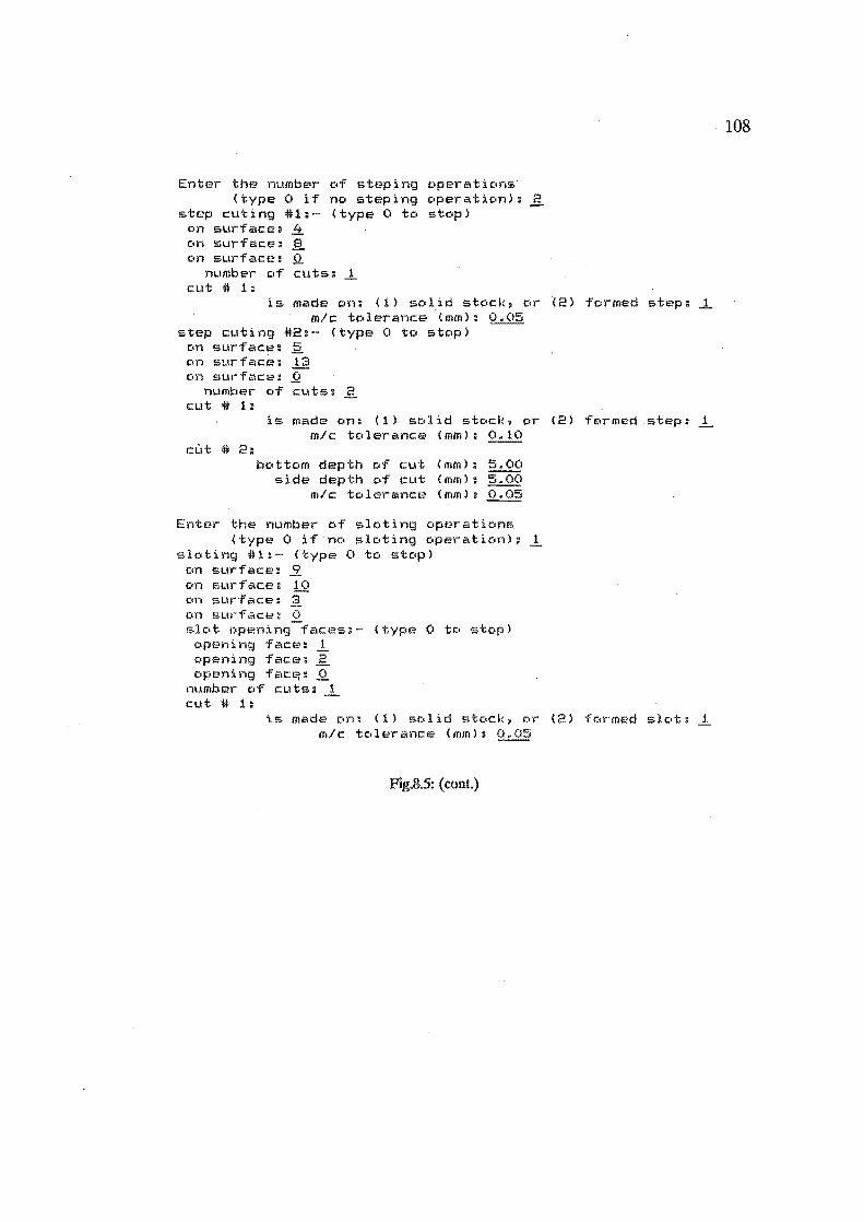
Enter the number of steping operations (type 0 if no steping operation): 2

step cuting #1:- (type 0 to stop) eln surfclcen i±. (In surface: .§. c:,n sLlrface: Q

nLlmber clf cuts: -1-cut # 1:

is made on: (1) sCllid stclcl(, clr '(2) formed step:..1. m/c tDlerance (mm):

step cuting #2:- (type 0 to stop) (In surface: 5 eln sLlrfC'.ce: 13 ell"') SLIl-f<.lce: .Q

number of cuts: 2 cut # 1:

is made cln: (1) sCllid stclcI(, clr (2) fClrmed step:...L mlc tDlerance (mm):

Cl.lt # 2: bottom depth of cut (mm): 5.00

side depth clf cut (mm): 5.00 m/c tCllerance (mm): 0.05

Enter the number of sloting operations (type 0 if no slDting DperatiDn): 1

slcltil'g #1: (type (I tD steip) cm surface: 9 CIl") sLlrface: 10 cln sur'f ace: £.. on surface: (I

slclt opl~ning-f",ces:- (type (I tCI stop) elpening face: ..1 elpening face: .£ clpeni ng facep Q

l,umber clf cuts: cut # 1:

is made on: (1) solid stock, Dr (2) formed slot: -1-mlc tolerance (mm):

F'Ig.85: (cont.)

108

t;>

..

\ 11

t A

to

it:

\ 11

\ \ \

ta9

A

&

.. \ " 'I

.l>\ 1

-", 4

>'5

S

\

?

a

Feature being nachined: slot: 9 16 3

FJg.8.6: Process picture for cutting slot(9, 10, 3).

~ &>.

13 ~ ... .t.

it' 12

Feature being nachined: step: 5 13

FJg.8.7: Process picture for cutting step (5, 13).

109

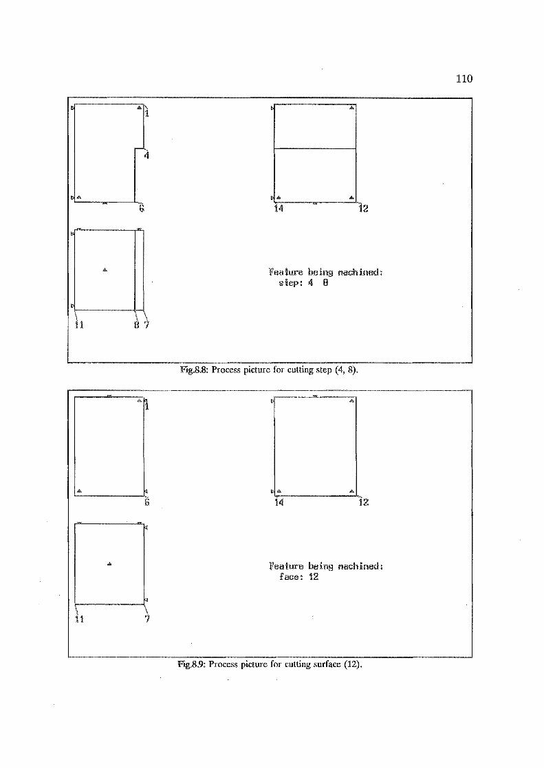
i ~ .lI.\ 1

c-, 4

I ~ .d1.

6

It:

...

Ir. \. \. \ 11 a 'I

i-------I,fl

~ ...

I'd. ... 14 12

Feature being nachined: step: 4 0

FIg.8.8: Process picture for cutting step (4, 8).

Feature being nachin8d~ face: 12

FIg.8.9: Process picture for cutting surface (12).

110

~---~~ \ "

14

Feature being Machined: face: 11

Ftg.8.l0: Process picture for cutting surface (11).

14

Feature being Machined: face: 1

Ftg.8.11: Process picture for cutting surface (1).

111

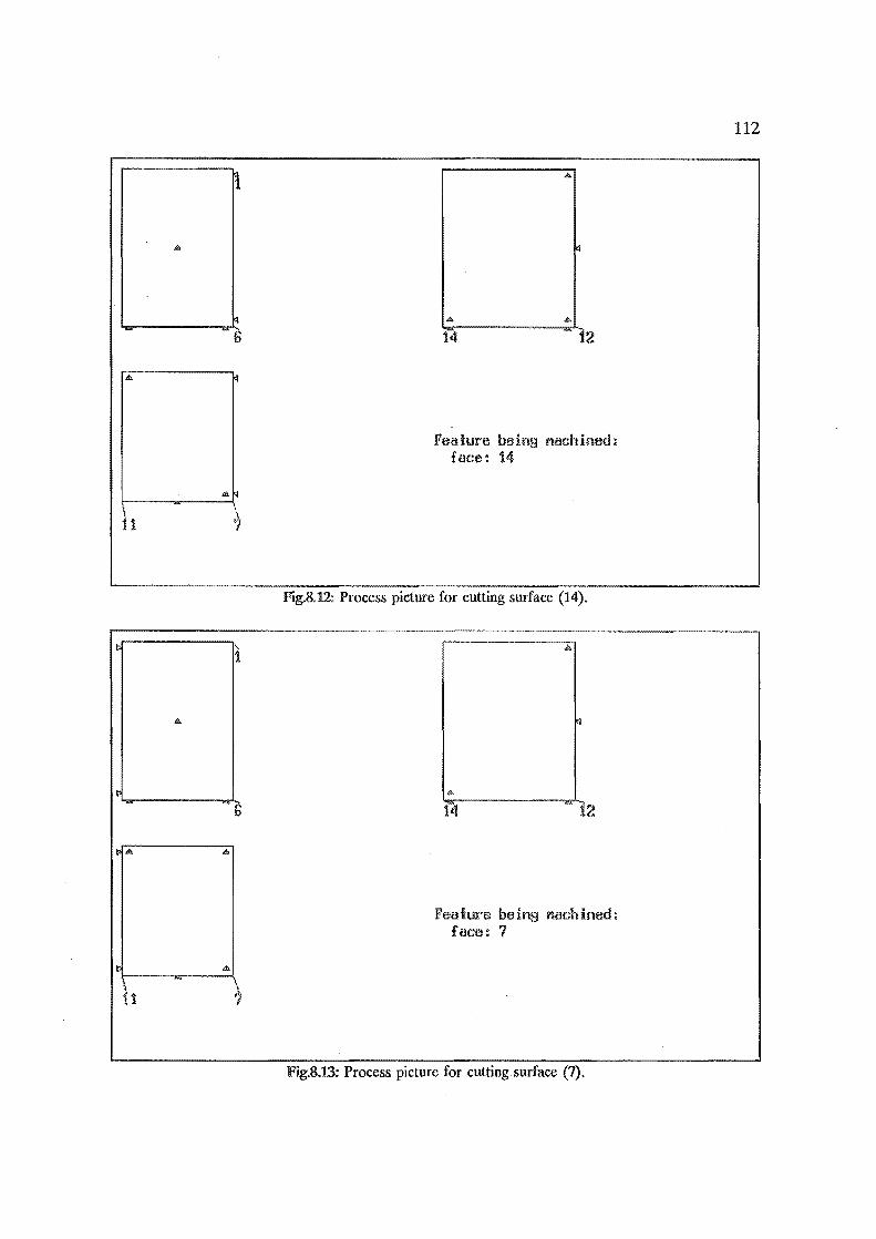
\ 'l

I~ 11

...

~

6

r. AI. .d>

t '" 11

I. 'l

14

Feature beinB Machined: face: 14

FIg-S.12: Process picture for cutting surface (14).

.Q.

~

'" 14 12

Feature beinB Machined: face: ?

FIg-S.n: Process picture for cutting surface (7).

112

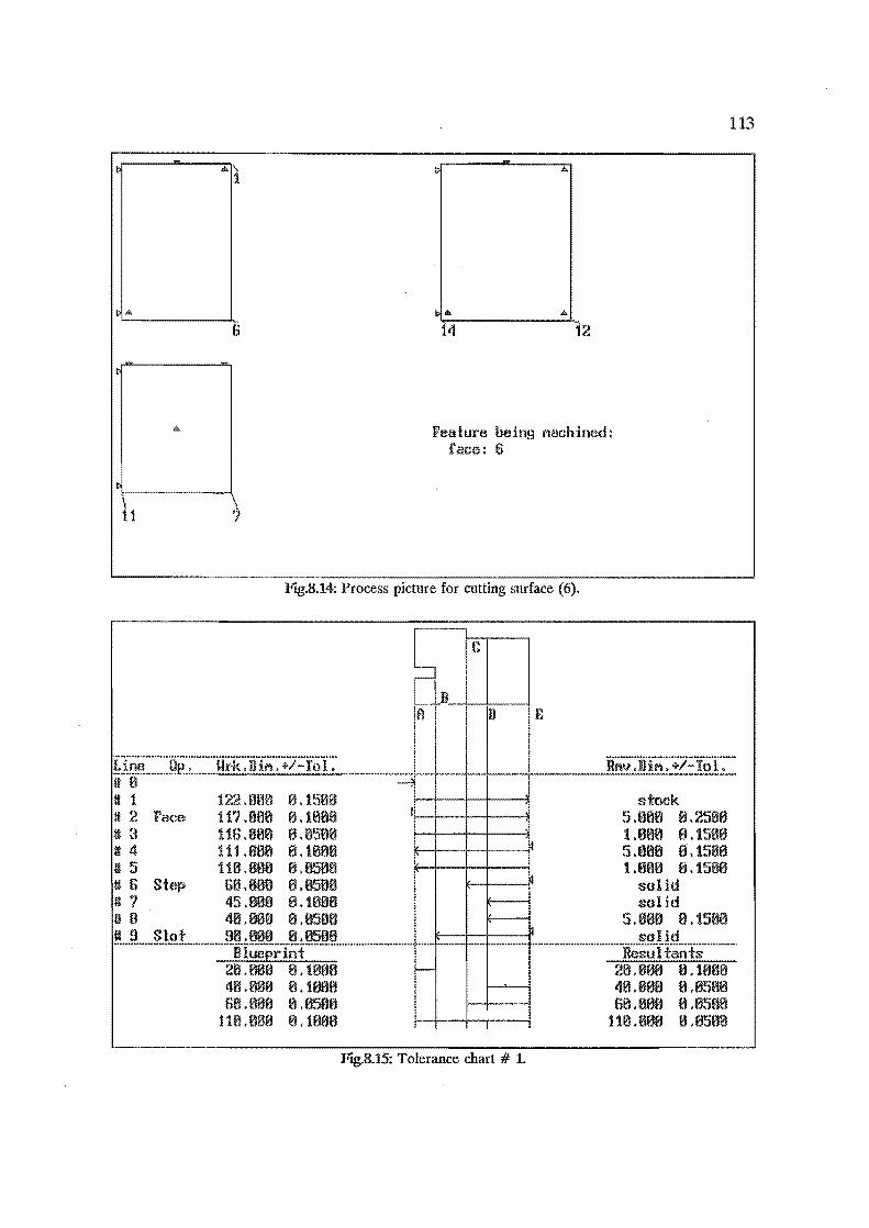
113

~ .!.\ i:' A 1

~ '" 11& '" 6 14 12

m Feature being nachined: face: 6

r,

\ 11 'I

FIg-8.14: Process picture for cutting surface (6).

FIg-8.lS: Tolerance chart # 1.

114

,.--- ,---

,D

~

B ~ L"in;;········op·:·········~x:k":·jli;;·:·+/::ToT:· nn;:;·:·jHM·:·+/.:·lo·r: .... H 8 ---i

H 1 B?m'1e 0, 15e~ stock H 2 J.'ace B2.mm 0.10e~ 5.r18e fj.25~0

H a Bt .aae 0. ~~50~ :I • fi00 f.I.15liB H 4 76.8a0 a.100f:l 5.000 fj • 15f:lf.l U S 75.880 8.850fl 1.800 B .iSflf.l

" 6 step 65.800 6.05Gfl sol id

" 7 Slot 39.600 6.05G6 sol id ~ ... ~ ................................ l~.:.~~~ ...... ~.:.~~.@JL ................................ ............. .. ........ sol id

....... ~J~~p..r~n.t.. ......... ·······································Resu"iTan"fs····· ...... 39.600 0.1086 f-- ····3·9·:·00S·····ij·:·05G'Er-HU:)00 e.050fj 18.008 0.05a8 1£1.0f..l0 0.1f:lf1tl 10.008 0.18m~ 75.0f..l0 0.1.00£1 '75.f:l0f.1 0.0500

FIg.8.l6: Tolerance chart # 2.

--

-

n

~ t nn;; ...... · .. Op·: .... ·· .. ·~ix:k·:·jji;;·: .. +;::ToT·:· nn;:;·:·fi·i;;·:·+/.:tor: .... H 8 -l

H 1 102 .~%WI 0, 150~ stock H 2 J.'ace 9?0ae 0.100~ I 5.008 f.I.25~0 H a 96.mm o .~~58~ 1.008 f.I.i5~B ti 4 91 .. mm a.i00f:l ~ 5.011l0 8.i5f:lf.l u S 913.880 8.850fl I 1.800 B .iSflf.l

" 6 Step 35.600 6.i00fl ~~ sol id U 7 313.600 8.0506 r--l 5.00B B.1566 ·········· .. ···· .. ··················:::::::ijJ~~P.:i:.!~:1:[::::::::: .............................. ..... u ............. ··· .. · .. ··j· .................... · .. · .......... ··ResuiTaf·l·{s .... · .. _·

38.600 0.10B6 ---l .. ··3fL00S ...... ij·:·05G·lr-98.600 0.1086

j 96.00B 8.05a8 ;

FIg-8.l1: Tolerance chart # 3.

115

. 8.2 Example 2

The part for machining in this example is a casting (Fig.8.18). Fig.8.19

shows the drawing of the finished part. Only slotting and facing operations

are required for this. The two slots are machined from solid cuts; that is the

slots are not formed as part of the casting.

38.00

! I 19.001 J

1

I 19.00

-I

I

I

(1) Data files:

82.00

I

134.00

75.00·

36.00

I r--

25.00 ~ ~ 25.00

139.00

ALL DIMENSIONS ARE IN MILLIMETRES TOLERANCES: +1.5 EXCEPT STATED

OTHERWISE

E}@.

FIg.S.1S: Drawing of a casting [76].

From the drawing of the finished part, the matrix spatial

representation is developed. The production data are worked out from both

drawings and a knowledge of the capability of the machine-tool.

Fig.8.20 shows how the principal axes are arranged on the part model.

Fig.8.21 shows the contents of the part model file.

Fig.8.22 shows the contents of the production data file.

The steps for starting up the system are the same as for Example 1.

50.00tO.05 44.00±O.05

12 . a a i---l----"

16.00tO.05

19.00±0.10 L-~~ __ ~ ______ ~

116

6.00±0.oa 25.00tJ..50

139. 00t3. 00

25.00tJ..50

127 00+0 30 - . -<'-T 12.00

I

1>

I

MATERIAL: CAST STEEL ALL DIMENSIONS ARE IN MILLIMETRES TOLERANCES: +5.00 EXCEPT STATED

OTHERWISE

FJg.8.19: Drawing of the machined part.

z x

FJg.8.20: Part with x-y-z axes.

(2) Output of machining sequence:

Fig.8.23 shows the first screen display. Fig.8.24 to 8.28 are the results

from the sequencing and locating routines. The summary of these results is

given in Table 8.2.

117

(3) Output of the tolerance charts:

Fig.8.29 to 8.33 show the tolerance charts. Note that if a screen is not

large enough to display the whole chart, another screen is used to display the

remainder of the chart, and they are shown as different figures.

. Table 82: Summary of machining sequence.

Olt and locating snrface numbers

No. Oper. Olt 3-point I-point

facing 10 7,8 11 23

2 1 . 10 11 22

3 19 10 11 22

4 slotting 6, 9, 18 10 11 22

5 13, 14, 5 10 19,20 22

8.3

The data for CAPPFD are of two types: one is concerned with the

geometric model representation of the part, and the other, with the cutting

conditions and the surfaces to be cut. The former is stored in a data file

prior to execution of the program. The latter can either be interactively input

into the system by the user or stored in a pre-prepared data file as for the

first type. The output from the system consists of a set of process pictures

showing the locating surfaces for all machining operations and a set of

tolerance charts analysing all the dimensions of the part. These results can be

used for tool designing purposes or as a basis for discussion with the product

designer.

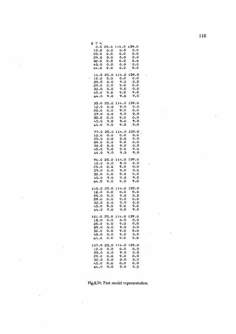
118

8 7 4 0.0 25.0 114.0 139.0

12.0 0.0 0.0 0.0 25.0 0.0 0.0 0.0 29.0 0.0 0.0 0.0 32.0 0.0 0.0 0.0 45.0 0.0 0.0 . 0.0 64.0 0.0 0.0 0.0

14.0 25.0 114.0 139.0 12.0 0.0 0.0 0.0 25.0 0.0 9.0 0.0 29.0 0.0 9.0 0.0 32.0 0.0 9.0 0.0 45.0 9.0 9.0 9.0 64.0 9.0 9.0 9.0

33.0 25.0 114.0 139.0 12.0 0.0 9.0 0.0 25.0 0.0 9.0 0.0 29.0 0.0 9.0 0.0 32.0 0.0 9.0 0.0 45.0 9.0 9.0 9.0 64.0 9.0 9.0 9.0

77.0 25.0 114.0 139.0 12.0 0.0 0.0 0.0 25.0 0.0 0.0 0.0 29.0 0.0 9.0 0.0 32.0 0.0 9.0 0.0 45.0 9.0 9.0 9.0 64.0 9.0 9.0 9.0

96.0 25.0 114.0 139.0 12.0 0.0 9.0 0.0 25.0 0.0 9.0 0;0 29.0 0.0 9.0 0.0 32.0 0.0 9.0 0.0 45.0 9.0 9.0 9.0 64.0 9.0 9.0 9.0

115.0 25.0 114.0 139.0 12.0 0.0 0.0 0.0 25.0 0.0 9.0 0.0 e9.0 0.0 9.0 0.0 32.0 0.0 9.0 0.0 45.0 9.0 9'.0 9.0 b4.0 9.0 9.0 9.0

121.0 25.0 114.0 139.0 12.0 0.0 0.0 0.0 25.0 0.0 9.0 0.0 29.0 0.0 9.0 0.0 32.0 0.0 9.0 0.0 45.0 0.0 9.0 0.0 b'I.O 0.0 9.0 0.0

127.0 25.0 114.0 139.0 12.0 0.0 0.0 0.0 25.0 0.0 9.0 0.0 29.0 0.0 9.0 0.0 32.0. 0.0 0.0 0.0 45.0 0.0 0.0 0.0 b4.0 0.0 9.0 0·9

Ftg.8.21: Part model representation.

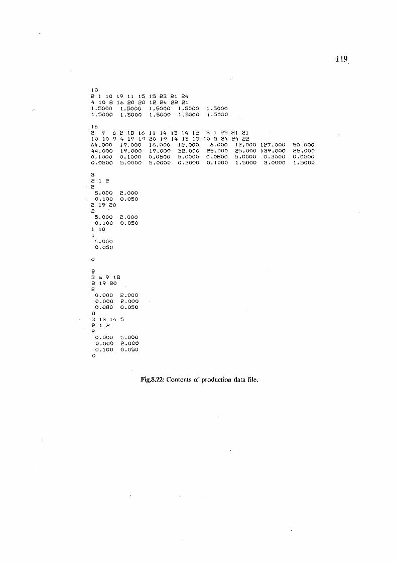
10' 2 1 10' 4 10' B 1.50'0'0' 1.50'0'0'

19 11 15 16 20' 20'

1.50'0'0' 1.50'0'0'

16 2 9 6 2 1B 16 10' 10' 9 4 19 19 M.cca 19.0'0'0' 44.0'0'0' 19.0'00' 0.10'0'0' 0'.10'0'0' 0'.0'50'0'

3 212 2

5.0'0'0'0'

5.0'0'0' 2.0'0'0' 0'.10'0' 0'.0'50'

2 19 20' 2

5.0'0'0 2.0'0'0 0'.10'0 0.050'

1 10' 1 4.0'0'0' 0'.050

o

2 3 6 9 18 2 19 20' 2

0'

0'.0'0'0' 0'.000' O.CBC

2.0'0'0' 2.00'0' 0'.050'

3 13 1'. 5 212 2

0.0'00' 0'.0'0'0 0'.10'0'

0'

5.00'0' 2.0'0'0 0'.0'50'

15 23 21 24 12 24 22 21 1.50'0'0' 1.50'0'0' 1.50'0'0 1.50'0'0'

11 14 13 14 12 20' 19 14 15 13 16.0'0'0' 12.0'0'0' 19.0'0'0 32.0'0'0' 0'.0'50'0' 5.0'0'0'0' 5.0'0'0'0' 0'.30'00'

1.50'0'0' 1.50'0'0'

B 1 23 10' 5 24

6.0'0'0' 25.0'00 C.CBCC 0' .10'0'0'

21 21 24 22

12.0'0'0' 25.0'0'0' 5.0'0'0'0' 1.50'0'0'

FIg.8.22: Contents of production data file.

119

127.0'0'0' 50.0'0'0' 139.00'0 25.0'0'0 0.30'0'0' 0'.0'50'0' 3.0'0'0'0' 1.50'0'0'

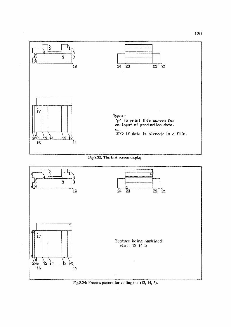
I \ 17

\ \1 " \ \ " .. ..

Type:'" 'p' to print this screen for an input of production data. or <CN> if data is already in a rile.

FIg.8.23: The first screen display.

24 23

Feature being tt8chined: slot: 13 14 5

FIg.8.24: Process picture for cutting slot (13, 14, 5).

120

I \ 17

\. \1 \ '.

[2

I AI

\

17

\. 1 \ '.

-~ 10

A~

\ '.

I L .. ... tl 24 23 22 21

Feature being Machined: sIal: 6 9 18

Hg..8.25: Process picture for cutting slot (6, 9, 18).

t··

1 10

£:1

\ '.

d ... b" 24 23 22 21

Feature being Machined: face: 19

Hg..8.26: Process picture for cutting surface (19).

121

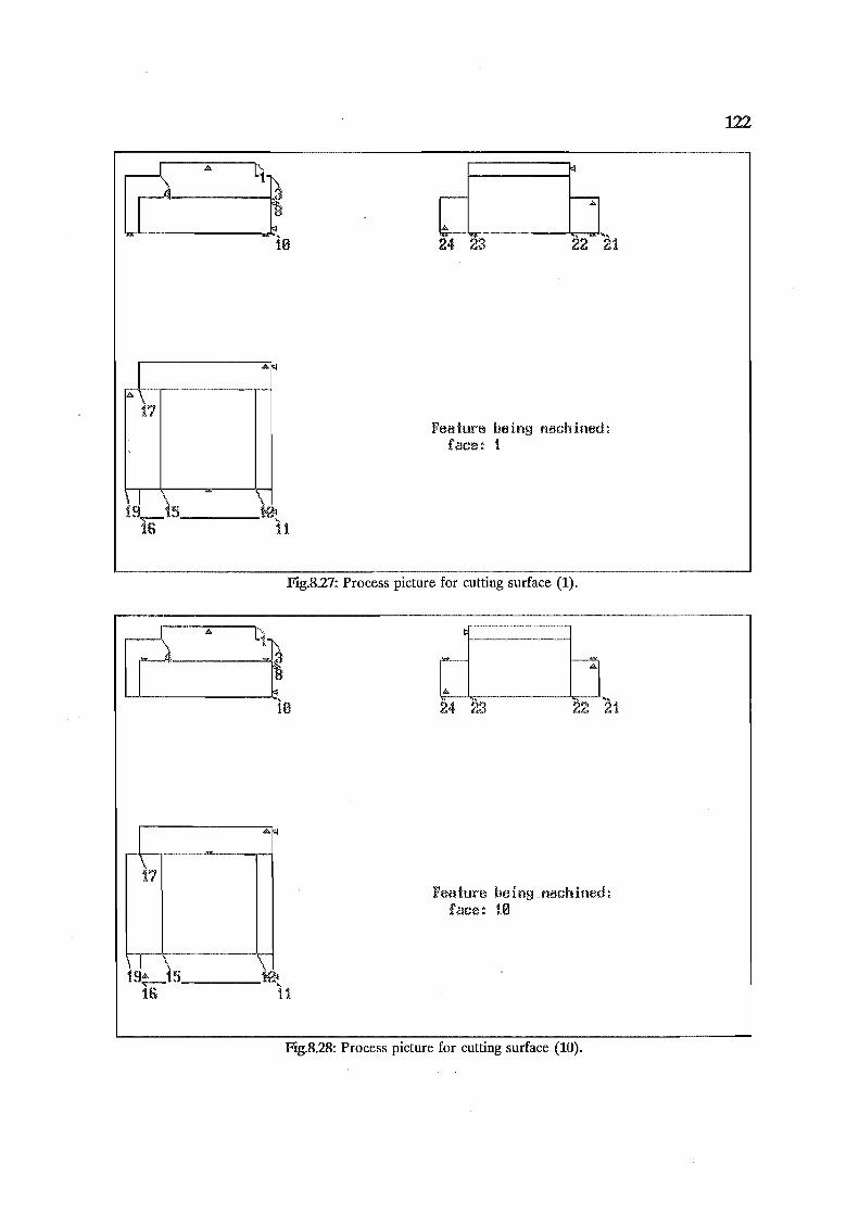
[2

I A\ ..

17

\. I >-..

C'-'

1 18

.... ~

>-..

d b" "" 24 23 22 21

Feature being Mw::hined: face: 1

Ftg.8.27: Process picture for cutting surface (1).

~ [-.

-~ 10

I .... ~

\ 17

\. I >- >-.. .. 19*-15 _____ 1!0I

16 11

d, b" 24 2" ..., 22 21

Feature being_Machined: face: 10

Ftg.8.28: Process picture for cutting surface (10).

122

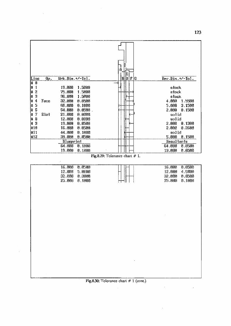
tI a It 4 Face It 5 II 6 II '1

" B " 9 ItO 1111 "12

19.fitltl 1.5mm '15.mm 1.5e00 m;; • am.~ l. seli0 32 . am~ a .858n 66.aaB e. 108n 6e) .0aB a . 058n . 21.0BB a .0888 12.080 8,0888 19.0mB 8.0588 16.08a 8,0588 4,1 • OfjfJ e . 1. fJ0ft ~:t9 .0fjfJ e .05.18

64 .0a13 0 , tfJa~:! 19.068 0,10aft

16.0f1e 0. 05fUl 12.0f1rJ 5.aaf:m 32.86a 8.3a09 25.B88 8,1809

FJg.8.29: Tolerance chart # 1.

FJg.8.30: Tolerance chart # 1 (cont.)

stock stock stock

4 .9aB 1. 55611 5.9a6 3.15611 2.006 0.15611

solid solid

2.mm 0.13£16 2.0a0 0,26£16

solid 5.0fJ8 0, 15m~ Resultants

64.6013 0.13590 19.611a B,859ft

16.013e 0 ,fJ5~18 12.aao 4 J.i090 32.88a tL 8S9a 25.8aO 8,1990

123

124

F"""""

-H~1D _ ..... c n-.. . 1 if) ~r u

I 1

I ! tInc···-···OE·: ... ······Urk"JHit·:·"+/=yor:· I Rnv]fiM. "+1-tor.-ti 0 jE-D 1 19,.188 1.5809 I 1 stock u 2 134.fU18 1.51:109 stock U ~l 3B.oa8 1.51:106

J I E-~ stock

U 4 82.080 1.50E:l8 I stock It 5 Face 129,mm 8.1£108 5.00a 1.6886 It G 127.880 6.350B I I ! 2.3aa a.1586 U '7 Slot 123.880 B.3B0B ~ I I ! solid U 8 121.880 8.e58B ! I 2.038 a,13BB M 9 52.0a0 8,1808 ! ~ solid D10 48.0a0 8,Um8 ! E--- solid ! fl11 58.Baa 8.0588 , 2.838 0.1586 ,

I fl1:? 4i1.8tiB 8 JiiJf'!:l ~ E--- 2.f:U:JB I!L~~BOO Blus2rint I I Resultants fi.Bti8 8.aSO!:l i ~ S.8aa a.1806

12.8118 5.HeOn , 12,800 3.B500 , Fig.831: Tolerance chart # 2.

12'] .Btia fL~jf:lm~ 12'J .a0e a.BS86 S8.8ti8 6.6508 58.60a B.aS86 44.8110 6.8588 r--- 44.0ea a.B586 1S.888 5.6e80 r- 19.aaa 3.1880 tS.8El8 5.0080 I--- '19.aaa 4.65813

F.tg.832: Tolerance chart # 2 (cont.)

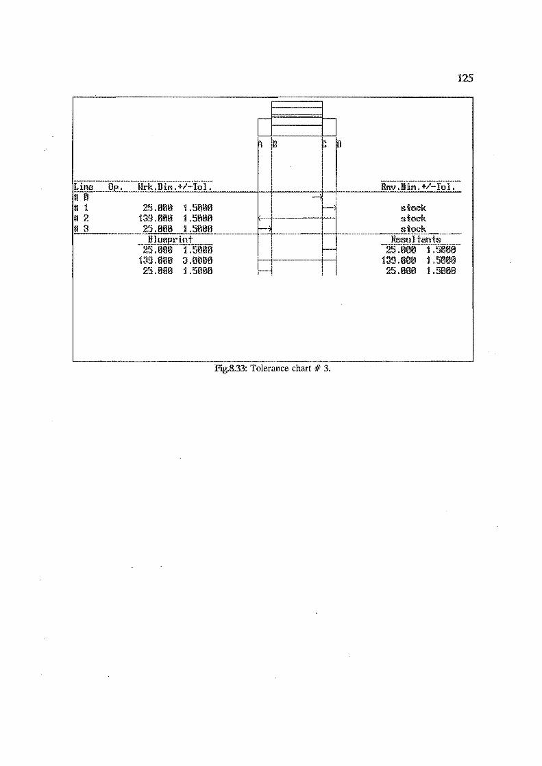
125

d h f'l IE b ~ I

I tlnc .... ··· .. {je·:·········ii~~:]H;;·:·:;/:foI·:· ii;:;v·:·O·ln·:·:;7.::·Io·r:···· ft 8

I -4i

ft 1 ~~5 .fifiO 1.5£100 h stock ft 2 1:l9.BfiO 1.5£100 ! stock U a 25.880 J .5e8a -J, stock

Blueeri.nt

I Resultants

25.880 1.5£lflH - 25.089 1.59£18 139.8130 :::1.00f1H j I

139.000 1, 500a 25.8130 1. 508H --! 25.008 l.saoa

FJg.833: Tolerance chart # 3.

126

·9. CONCLUSIONS AND RECOMMENDATIONS

This report puts forwards a new concept of computer-aided process

planning. Although the concept is commonly applied in manual process

planning, it has been neglected by the designers of most of the CAPP systems.

The CAPPFD system also incorporates a tolerance charting routine to check

the feasibility of the proposed processing sequence. This feature has not

previously been available in CAPP systems for prismatic parts. However, only

a start has been made, to prove the feasibility of incorporating these

techniques, and there is still a lot of work to be done to produce a fully

developed system. This is left for future research.

9.1 Conclusions

In generating the machining sequence, CAPPFD ensures dimensional

and geometric control over the workpiece. It demonstrates that it is feasible

to use the dimensional relationships as a basis for machining sequence

planning, and for locating the workpiece. Therefore, the general aim of this

research project has been achieved.

The logic for sequencing and locating the workpiece developed in

CAPPFD, can be adopted by other CAPP systems when the solid modeller is

fully developed.

With regards to the tolerance charting'technique, CAPPFD has

introduced a new method for tolerance stack calculations. This method may

be used in manual or computerised charting.

127

·9.2 Recommendations for future research

CAPPFD uses a spatial representation technique to model the

machined part in the computer. It is a simple method for solid modelling,

and it can represent the part geometry accurately only those containing the

edges parallel to the x, y or z axis. As a result, the system is confined to only

3 types of milling operation: facing, step cutting and slotting, which restricts

the system.

The system also has a limited capability for handling co~bined

features, particularly, when a step is on another step. When an error due to

this limitation occurs, the stock dimensions in the tolerance charts will not

agree with the actual dimensions. However, this can be picked up quickly by

the user, and changes can be made by modifying the depths of cut to be

consistent with the sequence. These shortcomings and others are subject for

future research. Some aspects of the future research are listed below:

(1) Other machined features: Features such as holes, closed and

open pockets should be included in the system. This could be

done by using an extended part model representation. It is

suggested that the sequence in which the new features are to be

processed must be pre-planned: in the same way as facing

before step cutting, step cutting before slotting in the present

work. The priority given will depend on the type of part family

and on the practical limi~ations in machining the features.

(2) Heat·treatment: Surface grinding normally follows case

hardening. At present, the tolerance chart module cannot

handle the case depth resulting from a grinding process. So

these two operations are not included in the system. With

further development of the tolerance chart technique, these

operations could be readily incorporated

128

(3) Tolerance chart calculations: Because the technique developed

for calculating the tolerance stacks is simple and suitable for

programming, it should be further developed to chart other

machined as well as non-machined features such as tapers,

radial surfaces, and hardened-case depth.

(4) Machining tolerance generation: An expert system could be

developed for generating the machining tolerances of the

prosessing operations involved. Some work, based on the

standard International Tolerance (IT) grades of average

machine-tool condition [33, 71], was done in this area, but it

does not take into account the skill and experience of the

machinist. This is the area where the expert system approach

should be applied.

(5) Mechanical control: An expert system should be developed for

designing a physical system. This may involve the use of other

engineering analysis package, such as the program for finite

element analysis; the data base of fixturing elements; and the

application program for designing a fixture. such as Ngoi's

system [52].

REFERENCES

1. Allen, K.D., 1987, An Introduction to Computer-Aided Process Planning, CIM, Fall.

129

2. Davies, RJ. and Darbyshire, LL., 1984, The Use of Expert Systems in Process lanning, Ann. CIRP, 33, 1.

3. Town, H.C., 1944, Jig and Fixture Practice, Paul Elek, London.

4. Gates, P., 1949, Jigs, Tools and Fixtures, 4th edition, Technical Press.

Kempster, M.H.A., 1974, An Introduction to Jig and Tool Design, 3th edition, Hodder and Stoughton, London.

6. Cole, C.B., 1946, Tool Design, American Technical Society Publisher.

7. Wilson, F.W.(ed), 1962, Handbook of Fixture Design, McGraw-Hill, New York.

8. Donaldson, c., LeCain, G.H., and Goold, V.c., 1973, Tool Design, Tata McGraw-Hill, New Delhi.

9. Henriksen, E.K., 1973, Jig and Fixture Design Manual, Industrial Press, New York.

10. Lander, L.C., 1944, The Principles of Process Planning, Flint., Mich.: General Motors Institute.

11. Doyle, L.E., 1950, Tool Engineering: Analysis and Procedure, Englewood Cliffs, N.J., Prentice-HalL

12. Eary, D.F., and Johnson, G.E., 1962, Process Engineering for Manufacturing, Englewood Cliffs, N.J., Prentice-Hall.

13. Wilson, F.W. and Harvey, P.D.(ed), 1963, Manufacturing Planning and Estimating Handbook, McGraw-Hill, New York.

14. Burbidge, J.L., 1975, The Introduction, to Group Technology, Heinemann.

15. Hayden, R.D., 1979, Computer Assisted Process Planning and MIPLAN System, O.I.R. Inc., Waltham, Massachusetts.

16. Link, C.H., 1976, CAPP-CAM-I Automated Process Planning system, 3th Numerical Control Society Technical Conference Proceedings,

Cincinnati, p.401.

17. Tulkoff, J, 1981, Lockheed's GENPLAN, 18th Numerical Control Society Technical Conference Proceedings, Dallas, Texas, p. 417.

130

18. Wang, H.P. and Wysk, R.A., 1986, Application of Microcomputers in Automated Process Planning, J. Of Manufacturing Systems, Volume 5, No.2.

19. Chang, T.C. and Wysk, R.A, 1983, CAD/Generative Process Planning with TIPPS, J. of Manufacturing Systems, Volume 2, No.2.

20. Sack, C.F.,Jr., 1982, Computer Managed Process Planning-A Bridge Between CAD and CAM, AUTOFACf 4 Conference Proceedings, Nov.30-Dec.2, Philadelphia, Pennsylvania.

21. Vogel, S.A. and Adlard, E.J., 1981, The AUTOPLAN process planning system, Numerical Control Society Proceedings, 18th Annual Meeting Technical conference, Dallas, Texas.

22. Eskicioglu, H and Davies, B.J., 1981, An Interactive Process Planning System for Prismatic Parts (ICAPP), Int. J. of Tool Des. Res., Vo1.21, No.3/4.

23. Descotte, Y. and Latombe, J.c., 1981, 'GARI: a problem solver that plans how to machine mechanical parts', Pro. of 17th International Joint Conference of Artificial Intelligence, Vancouver, B.C., Canada.

24. Darbyshire,!. L., and Davies, BJ., 1984, EXAP: An Expert Systems' Approach to Recursive Process Planning, 16th CIRP International Seminar on Manufacturing Systems, Tokyo, 13-14 July.

25. Iwata, K., and Sugimura, N., 1984, A Knowledge Based Computer Aided Process Planning system for Machine Parts, 16th CIRP International Seminar on Manufacturing Systems, Tokyo, 13-14 July.

26. Erve, A.H., and Kals, H.J.J., 1986, EXPLANE, a knowledge-base driven process planning expert system, International Conference on Computer-Aided Production Engineering, Edinburgh, April.

27. Mantyla, M, 1988, Feature-Based Product Modelling for Process Planning, 2nd Toyota Conference, Aichi, Japan, 2-5 October.

28. Biegel, J.E., 1986, The Future Role of Expert Systems in Manufacturing, Computer and Industrial Engineering, Vol.l1, No. 1-4.

29. Willis, D., Donaldson, I.A., Ramage, A.D., Murray, J.L., and Williams,M.H., 1989, A knowledge-based system for process planning

based on solid modeller, Computer-Aided Engineering Journal, February.

30. Choi, B.K., and Barash, M.M., 1985, STOPP: an approach to CADCAM integration, CAD, 17(4).

131

31. Lee, B.H., Lim, B.S., Lim, Y.G., and Ong, B.L., 1989, Extraction of Technological Information from Feature Oriented Modelling System for Generative Computer Aided Process Planning, International Conference on Productivity, 7-9 September, Singapore.

32. Alting, L., and Zhang, H., 1989, Computer-Aided Process Planning: the-state-of-the-art survey, Int. J. Prod. Res., Vo1.27, No.4, pp. 553-585.

33. Farmer, L.E., and Harris, A.G., 1984, Change of Datum of the Dimensions on Engineering Design Drawings, Int. J. Mach. Des. Res., VoL 24; No.4, pp. 267-275.

34. Farmer, L.E., Gladman, C.A., 1986, Tolerance Technology- Computer­Based Analysis, Annals of the CIRP, VoL 35/1.

35. Wiell, R.D., 1986, Present Tendencies in Computer-Aided Process planning, Software of Discrete Manufacturing, Crestin and J.F. Mcwaters (ed), Elsevier Science Publishers B.V. (North-Holland), pp. 223-235.

36. Chang, T.C., and Wysk, R.A., 1985, An Introduction to Automatic Process Planning Systems, Prentice-Hall International.

37. Joseph, A.T., and Davies, B.J., 1990, Knowledge based process planning system for turned components, Int. Adv. Manuf. Technol., 5:52-56.

38. Gandhi,M.V., and Thompson, B.S., 1984, Phase-change fixturing for FMS, Manufacturing Engineering, December.

39. Cutkosky, M.R., Eurokawa, E., and Wright, P.K., 1982, Programmable Comformable Clamps, AUTOFACT Conference Proceedings, SME, Dearbon, Michican, pp. 11.51-11.58.

40. Drake, T.R., 1985, The Computer-Aided of Production Tooling, Proceedings of the 1st National Conference on Production Research: Advances in Manufacturing Technology, Nottingham, UK, pp. 299-305.

41. Berry, D.C., 1982, Application of CAD\CAM to Fixture Design, National Machine Tool Builders' Association, IMTS-82 Technical Conference, September 8-17, pp. 43-66.

. 42. Miller, A.S., and Hannam, R.G., 1985, Computer aided design using a knowledge base approach and its application to design of jigs and fixtures, Proc. Instn. Engrs. Vol. 199, No. B4, pp. 227-234.

43. Nee, A.Y.C., Bhattacharyya, N., and Poo, AN., 1985, A Knowledge-Based CAD of Jigs and Fixtures, Tech. Paper No .

. TE 85-902, Society of Manufacturing Engineers, USA.

44. Anglert, PJ., and Wright, P.K.,1986, Applications of Artificial Intelligence and the Design of Fixtures for Automated Manufacturing, IEEE, pp. 345-351.

45. Lim, B.S., and Knight, J.A.G., 1986, Holdex-Holding Device Expert System. Proceedings of the First International Conference on the Applications of Artificial Intelligence in Engineering Problems, Southampton, UK, Vol.1, pp. 483-501.

46. Pham, D.T., Natgh, MJ., and Lazaro, AS., 1989, A Knowledge­Based Jig-And-Fixture Designers' Assistant, Int. J. Adv. Manuf. Technol., 4:26-45.

47. Pham, D.T., and Lazaro, A.S., 1990, AUTO FIX-An Expert CAD System for Jigs and Fixtures, Int. J. Mach. Tools. Des. Res., Vo1.30, No.3, pp. 403-411.

48. Davishi, A.R., and Gill, K.F., 1990, Expert system rules for fixture design, Int. J. Prod. Res., Vol. 28. No.lO, pp. 1901-1920.

49. Markus, A., Markusz, Farkas, J., and Filemon, J.,1984, Fixture Design Using Prolog: An Expert System, Robotics and Computer-Integrated Manufacturing, Vol.1, No.2, pp. 167-172.

50. Woodward, J.R., and Graham, D., 1983, Automatic Assembly and Inspection of Versatile Fixtures, Second International Conference on Flexible Manufacturing Systems, IFS(Conference), London, pp. 425-430.

51. Grippo, P.M., Gandhi, M.V., and Thompson, B.S., 1987, The Computer-Aided Design of Modular Fixturing Systems, Int. J. Adv. Manuf. Technol., 2(2), 75-88.

52. Ngoi, B.K.A., 1990, Computer-Aided Design of Modular Fixturing Assembly, PhD Thesis, University of Canterbury, New Zealand.

53. Chou, Y.c., Chandru, V., and Barash, M.M., 1987, A Mathematical Approach to Automatic Design Of Fixtures:

132

Analysis and Synthesis, ASME Winter Annual Meeting, Boston, PED. vol. 25, pp. 11-27.

54. Lee, J.D., and Haynes, L.S., 1987, Finite-Elements Analysis of Flexible Fixturing System, Transaction of the ASME, Vol.l09, May, pp. 134-139.

55. Halevi, G., and Wiell, R., 1985; Influence of Manufacturing Tolerances on Fixturing of machined Parts in Process Planning Systems, 1st Working Seminar-Papers-CIRP., pp.31-34.

56. Trappy, J.c., and Liu, C.R., 1990, A literature survey of fixture­design automation, Int. J. Adv. Manuf. TechnoL, 5:240-255.

57. Miller, J. R., 1989, Architechtural Issues in Solid Modelers, IEEE Computer Graphics and Applications, Sept., pp. 72-86.

58. Sakurai, H. and Gossard, D. c., 1990, Recognizing Shape Features in Solid Models, IEEE Computer Graphics and Applications, Sept., pp. 22-32.

59. Roy, U. and Lui, C.R., 1988, Feature-Based Representational Scheme of a Solid Modeler for Providing Dimensioning and Tolerancing Information, Robotics & Computer-Integrated Manufacturing, Vol. 4, No. 3/4, pp. 355-345.

60. Luby, S.c., Dixon, J.R., and Simmons, M.K., 1986, Creating and Using A Feature Database, Computers in Mechanical Engineering, November, pp. 25-33.

133

61. Gadzala, J.L., 1959, Dimensional Control in Precision Manufacturing, McGraw-Hill.

62. Johnson, AM., 1963, Tolerance Charts (Chapter 14 of Manufacturing Planning and Estimating Handbook: Edited by Wilson, F.W. and Harvey, P.D., McGraw-Hill.)

63. Wood, W.K., 1957, Tolerance Charts Aid Dimensioning for Machining, American Machinist, Dec. 30.

64. Anderson, J.F., Jr., 1956, Assembly Tolerance Charts: Save Time and Money, The Tool Engineer, Dec.

65. Irani, S.A., Mittal, R.O. & Lehtihet, E.A., 1989, Tolerance Chart Optimization, International Journal of Production Research, 26(2).

66. Marks, C.T., 1953, Tolerance Charts Control Production Machining, American Machinist, 97(5), pp. 114-116, March.

·67. Mooney, C.T., 1955, How to Adjust Tolerance Charts, The Tool Engineer, 35(4), pp. 75-81, October.

134

68. Johnson, A., 1954, Index Tolerance Chart Simplifies Production, The Tool Engineer, 32(2), pp. 53-62, February.

69. Wade, O.R., 1967, Tolerance Control in Design and Manufacturing, Industrial Press, New York.

70. Ahaluwalia, R.S. and Karolin, AV., 1984, CATC - a computer aided tolerance control system, Journal of Manufacturing System,3(2),pp.,153-160.

71. Xiaoqing, T. and Davies, 1988, BJ., Computer Aided Dimensional Planning, Int. J. of Prod. Res., 26(2), pp. 283-297.

72. Whybrew, K, Britton, G.A., Robinson, D.F. & Sermsuti-Anuwat, Y., 1990, A Graph-Theoretic Approach to Tolerance Charting, Int. 1. of Adv. Manuf. Technol., 5(2), pp.175-183.

73. Whybrew, K., Britton, G.A., Sermsuti-Anuwat, Y., 1990, An Algorithm for Tolerance Charting, International Conference on Auto Technology, Chulalongkorn University, Bangkok, Thailand, 12-14 November.

74. Whybrew, K., Britton, G.A., Serrnsuti-Anuwat, Y., 1991, Some Recent Developments in Tolerance Charting and Its Role in CIM, International Conference on Computer Integrated Manufacturing(ICCIM'91), Hyatt Regency Singapore, 30 Sept-1 Oct.

75. Doyle, L.E., 1950, Tool Engineering: Analysis & Procedure, Prentice­Hall.·

76. Chapman, W.A.J., 1955, Workshop Technology: Part 2, Edward Arnold.

77. Montalbano, M., 1974, Decision Tables, Science Research Associates, Inc.

78. McDaniel, H., 1968, An Introduction to Decision Logic Tables, Wiley & Sons.

79. McDaniel, H., 1970, Applications of Decision Tables, Brandon Systems Press.

APPENDIX A

GRAPH-THEORETIC APPROACH TO

TOLERANCE CHARTING

K Whybrew, G A Britton, D F Robinson and Y Sennsnti-annwat

University of Canterbury, Private Bag, Ham,

Christchurch, New Zealand

135

A major problem for manufacturing companies is the effective integration of design and

production. Tolerance charts provide one means of aiding this integration. Manually produced

chafts are time-consuming and have not been widely adopted. This paper presents an elegant

graph-theoretic approach to tolerance charting suitable for use with a microcomputer. The

approach has the potential to significantly reduce the amount of work required in charting, and so

it can be used by small companies as well as large ones.

Key words: Graph theory; Tolerance charts

1. Introduction

A tolerance chart is a graphical representation of a sequence of machining

operations on a workpiece. It shows the machined dimensions, the tolerance

and the amount of stock to be removed at each step in the sequence. The

main use of a tolerance chart is as a process planning tool to ensure that a

specific processing sequence is appropriate for producing a product of the

required finished dimensions, and that there is adequate metal to be removed

at each machining operation. It also provides an easy understood means for

136

, communication between the process planner and the designer. The chart can

disclose any problems concerned with tolerance control on the workpiece

before machining occurs, so that they can be analysed and the appropriate

remedial action taken.

Although the tolerance chart has been used for controlling dimensions

of machined parts since the early 1950s, the technique is practised only within

certain industries, for example the aircraft industry [1] and the automobile

industry [2]. The reluctance to a~cept the method comes from the complexity

of the chart itself: time and effort are required to learn and to practise the

technique. This obstacle has led to various methods being proposed to

simplify the charting. Among the well-known methods are those proposed by

Johnson [3], Mooney [4], Wade [5], and Gadzala [6]. Even with these

methods, however, the task is still time-consuming and error-prone.

It was not until 1982 that Sack [7] reported the use of the tolerance

chart in an automatic process planning system. This report opened up a new

and efficient way of computerised tolerance charting. Then Ahluwalia and

Karolin [8] used a minicomputer with a graphics routine to generate the

tolerance chart. Recently, Xiaoqing and Davies [9] have developed a

computer package for tolerance charting based on a matrix-tree-chain

method. These programs are limited to a minicomputer or mainframe

computer; there has not yet been any report of a similar application being

developed for use on a microcomputer.

The intention of this paper is to describe another tolerance-charting

approach, based on graph theory, which is appropriate for microcomputer

application. The approach is described by means of an example of a simple

tolerance chart in which a chosen sequence of machining operations cannot

meet the designer's specifications. The example is worked out manually and

137

. then the computer output for the particular example is presented.

2. Development of the Technique

The technique of tolerance charting developed here is based on the Urooted­

tree" method, which isa special kind of directed graph as described by

Robinson and Foulds [10]. The tolerance in Fig. 2 prepared for the

workpiece shown in Fig. 1, will be used as an example to illustrate the basic

ideas of the technique. This chart is slightly different from those of Johnson

[3], Wade [5] and Gadzala [6], in that no intermediate balance dimension is

shown between the working dimensions.

All the workpiece surfaces are identified by capital letters., The

surface pointed to by the arrowhead is the machined faced, and the surface

identified by a dot surrounded by a circle is the locating face. Since the

tolerance is concerned only with length dimensions, all diameter dimensions

are omitted from the chart. ( It should also be noted that operation 20 is not

listed in the chart because this operation does not have any effect on the

finished dimensions.)

The most important use of the chart is for finding the route from a cut

face to the original surface. Two approaches to the solution will be

presented: a. diagram and a tabulation method. Either approach can solve the

problem, but the diagram is more convenient for manual working and makes

the algorithm easier to understand.

Considering Fig. 2, the essence of this example can be stated as

follows:

Operation 10: face A of the stock is defined relative to locating surface D

Operation 30: face B is defined relative to surface D

Operation 40: face Al is defined relative to surface D (the numeric suffix is

138

.-------- fh 24.00±0.050

~'-..".',~

1- t"-"-.- f"<1--

l\ r/J 24.00::1:0.050 !6 45.00±0.050

r....'-.. '-.. '-.. '-.. "-

20.00::1:0.0 5 30.00± 0.050

60.00±0.010

FIg.l. Workpiece dimensions (in millimetres).

10 A 0.200

2 30 B 0.025 solid

3 40 Al 0.025 0.50 0.225

4 50 Dl lathe 60.20 0.025 0.50 0.050

5 60 C drill 30.60 0.025 29.60 solid

6 70 Cl lathe 30.10 0.025 0.50 0.050

7 80 0.10 0.030

8 90 0.10 0.010

resultant

20.00 0.080

30.00 0.060

60.00 0.005

FJg.2. Tolerance chart for the workpiece in Fig.!.

necessary to distinguish between the old and the newly machined surfaces)

Operation 50: face DI is defined relative to surface Al

Operation 60: face C is defined relative to surface Al

. Operation 70: face Cl is defined relative to surface Al

Operation 80: face A2 is defined relative to surface D 1

Operation 90: face D2 is defined relative to surface A2

139

This is summarized in Table 1 (which later becomes the first three columns of

. Table 2 in the tabulation approach). Diagrammatically, the machining

sequence can be represented by a "rooted-tree" graph, with the original

locating surface D (the "root") at the top, as shown in Fig. 3. In Fig. 3, each

link represents a machining operation with its associated working dimension,

and each node represents a machined and/or a locating surface; some nodes

are both a machined and a locating surface. The path from anyone node of

the tree to another can be easily picked out by inspection. The links in a

path define the machining operations, and determine the dimensions, relevant

to the two surface nodes. The distance, basic dimension and tolerance

between the two surfaces are the result of all machining operations that are

the links in the path. For example, the path from Cl to A2 is Cl Al Dl A2.

The tolerance of the distance between Cl and A2 is equal to the sum of the

tolerances of the machining operations in the path.

Table 1. Machined faces and locating surfaces.

Operation Machined face Locating face

10 A D 30 B D 40 AI D 50 DI At 60 C At 70 CI At 80 A2 Dt 90 D2 A2

140

F'tg3. Rooted-tree diagram.

In the tabulation method, the paths in the rooted tree are summarized

as shown in Table Under the "path" heading in the table, the path from

the new surface node to the root is listed. This is constructed by adding the

new face to the corresponding locating surface and the path from the locating

surface to the root, which has already been computed. In the "reversed path"

column, the path elements are reversed.

To find the path from any node to any node Y, the two reversed

paths are compared and the last node at which they agree is identified.

The path from X to Y is then given by the path from X to ("path X')

followed by the path from Z to Y ("reversed path Y"). For example:

1. Find the path from Cl to A2.

Reversed paths: Cl = D Al Cl

A2 = D Al Dl A2

Z = AI; hence the path from Cl to A2 is Cl Al D 1 A2.

2. Find the path from Al to A2.

Reversed paths: Al = D Al

A2 D Al Dl A2

141

Z = A1; hence the path is A1 D1 A2 (X occurs in the reversed path of

Y).

The links in a path are needed to find 'the tolerances. These links are

identified and listed against the machined surface at the end of the path, so

that they can be immediately extracted to add their tolerances together.

Table 2. Paths in rooted-tree diagram.

Operation New face Locating face Path Reversed path

10 A D AD DA 30 B D BD DB 40 Al D AID D Al 50 Dl Al DIAID DAI DI 60 C Al C AID DAI C 70 CI Al CIAID D Al CI 80 A2 DI A2 D1 Al D D Al DI A2 90 D2 A2 D2 A2 DI Al D D Al DI A2 D2

3. Applications

Fig. 4 summarises the procedure outlined above. First the basic data must be

prepared. This data includes the processing sequence, the tolerances for all

machining operations and the minimum amount of metal to be removed at

each machining cut. First a sketch of the workpiece, and then lines and

letters identifying all surfaces to be processed, are entered in the tolerance

chart. After this is done, the basic data and the charting symbols are entered

in the appropriate columns. At this stage, columns 5, 8 and the "resultant"

column are empty. These columns will contain the values that are to be

calculated.

Parts (b) and (e) of Fig. 4 are not parts of the tolerance chart; they are

shown to clarify the calculations. The table in Fig. 4(b) is similar to Table2,

except that two new columns have been added: column 13 records the links in

a path required for calculating a balance dimension, and column 14 is for the

line numbers corresponding to those links in column 13.

(a)

5

r­I

a / , ,,-

(b)

~ the sum of the tolerances of lines 1 and ) ,... 10 11 12

142

14

Line Op.no. Face HIe war ng cut , ~:~; path reversed path link for a balance dim.

no. aS1C face

D D D

10 A A D AD DA

)0 B B D BD DB

40 Al Al D AlD DAl

50 Dl Dl Al DIA1D DA1Dl

5 60 c. drill 30.60 C Al CAlD DA1C

70 Cl lathe 30.10 Cl A1 C1A1D DAlCl

7 80 A2 grind 60.10 A2 Dl A2DlAID DAIDIA2

90 D2 grind 60.00 D2 A2 D2A2D1AlD DAlDIA2D2

blueprint

20.00

30.00

~~~~jCtj~~~~', \ ' .... -

60.00 0.010

/

I I

I " ~the sum of the tolerances of

, lines 2,J,4 and 7

"-"­

Hnle ne no.

AD 1

AID 3

CAl 5

DIAl 4

A2Dl 7

A2Dl,DlA1,A1D,BD 7,4,3,2

CIA1,DIA1,A2Dl,D2A2 6,4,7,0

D2A2 8

, .... (e) )/ .... (d) 60.20 -....

(e) 'rooted tree'

.--+---1 m working dim. of cut 2

L-+--_ m : !~:~-!!~.2-(60.l-20» ~ Working dim. of aut 6

r---j.--l1Il : ~~:~ ~~60.l-(60-30»

.--+-----' ITl L...--+-.., [[)

FJg.4. Summary of the method of tolerance charting. (AU dimensions are given in millimetres;

squares in parts (c) and (d) denote line numbers.)

To calculate the tolerance on the metal removal of a cut, in column 8,

the tolerance of the cut is added to the sum of tolerances of the machining

operations corresponding to the line numbers in column 14; for example, the

tolerance of the metal removal in line 3 is

0.025 mm + 0.200 mm = 0.255 mm

This method is also applied to calculate the tolerances of all the resultants.

The basic working dimensions are worked out from the bottom

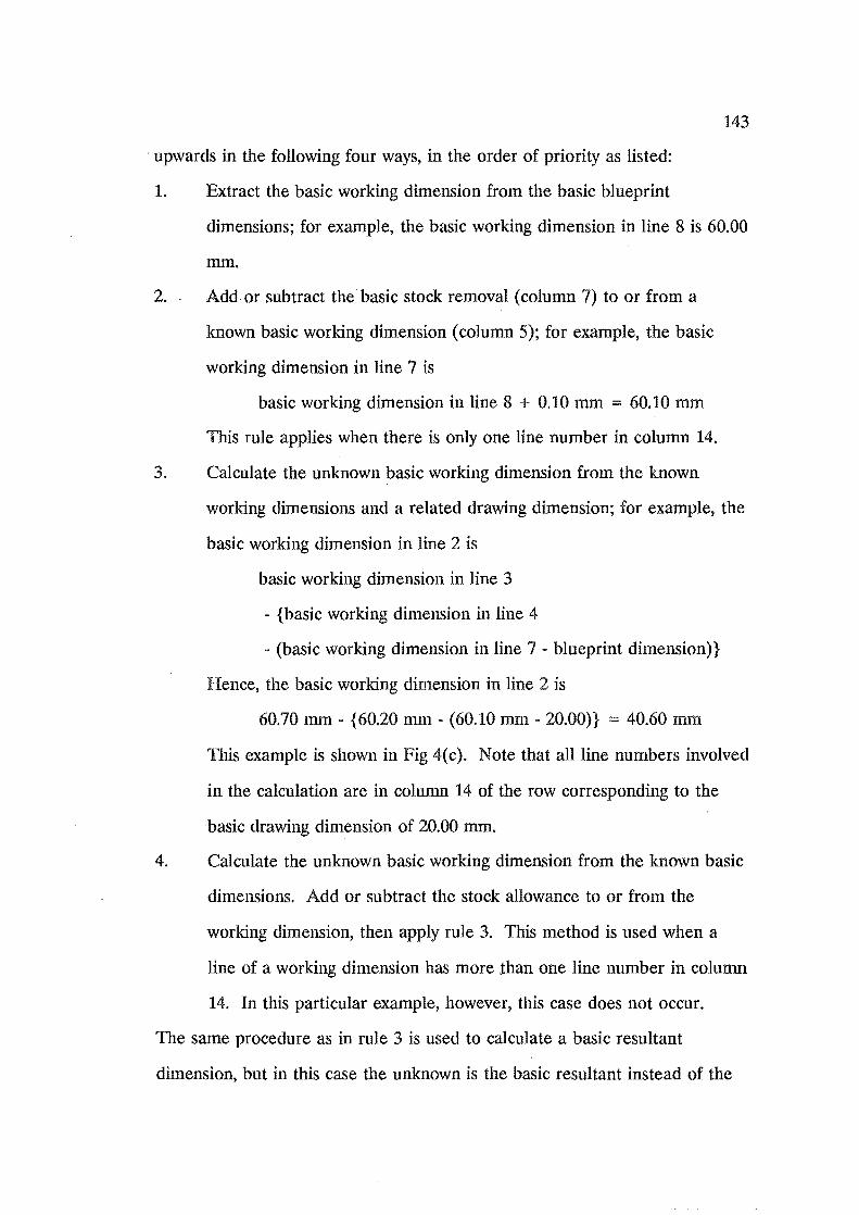
143

. upwards in the following four ways, in the order of priority as listed:

1. Extract the basic working dimension from the basic blueprint

dimensions; for example, the basic working dimension in line 8 is 60.00

rom.

2. Add or subtract the basic stock removal (column 7) to or from a

known basic working dimension (column 5); for example, the basic

working dimension in line 7 is

basic working dimension in line 8 + 0.10 rom = 60.10 rom

This rule applies when there is only one line number in column 14.

3. Calculate the unknown basic working dimension from the known

working dimensions and a related drawing dimension; for example, the

basic working dimension in line 2 is

basic working dimension in line 3

- {basic working dimension in line 4

(basic working dimension in line 7 - blueprint dimension)}

Hence, the basic working dimension in line 2 is

60.70 rom - {60.20 mm - (60.10 mm - 20.00)} := 40.60 rom

This example is shown in Fig 4(c). Note that all line numbers involved

in the calculation are in column 14 of the row corresponding to the

basic drawing dimension of 20.00 rom.

4. Calculate the unknown basic working dimension from the known basic

dimensions. Add or subtract the stock allowance to or from the

working dimension, then apply rule 3. This method is used when a

line of a working dimension has more than one line number in column

14. In this particular example, however, this case does not occur.

The same procedure as in rule 3 is used to calculate a basic resultant

dimension, but in this case the unknown is the basic resultant instead of the

144

. basic working dimension.

By comparing the blueprint and the resultant tolerances in Fig 4(a), it

can readily be seen that the chosen process sequence cannot produce a

workpiece to the required specifications. This is because the tolerances of the

resultant dimensions are greater than those of the corresponding blueprint

dimensions. These differences signify that modifications should be made to

either the type of machining operation, the tooling, or the machining

sequence. Column 14 in Fig. 4(b) provides the line numbers of the working

dimensions that relate to a finished product dimension. These line numbers

can be used as a basis for such modifications.

4. Computer-Aided Tolerance Charting

A computer program for the microcomputer, based on the technique above, is

being developed to chart the tolerances. Currently the program can analyse

linear dimensional tolerances but not geometric tolerances. A typical output

is shown in Fig. 5.

The program is one part of a complete process planning and fixture

design package being developed at the University of Canterbury. The next

stage of development is to interface the tolerance-chart program with a three­

dimensional computer-aided design package to facilitate the analysis of

dimensions and tolerances for all parts of a given product.

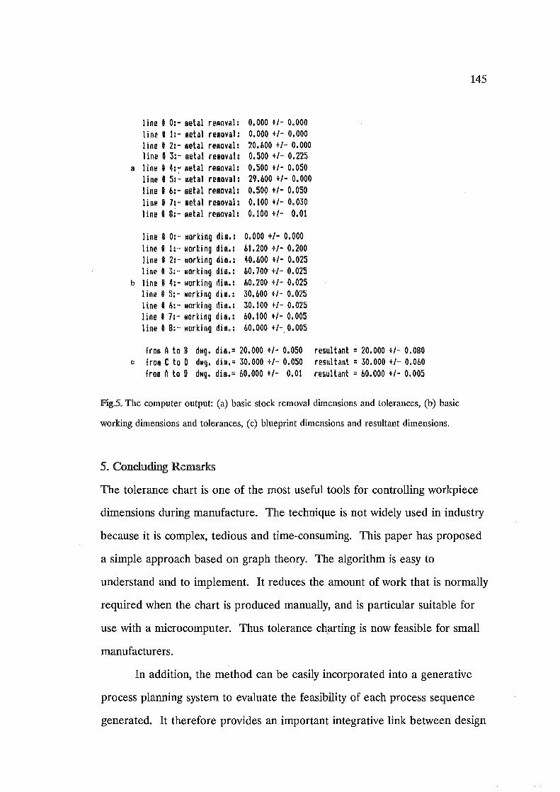
line fi 0:- letal removal: 0.000 +/- 0.000 line. 1:- metal reloval: 0.000 +/- 0.000 line' 2:- letal removal: 20.600 +/- 0.000 line I 3:- letal reloval: 0.500 +/- 0.225

a line' 4:~ metal reloval: 0.500 +/- 0.Q50 line' 5:- letal reloval: 29.600 +/- 0.000 line' 6:- letal reloval: 0.500 +/- 0.050 line. 7:- letal reloval: 0.100 +/- 0.030 line' B:- letal reloval: 0.100 +/- 0.01

line I 0:- ~orking dil.: 0.000 +/- 0.000 line' 1:- Marking diM.: 61.200 +/- 0.200 line' 2:- Marking diu.: 40.600 +/- 0.025 line' 3:- working dim.: 60.70~ +/- 0.025

b line I 4:- working diM.: 60.200 +/- 0.025 line' 5:- Marking dil.: 30.600 +/- 0.025 line I 6:- Marking dil.: 30.100 +/- 0.025 line I 7:- Morking dil.: 60.100 +/- 0.005 line I 8:- ~orking dil.: 60.000 +/-,0.005

frol A to B dNg. dil.= 20.000 +/- 0.050 c frol C to D dwg. dil.: 30.000 +/- 0.050

frol A to D dNg. dim.= 60.000 +/- 0.01

resultant = 20.000 +/- 0.080 resultant = 30.000 +/- 0.060 resultant = 60.000 +/- 0.005

F.xg.5. The computer output: (a) basic stock removal dimensions and tolerances, (b) basic

working dimensions and tolerances, (c) blueprint dimensions and resultant dimensions.

5. Concluding Remarks

145

The tolerance chart is one of the most useful tools for controlling workpiece

dimensions during manufacture. The technique is not widely used in industry

because it is complex, tedious and time-consuming. This paper has proposed

a simple approach based on graph theory. The algorithm is easy to

understand and to implement. It reduces the amount of work that is normally

required when the chart is produced manually, and is particular suitable for

use with a microcomputer. Thus tolerance ch,arting is now feasible for small

manufacturers.

In addition, the method can be easily incorporated into a generative

process planning system to evaluate the feasibility of each process sequence

generated. It therefore provides an important integrative link between design

. and production.

References

1. C. J. Marks, "Tolerance charts control production machining", American Machinist, 97(5), pp. 114-116, March 1953.

146

2. J. F. Anderson Jr., "Assembly tolerance charts save time and money", The Tool Engineer, 37(6), pp. 95-97, December 1956.

3. A. Johnson, "Index tolerance chart simplifies production", The Tool Engineer, 32(2), pp. 53-62, February 1954.

4. C. T. Mooney, "How to adjust tolerance charts", The Tool Engineer, 35(4), pp. 75-81, October 1955.

5. O. R. Wade, Tolerance Control in Design and Manufacturing, Industrial Press, New York, 1967.

6. J. L. Gadzala, Dimensional Control in Precision Manufacturing, McGraw-Hill, New York, 1959.

7. C. F. Sack Jr., "Computer managed process planning a bridge between CAD and CAM", AUTOFACT 4, Philadelphia, Pennsylvania, pp. 7.15-7.31, 30 November - 2 December 1982.

8. R. S. Ahluwalia and A. V. Karolin, "CATC - a computer aided tolerance control system", Journal of Manufacturing Systems, 3(2), pp. 153-160, 1984.

9. T. Xiaoqing and B. J. Davies, "Computer aided dimensional planning", International Journal of Production Research, 26(2), pp. 283-297, 1988.

10. D. F. Robinson and L. R. Foulds, Digraph: Theory and Techniques, Gordon and Breach Science Publishers, New York, 1980.

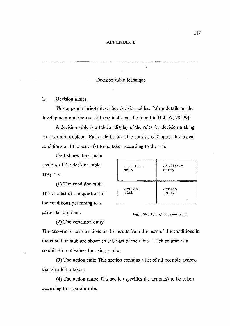
APPENDIX

Decision table technique

1. Deci'iion tables

This appendix briefly describes decision tables. More details on the

development and the use of these tables can be found in Ref.[77t 78t 79].

147

A decision table is a tabular display of the rules for decision making

on a certain problem. Each rule in the table consists of 2 parts: the logical

conditions and the action(s) to be taken according to the rule.

Fig.1 shows the 4 main

sections of the decision table.

They are:

(1) The condition stub:

This is a list of the questions or

the conditions pertaining to a

particular problem.

(2) The condition entry:

condition condition stub entry

action action stub entry

FJg.l: Structure of decision table.

The answers to the questions or the results from the tests of the conditions in

the condition stub are shown in this part of the table. Each column is a

combination of values for using a rule.

(3) The action stub: This section contains a list of all possible actions

that should be taken.

(4) The action entry: This section specifies the action( s) to be taken

according to' a certain rule.

148

Table header Rule header

DECISION TABLE ~ :I 3 4 5

direction of cut face -1 -1 +1 +1 -1

direction of locating face 1 1 +1 +1 +1 +1 -1 -1

position of locating face * relative to cut face c)l Dc c)l l)c c)l

sign of the cut +1 -1 -1 +1 +1 -1

Note: * 1 == locating face, c cut face

Hg.2: Extended-entry table.

Rules

condition 10 [c] 10 [c] 1 n n SIGN = + 0 1 0

action stub action ADD X X

SUBTRACT X

F'Jg3: Limited-entry table.

Fig.2 is called an "extended-entry" table. In this type of decision table,

the elements of the condition entry and condition action have any value.

Fig.3 shows another type of decision table, called a "limited-entryU

table, where the answers to the questions are of YES-NO type. Each element

of the condition entry is either 'Y' for 'yes', 'N' for 'no', or '_' for 'not

149

. applicable'. These values are coded in this figure as follows: '1' for 'Y', '0' for

'N', and 'n' for '_'. AS for the action entry, it consists of 'X' to specify the

action(s) in the action stub to be executed.

CAPPFD uses only limited-entry tables.

2. Processing of decision tables. in CAPPFD

The CAPPFD system uses a subprogram to process the decision tables.

All the condition entry matrices and the lists of conditions to be tested are

passed, by address, from the calling subprograms. If the conditions in the list

match with those in one of the rules, the rule number will be passed back to

the calling subprogram for further action(s). However, if no rule is found, it

will return -1. The flowchart for processing the decision tables is shown in

FigA.

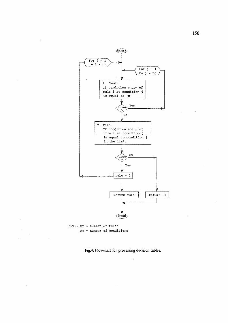
For i ~ 1 to i ~ nr

1. Teet: If condition entry of rule i at condition j is equal to 'n'

Yes

2. Test: If condition entry of rule i at condition j is equal to condition j in the list.

nr number of rules nc = number of conditions

FJg.4: Flowchart for processing decision tables.

150

151

APPENDIXC

Some results from the testing of tolerance chart program

Four sets of the results are presented in this appendix. Each set

consists of two figures, one showing the results from manual calculations, the

other showing the results from the program. The manual calculations are

taken from Ref [61, 63, 67 and 68]. Also shown in the latter are the contents

of the data file for running the program.

152

Set 1:

-.-

~ .-

~ COT lop. FACE ,M/C DIM STOCK DIM. NO. NO COT BASIC +/·TOL. A B IC I E G H I J BASIC I+/-TOL

0 0 1 75.60 0.015 SOl~CI

2 I 19.00 0.005 SOliO 3 60.20 0.030 3 solid 4 ~

o 005 4 0.10 0.025 5 0,010 5 solid 6 14 .80 0010 .6 solid

+R 10 10 0.005 7. solid 21.10 0.005 solid

H'~~ 0005 19 0,10 0.015 i

10 0.003 0 010 0 .. 013 11 0010 ill solid 12 5630 0.003 1 0.10 0.011 13 35.20 0.002 1.3 0.10 0.015 14 11.00 0.003 1. o 10 0.018 15 35.10 0.002 1:' 0 .. 10 0.004

.16 35.00 0,001 1/ 0.10 0.003 17 11.00 0.001 1 0.10 0.007 18 **i 0.001 m '1 010 0.008 19 0.002

~ o 10 0.010

20 18,00 0,002 o 10 0,030 21 3.00 a 004 1 solid

: 22 56,00 0.003 I 0.10 o 004 23 24,00 0.005 2 0.10 0,045

. 24

25 26 27

26 BT. """,,,OU"'LtuHw

29 10 00 ''"'. 10.00 0.005 30 15,00 0.060 15,00 0 .. 055 31 3.00 0,050 3.00 0.004 i

: 32 21.00 0,050 21,00 0.004 33 900 0.060 9.00 0.060 34 15,00 O.O:W I I 15.00 0,011

i 35 17.00 0.010 17,00 0.003

W 4.00 0.020 4.00 0,017

15.00 0.020 15.00 0 .. 020

39 I I , 40 i 41

42 43 44-45

ALL DIMENSIONS ARE IN MILLIMETRES.

FIg.1: Manual calculations of tolerance chart [61].

~ 0:- metal rem~val: fi 1:- metal removal: I 2:- metal removal: * 3:- metal re~oval: # ~:- metal removal: 4 5:- metal removal: I 6:- metal re~oval: i 7:- metal removal: • B:- metal r£!fflt.val: t 9:- metal removal: ~ 10:- metal relllDval: • 11:- metal relDval: II 12:- metal relllt.val: ~ 13:- metal re2Dval: II 14:- metal removal: ~ 15:- metal removal: • 16:- metal rI?!ilt.vill: 4 17:- metal re~Dval: i lll:- ~etal removal: t 19:- !/letal reelClval: 1I 20:- metal removal: * 21:- metal re~Dval: » 22:- metal remDval: * 23:- metal removal:

II 0:-

0.000 +1- 0.000 O.OO(f +1 - 0.000 0.000 +1- 0.0(10 0.000 +1- 0.000 0.100 +l- 0.025 0.000 +1- 0.000 0.00(! f/- 0.0(1(1 0.000 +1- O.OM 0.000 +1- 0.000 0.100 +1- 0.015 0.100 +1- 0.013 0.000 +1- 0.00(1 0.100 +1- 0.011 0.100 +/- 0.015 0.100 +/- O.OIB 0.100 +1- 0.004 (f.l00 +/- 0.003 0.100 +1- (I.M7 0.10(f +1- 0.008 0.100 +1- 0.01\) 0,l{10 +1- (1.030 0.000 +1- 0.000 0.100 +1- 0.004 0.100 +1- (1.045

(I

9 BeE E F G H I J A A D Pi C f 6 H I 10.0 15.0 3.021.0 9.0 15.0 17.0 4.0 15.0 .10 • Ob .05.05 .06. (IE .01 .02.02 23 A J J H H 6 A A A J J H H E E H E H E E E H A J H C A G f B E J H I A E B H E B A J 6 D A F

153

i 1:- Krk. dim.: 75.600 +1- 0.015 I 2:- wrk. dim.: 19.000 +1- 0.005 I 3:- wrk. diM.: 60.200 +/- 0.030 I 4:- wrk. dim.: 56.500 +/- 0.005 ~ 5:- Wit. dim.: 17.300 +/- 0.010 • 6:- _rk. dim.: 14.BOO +/- 0.010 ~ 7:- \'Irk. dim.: 10.100 +/- 0.(105 ~ H: - i!rk. dim.: 21.100 +/- 0.(1(15 I 9:- \'Irk. dim.: 75.4(1(1 +/- 0.005 I JO:- wrk. dim.: 19.(100 +1- 0.003 I 11:- flrk. dim.: 15.100 +1- 0.010

.015 .005 .030 .005 .010 .010 .005 .005 .0(f5 .003 .010 .003 .(102 .(1(13 .002 ,001 .001 .001 .002 .002 .(104 .003 .005 (f 0 (l .1 0 0 (I 0 .1 .1 0 .1 .1 .1 .1 .1 .1 .1 ,1 .1 (I .1 .1 (l 0 0 -1 0 (I (I (I -1 I (I -1 -1 -1 -1 -1 -1 -1 -I I (I -1 -1

~ 12:- wrk. dim.: 56.300 +1- 0.003 ~ 13:- \!Irk. difll.: 35.200 +1- (l.ME ~ 14:- wrk. dim.: 11.000 +1- 0.003 1I 15: - "rko dim.: 35.10{l +1- 0.002

(a) Contents of data me.

1I 16:- wrk. dim.: 35.(1(10 +/- 0.001 • 17:- lIrko di~.: 11.000 +1- O.OO! 1I 18:- wrk. dim.: 56.100 +1- 0.001 I 19:- wrko dim.: 54.000 +1- 0.002 t 20:- wrY.. dim.: 18,000 +1- 0,002 t 21:- IIrL dlle.: 3,000 'r/- 0.004 # 22:- ~lrk. dim.: 56.000 +/- 0.003 I 23:- lIit. dim.: 24.000 +/- 0.005

froll B to A: dWf]. dim.'" 10.000 +1- 0.100; resultant", 10.000 +J- 0.005 fft<m C b Pi: dlif]. dill.: 15.000 t/- 0.060; resultant;:; 15.000 +/- 0.055 frolJl E tel D: dwg. dim.'" 3.00(1 +/- 0.050, resulhnt = 3.000 +1- 0.004 frCtfil E to I'll dwg. dim.;:; 21.000 +1- 0.050; resultant;:; 21.000 +1- (1,004 from F ttl C: dwg. dim.: 9.000 +1- 0.060; resultant;:; 9,(1(10 t/- 0.060 frer& 6 to F: dllf]. dim.: 15.OQO +1- 0.02(f~ Ti!Sultimt ;:; 15.000 +1- 0.011 fro/) H tel Ih dwg. dlalo= 17.000 +/- 0.010; resultant;:; 17.000 +1- 0.003 frt.1ll I it. H:- dllg. dim." 4.0(1(1 +1- 0.020; resultant" 4.000 +1- 0.017 from J ttl I: d~jg. dim.= 15.(1()0 +1- (1.020; resultant;:; 15.000 +1- 0.020

F.ag.2: Data me and computer outputs.

(b) Computer outputs.

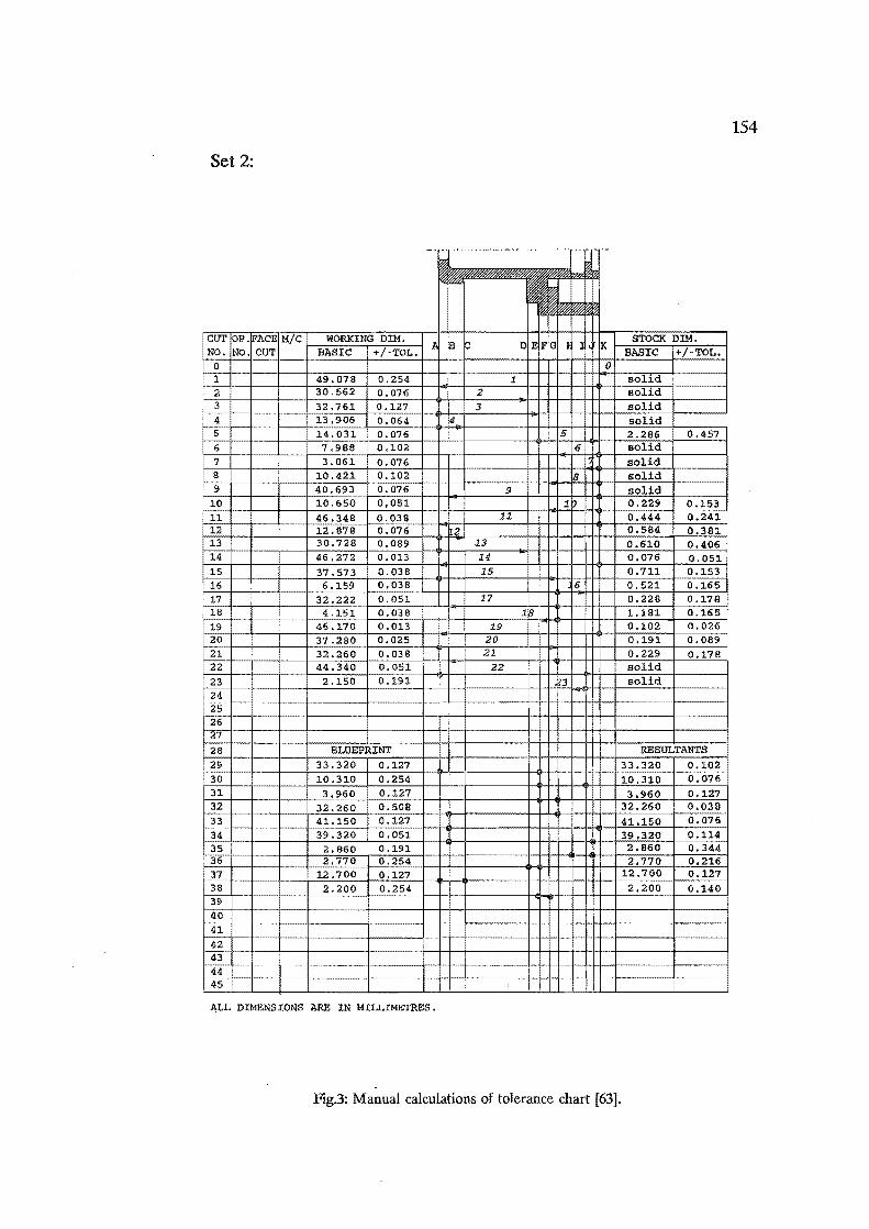
154

Set 2:

_. -.-.-.-.-.-.~.---~

CUT OP fACE M/c DIM, STOCK DIM }, Is c D K

,NO. NO, I CUT BASIC +/'TOL, BASIC I+/-TOL 0 _0 1 49,078 0.254 1 solid 2 30.562 0,076 2 solid 3 32.761 0,127 3 solid 4 13 .906 0,064 14 solid S"" 14,031 0,076 5 2.286 0.457 6 7,988 0,102 6 solid 7 3,061 0,076 solid 8 10,421 0,102 8 solid 9 40,693 0,076 9

~ solid

10 10650 0,051 0,229 0.153 11 46,348 0,038 11 0.444 0.241 12 12,878 0.076 n2 0.584 0,381 13 30.728 0.089 • 13 0.610 0,406 14 46,272 a 013 14 0.076 0.051 15 37,573 0,038 15 0,711 0153 16 I 6 159 0,038 6111 0.521 OHi5 17 32,222 0,051 17 0.228 0.178 18 4 151 0.038 ..!:.~ 1.181 0,165

, 19 I 46,170 0,013 0.102 0.026 20 37.280 o 025 0191 0,089 21 32.260 0.038 21 0.229 0.178 22 44.340 0.051 22 solid 23 2 150 0.191

Iff solid

i 24 I 25

26 27

28 l>T .. l)l7.l'!TlT .'T'll "lT~

29 33.320 0.127 33,320 0,102 30 10.310 0.254 10310 0,076 31 3'960~ 3,960 0.127 32 32,260 32 260 0.038 33 41.150 41,150 0.076 34 39.320 0.051 39,320 0.114 35 2,860 0.191 2.860 a 344 36 :2 770 0.254 2.7 o 216 37 12,700 a 127 12.700 ° 127 38 2,200 0,254 2200 0.140 39 40 41 42 43 44 45 . ALL DIMENSIONS ARE IN MILLIMETRES.

Fig3: Manual calculations of tolerance chart [63].

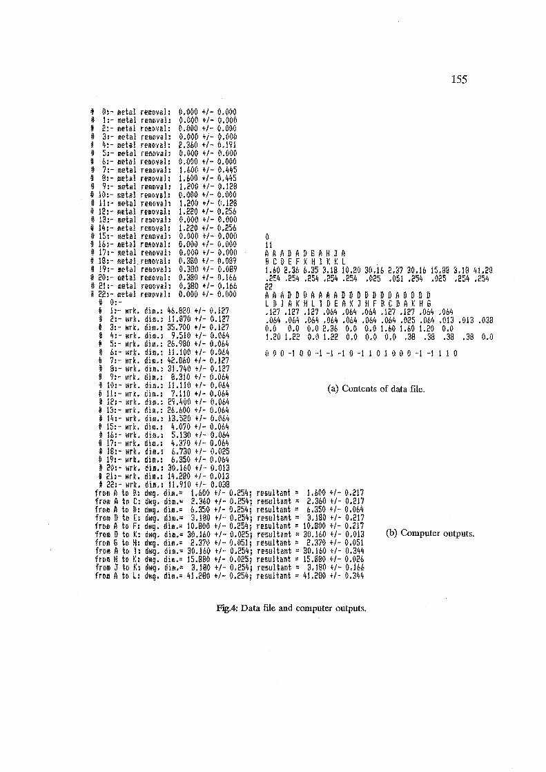
# 0:- metal removal: # 1:- metal removal: • 2:- metal refioval: » 3:- metal removal: I 4:- metal removal: D 5:- metal re~~val: • b:- metal removal: I 7:- metal removal: ~ B:- metal removal: # 9:- metal removal: # 10:- letal remctvah » 11:- metal reroctvah i 12:- metal reloval: I 13:- metal removal: I 14:- metal removal: » 15:- metal removal: t Ib:- metal removal: D 17:- metal removal: ~ IB:- ~etal.removal:

(}

11 A A A DAD S A H J A BCD E F K H I K K L .

155

I 19:- metal removal: I 20:- metal removal: I 211- metal removal: fl 22:- metal removal:

0.000 +/- 0.000 0.000 +/- O.OM 0.000 t/- 0.000 0.000 +/- 0.000 2.360 t/- 0.191 0.000 +/- 0.000 0.000 t/- 0.000 1.600 +/- 0.445 l.bOO +1- 0.445 1.200 t/- 0.12B 0.000 t/- 0.000 1.200 +/- 0.12B 1.220 +J- 0.256 0.000 +1- 0.000 1.220 +/- 0.256 0.000 +/- 0.000 {!.OOO +1- 0.0(10 0.000 +/- 0.000 0.330 +/- 0.089 (1.3BO +/ - (1.089 0.3BO +/ - (1.166 0.380 +1- 0.166 0.000 +/- 0.000

1.60 2.36 6.35 :LIB 10.8Q 30.16 2.37 30.16 15.118 3.13 41.28 .254 .254 .254 .254 .254 .025 .051 .254 .025 .254 .254 22

» 0:-A A ADD D A A A ADD D D D D DAD 0 D D l D I A K H lID E A K J H F BCD A K H G

i h- Nrk. dim.: 46.B20 +/- 0.127 i 2:- wrk. dim.: 11.870 +/- 0.127 I 3:- Nrk. dim.: 35.700 +/- 0.127 I 4:- wrk. dim.: 9.510 +/- 0.Ob4 t 5:- "rk. dim.: 2b.980 +/- 0.064 * 6:- wrk. dim.: 11.100 +/- 0.064 4 7:- "rk. dim.: 42.860 +/- 0.127 I H:- wrk. dim.: 31.740 +/- 0.127

.127 .127 .127 .Q64 .064 ,064 .127 .127 .064 .064 .(164 .064 .004 .OM .%4 .OM .Ob4 .025 .064 .013 .!H3 .038 0.0 0.0 0.0 2.36 0.0 0.0 l.bO 1.60 1.20 0.0 1.20 1.22 0.0 1.22 0,(1 0.0 0.0 .38 .3B .38 .38 0.0

(I (; 0 -I 0 (I -1 -1 -1 0 -1 1 0 1 0 (I 0 -1 -I ! 1 0

j 9:- wrk. dim.: B.310 +1- 0.064 I 1(1:- wrk. dim.: 11.110 +/- 0.064 i 11:- "rk. dim.: 7.110 +/- 0.064 I 12:- wrk. dim.: 29.400 t/- O.OM

(a) Contents of data file.

# 13:- wrk. dif..: 26.600 t/- 0.064 i 14:- wrk. dim.: 13.520 t/- 0.064 t 15:- wrk. di~.: 4.070 t/- 0.064 # 16:- wr!:. dim.~ 5.130 t/- (1.064 t 17:- "TI:. dilll.~ 4.370 +/- O.OM I 18:- wr~. dim.: 6.730 t/- 0.025 1I 19: - wrL dim.: 6.350 +J- 0.064 .. 20:- wrk. dim.: 30.160 t/- 0.013 i 21~- wrt. dim.: 14.280 t/- 0.013 .. 22;- wrL dim.: 11.910 +1- 0.03B

from A ttl B: dwg. dilll." 1.(,Jj(l +J- 0.254; resultant" 1.600 +J- 0.217 frr.Jl A tr< C: dwg. dim." 2.360 t/- 0.254; resultant" 2.3bO +/- 0.217 fre'A! A tc< D: dltg. dim.= 6.350 tJ- 0.254; resultant:: 6.350 +1- 0.064 from D tn E: dwg. dim.= 3.1BO t/- 0.254; resultant" 3.180 t/- 0.217 from A toF: dwg. di~.= 10.800 +/- 0.254; resultant := 10.BOO +1- 0.217 from D to K: dwg. die." 30.160 t/- 0.025; resultant" 30.160 +/- 0.013 fro~ G to H: dwg. dim.: 2.370 +/- 0.051; resultant: 2.370 +/- 0.051 frolS A tCt I: dwg. dia.: 30.160 t/- 0.254; resultant: 30.160 t/- 0.344 fro~ H to Vol dwg. dil.: 15.9BO +/- 0.025; resultant: 15.BBO +/- 0.026 from J to ¥o: dwg. dim.= 3.180 t/- 0.254; resultant" 3.190 +/- 0.166 from A ic, l: dlilg. dim.= 41.280 t/- 0.254; resultant := 41.290 +1- 0.344

FJg.4: Data file and computer outputs.

(b) Computer outputs.

156

Set 3:

ALL DIMENSIONS ARE IN MILLIMETRES.

F'tg.5: Manual calculations of tolerance chart [67].

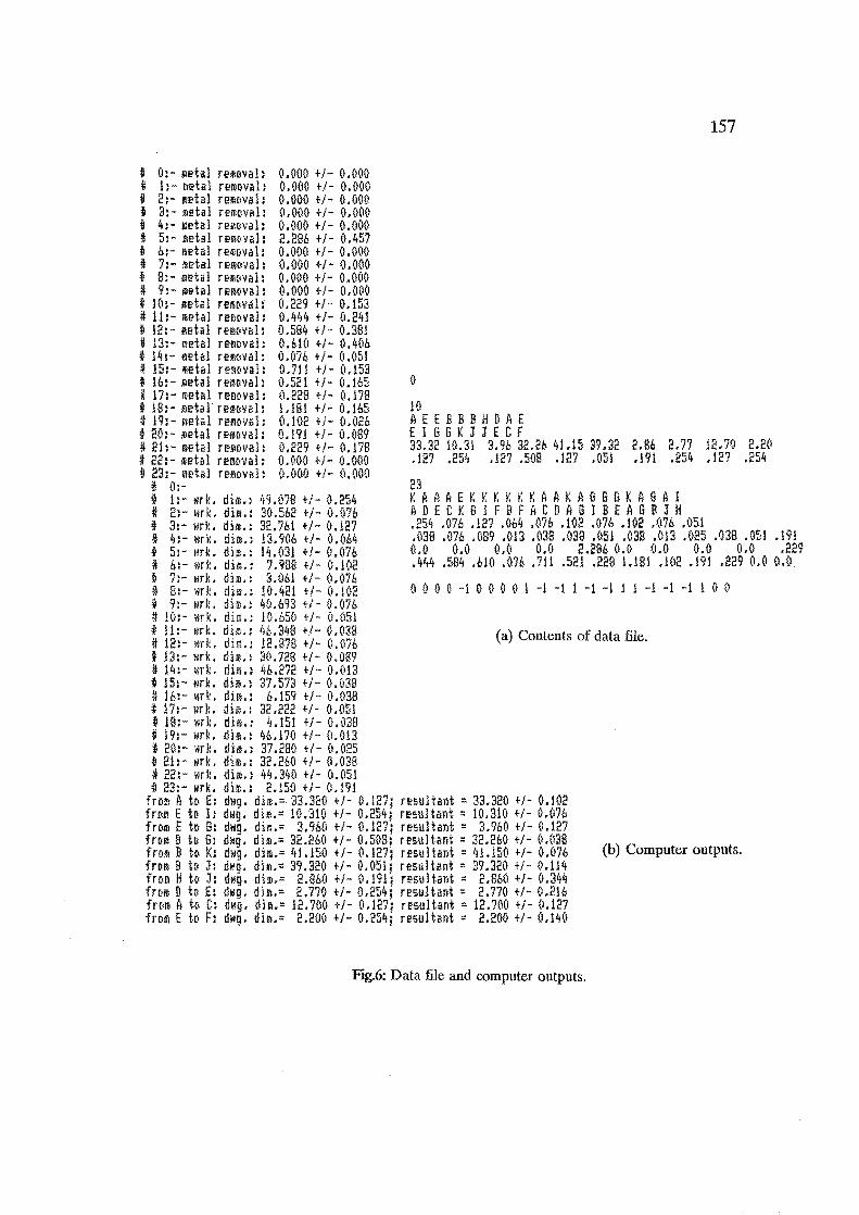
I 0:- ~etal removal: 0.000 +/- 0.000 * 1:- l'Ietal removal: 0.000 +./- 0.(100 4 2:- rletal remDval: 0.000 +/- 0.000 II 3:- lIletal removal: {l.OM +/- 0.000 I 4:- metal re~Dval: 0.000 +/- 0.000 # 5:- .!Iehl remc"Jal: 2.296 +/- 0.457 II 6:- metal remDval: 0.000 +/- 0.000 # 7:- ~etal removal: 0.000 +/- 0.000 II B:- metal remc.nl: 0.000 +/- 0.000 fi 9:- metal removal: 0.000 +/- 0.(1(10 I 10:- letal felllovll: ·0.229 +/- 0.153 I 11:- ~etal removal: 0.444 +/- 0.241 ti 12:- "etal re~oval: 0.584 +/- 0.381 I 13:- metal remBval: 0.610 +/- 0.406 t 14:- metal remDval: 0.076 +/- 0.051

o 10 A E EBB B H D A E E I G G V. J J E C F

157

1I 15:- metal removal: 0.711 +/- 0.153 ~ 16:- metal removel: 0.521 +/- 0.165 I 17:- metal removal: 0.228 +/- 0.17B e Hl:- l'letalremDval: 1.1£11 +/- 0.165 II 19:- Riet.al removal: 0.102 +/- 0.02& I 20:- letal remDval: 0.191 +/- 0.089 II 21:- metal removal: 0.229 +/- O.I/B ~ 22:- metal ru(.vill: 0.000 +/- 0.000 ~ 23:- llIeta! remo'!i'!!: (l,O(W +J- 0.000

33.32 10.31 3.96 32.2b ql.15 39.32 .127 .254 .127 .508 .127 .051

2.B6 2.77 12.70 2.20 .191 .254 .127 .254

23 II 0:-II 1:- wrk. dim.: 4'1.07B +/- 0.2'54 # 2:- wrk. dim.: 30.562 +/- 0.076 # 3:- wrY., dim.: 32.761 +/- 0.127 # 4:- wrY.. dim.: 13.906 +/- 0.064 I 5:- wrk. di~.: 14.031 +/- 0.076 ~ 6:- wrL dim.: 7.99B +1- 0.102 I 7:- wrk. dim.: 3.061 +/- 0.076 jj B:- I'lrk. dim.: 10.421 +/- 0.102 j 9:- wrk. dim.: 40.693 +/- 0.076 ,J! 10:- wrk. dim.: 10.bSO +J- 0.051

K A A A E KKK K ~ K A A K A 8 G 6 K A 6 A I A DEC Y. G I F BFA C D A G I B E A G B 1 H .254 .on .127 .004 .076 .102 .076 .102 .{I76 .OSI .03B .076 .099 .013 .038 .038 .051 .038 .013 .025 .Q38 .051 .191 0.0 0.0 0.0 0.0 2.2B6 0.0 0.0 0.0 0.0 .229 .444 .584 .610 .076 .711 .521 .229 UBI .W2 .191 .229 0.0 0.0

o (I 0 0 -1 0 0 0 (I 1 -1 -1 1 -1 -1 1 1 -1 -1 -I I 0 0

1I 11:- wr!:. dim.: i,id4!l t/- 0.03B # 12:- wrY.. dim.: 12.378 +/- o.on t 13:- \irk. dim.: SO.nll +/- 0.089

(a) Contents of data me.

i 14:- ~lrL dim.: 46.272 +/- (1,013 t 15:- wrk. di~.: 37.573 +/- 0.03B I 16:- .rk. dim.: b.IS9 +/- 0.038 i 17:- wrl:. dil/i,: 32.222 +/- 0.051 • 18:- wrk. dia.: 4.151 +/- 0.039 I 19:- Nr~. dim.: 46.170 +J- 0.013 ¥, 20:- wrk. dim.: 3/.230 +/- 0.025 I 21:- l>IrL dim.: 32.2HI +/- 0.038 I 22:- wrk. di •• : 44.340 +/- 0.051 jj 23:- wrk. dim.: 2.150 +/- 0.191

from A to E: dWQ. dim.:· 33.320 +/- 0.127; resultant = 33.320 +J- 0.102 frofi E to I: dwi. dim.= 10.310 +/- 0.254; resultant = 10.310 +/- 0.076 frc.m E trr Il: dHQ. dim.= 3.9bO +/- 0.127; resultilnt:: 3.960 +/- 0.127 from II til G: dilg. dim.= 32.260 +/- 0.503; rl?Sultilnt :: 32.260 +/- 0.038 frc,P.i Ii t« K: dwg. dim.:: 41.150 +/- 0.127; resultant = 41.150 +/- 0.076 fnm B t(. J: dwg. dirl,::: 39.320 +1- 0.051; resultant = 39.320 +/- 0.114 frolll H tel J: difg. dim,: 2.B6O +/- 0.191; resultant::: 2.abO +/- 0.344 from D t« EI dllg. dim.'" 2.710 +/- 0.254; rl?sultant = 2.770 +/- 0.216 frr'ffJ fI tel C: dwg. dilli.= 12.700 +/- 0.127, resultant = 12.700 +/- 0.127 frOID E to F: df/g. dill'l.::: 2.2(10 +/- 0.254; resulhnt = 2.200 +/- 0.140

FJg.6: Data me and computer outputs.

(b) Computer outputs.

158

Set 4:

WORKING DIM. STOCK DIM. BASIC +/-TOL. BASIC +/-TOL.

1.594 0.031 0.750 0.031

1.750 0.031 0.750 0.031 4.094 0.062 2.437 0.005 1. 594 0.005 0.072 3.937 0.005 8 0.094 0.041 0.625 0.015 9 solid 0.809 0.010 solid 1.588 0.003 0.088 0.013 2.162 0.003 a 088 0.044 3.338 0.088 0.044

0.031 0.025

0.025 0.008 solid

17 0.625 1 18 3.937 19 1.875 20 3.625 21 0.125 22 5.250 23 0.732 0.030 24 3.786 0.010 0.040 • 25 0.750 0.005 0.018 0.015 26 3.750 0.001 0.018 0.026

.27 0.719 0.002 0.006 0.020 2.469 0.006 0.020

0.006 0.020 0.006 0.020

RESULTANTS 0.125 0.010

0.015 34-

• 35 .36

37 38 39 0.719 40 1.281 0.002 41 2.469 0.002 2.469 42 3.031 0.002 3.031 43 3.750 0.001 3.750

5.250 0.002 5.250 5.500 0.015 5.500

ALL DIMENSIONS ARE IN INCHES.

Fig.7: Manual calculations of tolerance chart [68].

t 0:- metal rell[tval: li h - metal relllt<val: t 2:- Dehl rellc.vai: $ 3:- metal rem~val: * 4:- Jletal refllclval: 1\ 5:- lIIetal re!llc''1al: I b:- Jletal reloval: i 7:- metal remDval: t B:- metal r~m~val: ~ 9:- metal removal: .jj 10: - fietal remelvab .jj 11:- metal removal: 4 12:- metal removal: i 13:- metal remc.val: t 14:- lIletal removal: I 15:- metal removal: , 16:- lIletal remDval: t 17:- metal TeJloval: I 18:- lIletal re~Dvall # 19:- metal removal: II 20:- metal re.ll1oval: li 21:- met~l removal: I 22:- letal removal: i 23: - metal relllc.val: I 24:- metal refiDval: i 25:- metal removal: i 2b:- !'letal reIllD'Ial: * 27:- metal removal: t 28:- metal remDval: .jj 29:- metal removal: i 30:- metal removal:

.jj 0:-

0.0(1(1 +/- 0.000 0.000 +/- 0.000 0.0(\(\ +/- 0.00(1 0.00(1 +/- 0.000 0.000 +/- 0.000 0.000 +/- 0.000 0.063 +i- 0.Ob7 0.Ob3 +/- 0.072 0.094 +/- 0.041 0.000 +/- 0.000 0.000 + /- 0.000 (I.osa +/- 0.013 0.09B +/- 0.044 0.OB8 +/- 0.044 0.031 +/- 0.025 0.025 +/- 0.008 0.000 +/- O.IJOO 0.(1(10 +/- 0.000 0.0(1(1 +/- 0.000 0.(100 +/- 0.000 0.000 +/- 0.000 0.000 +/- 0.000 0.000 +/- 0.000 0.048 +/- 0.030 O.MB +/- 0.040 0.018 +/- (1,015 0.018 +/- 0.026 0.006 +/- 0.020 O.(lOb +/- 0.020 O.OOb +/- (1.020 O.OOb +J- 0.020

5 A F F I F F H 1 K 0 0.031 0.031 0.031 0.031 0.Ob2 14 A A A " A A E D D D D DBA BCD 0 6 J 0 F H I K L N 0

159

t 1:- stt:. dim.: 1.5'14 +/- 0.031 (A-F) j) 2:- stc. dim.: (1.750 +J- 0.031 iF-H) t 3:- stc. dim.: 1.751J +/- O.Cl31 IF-I} I 4:- stc. dim.: 0.750 +/- 0.031 II-Kl j 5:- stc. dim.~ 4.094 +/- 0.062 IF-D) II b:- wrk. dil.: 2.437 +/- 0.005

.125 .b25 .875 .b25 1.875 3.625 3.937 .719 1.281 2.469 3.031 3.750 5.250 5.500 .015 .015 .015 .Ot5 .015 .015 .0!5 ,002 ,002 .002 .002 .OO} .002 .015 25

i 7:- wrk. dim.: 1.594 +/- 0.005 jJ 8:- wrL dim.: 3.937 +/- 0.005 t 9:- lirl:. dim.: 0.625 +/- 0.015 I 10:- wrk. di~.: 0.809 +/- 0.010 i 11: - wrk. dim.: 1.5B8 +/- 0.003

F K K A A A A A A A ADD A A A B B D B D D D D D K 0 A C D F HID K L M E 6 J B N D L D L F 1 H K ,~05 .005 .005 .015 .010 .003 ,003 .003 .015 .003 .tHO .015 .015 .015 .015 .010 .002 .OHI .010 ,005 .001 .002 .002 .002 .0(12

• 12:- wrk. dim.: 2.162 +i- 0.003 i 13:- wrk. dim.: 3.338 +/- 0.003 I 14:- wrk. dim.: 5.500 +/- 0.015

.063 .063 .094.0 .0 .088 .{ISS .08B .031 .025

.0 .0 .0 .0 .0 .0 .0 .048 .048 .018

.018 .00b .00b .00b .006 t 15:- wrk, di0.: 3.912 +/- 0.003 -1 -I -1 0 (I 1 -1 1 -I -1 0 0 0 0 (I 0 0 1 -1 1 -1 1 1 -1 -I D 16:- wrk. dim.: 4.b91 +/- 0.010 I 17:- "rk. dim.: 0.625 +/- 0.015 I 18:- wrk. dim.: 3.937 +/- 0.015 * 19:- wrk. dim.: 1.875 +/- 0.015 I 20:- !irk. dim.: 3.625 +J- 0.015 I 21:- wrk. dim.: 0.125 +/- 0.010 II l!2:- wr!:' dim.: 5.250 +/- 0.002 I 23~- !irk. dim.: 0.732 +/- 0.010 I 24:- Mrk. dift.: 3.786 +/- 0.010 i 25:- wrY.. dim.: 0.750 +/- 0.005 I 2b:- \<Irk. dim.: 3.750 +/- 0.001 i 27:- "rk. dim.: 0.719 +/- O.OOE ~ 28:- wrk. dim.: 2.469 +/- 0.002 j 29:- wrk. dim.: 1.281 +/- 0.002 I 30:- "rk. dim.: 3.031 +/- 0.002

from A to B: dwa. dim.: 0.IE5 +/- 0.015; resultant :: frol A tCI C: dVlg. dim.= 0.b25 +/- 0,015; resultant: froll A to D: dflg. dim.= 0.975 +/- 0.015; resultant :: fre.m K to 0: dwg. diM.: 0.625 +/- 0.015; resultant :: from A to G: dwg. dim.: 1.875 +/- 0.015; resultant :: fr~m A to J: dwg. dim.:: 3.625 +/- 0.015; resultant: frc,~ E te. 0: dwg. dim.= 3.937 +/- 0.015; resultant :: frolll D tel F: dwg. dim.= 0.719 +/- 0.002; rl?5ultilllt :: from D tD H: dwg. dim.:: 1.281 +/- 0.002j resultant = frclri D te. 1: dwg. dim.= 2.469 +/- 0.002; resultant = ffl.llll D h ~:: dwg. dill.:: 3.031 +/- 0.002; resultant :: from D to L: dwg. dim.= 3.750 +/- 0.001; resultant = fr()/ll B tc Ii: dwg. dim.:: 5.250 +/- 0.002; resultant :: from A ttl 0: dwg. dim.::: 5.500 +/- 0.015·; resultant ::

(a) Contents of data file.

0.125 +/- 0.010 0.b25 +/- 0.015 0.875 +/- 0.015 0.b25 +/- 0.015 1.875 +/- 0.015 3.625 +/- 0.015 3.937 +/- 0.015 0.719 +/- 0.002 1.281 +/- 0.002 2.469 +/- 0.002 a.031 +/- 0.002 3.750 +/- O.M} 5.250 +/- 0.002 5.500 +/- 0.015

(b) Computer outputs.

FIg.8: Data file and computer outputs.

160

APPENDIXD

The method of traces for checking accumulated tolerance

The following is the excerpt on the method of traces taken from Ref

[61]. Prior to the rooted-tree method, it was commonly used in manual

tolerance charting. The method is presented here for a comparison with the

method developed in this project.

To Check the Accumulation of the Balance-dimension Tolerances and

the Resultant-dimension Tolerances:

1. Trace upward simultaneously from the left and the right

extremity of the dimension in question.

2. Make a horizontal turn with the trace which first encounters an

arrowhead of a working dimension.

3. With that trace move horizontally to the end of that working

dimension, and then turn vertically upward.

4. With the other trace move in a similar fashion along its path.

5. As necessary for convergence (see step 6) continue with both

traces to the next arrowheads and repeat step 3 for each.

6. At the point where both traces converge, the process stops.

(Convergence of traces is defined as the first point at which

both traces would be going upward along the same vertical line.

Remember that the crossing of traces is not convergence!)

7. Add all the tolerances of the working dimensions where

161

horizontal turns were made. This total is the tolerance for the

balance or the resultant dimension in question.

NOTE: Stock-dimension tolerances are not and must not be used at

any time in the foregoing steps.

To Check the Accumulation of Stock-removal Tolerances for Each

Working Dimension:

The same procedure is followed as for the balance and resultant

dimensions (shown above), except that the tolerance of the working

dimension for which the stock-removal tolerance is required must also be

added to the total. Those will result in the stock-removal tolerance at this

working dimension.

Examples

Let us examine several representative examples which show how this

method works.

OPER. WORK DIM. TOL. BAL.DIM.TOL.

10 :to.010 CD·········

:to .• 010 ~ ..... ~. ..,

"f-T--r-~'O:'::'="JI

FIg.l: Calculation of balance-dimension tolerance.

162

Example 1 (Fig. 1 )

The traces (broken lines) are shown beginning at the left and the right

extremities of the balance dimension in question. The point of convergence is

circled. Two horizontal turns are made. These are valued at + 0.010 each, or a

total of + 0.020, which is the tolerance for the balance dimension. Note that

the mean dimensions are not necessary for this check. Also in the actual

practice the paths of the traces are not shown on the tolerance chart. They

are used here to illustrate the method.

Example 2 (Fig.2)

In this example a resultant dimension is computed in a manner similar

to Example 1 for a balancewdimension tolerance. Notice how the traces cross

each other and where convergence takes place.

... -- ----I--- ,- --

Ol?ER. WORK DIM.TOL. BAL.DIM.TOL.

10 ±0.010 I , ,

+0.010 y:~- "'" -----" '-=V .:

20 +0.003 . . ........... -'.,' ... _'--; :

. . . . 30 +0.003

! •••• __ ••••

• !-<iI, ----r,----. : !

RESULTANT DIM.TOL.

FJg2: Calculation of resultant-dimension tolerance.

Example 3 (Fig.3)

In this example the method of traces is used to check a stock-removal

163

. tolerance. The method is the same as for balance- and resultant-dimension

tolerances except that the tolerance of the working dimension for which the

stock-removal tolerance is computed is also added to the total.

.- -'-'---'-'- _._._._._._.

OPER. WORK DIM. TOL.

10 xO.Ol0

to.01O

±0.003

.. r:N' ;-:v

STOCK REM. TOL •

+0.0131

Fig.3: Calculation of stock-removal tolerance.