+ Comparing Two Means Introduction In the previous section, we developed methods for comparing two...

+Co

mp

arin

g T

wo

Mea

ns

Introduction

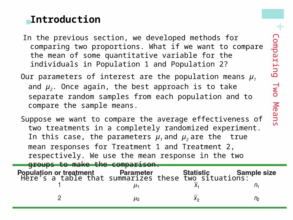
In the previous section, we developed methods for comparing two proportions. What if we want to compare the mean of some quantitative variable for the individuals in Population 1 and Population 2?

Our parameters of interest are the population means µ1 and µ2. Once again, the best approach is to take separate random samples from each population and to compare the sample means.

Suppose we want to compare the average effectiveness of two treatments in a completely randomized experiment. In this case, the parameters µ1 and µ2 are the true mean responses for Treatment 1 and Treatment 2, respectively. We use the mean response in the two groups to make the comparison.

Here’s a table that summarizes these two situations:

+ Section 13.1Comparing Two Means

After this section, you should be able to…

DESCRIBE the characteristics of the sampling distribution of the difference between two sample means

CALCULATE probabilities using the sampling distribution of the difference between two sample means

DETERMINE whether the conditions for performing inference are met

USE two-sample t procedures to compare two means based on summary statistics or raw data

INTERPRET computer output for two-sample t procedures

PERFORM a significance test to compare two means

INTERPRET the results of inference procedures

Learning Objectives

+

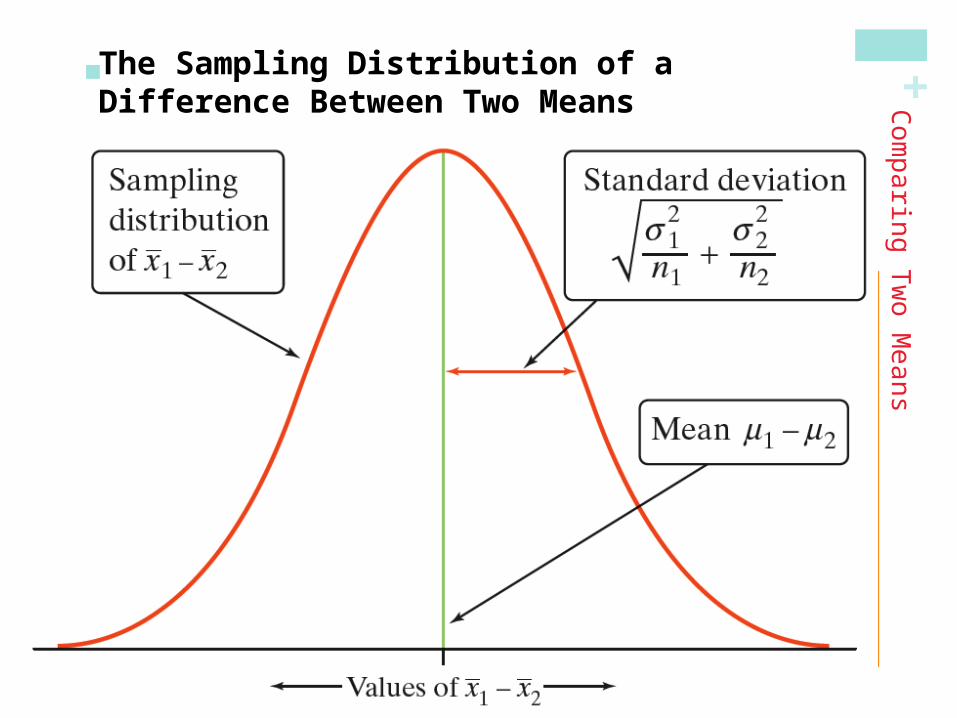
The Sampling Distribution of a Difference Between Two Means

In Chapter 7, we saw that the sampling distribution of a sample mean has the following properties:

Co

mp

arin

g T

wo

Mea

ns

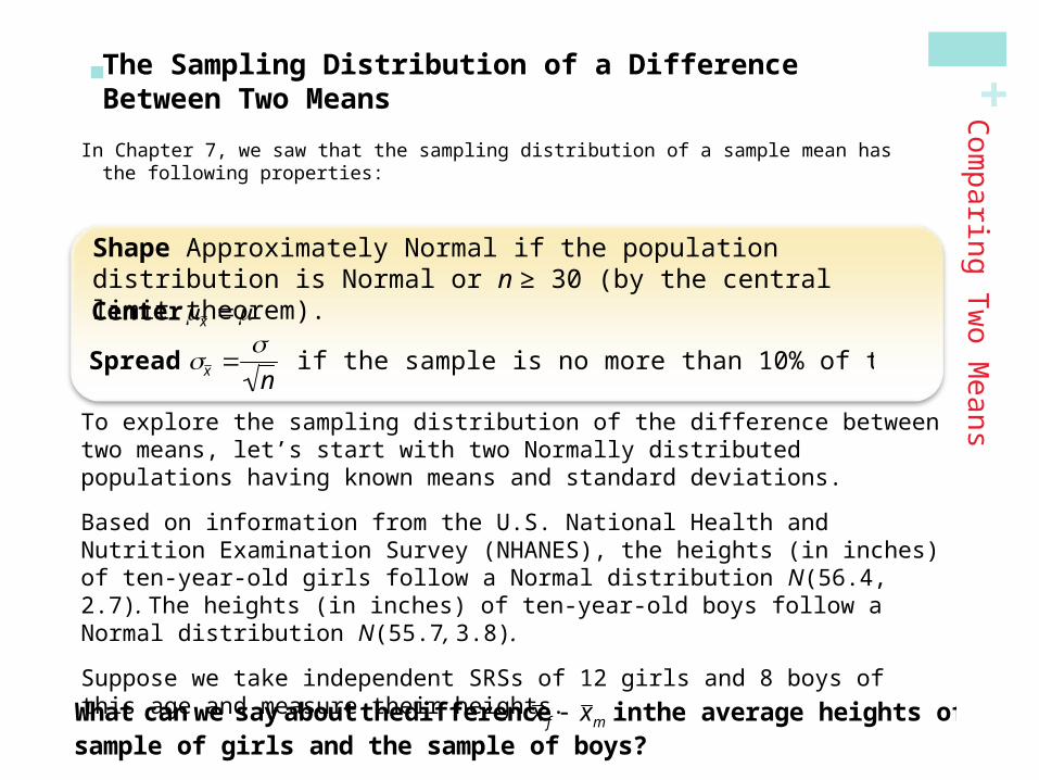
To explore the sampling distribution of the difference between two means, let’s start with two Normally distributed populations having known means and standard deviations.

Based on information from the U.S. National Health and Nutrition Examination Survey (NHANES), the heights (in inches) of ten-year-old girls follow a Normal distribution N(56.4, 2.7). The heights (in inches) of ten-year-old boys follow a Normal distribution N(55.7, 3.8).

Suppose we take independent SRSs of 12 girls and 8 boys of this age and measure their heights.

What can we say about the difference x f x m in the average heights of thesample of girls and the sample of boys?

Shape Approximately Normal if the population distribution is Normal or n ≥ 30 (by the central limit theorem).

Center x

Spread x n

if the sample is no more than 10% of the population

+ The Sampling Distribution of a Difference Between Two Means

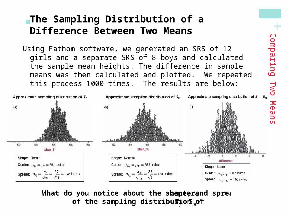
Using Fathom software, we generated an SRS of 12 girls and a separate SRS of 8 boys and calculated the sample mean heights. The difference in sample means was then calculated and plotted. We repeated this process 1000 times. The results are below:

Co

mp

arin

g T

wo

Mea

ns

What do you notice about the shape, center, and spreadof the sampling distribution of x f x m ?

+ The Sampling Distribution of a Difference Between Two Means C

om

pa

ring

Tw

o M

ean

s

Both x 1 and x 2 are random variables. The statistic x 1 - x 2 is the differenceof these two random variables. In Chapter 6, we learned that for any two independent random variables X and Y, X Y X Y and X Y

2 X2 Y

2

Therefore,x 1 x 2

x 1 x 2

1 2

x 1 x 2

2 x 1

2 x 2

2

1

n1

2

2

n2

2

1

2

n1

1

2

n2

x 1 x 2

12

n1

1

2

n2

Choose an SRS of size n1 from Population 1 with mean µ1 and standard deviation σ1 and an independent SRS of size n2 from Population 2 with mean µ2 and standard deviation σ2.

The Sampling Distribution of the Difference Between Sample Means

Center The mean of the sampling distribution is 1 2. That is, the difference in sample means is an unbiased estimator of the difference in population means.

Shape When the population distributions are Normal, the sampling distribution of x 1 x 2 is approximately Normal. In other cases, the sampling distribution will be approximately Normal if the sample sizes are large enough ( n1 30,n2 30).

Spread The standard deviation of the sampling distribution of x 1 x 2 is

1

2

n1

2

2

n2

as long as each sample is no more than 10% of its population (10% condition).

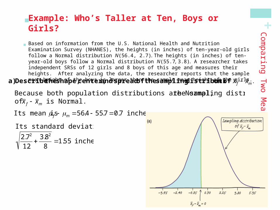
+ Example: Who’s Taller at Ten, Boys or Girls? Based on information from the U.S. National Health and Nutrition Examination Survey

(NHANES), the heights (in inches) of ten-year-old girls follow a Normal distribution N(56.4, 2.7). The heights (in inches) of ten-year-old boys follow a Normal distribution N(55.7, 3.8). A researcher takes independent SRSs of 12 girls and 8 boys of this age and measures their heights. After analyzing the data, the researcher reports that the sample mean height of the boys is larger than the sample mean height of the girls.

Co

mp

arin

g T

wo

Mea

ns

. mf xx of ondistributi sampling the of spread and center, shape, the Describe a)

Because both population distributions are Normal, the sampling distribution of x f x m is Normal.

Its mean is f m 56.4 55.7 0.7 inches.

Its standard deviation is

2.72

12 3.82

81.55 inches.

+ Example: Who’s Taller at Ten, Boys or Girls?C

om

pa

ring

Tw

o M

ean

s

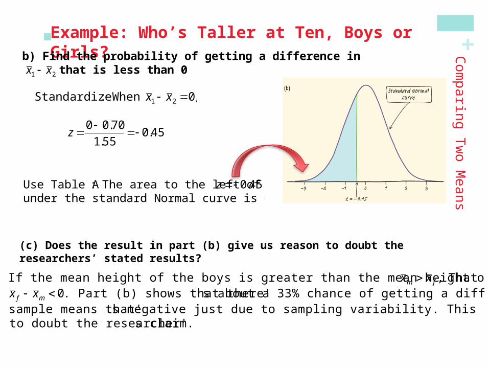
b) Find the probability of getting a difference in sample means x 1 x 2 that is less than 0.

Standardize: When x 1 x 2 0,

z 0 0.70

1.55 0.45

If the mean height of the boys is greater than the mean height of the girls, x m x f , That is x f x m 0. Part (b) shows that there's about a 33% chance of getting a difference in sample means that's negative just due to sampling variability. This gives us little reason to doubt the researcher's claim.

Use Table A : The area to the left of z 0.45 under the standard Normal curve is 0.3264.

(c) Does the result in part (b) give us reason to doubt the researchers’ stated results?

+ The Two-Sample t StatisticC

om

pa

ring

Tw

o M

ean

s

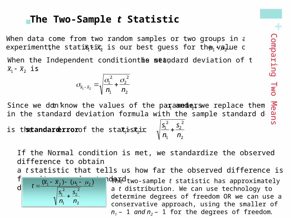
When data come from two random samples or two groups in a randomized experiment, the statistic x 1 x 2 is our best guess for the value of 1 2 .

When the Independent condition is met, the standard deviation of the statistic x 1 x 2 is :

x 1 x 2

12

n1

2

2

n2

Since we don't know the values of the parameters 1 and 2, we replace them in the standard deviation formula with the sample standard deviations. The result

is the standard error of the statistic x 1 x 2 : s1

2

n1

s2

2

n2

If the Normal condition is met, we standardize the observed difference to obtaina t statistic that tells us how far the observed difference is from its mean in standarddeviation units:

t (x 1 x 2) (1 2)

s12

n1

s2

2

n2

The two-sample t statistic has approximately a t distribution. We can use technology to determine degrees of freedom OR we can use a conservative approach, using the smaller of n1 – 1 and n2 – 1 for the degrees of freedom.

+

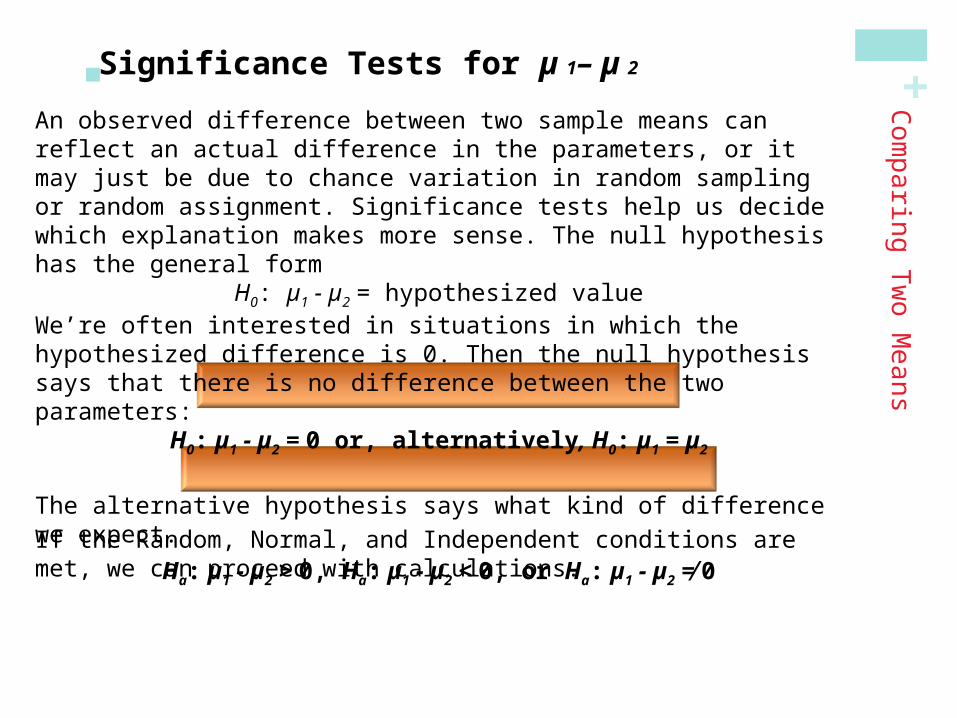
An observed difference between two sample means can reflect an actual difference in the parameters, or it may just be due to chance variation in random sampling or random assignment. Significance tests help us decide which explanation makes more sense. The null hypothesis has the general form

H0: µ1 - µ2 = hypothesized valueWe’re often interested in situations in which the hypothesized difference is 0. Then the null hypothesis says that there is no difference between the twoparameters:

H0: µ1 - µ2 = 0 or, alternatively, H0: µ1 = µ2

The alternative hypothesis says what kind of difference we expect.

Ha: µ1 - µ2 > 0, Ha: µ1 - µ2 < 0, or Ha: µ1 - µ2 ≠ 0

Significance Tests for µ 1 – µ 2C

om

pa

ring

Tw

o M

ean

s

If the Random, Normal, and Independent conditions are met, we can proceed with calculations.

+ Significance Tests for µ 1 – µ 2C

om

pa

ring

Tw

o M

ean

s

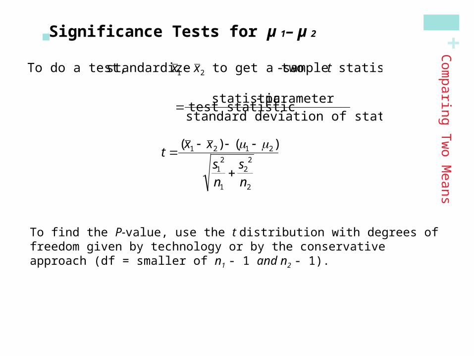
To do a test, standardize x 1 x 2 to get a two- sample t statistic :

test statistic statistic parameter

standard deviation of statistic

t (x 1 x 2) (1 2)

s12

n1

s2

2

n2

To find the P-value, use the t distribution with degrees of freedom given by technology or by the conservative approach (df = smaller of n1 - 1 and n2 - 1).

+ Two-Sample t Test for The Difference Between Two Means If the following conditions are met, we can proceed with a two-sample t

test for the difference between two means:

Co

mp

arin

g T

wo

Mea

ns

Random The data are produced by a random sample of size n1 fromPopulation 1 and a random sample of size n2 from Population 2 or by two groups of size n1 and n2 in a randomized experiment.

Normal Both population distributions (or the true distributions of responses to the two treatments) are Normal OR both sample group sizes are large ( n1 30 and n2 30).

Independent Both the samples or groups themselves and the individualobservations in each sample or group are independent. When samplingwithout replacement, check that the two populations are at least 10 times as large as the corresponding samples (the 10% condition).

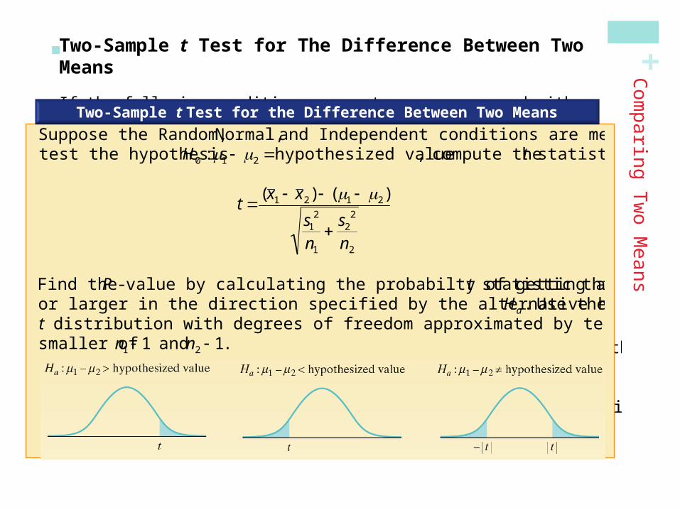
Two-Sample t Test for the Difference Between Two Means

Suppose the Random, Normal, and Independent conditions are met. To test the hypothesis H0 : 1 2 hypothesized value, compute the t statistic

t (x 1 x 2) (1 2)

s12

n1

s2

2

n2

Find the P - value by calculating the probabilty of getting a t statistic this largeor larger in the direction specified by the alternative hypothesis Ha . Use the t distribution with degrees of freedom approximated by technology or thesmaller of n1 1 and n2 1.

+ Example: Calcium and Blood Pressure

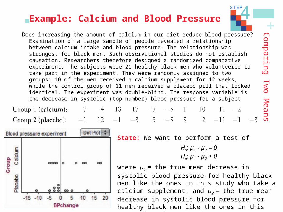
Does increasing the amount of calcium in our diet reduce blood pressure? Examination of a large sample of people revealed a relationship between calcium intake and blood pressure. The relationship was strongest for black men. Such observational studies do not establish causation. Researchers therefore designed a randomized comparative experiment. The subjects were 21 healthy black men who volunteered to take part in the experiment. They were randomly assigned to two groups: 10 of the men received a calcium supplement for 12 weeks, while the control group of 11 men received a placebo pill that looked identical. The experiment was double-blind. The response variable is the decrease in systolic (top number) blood pressure for a subject after 12 weeks, in millimeters of mercury. An increase appears as a negative response Here are the data:

Co

mp

arin

g T

wo

Mea

ns

State: We want to perform a test of

H0: µ1 - µ2 = 0Ha: µ1 - µ2 > 0

where µ1 = the true mean decrease in systolic blood pressure for healthy black men like the ones in this study who take a calcium supplement, and µ2 = the true mean decrease in systolic blood pressure for healthy black men like the ones in this study who take a placebo.We will use α = 0.05.

+ Example: Calcium and Blood PressureC

om

pa

ring

Tw

o M

ean

s

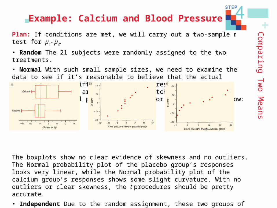
Plan: If conditions are met, we will carry out a two-sample t test for µ1- µ2.

• Random The 21 subjects were randomly assigned to the two treatments.

• Normal With such small sample sizes, we need to examine the data to see if it’s reasonable to believe that the actual distributions of differences in blood pressure when taking calcium or placebo are Normal. Hand sketches of calculator boxplots and Normal probability plots for these data are below:

The boxplots show no clear evidence of skewness and no outliers. The Normal probability plot of the placebo group’s responses looks very linear, while the Normal probability plot of the calcium group’s responses shows some slight curvature. With no outliers or clear skewness, the t procedures should be pretty accurate.

• Independent Due to the random assignment, these two groups of men can be viewed as independent. Individual observations in each group should also be independent: knowing one subject’s change in blood pressure gives no information about another subject’s response.


om

pa

ring

Tw

o M

ean

s

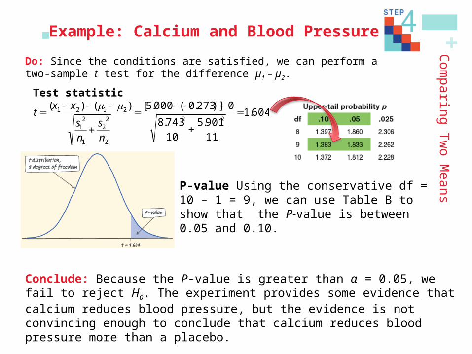
Test statistic :

t (x 1 x 2) (1 2)

s12

n1

s2

2

n2

[5.000 ( 0.273)] 0

8.7432

10 5.9012

11

1.604

Do: Since the conditions are satisfied, we can perform a two-sample t test for the difference µ1 – µ2.

P-value Using the conservative df = 10 – 1 = 9, we can use Table B to show that the P-value is between 0.05 and 0.10.

Conclude: Because the P-value is greater than α = 0.05, we fail to reject H0. The experiment provides some evidence that calcium reduces blood pressure, but the evidence is not convincing enough to conclude that calcium reduces blood pressure more than a placebo.


om

pa

ring

Tw

o M

ean

s

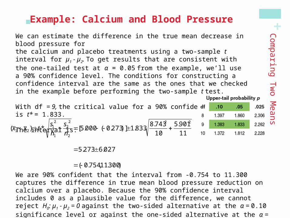
(x 1 x 2) t *s1

2

n1

s2

2

n2

[5.000 ( 0.273)]1.8338.7432

10

5.9012

11

5.2736.027

( 0.754,11.300)

We can estimate the difference in the true mean decrease in blood pressure forthe calcium and placebo treatments using a two-sample t interval for µ1 - µ2. To get results that are consistent with the one-tailed test at α = 0.05 from the example, we’ll use a 90% confidence level. The conditions for constructing a confidence interval are the same as the ones that we checked in the example before performing the two-sample t test.

With df = 9, the critical value for a 90% confidence interval is t* = 1.833.

The interval is:

We are 90% confident that the interval from -0.754 to 11.300 captures the difference in true mean blood pressure reduction on calcium over a placebo. Because the 90% confidence interval includes 0 as a plausible value for the difference, we cannot reject H0: µ1 - µ2 = 0 against the two-sided alternative at the α = 0.10 significance level or against the one-sided alternative at the α = 0.05 significance level.

+ Using Two-Sample t Procedures WiselyC

om

pa

ring

Tw

o M

ean

s

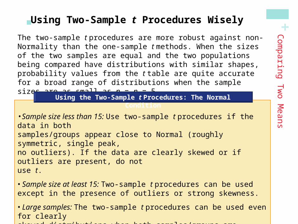
The two-sample t procedures are more robust against non-Normality than the one-sample t methods. When the sizes of the two samples are equal and the two populations being compared have distributions with similar shapes, probability values from the t table are quite accurate for a broad range of distributions when the sample sizes are as small as n1 = n2 = 5.

•Sample size less than 15: Use two-sample t procedures if the data in bothsamples/groups appear close to Normal (roughly symmetric, single peak,no outliers). If the data are clearly skewed or if outliers are present, do notuse t.

• Sample size at least 15: Two-sample t procedures can be used except in the presence of outliers or strong skewness.

• Large samples: The two-sample t procedures can be used even for clearlyskewed distributions when both samples/groups are large, roughly n ≥ 30.

Using the Two-Sample t Procedures: The Normal Condition

+ Using Two-Sample t Procedures WiselyC

om

pa

ring

Tw

o M

ean

s

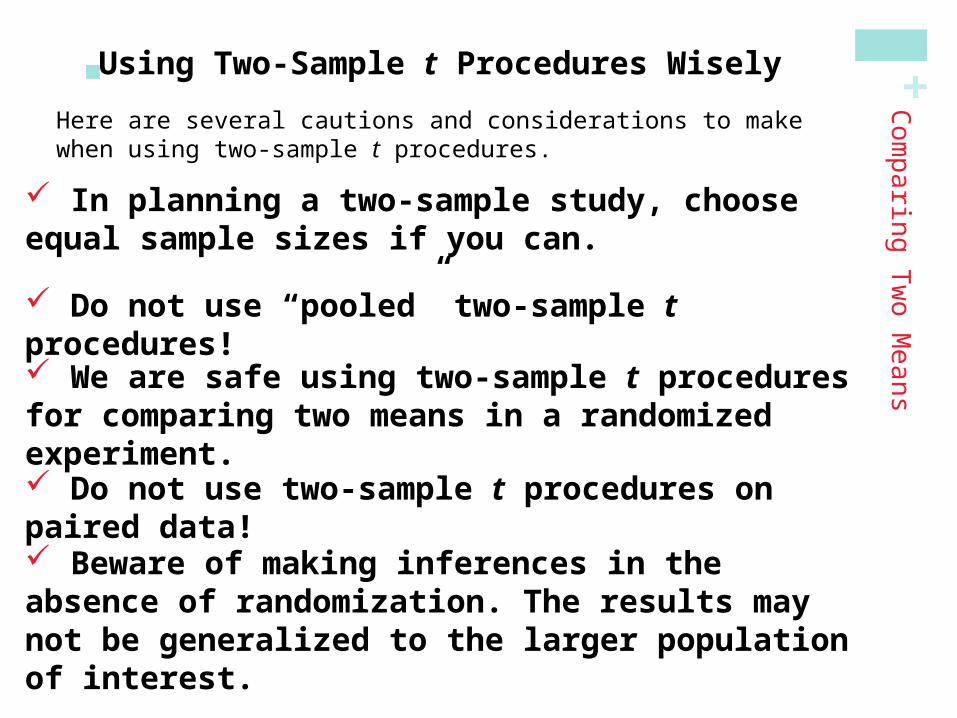
Here are several cautions and considerations to make when using two-sample t procedures.

In planning a two-sample study, choose equal sample sizes if you can.

Do not use “pooled” two-sample t procedures!

We are safe using two-sample t procedures for comparing two means in a randomized experiment.

Do not use two-sample t procedures on paired data!

Beware of making inferences in the absence of randomization. The results may not be generalized to the larger population of interest.


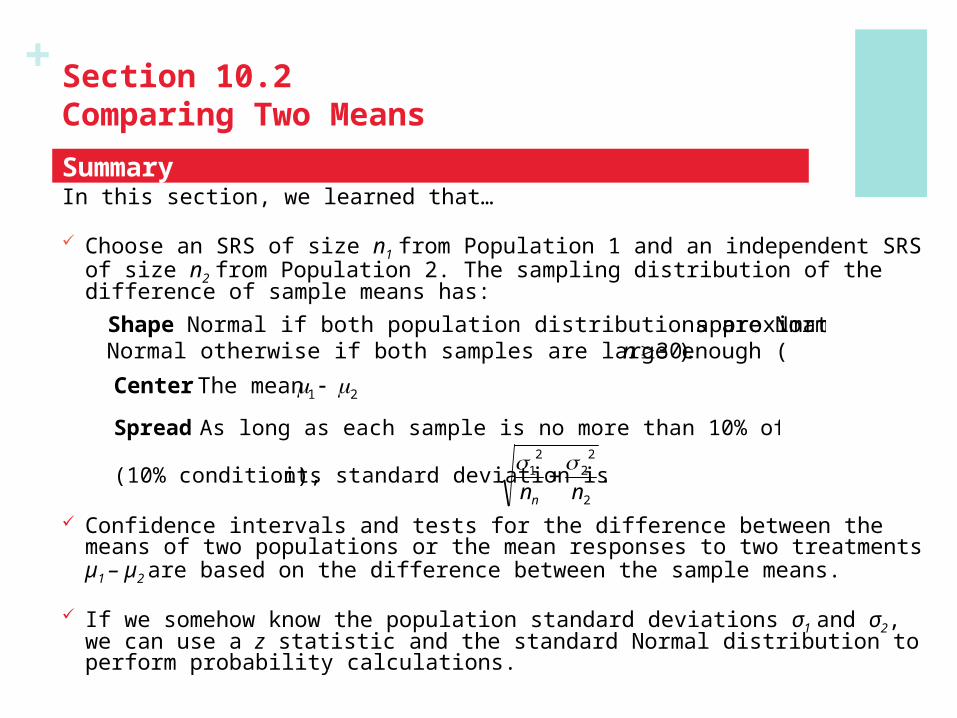
In this section, we learned that…

Choose an SRS of size n1 from Population 1 and an independent SRS of size n2 from Population 2. The sampling distribution of the difference of sample means has:

Confidence intervals and tests for the difference between the means of two populations or the mean responses to two treatments µ1 – µ2 are based on the difference between the sample means.

If we somehow know the population standard deviations σ1 and σ2, we can use a z statistic and the standard Normal distribution to perform probability calculations.

Summary

Center The mean 1 2.

Shape Normal if both population distributions are Normal; approximately Normal otherwise if both samples are large enough ( n 30).

Spread As long as each sample is no more than 10% of its population

(10% condition), its standard deviation is1

2

nn

22

n2

.


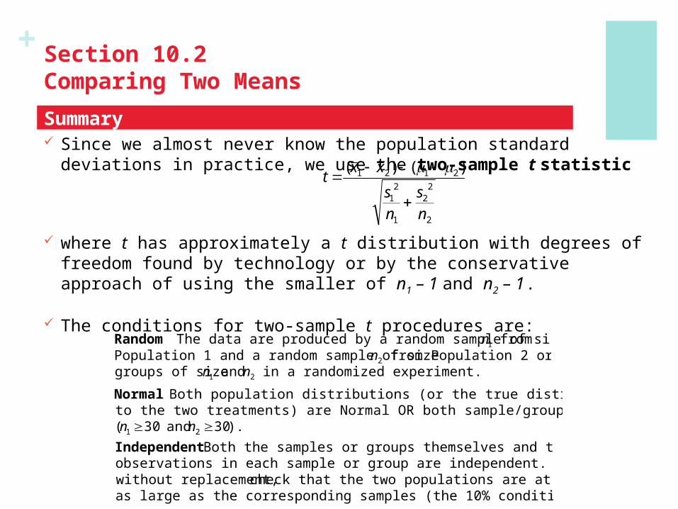
Since we almost never know the population standard deviations in practice, we use the two-sample t statistic

where t has approximately a t distribution with degrees of freedom found by technology or by the conservative approach of using the smaller of n1 – 1 and n2 – 1 .

The conditions for two-sample t procedures are:

Summary

Random The data are produced by a random sample of size n1 fromPopulation 1 and a random sample of size n2 from Population 2 or by twogroups of size n1 and n2 in a randomized experiment.

Normal Both population distributions (or the true distributions of responsesto the two treatments) are Normal OR both sample/group sizes are large(n1 30 and n2 30).

Independent Both the samples or groups themselves and the individualobservations in each sample or group are independent. When samplingwithout replacement, check that the two populations are at least 10 timesas large as the corresponding samples (the 10% condition).

t (x 1 x 2) (1 2)

s12

n1

s2

2

n2


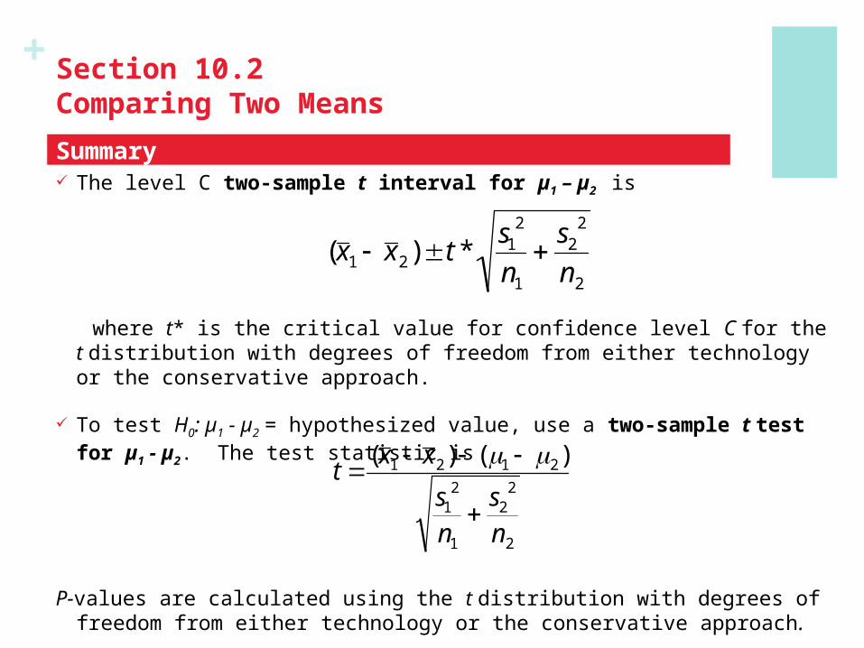
The level C two-sample t interval for µ1 – µ2 is

where t* is the critical value for confidence level C for the t distribution with degrees of freedom from either technology or the conservative approach.

To test H0: µ1 - µ2 = hypothesized value, use a two-sample t test for µ1 - µ2. The test statistic is

P-values are calculated using the t distribution with degrees of freedom from either technology or the conservative approach.

Summary

(x 1 x 2) t *s1

2

n1

s2

2

n2

t (x 1 x 2) (1 2)

s12

n1

s2

2

n2


The two-sample t procedures are quite robust against departures from Normality, especially when both sample/group sizes are large.

Inference about the difference µ1 - µ2 in the effectiveness of two treatments in a completely randomized experiment is based on the randomization distribution of the difference between sample means. When the Random, Normal, and Independent conditions are met, our usual inference procedures based on the sampling distribution of the difference between sample means will be approximately correct.

Don’t use two-sample t procedures to compare means for paired data.

Summary

+Looking Ahead…

We’ll learn how to perform inference for distributions of categorical data.

We’ll learn about Chi-square Goodness-of-Fit tests Inference for Relationships

In the next Chapter…

+ Comparing Two Means Introduction In the previous section, we developed methods for comparing two...

Documents

Transcript of + Comparing Two Means Introduction In the previous section, we developed methods for comparing two...