© Boardworks Ltd 20051 of 33 © Boardworks Ltd 2005 1 of 33 AS-Level Maths: Statistics 1 for...

© Boardworks Ltd 20051 of 33 © Boardworks Ltd 20051 of 33

AS-Level Maths: Statistics 1for Edexcel

S1.6 The normal distribution

This icon indicates the slide contains activities created in Flash. These activities are not editable.

For more detailed instructions, see the Getting Started presentation.

© Boardworks Ltd 20052 of 33

Co

nte

nts


Introduction: Normal distribution


The standard normal distribution

More general normal distributions

Solving problems by working backwards


Histogram showing the heights of 10000 males

0

200

400

600

800

1000

1200

1400

140 148 156 164 172 180 188 More

Height (cm)

Fre

qu

ency

A sample of heights of 10,000 adult males gave rise to the following histogram:

Notice that this histogram is symmetrical and bell-shaped. This is the characteristic

shape of a normal distribution.



The normal distribution is an appropriate model for many common continuous distributions, for example:

If we were to draw a smooth curve through the mid-points of the bars in the histogram of these heights, it would have the following shape:


This is called the normal curve.

The masses of new-born babies;

The IQs of school students;

The hand span of adult females;

The heights of plants growing in a field;etc.


All normal curves are symmetrical and bell-shaped but the exact shape is governed by 2 parameters – the mean, μ, and the standard deviation, σ.



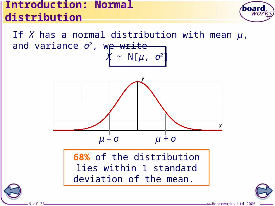
If X has a normal distribution with mean μ, and variance σ2, we write

X ~ N[μ, σ2]

68% of the distribution lies within 1 standard deviation of the mean.


x

y

μ – σ μ + σ


95% of the distribution lies within 2 standard deviations of the mean.


x

y


X ~ N[μ, σ2]

μ – 2σ μ + 2σ


99.7% of the distribution lies within 3 standard deviations of the mean.


x

y


X ~ N[μ, σ2]

μ + 3σμ – 3σ


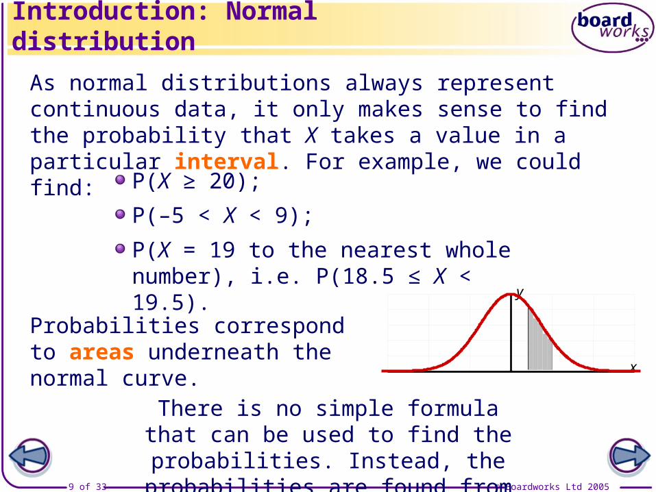
As normal distributions always represent continuous data, it only makes sense to find the probability that X takes a value in a particular interval. For example, we could find:


There is no simple formula that can be used to find the probabilities. Instead, the

probabilities are found from tables.

Probabilities correspond to areas underneath the normal curve.

P(X ≥ 20);

P(–5 < X < 9);

P(X = 19 to the nearest whole number), i.e. P(18.5 ≤ X < 19.5).

x

y


Co

nte

nts








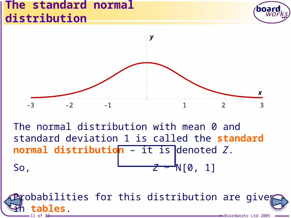
The normal distribution with mean 0 and standard deviation 1 is called the standard normal distribution – it is denoted Z.

So, Z ~ N[0, 1]

Probabilities for this distribution are given in tables.


-3 -2 -1 1 2 3

x

y


Here is an extract from a standard normal distribution table:

z 0 1 2 3 4 5 6 7 8 9

0.0 .5000 .5040 .5080 .5120 .5160 .5199 .5239 .5279 .5319 .5359

0.1 .5398 .5438 .5478 .5517 .5557 .5596 .5636 .5675 .5714 .5753

0.2 .5793 .5832 .5871 .5910 .5948 .5987 .6026 .6064 .6103 .6141

0.3 .6179 .6217 .6255 .6293 .6331 .6368 .6406 .6443 .6480 .6517

0.4 .6554 .6591 .6628 .6664 .6700 .6736 .6772 .6808 .6844 .6879

0.5 .6915 .6950 .6985 .7019 .7054 .7088 .7123 .7157 .7190 .7224

0.6 .7257 .7291 .7324 .7357 .7389 .7422 .7454 .7486 .7517 .7549

0.7 .7580 .7611 .7642 .7673 .7704 .7734 .7764 .7794 .7823 .7852

0.8 .7881 .7910 .7939 .7967 .7995 .8023 .8051 .8078 .8106 .8133

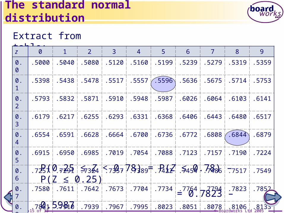
The tables are cumulative, i.e. they give P(Z ≤ z).


This column gives the first part of the z value.This row gives the next decimal place of the z value.


So, P(Z ≤ 0.54) = 0.7054.


Extract from table:

z 0 1 2 3 4 5 6 7 8 9

0.0 .5000 .5040 .5080 .5120 .5160 .5199 .5239 .5279 .5319 .5359

0.1 .5398 .5438 .5478 .5517 .5557 .5596 .5636 .5675 .5714 .5753

0.2 .5793 .5832 .5871 .5910 .5948 .5987 .6026 .6064 .6103 .6141

0.3 .6179 .6217 .6255 .6293 .6331 .6368 .6406 .6443 .6480 .6517

0.4 .6554 .6591 .6628 .6664 .6700 .6736 .6772 .6808 .6844 .6879

0.5 .6915 .6950 .6985 .7019 .7054 .7088 .7123 .7157 .7190 .7224

0.6 .7257 .7291 .7324 .7357 .7389 .7422 .7454 .7486 .7517 .7549

0.7 .7580 .7611 .7642 .7673 .7704 .7734 .7764 .7794 .7823 .7852

0.8 .7881 .7910 .7939 .7967 .7995 .8023 .8051 .8078 .8106 .8133


P(Z > 0.6) = 1 – P(Z ≤ 0.6)

= 1 – 0.7257

= 0.2743


Extract from table:

z 0 1 2 3 4 5 6 7 8 9

0.0 .5000 .5040 .5080 .5120 .5160 .5199 .5239 .5279 .5319 .5359

0.1 .5398 .5438 .5478 .5517 .5557 .5596 .5636 .5675 .5714 .5753

0.2 .5793 .5832 .5871 .5910 .5948 .5987 .6026 .6064 .6103 .6141

0.3 .6179 .6217 .6255 .6293 .6331 .6368 .6406 .6443 .6480 .6517

0.4 .6554 .6591 .6628 .6664 .6700 .6736 .6772 .6808 .6844 .6879

0.5 .6915 .6950 .6985 .7019 .7054 .7088 .7123 .7157 .7190 .7224

0.6 .7257 .7291 .7324 .7357 .7389 .7422 .7454 .7486 .7517 .7549

0.7 .7580 .7611 .7642 .7673 .7704 .7734 .7764 .7794 .7823 .7852

0.8 .7881 .7910 .7939 .7967 .7995 .8023 .8051 .8078 .8106 .8133


P(0.25 ≤ Z < 0.78) = P(Z ≤ 0.78) – P(Z ≤ 0.25)

= 0.7823 – 0.5987

= 0.1836


Extract from table:

z 0 1 2 3 4 5 6 7 8 9

0.0 .5000 .5040 .5080 .5120 .5160 .5199 .5239 .5279 .5319 .5359

0.1 .5398 .5438 .5478 .5517 .5557 .5596 .5636 .5675 .5714 .5753

0.2 .5793 .5832 .5871 .5910 .5948 .5987 .6026 .6064 .6103 .6141

0.3 .6179 .6217 .6255 .6293 .6331 .6368 .6406 .6443 .6480 .6517

0.4 .6554 .6591 .6628 .6664 .6700 .6736 .6772 .6808 .6844 .6879

0.5 .6915 .6950 .6985 .7019 .7054 .7088 .7123 .7157 .7190 .7224

0.6 .7257 .7291 .7324 .7357 .7389 .7422 .7454 .7486 .7517 .7549

0.7 .7580 .7611 .7642 .7673 .7704 .7734 .7764 .7794 .7823 .7852

0.8 .7881 .7910 .7939 .7967 .7995 .8023 .8051 .8078 .8106 .8133


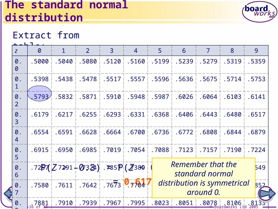
P(Z > –0.3) = P(Z < 0.3)

= 0.6179


Extract from table:

z 0 1 2 3 4 5 6 7 8 9

0.0 .5000 .5040 .5080 .5120 .5160 .5199 .5239 .5279 .5319 .5359

0.1 .5398 .5438 .5478 .5517 .5557 .5596 .5636 .5675 .5714 .5753

0.2 .5793 .5832 .5871 .5910 .5948 .5987 .6026 .6064 .6103 .6141

0.3 .6179 .6217 .6255 .6293 .6331 .6368 .6406 .6443 .6480 .6517

0.4 .6554 .6591 .6628 .6664 .6700 .6736 .6772 .6808 .6844 .6879

0.5 .6915 .6950 .6985 .7019 .7054 .7088 .7123 .7157 .7190 .7224

0.6 .7257 .7291 .7324 .7357 .7389 .7422 .7454 .7486 .7517 .7549

0.7 .7580 .7611 .7642 .7673 .7704 .7734 .7764 .7794 .7823 .7852

0.8 .7881 .7910 .7939 .7967 .7995 .8023 .8051 .8078 .8106 .8133

Remember that the standard normal distribution

is symmetrical around 0.


P(Z ≤ –0.28) = 1 – P(Z ≤ 0.28)

= 1 – 0.6103

= 0.3897


Extract from table:

z 0 1 2 3 4 5 6 7 8 9

0.0 .5000 .5040 .5080 .5120 .5160 .5199 .5239 .5279 .5319 .5359

0.1 .5398 .5438 .5478 .5517 .5557 .5596 .5636 .5675 .5714 .5753

0.2 .5793 .5832 .5871 .5910 .5948 .5987 .6026 .6064 .6103 .6141

0.3 .6179 .6217 .6255 .6293 .6331 .6368 .6406 .6443 .6480 .6517

0.4 .6554 .6591 .6628 .6664 .6700 .6736 .6772 .6808 .6844 .6879

0.5 .6915 .6950 .6985 .7019 .7054 .7088 .7123 .7157 .7190 .7224

0.6 .7257 .7291 .7324 .7357 .7389 .7422 .7454 .7486 .7517 .7549

0.7 .7580 .7611 .7642 .7673 .7704 .7734 .7764 .7794 .7823 .7852

0.8 .7881 .7910 .7939 .7967 .7995 .8023 .8051 .8078 .8106 .8133


P(–0.08 < Z ≤ 0.85) = P(Z ≤ 0.85) – P(Z ≤ –0.08)

= 0.8023 – (1 – 0.5319)

= 0.3342


Extract from table:

z 0 1 2 3 4 5 6 7 8 9

0.0 .5000 .5040 .5080 .5120 .5160 .5199 .5239 .5279 .5319 .5359

0.1 .5398 .5438 .5478 .5517 .5557 .5596 .5636 .5675 .5714 .5753

0.2 .5793 .5832 .5871 .5910 .5948 .5987 .6026 .6064 .6103 .6141

0.3 .6179 .6217 .6255 .6293 .6331 .6368 .6406 .6443 .6480 .6517

0.4 .6554 .6591 .6628 .6664 .6700 .6736 .6772 .6808 .6844 .6879

0.5 .6915 .6950 .6985 .7019 .7054 .7088 .7123 .7157 .7190 .7224

0.6 .7257 .7291 .7324 .7357 .7389 .7422 .7454 .7486 .7517 .7549

0.7 .7580 .7611 .7642 .7673 .7704 .7734 .7764 .7794 .7823 .7852

0.8 .7881 .7910 .7939 .7967 .7995 .8023 .8051 .8078 .8106 .8133


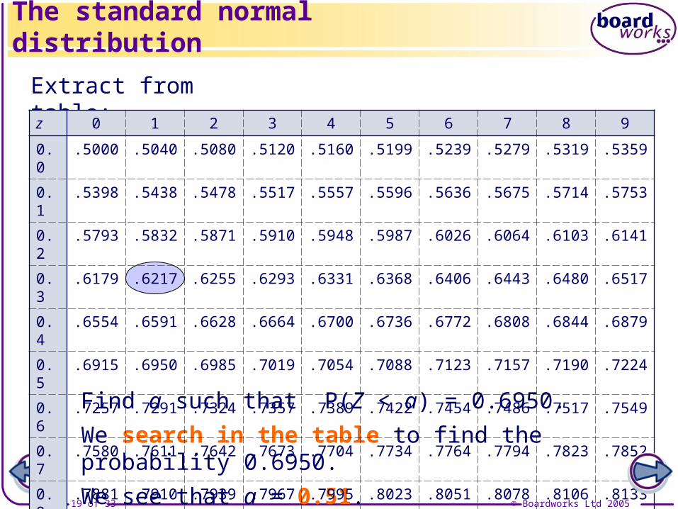
Find a such that P(Z < a) = 0.6950.

We search in the table to find the probability 0.6950.

We see that a = 0.51.


Extract from table:

z 0 1 2 3 4 5 6 7 8 9

0.0 .5000 .5040 .5080 .5120 .5160 .5199 .5239 .5279 .5319 .5359

0.1 .5398 .5438 .5478 .5517 .5557 .5596 .5636 .5675 .5714 .5753

0.2 .5793 .5832 .5871 .5910 .5948 .5987 .6026 .6064 .6103 .6141

0.3 .6179 .6217 .6255 .6293 .6331 .6368 .6406 .6443 .6480 .6517

0.4 .6554 .6591 .6628 .6664 .6700 .6736 .6772 .6808 .6844 .6879

0.5 .6915 .6950 .6985 .7019 .7054 .7088 .7123 .7157 .7190 .7224

0.6 .7257 .7291 .7324 .7357 .7389 .7422 .7454 .7486 .7517 .7549

0.7 .7580 .7611 .7642 .7673 .7704 .7734 .7764 .7794 .7823 .7852

0.8 .7881 .7910 .7939 .7967 .7995 .8023 .8051 .8078 .8106 .8133


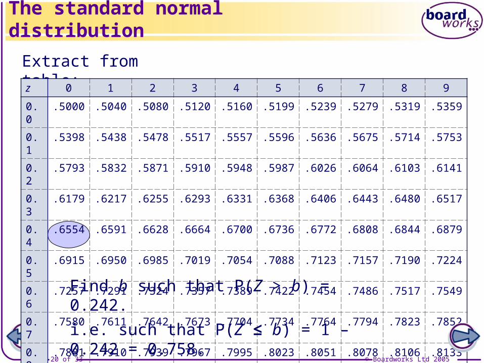
Find b such that P(Z > b) = 0.242.

i.e. such that P(Z ≤ b) = 1 – 0.242 = 0.758.

We see that b = 0.7.


Extract from table:

z 0 1 2 3 4 5 6 7 8 9

0.0 .5000 .5040 .5080 .5120 .5160 .5199 .5239 .5279 .5319 .5359

0.1 .5398 .5438 .5478 .5517 .5557 .5596 .5636 .5675 .5714 .5753

0.2 .5793 .5832 .5871 .5910 .5948 .5987 .6026 .6064 .6103 .6141

0.3 .6179 .6217 .6255 .6293 .6331 .6368 .6406 .6443 .6480 .6517

0.4 .6554 .6591 .6628 .6664 .6700 .6736 .6772 .6808 .6844 .6879

0.5 .6915 .6950 .6985 .7019 .7054 .7088 .7123 .7157 .7190 .7224

0.6 .7257 .7291 .7324 .7357 .7389 .7422 .7454 .7486 .7517 .7549

0.7 .7580 .7611 .7642 .7673 .7704 .7734 .7764 .7794 .7823 .7852

0.8 .7881 .7910 .7939 .7967 .7995 .8023 .8051 .8078 .8106 .8133


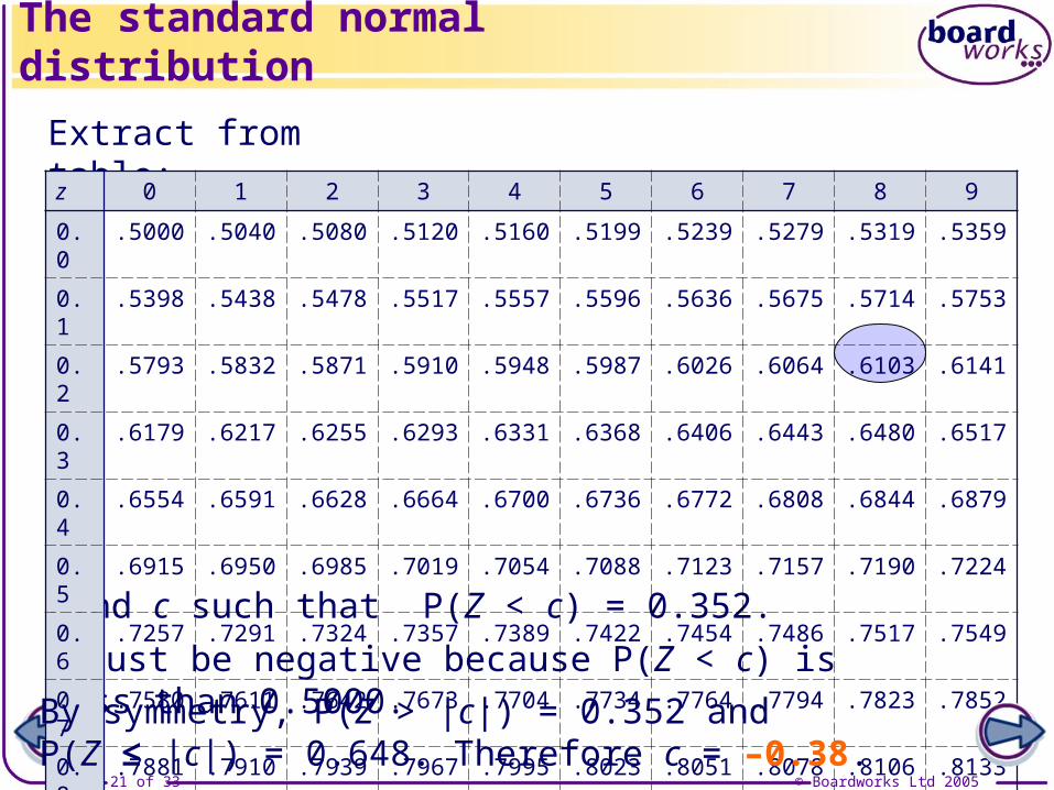
Find c such that P(Z < c) = 0.352.

c must be negative because P(Z < c) is less than 0.5000.


Extract from table:

z 0 1 2 3 4 5 6 7 8 9

0.0 .5000 .5040 .5080 .5120 .5160 .5199 .5239 .5279 .5319 .5359

0.1 .5398 .5438 .5478 .5517 .5557 .5596 .5636 .5675 .5714 .5753

0.2 .5793 .5832 .5871 .5910 .5948 .5987 .6026 .6064 .6103 .6141

0.3 .6179 .6217 .6255 .6293 .6331 .6368 .6406 .6443 .6480 .6517

0.4 .6554 .6591 .6628 .6664 .6700 .6736 .6772 .6808 .6844 .6879

0.5 .6915 .6950 .6985 .7019 .7054 .7088 .7123 .7157 .7190 .7224

0.6 .7257 .7291 .7324 .7357 .7389 .7422 .7454 .7486 .7517 .7549

0.7 .7580 .7611 .7642 .7673 .7704 .7734 .7764 .7794 .7823 .7852

0.8 .7881 .7910 .7939 .7967 .7995 .8023 .8051 .8078 .8106 .8133

By symmetry, P(Z > |c|) = 0.352 and P(Z ≤ |c|) = 0.648. Therefore c = –0.38.


Co

nte

nts








It would of course be impractical to publish tables of probabilities for every possible normal distribution.

Fortunately, it is possible and easy to transform any normal distribution to a standard normal:

If X ~ then ~ [ ].N 0,1X

Z

[ , ]2N

Standardize

[ ]N 0, 1


x

y[ , ]2N

-3 -2 -1 1 2 3

x

y


Example: If , find

a) P(X < 23);

b) P(X > 14);

c) P(16 < X < 24.8).

~ [ , ]N 20 16X

a) If σ2 = 16, then σ = 4.

( ) ( . )P 23 P 0 75X Z


x

y

x

y

20 23 0 0.75

Standardize

.23 20

0 754

= 0.7734


b)

( ) ( . ) ( . )P 14 P 1 5 P 1 5X Z Z


Example: If , find

a) P(X < 23);

b) P(X > 14);

c) P(16 < X < 24.8).

~ [ , ]N 20 16X

x

y

x

y

14 20 –1.5 0

Standardize

.14 20

1 54

= 0.9332


c) .. ( . )

16 20 24 8 20P 16 24 8 P P 1 1 2

4 4X Z Z

P(Z < 1.2) = 0.8849

and P(Z < –1) = 1 – P(Z < 1) = 1 – 0.8413 = 0.1587.

So, P(–1 < Z < 1.2) = 0.8849 – 0.1587 = 0.7262


Example: If , find

a) P(X < 23);

b) P(X > 14);

c) P(16 < X < 24.8).

~ [ , ]N 20 16X

x

y

x

y

Standardize

16 20 24.8 -1 0 1.2


Let X be the random variable for the IQ of an individual.X ~ N[100, 225].

So, we want P(X > 124) = P(Z > 1.6)

= 1 – P(Z ≤ 1.6) = 1 – 0.9452


Examination-style question: IQs are normally distributed with mean 100 and standard deviation 15. What proportion of the population have an IQ of at least 124?

x

y

x

y

100 124 0 1.6

Standardize

.124 100

1 615

= 0.0548


Co

nte

nts






Working backwards


x

y

To find x, we start by finding the standardized value z such that P(Z < z) = 0.67.

From tables we see that z = 0.44.

We therefore need to find the value that standardizes to make 0.44 by rearranging the formula.

Example: If X ~ N[4, 0.25], find the value of x if P(X < x) = 0.67.

Working backwards

x

y

4 x 0 0.44

Standardize

[ . ]N 4, 0 25 [ ]N 0, 1.

.

.4 0 44 0

4 22

5x

x


x

y

x

y

Let X represent the marks in the examination. X ~ N[62, 256].

We need to find x such that P(X ≥ x) = 0.86.

We need to solve: . Therefore x = 44.72.

Example: Marks in an examination can be assumed to follow a normal distribution with mean 62 and standard deviation 16. The pass mark is to be chosen so that 86% of candidates pass. Find the pass mark.

–1.08

.62

1 0816

x

x

Working backwards

Standardize

So, the pass mark is 44.


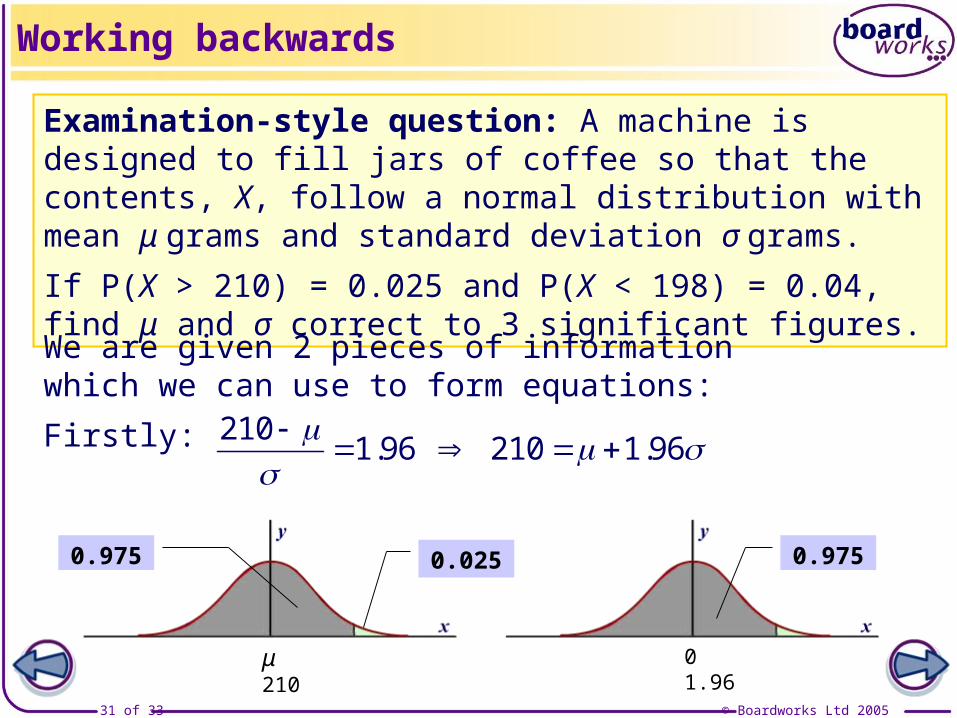
Examination-style question: A machine is designed to fill jars of coffee so that the contents, X, follow a normal distribution with mean μ grams and standard deviation σ grams.

If P(X > 210) = 0.025 and P(X < 198) = 0.04, find μ and σ correct to 3 significant figures.

μ 210

0.975

0 1.96

. .210

1 96 210 1 96

0.025

Working backwards

We are given 2 pieces of information which we can use to form equations:

Firstly:

0.975


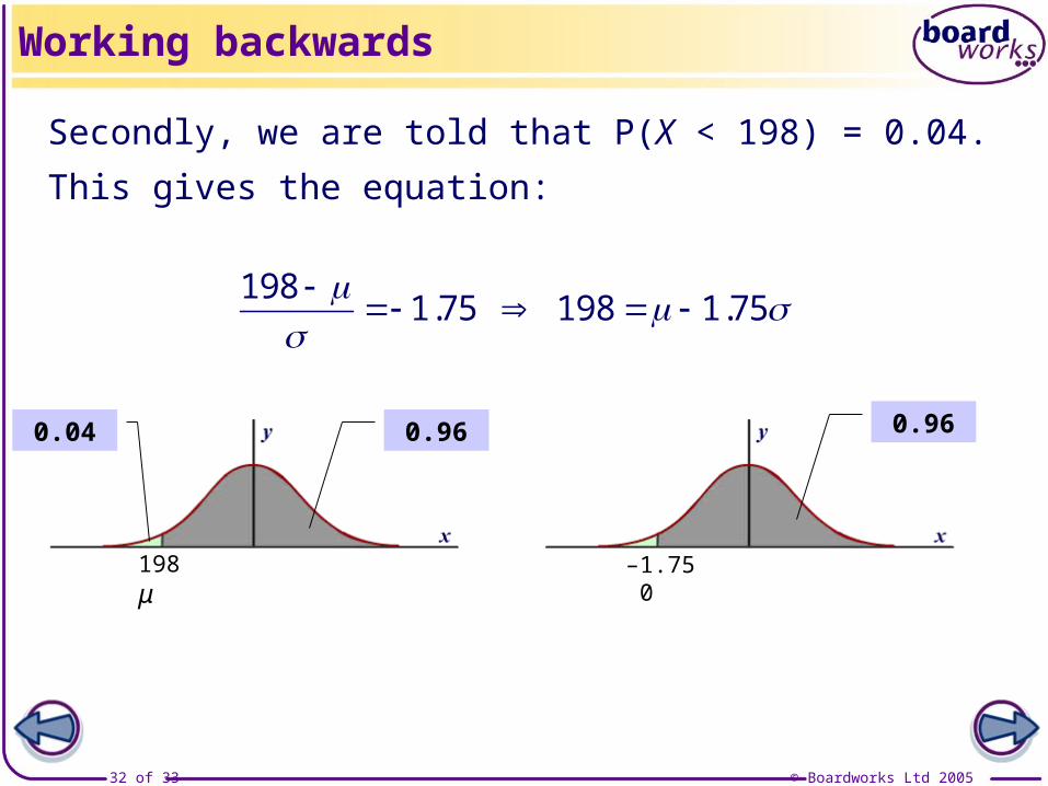
Secondly, we are told that P(X < 198) = 0.04.

This gives the equation:

198 μ

0.04

–1.75 0

. .198

1 75 198 1 75

0.96

Working backwards

0.96


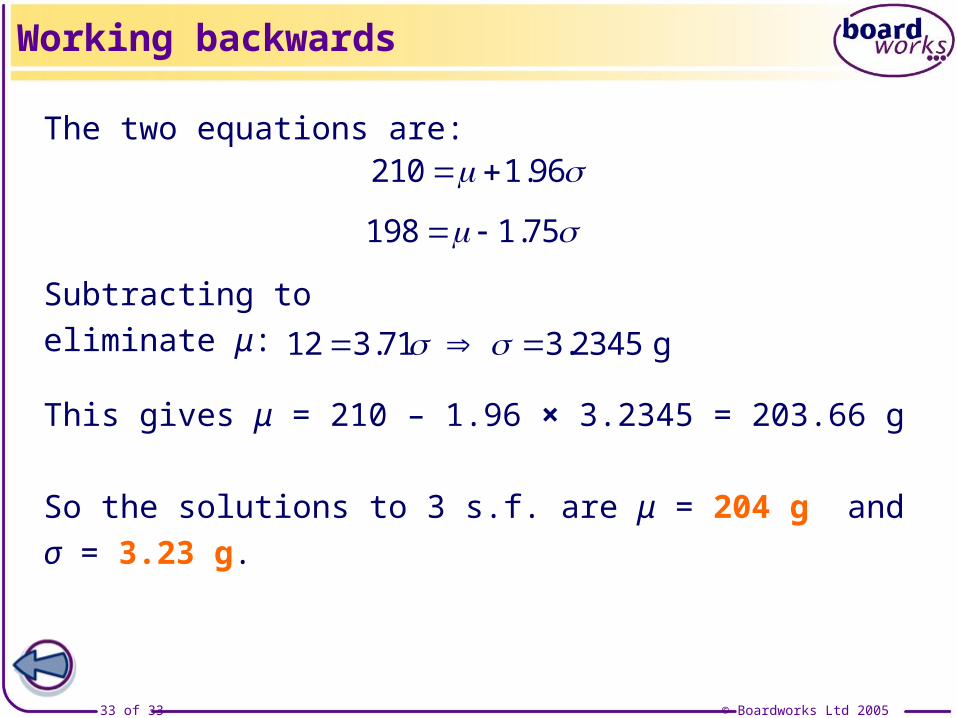
The two equations are:

.198 1 75

.210 1 96

Subtracting to eliminate μ:

. .12 3 71 3 2345 g

This gives μ = 210 – 1.96 × 3.2345 = 203.66 g

So the solutions to 3 s.f. are μ = 204 g and σ = 3.23 g.

Working backwards

© Boardworks Ltd 20051 of 33 © Boardworks Ltd 2005 1 of 33 AS-Level Maths: Statistics 1 for...

Documents

Transcript of © Boardworks Ltd 20051 of 33 © Boardworks Ltd 2005 1 of 33 AS-Level Maths: Statistics 1 for...