Hypothesis Tests: Two Independent Samples Cal State Northridge 320 Andrew Ainsworth PhD.
date post
21-Dec-2015Category
view
222download
0
320
Ainsworth
One-way Between Groups Analysis of Variance

Psy 320 - Cal State Northridge 2
Major Points
Problem with t-tests and multiple groups
The logic behind ANOVA
Calculations
Multiple comparisons
Assumptions of analysis of variance
Effect Size for ANOVA
Psy 320 - Cal State Northridge 3
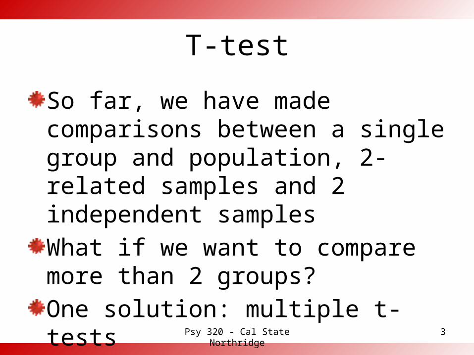
T-test
So far, we have made comparisons between a single group and population, 2-related samples and 2 independent samples
What if we want to compare more than 2 groups?
One solution: multiple t-tests
Psy 320 - Cal State Northridge 4
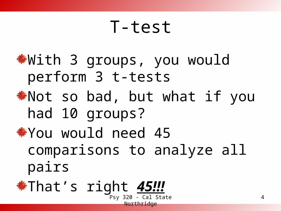
T-test
With 3 groups, you would perform 3 t-tests
Not so bad, but what if you had 10 groups?
You would need 45 comparisons to analyze all pairs
That’s right 45!!!
Psy 320 - Cal State Northridge 5
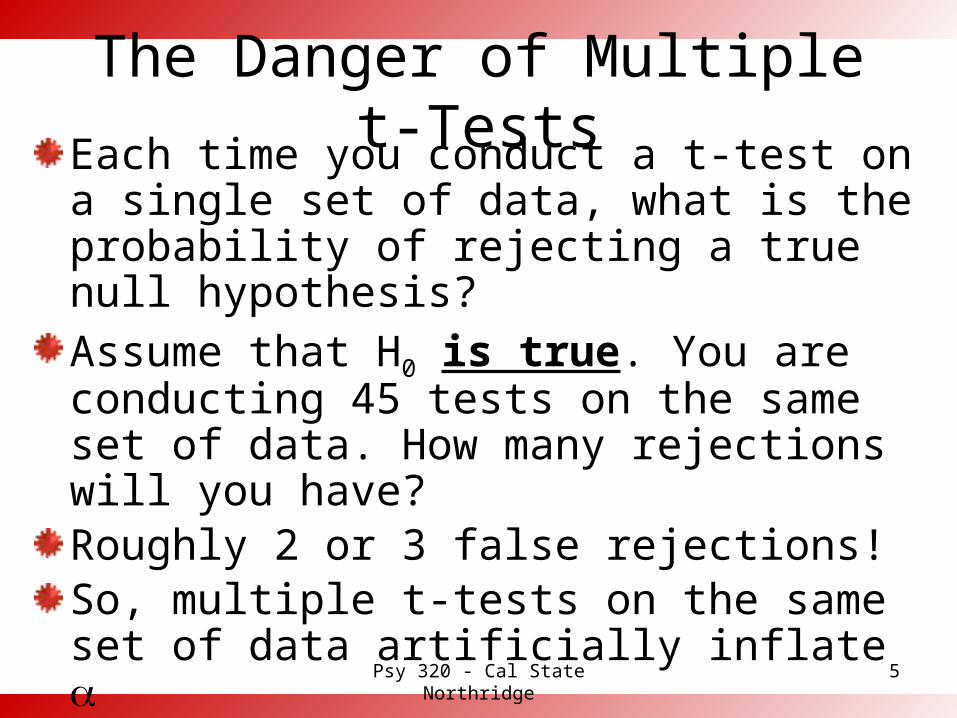
The Danger of Multiple t-TestsEach time you conduct a t-test on a single set of data, what is the probability of rejecting a true null hypothesis?
Assume that H0 is true. You are conducting 45 tests on the same set of data. How many rejections will you have?Roughly 2 or 3 false rejections!So, multiple t-tests on the same set of data artificially inflate

Psy 320 - Cal State Northridge 6
Summary: The Problems With Multiple t-Tests
Inefficient - too many comparisons when we have even modest numbers of groups.
Imprecise - cannot discern patterns or trends of differences in subsets of groups.
Inaccurate - multiple tests on the same set of data artificially inflate What is needed: a single test for the overall difference among all means
e.g. ANOVA

Psy 320 - Cal State Northridge
LOGIC OF THE ANALYSIS OF VARIANCE
7

Psy 320 - Cal State Northridge 8
Logic of the Analysis of Variance
Null hypothesis h0: Population means equalm1 = m2 = m3 = m4
Alternative hypothesis: h1 –Not all population means equal.

Psy 320 - Cal State Northridge 9
Logic
Create a measure of variability among group means–MSBetweenGroups AKA s2
BetweenGroups
Create a measure of variability within groups–MSWithinGroups AKA s2
WithinGroups

Psy 320 - Cal State Northridge 10
Logic
MSBetweenGroups /MSWithinGroups –Ratio approximately 1 if null true–Ratio significantly larger than 1 if null
false– “approximately 1” can actually be as
high as 2 or 3, but not much higher

Psy 320 - Cal State Northridge 11
“So, why is it called analysis of variance anyway?”
Aren’t we interested in mean differences?
Variance revisited–Basic variance formula
2
2
1iX X SS
sn df

Psy 320 - Cal State Northridge 12
“Why is it called analysis of variance anyway?”
What if data comes from groups?– We can have different sums of squares
2
1
2
2
2
3
Where represents the individual,
represents the groups and
GM represent the ungrouped (grand) mean
i GM
i j
j j GM
SS Y Y
SS Y Y
SS n Y Y
i
j

Psy 320 - Cal State Northridge 13
Y-A
xis
X-Axis
3GroupY1GroupY 2GroupYJohn’s Score
X
Grand Mean(Ungrouped Mean)
Logic of ANOVA

Psy 320 - Cal State Northridge
CALCULATIONS
14

Psy 320 - Cal State Northridge 15
Sums of Squares
The total variability can be partitioned into between groups variability and within groups variability.
2 22
i GM j j GM i j
Total BetweenGroups WithinGroups
T BG WG
T Effect Error
Y Y n Y Y Y Y
SS SS SS
SS SS SS
SS SS SS
Psy 320 - Cal State Northridge 16
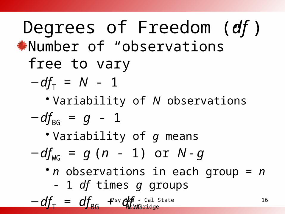
Degrees of Freedom (df )Number of “observations” free to vary–dfT = N - 1
• Variability of N observations
–dfBG = g - 1• Variability of g means
–dfWG = g (n - 1) or N - g• n observations in each group = n - 1 df
times g groups
–dfT = dfBG + dfWG
Psy 320 - Cal State Northridge 17
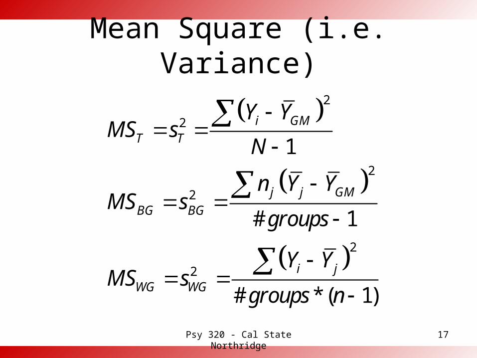
Mean Square (i.e. Variance)
2
2
2
2
2
2
1
# 1
# *( 1)
i GM
T T
j j GM
BG BG
i j
WG WG
Y YMS s
N
n Y YMS s
groups
Y YMS s
groups n

Psy 320 - Cal State Northridge 18
F-test
MSWG contains random sampling variation among the participants
MSBG also contains random sampling variation but it can also contain systematic (real) variation between the groups (either naturally occurring or manipulated)
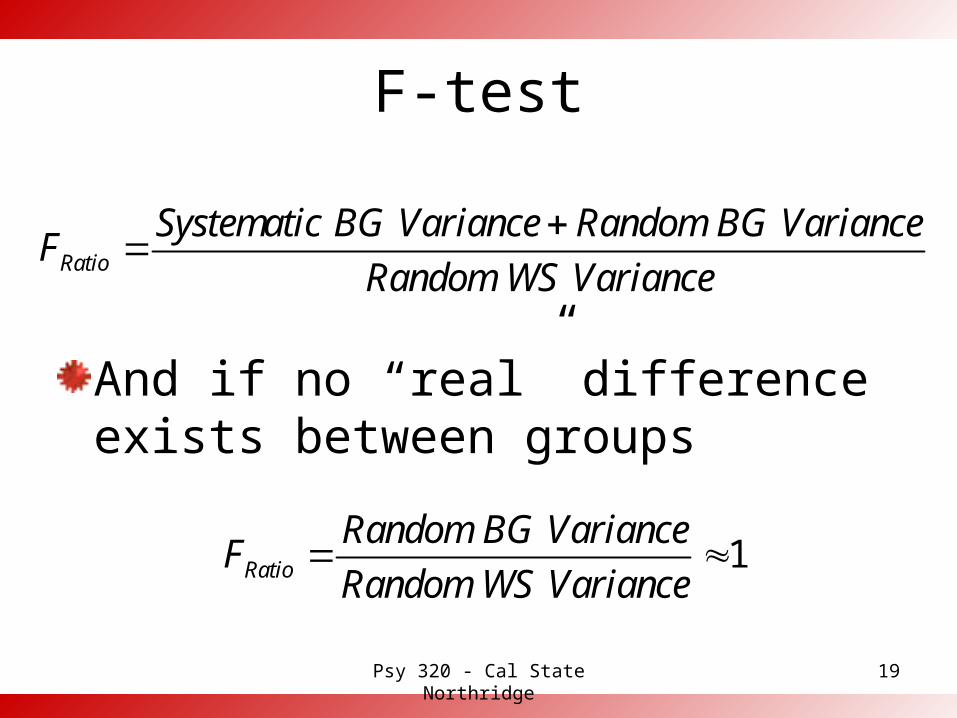
Psy 320 - Cal State Northridge 19
F-test
And if no “real” difference exists between groups
Ratio
Systematic BG Variance Random BG VarianceF
Random WS Variance
1
Ratio
Random BG VarianceF
Random WS Variance

Psy 320 - Cal State Northridge 20
F-test
The F-test is a ratio of the MSBG/MSWG and if the group differences are just random the ratio will equal 1 (e.g. random/random)
Y-A
xis
X-Axis
Y
Grand Mean(Ungrouped Mean)
Y Y
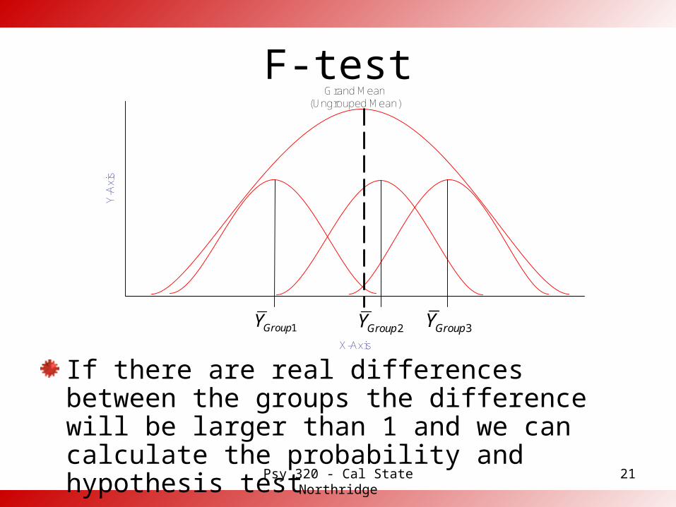
Psy 320 - Cal State Northridge 21
F-testY
-Axi
s
X-Axis
3GroupY1GroupY 2GroupY
Grand Mean(Ungrouped Mean)
If there are real differences between the groups the difference will be larger than 1 and we can calculate the probability and hypothesis test
Psy 320 - Cal State Northridge 22
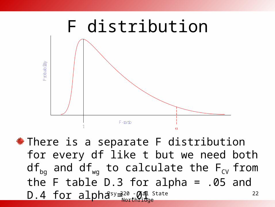
F distributionP
roba
bilit
y
F-ratio1 a
There is a separate F distribution for every df like t but we need both dfbg and dfwg to calculate the FCV from the F table D.3 for alpha = .05 and D.4 for alpha = .01

Psy 320 - Cal State Northridge
1-WAY BETWEEN GROUPS ANOVA EXAMPLE
23
Psy 320 - Cal State Northridge 24
ExampleA researcher is interested in knowing which brand of baby food babies prefer: Beechnut, Del Monte or Gerber.
He randomly selects 15 babies and assigns each to try strained peas from one of the three brands
Liking is measured by the number of spoonfuls the baby takes before getting “upset” (e.g. crying, screaming, throwing the food, etc.)

Psy 320 - Cal State Northridge 25
Hypothesis Testing1. Ho: Beechnut = Del Monte = Gerber
2. At least 2 s are different
3. = .05
4. More than 2 groups ANOVA F5. For Fcv you need both dfBG = 3 – 1 = 2
and dfWG = g (n - 1) = 3(5 – 1) = 12
Table D.3 Fcv(2,12) = 3.89, if Fo > 3.89 reject the null hypothesis

Psy 320 - Cal State Northridge 26
Step 6 – Calculate F-test
Start with Sum of Squares (SS) –We need:
• SST
• SSBG
• SSWG
Then, use the SS and df to compute mean squares and F

Psy 320 - Cal State Northridge 27
`Brand Baby Spoonfuls (Y) Group Means 2
..ijY Y 2
.ij jY Y 2
. ..j jn Y Y
Beec
hnut
1 3
4.6
2 4
3 4
4 4
5 8
Del
Mon
te 6 7
6
0.445 1
[5 * (6 - 6.333)2] = 0.555
7 4 5.443 4
8 8 2.779 4
9 6 0.111 0
10 5 1.777 1
Ger
ber
11 9
8.4
7.113 0.36
[5 * (8.4 - 6.333)2] = 21.36
12 6 0.111 5.76
13 10 13.447 2.56
14 8 2.779 0.16
15 9 7.113 0.36
Mean 6.333 Sum 71.335 34.4 36.93
Step 6 – Calculate F-test

Psy 320 - Cal State Northridge 28
ANOVA summary table and Step 7
Remember–MS = SS/df–F = MSBG/MSWG
Step 7 – Since ______ > 3.89, reject the null hypothesis
Source SS df MS FBG 36.93WG 34.4Total 71.335

Psy 320 - Cal State Northridge 29
Conclusions
The F for groups is significant.–We would obtain an F of this size, when
H0 true, less than 5% of the time.
–The difference in group means cannot be explained by random error.
–The baby food brands were rated differently by the sample of babies.

Psy 320 - Cal State Northridge
ALTERNATIVE COMPUTATIONAL APPROACH
30

Psy 320 - Cal State Northridge 31
Alternative Analysis – computational approach to SS
Equations
– Under each part of the equations, you divide by the number of scores it took to get the number in the numerator
22
2 2T
Y TSS Y Y
N N
22
j
BG
a TSS
n N
2
2 j
WG
aSS Y
n

Computational Approach ExampleBrand Baby Spoonfuls (Y)
1 32 43 44 45 8
Sum 236 77 48 89 6
10 5Sum 3011 912 613 1014 815 9
Sum 4295
673Total
Sum Y Squared
Bee
chnu
tD
el M
onte
Ger
ber
2 22 ___
_____ 71.3315T
TSS Y
N
22 2 2 2 2___ ___ ___ ___
5 15_____ _____ 36.93
j
BG
a TSS
n N
2
2
2 2 2___ ___ _______ ____ ____ 34.4
5
j
WG
aSS Y
n
Note: You get the same SS using this method 32
33
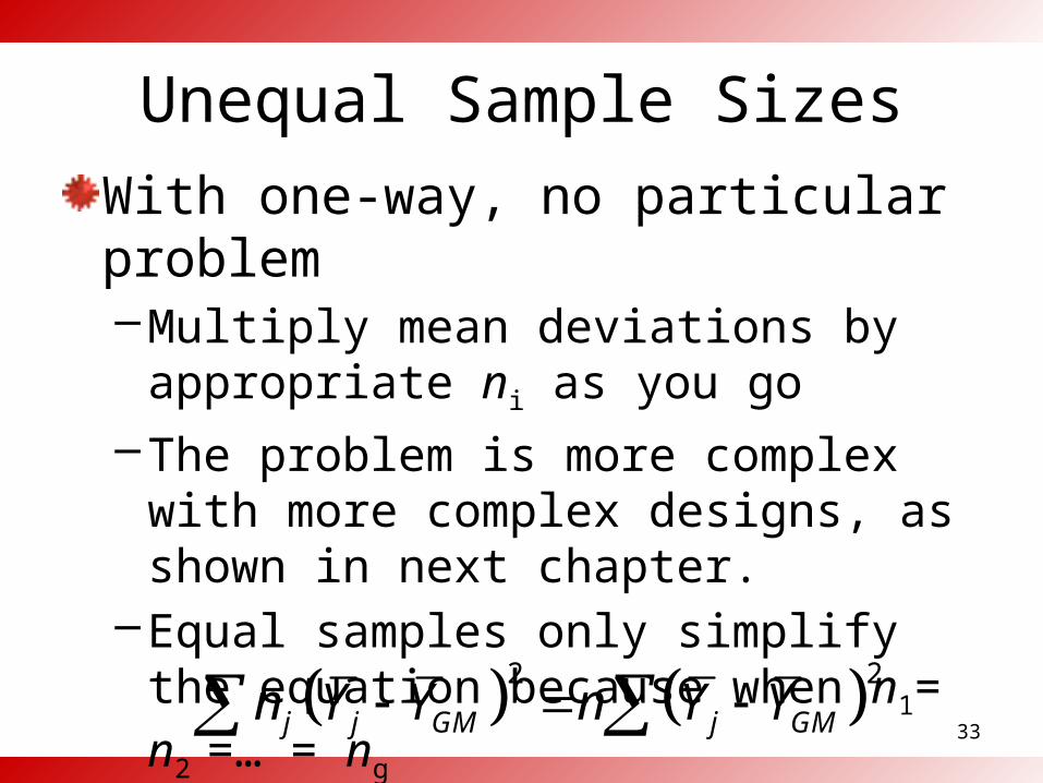
Unequal Sample Sizes
With one-way, no particular problem–Multiply mean deviations by appropriate
ni as you go
–The problem is more complex with more complex designs, as shown in next chapter.
–Equal samples only simplify the equation because when n1= n2 =… = ng
2 2
j j GM j GMn Y Y n Y Y
Psy 320 - Cal State Northridge
MULTIPLE COMPARISONS
34

Psy 320 - Cal State Northridge 35
Multiple Comparisons
Significant F only shows that not all groups are equal–We want to know what groups are
different.
Such procedures are designed to control familywise error rate.–Familywise error rate defined–Contrast with per comparison error rate
Psy 320 - Cal State Northridge 36
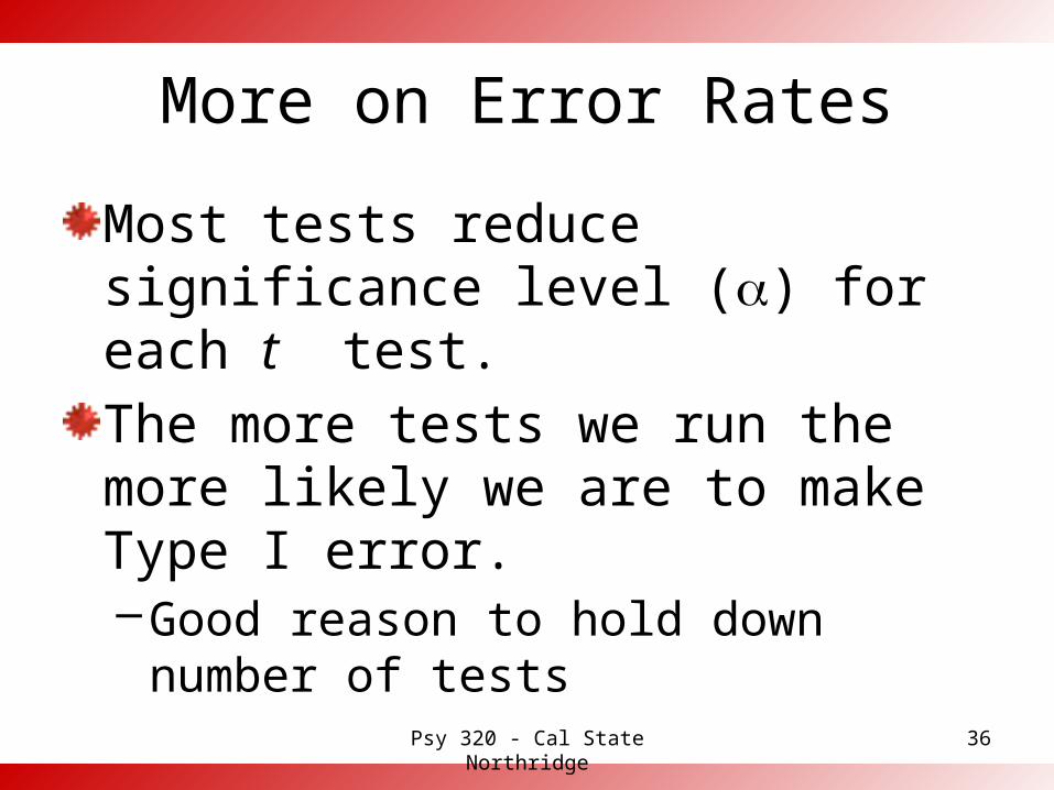
More on Error Rates
Most tests reduce significance level (a) for each t test.
The more tests we run the more likely we are to make Type I error.–Good reason to hold down number of
tests

Psy 320 - Cal State Northridge
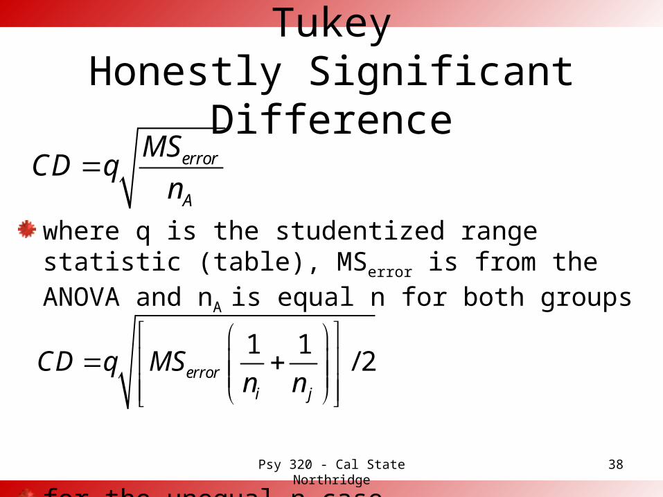
TukeyHonestly Significant DifferenceThe honestly significant difference (HSD) controls for all possible pairwise comparisons
The Critical Difference (CD) computed using the HSD approach
37
Psy 320 - Cal State Northridge
TukeyHonestly Significant Difference
where q is the studentized range statistic (table), MSerror is from the ANOVA and nA is equal n for both groups
for the unequal n case38
error
A
MSCD q
n
1 1/ 2error
i j
CD q MSn n

Psy 320 - Cal State Northridge
Tukey
Comparing Beechnut and Gerber–To compute the CD value we need to
first find the value for q–q depends on alpha, the total number of
groups and the DF for error.–We have 3 total groups, alpha = .05 and
the DF for error is 12–q = 3.77
39

Psy 320 - Cal State Northridge
TukeyWith a q of 3.77 just plug it in to the formula
This give us the minimum mean difference
The difference between gerber and beechnut is 3.8, the difference is significant 40
2.8673.77 2.86
5error
A
MSCD q
n
Psy 320 - Cal State Northridge 41
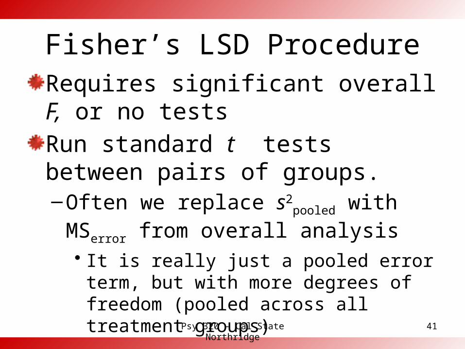
Fisher’s LSD ProcedureRequires significant overall F, or no tests
Run standard t tests between pairs of groups.–Often we replace s2
pooled with MSerror from overall analysis• It is really just a pooled error term, but with
more degrees of freedom (pooled across all treatment groups)
42
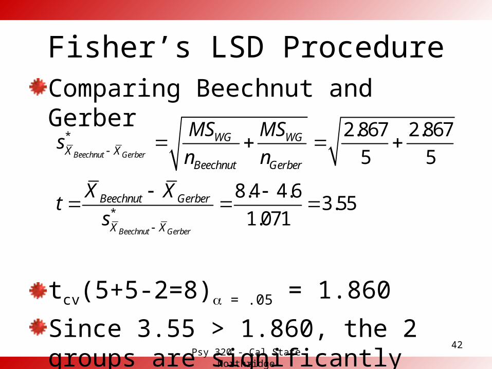
Fisher’s LSD ProcedureComparing Beechnut and Gerber
tcv(5+5-2=8) = .05 = 1.860
Since 3.55 > 1.860, the 2 groups are significantly different.
*
*
2.867 2.867
5 5
8.4 4.63.55
1.071
Beechnut Gerber
Beechnut Gerber
WG WGX X
Beechnut Gerber
Beechnut Gerber
X X
MS MSs
n n
X Xt
s
Psy 320 - Cal State Northridge

Psy 320 - Cal State Northridge 43
Bonferroni t TestRun t tests between pairs of groups, as usual–Hold down number of t tests–Reject if t exceeds critical value in
Bonferroni table
Works by using a more strict value of a for each comparison

Psy 320 - Cal State Northridge 44
Bonferroni tCritical value of a for each test set at .05/c, where c = number of tests run–Assuming familywise a = .05–e. g. with 3 tests, each t must be
significant at .05/3 = .0167 level.
With computer printout, just make sure calculated probability < .05/c

Psy 320 - Cal State Northridge 45
Assumptions for Analysis of Variance
Assume:–Observations normally distributed within
each population–Population variances are equal
• Homogeneity of variance or homoscedasticity
–Observations are independent

Psy 320 - Cal State Northridge
ASSUMPTIONS
46

Psy 320 - Cal State Northridge 47
Assumptions
Analysis of variance is generally robust to first two–A robust test is one that is not greatly
affected by violations of assumptions.

Psy 320 - Cal State Northridge
EFFECT SIZE
48
49
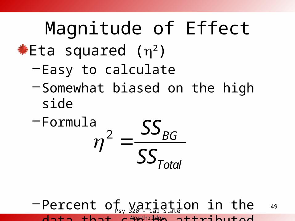
Magnitude of EffectEta squared (h2)–Easy to calculate–Somewhat biased on the high side–Formula
–Percent of variation in the data that can be attributed to treatment differences
2 BG
Total
SS
SS
Psy 320 - Cal State Northridge
50
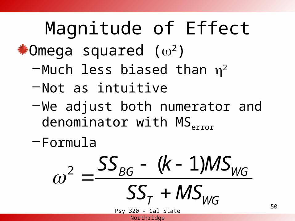
Magnitude of EffectOmega squared (w2)–Much less biased than h2
–Not as intuitive–We adjust both numerator and
denominator with MSerror
–Formula
2 ( 1)BG WG
T WG
SS k MS
SS MS
Psy 320 - Cal State Northridge

Psy 320 - Cal State Northridge 51
h2 = .52: 52% of variability in preference can be accounted for by brand of baby food
w2 = .42: This is a less biased estimate, and note that it is 20% smaller.
2
2
36.93.518
71.335
( 1) 36.93 2(2.867).420
71.335 2.867
BG
T
BG WG
T WG
SS
SS
SS k MS
SS MS
h2 and w2 for Baby Food

52
Other Measures of Effect SizeWe can use the same kinds of measures we talked about with t tests (e.g. d and d-hat)
Usually makes most sense to talk about 2 groups at a time or effect size between the largest and smallest groups, etc.
And there are methods for converting 2 to d and vice versa
Psy 320 - Cal State Northridge