| 209 | Henri Partanen | Modeling and measurement of ... · the ﬁeld of optical partial coherence...

Publications of the University of Eastern FinlandDissertations in Forestry and Natural Sciences No 209

Publications of the University of Eastern Finland

Dissertations in Forestry and Natural Sciences

isbn: 978-952-61-1534-4 (printed)

issn: 1798-5668

isbn: 978-952-61-1535-1 (pdf)

issn: 1798-5676

Henri Partanen

Modeling andmeasurement of partialspatial coherence

This thesis considers methods to

measure and model the coherence

function of the light sources. Young’s

interferometer realized with digital

micromirror devices is introduced

and the data is used to accurately

simulate the behavior of the beams.

Broad area laser diode is used as

an example of a clearly partially

coherent source with complicated

modal structure. Methods to modify

the coherence are considered.

Finally coupling of the partially

coherent beams into waveguides is

analyzed.

disser

tation

s | 209 | H

enr

i Pa

rta

nen

| Mo

delin

g an

d m

easu

remen

t of pa

rtial sp

atia

l coheren

ce

Henri PartanenModeling and

measurement of partialspatial coherence

HENRI PARTANEN

Modeling and

measurement of partial

spatial coherence



No 209

Academic Dissertation

To be presented by permission of the Faculty of Science and Forestry for public

examination in the Auditorium M101 in Metria Building at the University of

Eastern Finland, Joensuu, on December 18, 2015, at 12 o’clock noon.

Department of Physics and Mathematics

Grano Oy

Jyvaskyla, 2015

Editors: Prof. Pertti Pasanen, Prof. Kai Peiponen,

Prof. Pekka Kilpelainen, Prof. Matti Vornanen

Distribution:

University of Eastern Finland Library / Sales of publications

[email protected]

http://www.uef.fi/kirjasto

ISBN: 978-952-61-1534-4 (printed)

ISSNL: 1798-5668

ISSN: 1798-5668

ISBN: 978-952-61-1535-1 (pdf)

ISSNL: 1798-5668

ISSN: 1798-5676

Author’s address: University of Eastern Finland


P. O. Box 111

80101 JOENSUU

FINLAND

email: [email protected]

alt. email: [email protected]

Supervisors: Professor Jari Turunen, Dr.Tech.

University of Eastern Finland


P. O. Box 111

80101 JOENSUU

FINLAND


Associate Professor Jani Tervo, Ph.D.

University of Eastern Finland


P. O. Box 111

80101 JOENSUU

FINLAND


Reviewers: Professor Jose J. Gil, Ph.D.

Universidad de Zaragoza

Facultad de Educacion

San Juan Bosco 7

50009 ZARAGOZA

SPAIN


Associate Professor Juha Toivonen, Dr.Tech.

Tampere University of Techonology

Department of Physics

P. O. Box 692

33101 TAMPERE

FINLAND


Opponent: Associate Professor Sergei Popov, Dr.Tech.

Royal Institute of Technology (KTH)

Optics and Photonics Division

Electrum 229

164 40 KISTA

SWEDEN


ABSTRACT

This thesis contains studies on various aspects of partial spatial co-

herence of light. It includes purely theoretical considerations, nu-

merical simulations on partially coherent beam propagation, con-

struction and use of novel coherence measurement equipment, and

experimental results on characterization of light fields emitted by

real light sources. In the theoretical studies, the coupling of par-

tially coherent light into planar waveguides is investigated by means

of a coherent-mode decomposition of the incident field. Several

types of coherent-field representations are applied also to beams

radiated by broad-area laser diodes, which are used as practical

examples of spatially partially coherent light sources. Interferomet-

ric setups are constructed both for coherence measurement and for

the construction of interesting types of partially coherent beams of

light. The coherence functions of the considered light sources are

meandered by a novel realization of the classical Young’s double

pinhole experiment based on digital micromirror devises. The ac-

quired data is used to simulate the beam propagation with much

higher accuracy than before.

Universal Decimal Classification: 531.715, 535.3, 621.372.8, 621.375.826,

681.7.069.24

INSPEC Thesaurus: optics; light; light coherence; light propagation; sim-

ulation; modelling; optical variables measurement; light interferometry;

light interferometers; micromirrors; semiconductor lasers; optical planar

waveguides

Yleinen suomalainen asiasanasto: optiikka; valo; koherenssi; laserit; laser-

sateily; simulointi; mallintaminen; mittaus

Preface

I want to thank my supervisors Prof. Jari Turunen and Dr. Jani

Tervo for their great help and patience with me, without you this

work would not have been possible. You introduced me into the

world of coherence.

For financial support I am grateful to Tekniikan edistamissaatio

for a grant to finish the writing of this thesis. I am grateful to the

former and present heads of the Department of Physics and Math-

ematics Pasi Vahimaa, Markku Kuittinen, Seppo Honkanen and

Timo Jaaskelainen, for the opportunity to work in the university.

Thank you Pertti Paakkonen and Tommi Itkonen for helping me to

build and use my laboratory setups and other practical things.

During my studies I was able to work couple of months in Ger-

many, thank you Prof. Frank Wyrowski and Prof. Wolfgang Osten

for inviting me to these research visits to Jena and Stuttgart, and

for all the valuable knowledge shared over Europe. Also thank

you Olga Baladron Zorita, Christian Hellmann, Site Zhang, Daniel

Asoubar, Sandy Peterhansel, Christof Pruss, and all other who help-

ed and kept me company during these visits.

All the colleges and office roommates, thank you very much

Markus, Joonas, Najnin, Manisha, Subhajit, Rahul, Balu, Kimmo

and all others for good time in and outside of the university.

Thank you Sanna for being on my side during the good and bad

times. My deepest gratitude for my mother, you are the strongest

and most loving person I know, and my father, who did not see me

finish this work, you were the best dad in the world. This is for

you.

Joensuu December 2, 2015 Henri Partanen

LIST OF PUBLICATIONS

This thesis consists of the present review of the author’s work in

the field of optical partial coherence and the following selection of

the author’s publications:

I H. Partanen, J. Tervo, and J. Turunen, “Spatial coherence of

broad-area laser diodes,” Appl. Opt. 52, 3221–3228 (2013).

II H. Partanen, J. Turunen, and J. Tervo, “Coherence measure-

ment with digital micromirror device,” Opt. Lett. 39, 1034–

1037 (2014).

III H. Partanen, N. Sharmin, J. Tervo, and J. Turunen, “Specu-

lar and antispecular light beams,” Opt. Exp. 23, 28718–28727

(2015).

IV H. Partanen, J. Tervo, and J. Turunen, “Coupling of spatially

partially coherent beams into planar waveguides,” Opt. Exp.

23, 7879–7893 (2015).

Throughout the overview, these papers will be referred to by Ro-

man numerals.

AUTHOR’S CONTRIBUTION

The publications selected in this dissertation are original research

papers in the field of optical coherence theory. All papers are results

of group work. The author developed the ideas that lead to the

publications in collaboration with the co-authors. He has planned

and constructed the experimental setups used in all papers, carried

out nearly all of the experiments and numerical simulations, and

analyzed all the experimental results reported in the papers. He

has also participated actively in the writing of each manuscript.

LIST OF ABBREVIATIONS

The following abbreviations are used in this thesis:

ACF Angular correlation function

BALD Broad-area laser diode

CSD Cross spectral density function

DMD Digital micromirror device

GSM Gaussian Schell model

LED Light-emitting diode

VCSEL Vertical-cavity surface-emitting laser

WFI Wavefront folding interferometer

Contents

1 INTRODUCTION 1

2 PARTIAL SPATIAL COHERENCE 5

2.1 Cross-spectral density function . . . . . . . . . . . . . 5

2.2 Coherent-mode decomposition . . . . . . . . . . . . . 9

2.3 Schell-model sources . . . . . . . . . . . . . . . . . . . 10

2.4 Shifted elementary-field method . . . . . . . . . . . . 10

2.5 Summary . . . . . . . . . . . . . . . . . . . . . . . . . . 12

3 MODEL SOURCES AND FIELDS 13

3.1 Gaussian Schell model sources . . . . . . . . . . . . . 14

3.1.1 Coherent-mode representation . . . . . . . . . 16

3.1.2 Elementary-field representation . . . . . . . . 17

3.2 Cross-spectral density with finite number of modes . 17

3.3 Summary . . . . . . . . . . . . . . . . . . . . . . . . . . 20

4 REAL SOURCES: MODELING AND MEASUREMENT 21

4.1 Partially coherent light sources . . . . . . . . . . . . . 21

4.1.1 Broad area laser diodes . . . . . . . . . . . . . 21

4.1.2 Modes . . . . . . . . . . . . . . . . . . . . . . . 23

4.1.3 Coherence properties . . . . . . . . . . . . . . 24

4.2 Measurement systems . . . . . . . . . . . . . . . . . . 25

4.2.1 Imaging spectrometer . . . . . . . . . . . . . . 25

4.2.2 Young’s double pinhole system . . . . . . . . . 28

4.2.3 Interferometer realized with digital micromir-

ror device . . . . . . . . . . . . . . . . . . . . . 30

4.3 Gaussian Schell model beams generated by rotating

diffusers . . . . . . . . . . . . . . . . . . . . . . . . . . 31

4.4 Wavefront folding interferometer . . . . . . . . . . . . 33

4.5 Specular beams by wavefront folding interferometer 35

4.6 Summary . . . . . . . . . . . . . . . . . . . . . . . . . . 38

5 PROPAGATION AND COUPLING OF LIGHT 41

5.1 Analytical formulation . . . . . . . . . . . . . . . . . . 41

5.2 Numerical implementation . . . . . . . . . . . . . . . 42

5.2.1 Propagation of broad area laser diode beam . 43

5.3 Coupling into planar waveguides . . . . . . . . . . . . 46

5.4 Summary . . . . . . . . . . . . . . . . . . . . . . . . . . 51

6 DISCUSSION AND CONCLUSIONS 53

REFERENCES 57

1 Introduction

Light emitted by natural sources, such as the sun and other stars,

forest fires, or fluorescent creatures lurking in deep oceans, is nearly

spatially incoherent. In simple terms, this means that if we apply

a two-pinhole mask to isolate two small spatially separated areas

of the field emitted by the source and let the radiation from the

pinholes propagate further, the observed intensity distribution is

essentially the sum of the intensity distributions seen when only

one of the pinholes is open. Several man-made light sources, such

as lasers, exhibit rather different behavior: if we again sample the

field at two spatially separated points and let the resulting fields

overlap, interference fringes of high contrast are observed. In this

case the field radiated by the source can be characterized as being

highly spatially coherent. However, there are many light sources

with spatial coherence properties between these two extremes. Such

partially spatially coherent light sources produce fringes with re-

duced contrast in the two-pinhole experiment.

Optical coherence theory provides the methodology to deal with

all kinds of light sources referred to above [1–3]. In particular, it al-

lows one to define quantitatively concepts such as the degree of

spatial coherence, which specifies how well light fields emanating

from the two pinholes can interfere. This theory is of central impor-

tance in optics since the effects of the state of spatial coherence of

light extend far beyond the two-pinhole experiment. With spatially

coherent laser light we can easily see many kinds of interference

patterns, including speckle patterns, even when we try to use laser

light for even illumination [4, 5]. On the other hand, with thermal

light, it is very difficult to see any kind of interference unless the

pinholes are spaced within a wavelength-scale distance apart. In

the absence of coherent light sources, proving the wave nature of

the light was difficult two hundred years ago [6–8]. The visibility

of the interference fringes is indeed the traditional definition for

Dissertations in Forestry and Natural Sciences No 209 1

Henri Partanen: Modeling and measurement of partial spatial coherence

the degree of spatial coherence of light [9], and will be used in this

thesis as the basis of our measurement setups.

The degree of coherence is not just a single number, but it de-

pends on the measurement coordinates (pinhole positions). Nor-

mally, when the measurement points get further away from the

each other, the degree of coherence decreases. On the other hand,

when the points approach each other, the degree of coherence goes

to unity. However, such qualitative considerations are not sufficient

to describe most partially coherent sources, since spatial coherence

generally depends also on the absolute positions of the pinholes.

To fully model partially coherent light it is, first of all, necessary

to quantify the concept of partial coherence, to which end opti-

cal coherence theory provides the means. Generally, in this the-

ory, partially coherent fields are described by correlation functions

that characterize the nature of partially coherent light in statistical

terms. Such correlation function depend, in addition to the spatial

coordinates, also on frequency or time. Further, to be exact, the

state of polarization of the vectorial light field must be taken into

account.

Partial spatial coherence of light implies major numerical mod-

eling problems. The propagation of fully coherent light emitted by

a planar source can be treated by two-dimensional integrals, but

for partially coherent light the corresponding propagation integrals

become four-dimensional. Likewise, the measurement of the op-

tical properties of partially coherent light is a hugely more com-

plicated task than the characterization of a fully spatially coherent

field. Treating these problems is the central theme of the present

thesis. On the theoretical side, the backbone of the work is the

representation of partially coherent light as superpositions of fully

coherent modal subfields. The demanding task is to find them.

The modes may, for example, correspond to resonator modes of the

laser, and we may simulate them, if we know the resonator proper-

ties. However, real sources often have imperfections and the shape

of the modes may differ considerably from predictions of simple

models. Therefore we may have to measure the coherence function

2 Dissertations in Forestry and Natural Sciences No 209

Introduction

and solve the modes from it. In this thesis we introduce some mea-

surement systems to do this, and discuss how light can be modeled

efficiently.

This thesis is organized as follows. In Chapter 2 we introduce

the basic concepts of partial spatial coherence. In Chapter 3 we

introduce the Gaussian Schell-model source as a simple example of

spatially partially coherent sources, and describe how such a source

can be modeled numerically using different modal methods. In

Chapter 4 we consider real non-ideal light sources and methods to

measure their coherence properties, concentrating in particular on

broad-area laser diodes. In Chapter 5 we discuss analytical and

numerical methods to propagate light in free space and to couple

light fields into planar waveguides. Finally, in Chapter 6, some

conclusions are drawn and certain possible future directions of the

research are outlined.


2 Partial spatial coherence

In this Chapter we define the basic concepts needed to describe

the spatial coherence properties of light. We begin by defining the

fundamental correlation function of stationary fields in the space-

frequency domain, namely the cross spectral density function (CSD),

which describes field correlations between two spatial position at a

given frequency. Then representations of the CSD by means of su-

perpositions of fully coherent modes are described.

2.1 CROSS-SPECTRAL DENSITY FUNCTION

Restricting the discussion to scalar theory of light, we consider a

single component E(r, t) of the electric field at position r = (ρ, z) =

(x, y, z) and time t. In many circumstances it is more convenient to

consider the field in the frequency domain. To this end we will use

the complex analytic signal representation [1]

E(r, t) =∫ ∞

0E(r, ω) exp (−iωt) dω, (2.1)

where

E(r, ω) =1

2π

∫ ∞

−∞E(r, t) exp (iωt) dt (2.2)

is the electric field at position r and frequency ω. For partially

coherent light the electric field fluctuates more or less randomly

between two spatial coordinates and two frequencies or instants of

time. A statistical description of the field is then appropriate and we

may define its correlation properties in the space-frequency domain

by introducing a two-frequency CSD

W(r1, r2, ω1, ω2) = �E∗(r1, ω1)E(r2, ω2)� (2.3)

where the sharp brackets denote an ensemble average

�E∗(r1, ω1)E(r2, ω2)� = limn=∞

1

N

N

∑n=1

E∗n(r1, ω1)En(r2, ω2) (2.4)



over a set of individual field realizations En(r, ω), which may be e.g.

individual pulses in pulse trains generated by mode-locked lasers

or supercontinuum sources.

Let us assume that the light field is stationary, i.e., its space-

time correlation properties do not depend on the origin of time but

only on the time difference t2 − t1. In this case different spectral

components of the field become mutually uncorrelated [1] and the

the two-frequency CSD takes the form

W(r1, r2, ω1, ω2) = W(r1, r2, ω1)δ(ω1 − ω2), (2.5)

where the CSD describing a stationary field,

W(r1, r2, ω) = �E∗(r1, ω)E(r2, ω)�, (2.6)

depends spectrally only on a single (absolute) frequency ω. Now

the spectral density (intensity of the field at position r and fre-

quency ω) is defined as

S(r, ω) = W(r, r, ω) = �|E(r, ω)|2�. (2.7)

Furthermore, we may also introduce a normalized form of the CSD,

µ(r1, r2, ω) =W(r1, r2, ω)

[S(r1, ω)S(r2, ω)]1/2, (2.8)

known as the complex degree of spectral coherence. This complex-

valued function satisfies the inequalities |µ(r1, r2, ω)| ≤ 1, where

the upper bound means complete spatial coherence and the lower

bound indicates full incoherence of the field at frequency ω.

In this thesis we will deal mainly with quasimonochromatic

fields, which have a narrow spectral bandwidth ∆ω around a given

center frequency ω0 of the spectrum. In this case the dependence

of the CSD on ω is typically insignificant and we therefore leave it

implicit from now on for brevity of notation.

All genuine cross-spectral functions have to be nonnegative def-

inite kernels, which means they have to obey (at any transverse

plane z = constant) the condition [10, 11]

Q( f ) =∫∫ ∞

−∞W(ρ1, ρ2) f ∗(ρ1) f (ρ2)d2ρ1 d2ρ2 ≥ 0, (2.9)


Partial spatial coherence

for any choice of the function f (ρ). Also, for all CSD functions, the

following inequality holds:

|W(ρ1, ρ2)|2 ≤ W(ρ1, ρ1)W(ρ2, ρ2) = S(ρ1)S(ρ2). (2.10)

Violating these conditions may lead to clearly non-physical results,

such as negative intensities in some positions. Later we see how

measurement errors may lead to such a situation. The CSD is also

Hermitian, i.e.,

W(r1, r2) = W∗(r2, r1). (2.11)

This, for example, means it is enough to measure only one half

of the matrix of a sampled CSD data array. A useful criterion to

recognize a genuine CSD is that all of them can be expressed in the

form

W(ρ1, ρ2) =∫ ∞

∞p(v)H∗(ρ1, v)H(ρ2, v)d2v, (2.12)

where H(ρ, v) is an arbitrary kernel and p(v) is a non-negative

function [10, 11].

Strictly speaking, in the case of narrow-band fields such as those

emitted by multimode lasers, we do not usually measure the CSD

since frequency-resolved measurements are difficult. Instead, we

measure its frequency-integrated form

J(ρ1, ρ2) =∫ ∞

0W(ρ1, ρ2, ω)dω, (2.13)

known as the mutual intensity. In Papers I and II we indeed used

mutual intensity J(ρ1, ρ2) as the measure of spatial coherence. Nev-

ertheless, in this thesis we call all measured coherence functions

CSD for consistency, as all light sources we are studying are at

least quasimonochromatic. Also, when calculating the propagation

of different field modes, which (unless degenerate) are centered at

different frequencies, we should in principle treat every individual

wavelength individually to be exact. However, the error made by

using only the central wavelength is negligible.



Let us now introduce an angular form of the CSD, known as the

angular cross-correlation function (ACF), defined as

A(κ1, κ2) =∫∫ ∞

−∞W(ρ1, ρ2) exp [−i(κ1 · ρ1 − κ2 · ρ2)] d2ρ1 d2ρ2,

(2.14)

where κ =(

kx, ky

)

is the transverse componet of the wave vector

k =(

kx, ky, kz

)

. We may now define the angular spectral density as

F(κ) = A(κ, κ) (2.15)

and the complex degree of angular coherence

µ(κ1, κ2) =A(κ1, κ2)

[F(κ1, ω)F(κ2)]1/2

(2.16)

in analogy with their counterparts in the spatial domain. In the far

zone the CSD is then [1]

W∞(r1s1, r2s2) = (2πk)2 cos θ1 cos θ2 A(σ1, σ2)exp[ik(r1 − r2)]

r1r2,

(2.17)

where r = |r|, s = r/r is the unit position vector, σ =(

sx, sy

)

=

(x/r, y/r) is its transverse component, θ is the angle between s and

the z axis, and k = 2π/λ is the wave number. The function

J(rs) = r2W∞(rs, rs) = (2πk)2 cos2 θF(σ), (2.18)

known as the radiant intensity, describes the angular distribution

of optical intensity in the far zone.

The theory presented above for scalar fields can be expanded

to vectorial electromagnetic fields [12], which leads to the concept

of a cross-spectral tensor and allows one to study the combined ef-

fects of partial coherence and partial polarization. In this thesis we

consider only linearly polarized light fields, which are reasonably

directional. In such circumstances the scalar approach, in which

only one field component is considered, is a good model.



2.2 COHERENT-MODE DECOMPOSITION

When propagation problems with two-dimensional fields are con-

sidered, dealing with the CSD directly usually leads to numerically

untractable problems; Eqs. (2.14)–(2.18) show that four-dimensional

integrals need to be evaluated. Luckily, any CSD may be repre-

sented as an incoherent sum of coherent modes, which reduces the

propagation formulas in sums of two-dimensional integrals. Specif-

ically, we may write the field across the source plane in the form of

a Mercer-type coherent-mode expansion [13]

W(ρ1, ρ2) = ∑m

cmv∗m(ρ1)vm(ρ2), (2.19)

where cm are real and nonnegative weight factors and vm(ρ) are

the modal wave functions. If the CSD is known, these weights and

mode functions can be found evaluating the eiqenvalues and eiqen-

functions of the Fredholm integral equation

∫ ∞

−∞W(ρ1, ρ2)vm(ρ1)d

2ρ1 = cmvm(ρ2). (2.20)

Once the eigenvalues and eigenmodes are known for the field at

the source plane, the propagated CSD

W(r1, r2) = ∑m

cmv∗m(r1)vm(r2) (2.21)

can be evaluated using the standard two-dimensional propagation

integrals for fully coherent light to relate the modal contributions

vm(r) to vm(ρ).

Considering y-invariant fields, the numerical solution of the

eigenvalues and modes from Eq. (2.20) involves discretizing the

CSD W(x1, x2) and solving the matrix equation

W = VIV−1, (2.22)

where W contains the CSD data, the columns of V are the eigen-

modes, I is a diagonal matrix with corresponding eigenvalues, and

all three are N × N square matrices if N modes are retained in



Eq. (2.20). This equation can be solved using standard numerical

libraries found in many software packages such as Matlab [14]. For

two-dimensional sources with four-dimensional CSDs W(ρ1, ρ2) the

task becomes more demanding, and might require custom numer-

ical functions. Fortunately, in some important special cases the

modes and their weights are known analytically.

2.3 SCHELL-MODEL SOURCES

Many light sources obey the Schell model, where the complex de-

gree of spatial coherence does not depend on absolute positions ρ1

and ρ2, but only on their difference ∆ρ = ρ2 − ρ1. In this case the

CSD has the form [15]

W(ρ1, ρ2) = [S(ρ1)S(ρ2)]1/2

µ(∆ρ). (2.23)

This is convenient for coherence measurements since one would not

have to measure all coherence between all combinations of the co-

ordinates, which for a two-dimensional planar source would mean

a four-dimensional matrix. Instead, it is enough to vary just the

separation between the measurement points.

It is also possible to define sources that are of the Schell-model

form in the space-frequency domain. In this case we write the ACF

in a form analogous to Eq. (2.23), i.e.,

A(κ1, κ2) = [F(κ1)F(κ2)]1/2

γ(∆κ), (2.24)

where ∆κ = κ2 − κ1. Hence the complex degree of angular coher-

ence, γ(∆κ), now depends only on the difference between the two

spatial-frequency vectors.

2.4 SHIFTED ELEMENTARY-FIELD METHOD

While the coherent-mode representation can model any arbitrary

field, finding the coherent modes is usually a very demanding task,

with only a few analytical solutions being known. We therefore

proceed to describe another method, which deals with a specific



class of genuine CSDs but is nevertheless applicable to wide variety

of cases (if not exactly, at least to a good approximation).

In late 1970s Gori and Palma introduced a method to model

Gaussian Schell-model sources [16, 17] using a set of laterally or

angularly shifted ‘elementary’ modes, which can be summed in-

coherently to form the correct CSD. This model was later extended

to more general planar sources [18], three-dimensional sources [19],

partially temporally coherent pulse trains [20], and vectorial electro-

magnetic sources [21]. A review of this elementary-mode method

can be found in [22]. The elementary-field method has been ap-

plied, e.g., to analyzed excitation of surface plasmons under par-

tially coherent illumination [23], beam shaping problems with vari-

ous types of illumination and shaping elements [24,25], and optical

imaging problems [26].

Considering the formulation of the elementary-field method in

the spatial domain, we assume that the CSD at the source plane can

be represented as

W(ρ1, ρ2) =∫ ∞

−∞p(ρ′) f ∗(ρ1 − ρ

′) f (ρ2 − ρ′)d2ρ′, (2.25)

which implies that its spectral density is given by

S(ρ) =∫ ∞

−∞p(ρ′)| f (ρ − ρ

′)|2 dρ′. (2.26)

Here f (ρ) is a well-behaved function called the elementary field

mode and p(ρ′) a non-negative weight function. This means that

the field is expressed as sum of identical but spatially shifted and

weighted modes. Clearly, Eq. (2.25) represent a genuine CSD since

it is a special case of Eq. (2.12): now p(ρ′) takes the role of p(v) and

f (ρ − ρ′) that of H(ρ, v).

It is a simple matter to show, using Eq. (2.14), that if the source-

plane field is of the form of Eq. (2.25), the angular cross-correlation

function obeys the Schell model (2.24) provided that

f (ρ) =1

(2π)2

∫ ∞

−∞[F(κ)]1/2 exp(iρ · κ)d2κ (2.27)



and

p(ρ′) =1

(2π)2

∫ ∞

−∞γ(∆κ) exp(iρ′ · ∆κ)d2

∆κ. (2.28)

In view of Eq. (2.27), the elementary field can be determined di-

rectly from the angular spectral density, which is an easily measur-

able quantity. The determination of the weight function generally

requires spatial coherence measurements in the far zone, which

may in practice be a difficult task. This task is, however, greatly

simplified if the source is known to be quasihomogeneous, i.e., its

spatial coherence area is small compared to the source size. In this

case one may use the source-plane intensity profile directly as the

weight function since S(ρ) ≈ p(ρ) [18].

2.5 SUMMARY

The cross-spectral density function (CSD) is a nonnegative definite

function that fully defines the spatial coherence properties of spa-

tially partially coherent light. Even though the CSD is an important

mathematical concept, its direct numerical handling in, e.g., prop-

agation problems is often too difficult. Therefore it is useful to

represent the CSD in terms of sums of coherent modes introduced

in this Chapter. The Mercer-type coherent-mode decomposition is

fully accurate, but its determination can in many cases be a rather

heavy task. On the other hand, the elementary-field representation

is numerically highly efficient whenever it is applicable.


3 Model sources and fields

In this Chapter we introduce a useful idealized model for spa-

tially partially coherent light sources, known as the Gaussian Schell

model (GSM) [15]. This model is capable of describing several

real partially coherent sources and beams generated by them in an

approximate way, including excimer [27] and free-electron [28, 29]

lasers beams and, as we will see in Chapter 4, also widely diverg-

ing fields emanating from broad-area laser diodes (Papers I and II).

Both coherent-mode and elementary-field representation are shown

to be applicable to GSM sources. The propagation of fields gener-

ated by GSM sources can be governed analytically [30], but we also

consider numerical modeling of their propagations. This will allow

us to assess the accuracy of finite or discrete modal representations,

providing useful yardsticks for numerical modeling light propaga-

tion from more complicated realistic sources including broad-area

laser diodes to be considered later on in this thesis.

In the case of GSM sources, the coherent modes have a math-

ematical form of Hermite–Gaussian modes generated in spherical-

mirror resonators [31, 32], with a specific set of modal weights [33,

34]. Other model sources that do not generally obey the Schell

model can be constructed using different sets of modal weights:

multi-spatial-mode lasers in either gas, solid-state, or semiconduc-

tor form can all emit such spatially partially coherent radiation. On

the other hand, GSM sources have an elementary-field expansion,

which involves a Gaussian elementary field with a Gaussian weight

distribution. Retaining the assumption that the elementary field is

still Gaussian but letting the weight profile be more arbitrary again

leads to useful generalizations with spatial profiles and spatial co-

herence functions that are not Gaussian form. In Chapter 4 such

a model will be applied to multimode broad-area edge-emitting

semiconductor lasers.



3.1 GAUSSIAN SCHELL MODEL SOURCES

The most widely used model source in the theory of spatially par-

tially coherent optics is undoubtedly the GSM source, which gener-

ates GSM fields that may exhibit widely different divergence prop-

erties depending on the chosen combination of the source param-

eters. In this model both the spectral density and the degree of

spatial coherence at the source plane have Gaussian shapes. The

most prominent features of the GSM beams are that their shape

stays constant as they propagate. Their propagation behavior can

be determined analytically using the same kind of propagation pa-

rameters that are employed to describe the fully coherent Gaussian

beams, as shown explicitly in Ref. [30]. Indeed, GSM beams can be

seen as natural generalizations of traditional Gaussian beams into

the domain of spatially partially coherent optics.

In what follows, we first describe the properties of a GSM source

(or the waist of a GSM beam). Since the CSD of a GSM beam is sep-

arable in transverse coordinates, we only consider its representation

in the x-direction, with the understanding that a strictly similar de-

scription is valid in the y-direction as well. In the case of anisotropic

GSM beams [35, 36], the parameters that define the source size and

its coherence area are generally different in x and y directions.

Consider the general representation of a Shell-mode source de-

scribed by Eq. (2.23). When written in a y-invariant form, this ex-

pression reads as

W(x1, x2) = [S(x1)S(x2)]1/2

µ(∆x). (3.1)

The GSM source is described by Gaussian distributions of the spec-

tral density and degree of spatial coherence: we may write

S(x) = S0 exp

(

−2x2

w20

)

(3.2)

and

µ(∆x) = exp

(

−∆x2

2σ20

)

, (3.3)


Model sources and fields

where w0 and σ0 are the characteristic widths of the intensity pro-

file and degree of spatial coherence, respectively. Figure 3.1 illus-

trates the full CSD and the complex degree of coherence (in this

case real-valued) of a one-dimensional GSM source when plotted

as a function of the absolute coordinates x1 and x2.

(a) |W (x1, x2)|

x2/λ

x1/λ−500 0 500

−500

0

500(b) |µ(x1, x2)|

x2/λ

x1/λ−500 0 500

−500

0

500

Figure 3.1: Coherence properties of a Gaussian Schell-model source. The cross-spectral

density function (left) and the complex degree of spatial coherence (right) when w0 = 300λ

and σ0 = 80λ.

When a beam radiated by a GSM source propagates in free

space, its intensity distribution remains Gaussian, but the trans-

verse scale expands according to the law

w(z) = w0

[

1 + (z/zR)2]1/2

, (3.4)

where

zR =πw2

0

λβ (3.5)

and

β =[

1 + (w0/σ0)2]−1/2

. (3.6)

The absolute value of the complex degree of coherence also remains

Gaussian, but the width σ0 at the source plane is replaced with σ(z).

An important feature of GSM beams is that ratio of the beam width



and coherence width stays constant as the beam propagates, i.e.,

α =σ0

w0=

σ(z)

w(z)(3.7)

is a propagation-invariant quantity. While being real-valued at the

source plane, the complex degree of coherence acquires a quadratic

phase as the beam propagates [30]. In Chapter 5.3 we will introduce

some extensions to this basic Gaussian Schell-model beam.

3.1.1 Coherent-mode representation

Even though the free-space propagation of the GSM beam can be

governed analytically, the situation is different if the beam is dis-

turbed by any object such as a simple aperture. The propagation of

such a disturbed beam must be evaluated numerically and then it is

convenient to represent the source in terms of its coherent modes.

The coherent-mode expansion of the GSM source is

W(x1, x2) =∞

∑m=0

cmv∗m(x1)vm(x2). (3.8)

The eigenfunctions are of Hermite–Gaussian form [33, 34]

vm(x) =

(

2

πw20β

)1/4 1

(2mm!)1/2Hm

( √2x

w0

√

β

)

exp

(

− x2

w20β

)

,

(3.9)

where Hm(x) is a Hermite polynomial of order m, and the eigen-

values (or weights of the modes) are

cm = S0

√2πw0

β

1 + β

(

1 − β

1 + β

)m

. (3.10)

When the beam propagates in free space, the eigenmodes expand

laterally and acquire a quadratic phase in precisely the same way

as the modes emanating from a spherical-mirror resonator.



3.1.2 Elementary-field representation

An alternative way to model GSM sources is the shifted elementary

mode method. Now the CSD function is expressed in the form

analogous to Eq. (2.25), as

W(x1, x2) =∫ ∞

−∞p(x′) f ∗(x1 − x′) f (x2 − x′)dx′. (3.11)

The elementary modes f (x) and their weight function p(x′) both

have Gaussian shapes

f (x) = f0 exp

(

− x2

w2e

)

(3.12)

and

p(x′) = p0 exp

(

−2x′2

w2p

)

. (3.13)

Their widths depend on the original beam and coherence widths of

the beam according to [22, 37].

wp = w0

√

1 − β2 (3.14)

and

we = w0β. (3.15)

The elementary field, of course, propagates in free space according

to the usual propagation laws for fully coherent Gaussian beams.

3.2 CROSS-SPECTRAL DENSITY WITH FINITE NUMBER OF

MODES

In numerical modeling one must truncate the coherent-mode repre-

sentation of the GSM source by including only modes up to m = M

in Eq. (3.8), with M chosen large enough to represent the field with

a sufficient accuracy; the effective number of modes of a partially

coherent field is analyzed in Ref. [38]. The results with a finite num-

ber of modes are illustrated in Fig. 3.2, where the properties of the



GSM source are analyzed using five lowest-order coherent modes

and assuming the same parameters as in Fig. 3.1. The inclusion of

five modes is quite sufficient to represent the intensity distribution

S(x) well, as seen from Fig. 3.2(c). Also the CSD plot in Fig. 3.2(a)

is nearly identical to the ideal result shown in Fig. 3.1(a). When

the complex degree of coherence is considered, clear differences

between the finite approximation in Fig. 3.2(b) and the exact result

shown in Fig. 3.1(b) are seen. However, these are significant only in

regions where the beam intensity is low.

(a) |W (x1, x2)|

x2/λ

x1/λ−500 0 500

−500

0

500(b) |µ(x1, x2)|

x2/λ

x1/λ−500 0 500

−500

0

500

−500 0 500

−0.5

0

0.5

1

(c)

S(x),v m

(x)

x/λ

Figure 3.2: Representation of a GSM source with a finite number of coherent modes.

(a) Cross-spectral density function. (b) Complex degree of spatial coherence. (c) Field

profiles of some lowest-order eigenmodes (thin black, red, blue and cyan lines), the intensity

profile S(x) with five modes included (thick solid line), and the exact Gaussian intensity

profile (dashed line).

The number of modes that need to be included in the coherent-

mode representation depends on the degree of coherence of the

source, characterized by the parameter β. In view of Eq. (3.10), we



havecm

c0=

(

1 − β

1 + β

)m

(3.16)

Therefore, denoting by M the index of the highest-order coherent

mode included in the numerical analysis, we have cM/c0 < R if

M >log R

log [(1 − β)/(1 + β)]. (3.17)

We have found that the choice R = 0.05 is sufficient to ensure nu-

merical convergence. Hence the required value of M can be deter-

mined from Eq. (3.17) for a GSM source of any state of coherence.

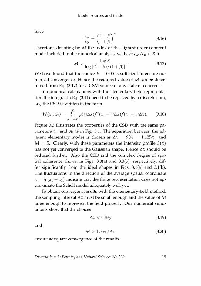
In numerical calculations with the elementary-field representa-

tion the integral in Eq. (3.11) need to be replaced by a discrete sum,

i.e., the CSD is written in the form

W(x1, x2) =M

∑m=−M

p(m∆x) f ∗(x1 − m∆x) f (x2 − m∆x). (3.18)

Figure 3.3 illustrates the properties of the CSD with the same pa-

rameters w0 and σ0 as in Fig. 3.1. The separation between the ad-

jacent elementary modes is chosen as ∆x = 90λ = 1.125σ0, and

M = 5. Clearly, with these parameters the intensity profile S(x)

has not yet converged to the Gaussian shape. Hence ∆x should be

reduced further. Also the CSD and the complex degree of spa-

tial coherence shown in Figs. 3.3(a) and 3.3(b), respectively, dif-

fer significantly from the ideal shapes in Figs. 3.1(a) and 3.1(b).

The fluctuations in the direction of the average spatial coordinate

x = 12 (x1 + x2) indicate that the finite representation does not ap-

proximate the Schell model adequately well yet.

To obtain convergent results with the elementary-field method,

the sampling interval ∆x must be small enough and the value of M

large enough to represent the field properly. Our numerical simu-

lations show that the choices

∆x < 0.8σ0 (3.19)

and

M > 1.5w0/∆x (3.20)

ensure adequate convergence of the results.



(a) |W (x1, x2)|

x2/λ

x1/λ−500 0 500

−500

0

500(b) |µ(x1, x2)|

x2/λ

x1/λ−500 0 500

−500

0

500

−500 0 5000

0.5

1(c)

S(x),|f

m(x)|2

x/λ

Figure 3.3: Representation of a GSM source with a finite number of shifted elementary

modes. (a) Cross-spectral density function. (b) Complex degree of spatial coherence.

(c) Field profiles of some elementary modes (thin lines), the intensity profile S(x) with

11 elementary modes included (thick solid line), and the exact Gaussian intensity profile

(dashed line).

3.3 SUMMARY

In this Chapter the Gaussian Schell model was presented as a useful

tool for approximate description of many real spatially partially co-

herent sources. Also the coherent-mode and elementary-field rep-

resentations of GSM sources were introduced. In addition, the ef-

fects of including only a finite number of modes were illustrated

numerically.


4 Real sources: modeling and

measurement

In the previous Chapter we discussed ideal source models, whereas

in this Chapter we will introduce certain real-life partially coherent

light sources. Methods for characterization of their spatial coher-

ence properties are discussed and experimental results are given.

4.1 PARTIALLY COHERENT LIGHT SOURCES

To be exact, there are no light source that are spatially fully co-

herent or completely incoherent, though single-mode lasers can be

considered as fully coherent sources for all practical purposes and

thermal sources as well as surface-emitting light-emitting diodes

(LEDs) have spatial coherence areas with dimensions in the scale

of the wavelength. There are several important laser sources with

partial spatial coherence properties, including excimer lasers [27],

free-electron lasers [28,29,39], many vertical-cavity surface-emitting

laser (VCSEL) arrays [40–43], and random lasers [44,45]; see Ref. [37]

for a more thorough discussion. Also multimode edge-emitting

semiconductor lasers are spatially partially coherent, and they will

be considered in more detail below.

4.1.1 Broad area laser diodes

The class of partially coherent light sources we concentrate on are

Broad Area Laser Diodes (BALDs), which are high-power edge-

emitting semiconductor light sources [46–50]. Figure 4.1 sketches

the shape of the resonator and the asymmetric spreading of the

BALD beam. We denote the resonator dimensions by Lx, Ly, and

Lz. The main difference between BALDs and typical laser diodes

used in, e.g., telecommunication applications is the much wider



resonator cavity of BALDs. Typically Lx ∼ 100 µm, which allows a

large number of lateral modes to be excited and therefore facilitates

high output power. However, as the modes are mutually uncor-

related, this also leads to a low degree of spatial coherence and

reduced beam quality [51, 52]. In y direction the resonator is much

narrower (Ly ∼ 1 µm), which allows only one mode, and hence the

light in y direction is essentially spatially coherent. In modeling the

spatial coherence of BALDs, we can therefore restrict our study to

x direction alone.

Figure 4.1: The BALD resonator and the type of beam radiated by it.

Strictly speaking, there are nanosecond-scale temporal fluctua-

tions in the temporal intensity of BALD emission in continuous-

wave operation [53–55]. Nevertheless, we can treat BALDs as sta-

tionary sources, though their temporal coherence is low because

of the large number of co-existing and mutually uncorrelated lon-

gitudinal modes. We will see direct evidence of the longitudinal

(as well as transverse) mode structure when studying a particular

BALD experimentally in Sect. 4.2.1.

Figure 4.2 shows how the measured optical power increases lin-

early with driving current above the lasing threshold (at ∼ 600 mA).

Below this threshold the BALD acts essentially as an edge-emitting

LED and emits almost spatially incoherent light in x direction (while

the emission remains highly coherent in y direction). When the

driving current rises in the linear (lasing) region, more and more


Real sources: modeling and measurement

transverse modes are excited and the coherence properties of the

BALD change (Paper II).

200 400 600 800 1000 1200 1400 1600 18000

0.2

0.4

0.6

0.8

current [mA]

pow

er[W

]

200 400 600 800 1000 1200 1400 1600 180010

−4

10−3

10−2

10−1

100

current [mA]

pow

er[W

]

Figure 4.2: BALD power as function of the driving current in (a) linear scale and (b) in

logarithmic scale.

4.1.2 Modes

In the ideal case the BALD resonator may be modeled as a planar

waveguide with well-defined modes. Now, as Lx ≫ λ, the tails

of the modal fields outside the resonator in the x direction are in-

significant, and it is enough to model the field inside the resonator

as a sinusoidal wave. In other words, we treat the dielectric wave-

guide as a mirror waveguide with perfectly conducting mirrors at

the edges x = ±Lx/2. This approximation is much closer to be-

ing realistic than the use of Hermite–Gaussian modes, which may

be used to approximate the exact waveguide modes in the case of

narrower multimode resonators. In reality the resonator has imper-

fections and the shape of the modes is rather irregular, especially



with the BALD specimen we studied. Nevertheless, it is useful to

model the modes at the source plane by writing

vm(x) =

√2/Lx sin(πmx/Lx) if |x| ≤ Lx/2 and m is even

√2/Lx cos(πmx/Lx) if |x| ≤ Lx/2 and m is odd

0 otherwise,

(4.1)

where m = 1, 2, 3, . . . is the mode index. The modal fields in the far

zone can be determined by calculating the Fourier transforms

am(kx) =1

2π

� ∞

−∞vm(x) exp (−ikx x) dx. (4.2)

This gives

am(kx) =

im(−1)m/2√

2Lxsin(kx Lx/2)

π2m2 − k2x L2

x

if m is even

m(−1)(m−1)/2√

2Lxcos(kxLx/2)

π2m2 − k2x L2

x

if m is odd(4.3)

and by plotting these we see that in the far field a single mode

forms two symmetric peaks.

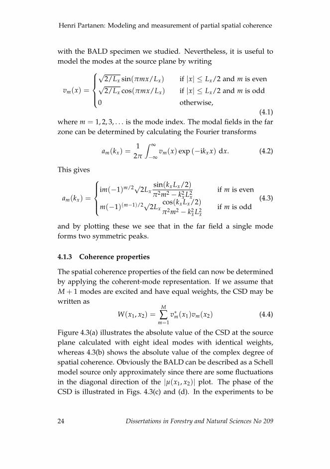
4.1.3 Coherence properties

The spatial coherence properties of the field can now be determined

by applying the coherent-mode representation. If we assume that

M + 1 modes are excited and have equal weights, the CSD may be

written as

W(x1, x2) =M

∑m=1

v∗m(x1)vm(x2) (4.4)

Figure 4.3(a) illustrates the absolute value of the CSD at the source

plane calculated with eight ideal modes with identical weights,

whereas 4.3(b) shows the absolute value of the complex degree of

spatial coherence. Obviously the BALD can be described as a Schell

model source only approximately since there are some fluctuations

in the diagonal direction of the |µ(x1, x2)| plot. The phase of the

CSD is illustrated in Figs. 4.3(c) and (d). In the experiments to be



presented later (Figs. 4.8 and 4.13) the exit face of the BALD is im-

aged on the detector using a lens (focal length f , magnification M).

Such an imaging geometry would introduce a spherical phase term

of the form

φ(x1, x2) = − k0

2M f(x2

1 − x22) = B(x2

1 − x22) (4.5)

in the image-plane CSD. In Fig. 4.3(c) the effect of such a phase term

(with B = 3.56× 10−5 rad/µm2) is simulated, whereas in 4.3(d) this

additional phase is removed and the true phase of the source-plane

CSD is seen. Fig. 4.3(e) shows the intensity profile.

4.2 MEASUREMENT SYSTEMS

Measurement of spatial coherence functions of partially coherent

light sources is far more complicated than intensity measurements.

In some cases if we can assume to know the shape of the source

modes, we can detect the mode weights from the measured inten-

sity profile [56–60]. In more general cases the CSD has to be mea-

sured. Interferometric arrangements are usually employed, some of

which will be described below. We begin, however, with a spectro-

scopic method that reveals some information on the mode structure

of BALDs.

4.2.1 Imaging spectrometer

All longitudinal and transverse BALD modes have slightly different

wavelengths. One way to measure them is an imaging spectrome-

ter considered in Ref. [46], in the author’s M.Sc. thesis [61], and in

Fig. 4.4. A microscope objective f1 focuses the BALD exit face in

magnified form into the aperture plane, and a second lens f2 im-

ages this on the camera. The grating spectrometer images the facet

of the BALD on the detector, with different wavelengths shifted lat-

erally, thus allowing one to view directly the spatial distribution

of spectral density S(x, λ). Double pass on the grating is used to

increase the resolution of the system.



x1 [µm]

x2[µm]

(a) |W (x1, x2)|

−500 0 500

−500

0

500

0

0.2

0.4

0.6

0.8

1

x1 [µm]

x2[µm]

(b) |µ(x1, x2)|

−500 0 500

−500

0

500

0

0.2

0.4

0.6

0.8

1

x1 [µm]

x2[µm]

(c) arg[W (x1, x2)]

−500 0 500

−500

0

500

−2

0

2

x1 [µm]

x2[µm]

(d) arg[W (x1, x2)]

−500 0 500

−500

0

500

−2

0

2

−600 −400 −200 0 200 400 6000

0.5

1(e)

x [µm]

S(x)[A

.U.]

Figure 4.3: BALD coherence properties with ideal modes. Absolute values of (a) the cross

spectral density function and (b) the complex degree of coherence. Phase of the CSD with

(c) and without (d) a spherical component. (e) The intensity profile.

The spatial spectrum of our BALD specimen is shown in Fig. 4.5.

We observe a quasi-periodic pattern with a complicated structure

that roughly repeats itself at a distance ∆λL ≈ 0.04 nm. This

distance corresponds well to the longitudinal mode spacing of a

Fabry–Perot resonator of length Lz = 1500 µm. The spaces between

the longitudinal modes are filled (in fact overfilled) with many

transverse modes, spaced in wavelength scale by ∆λT ≈ 0.003 nm

[61]. The structure of each transverse mode in x direction is, of



camera

grating

mirror

f2f1laser

apertureBS

Figure 4.4: Double pass imaging spectrometer.

x

λ [nm]669.5 669.6 669.7 669.8 669.9 670 670.1 670.2 670.3

Figure 4.5: Measured spatial spectrum of the BALD.

course, different but rather difficult to judge precisely from Fig. 4.5.

When comparing our measured data to corresponding results in

Ref. [46], we see that the resonator and the modes of our BALD are

much less ideal, and most importantly very asymmetric. Therefore

simulation with the symmetric ideal modes does not work well in

our case.

The advantage of the system in Fig. 4.4 is its ‘immediate’ op-

eration, as the shape of every mode can be captured with a single

snapshot. The disadvantages include limited resolution of the sys-

tem: every mode is represented in an image of the laser facet but

the transverse and longitudinal modes overlap, which makes sep-

arating the spatial modes difficult. Nevertheless this method has

been used to modulate the phase profiles of BALD modes [47].



The method just described gives rough information on the mode

structure but does not allow a reliable modeling of the coherence

properties of BALDs. From now on we concentrate on direct mea-

surement of spatial coherence, ignoring the finite spectral band-

width of BALD radiation.

4.2.2 Young’s double pinhole system

The classical Young’s double pinhole experiment [6, 7, 62] had a

major role in the acceptance of the wave nature of light in the nine-

teenth century. Later this setup was important in the development

of coherence theory of light: the degree of spatial coherence is tra-

ditionally defined as the visibility of fringes in Young’s interfer-

ometer [9]. If we position the pinholes into coordinates x1 and

x2, we easily get the absolute value of complex degree of coher-

ence µ(x1, x2), and its phase can be found from lateral shifts of the

fringes. The entire CSD can be measured by scanning the pinholes

over the all combinations of x1 and x2 and, in addition, measuring

the intensity profile S(x).

In paraxial approximation the intensity pattern behind the pin-

holes (at a sufficiently large distance, where the radiation fields

from the pinholes overlap spatially) is [63]

S(x′) = S1(x′) + S2(x′) + 2[S1(x′)S2(x′)]1/2

× |µ(x1, x2)| cos

[

φ(x1, x2) +2πa

dλ0x′]

, (4.6)

where a is the distance between the pinholes and d is the distance

from the pinhole plane to the detector (see Fig. 4.6). Furthermore,

Sj are the intensities detected when only pinhole j is open; Sj de-

pend on the shape and size of the pinholes, and on the incident

intensity S(xj). The origin of the coordinate axis x′ is normalized to

the center of the pinholes and φ(x1, x2) is the phase of µ(x1, x2). If

we measure S(x′), S1(x′), and S2(x′), we may normalize the fringes



x'

x

d

a

0

0

W(x1, x2)

x1 x2

S(x')S1(x') + S2(x')S1(x')S2(x')

Figure 4.6: Young’s double pinhole interferometer with partially coherent light.

as

C(x′) =S(x′)− S1(x′)− S2(x′)

2[S1(x′)S2(x′)]1/2

= |µ(x1, x2)| cos

[

φ(x1, x2) +4πa

dλ0x′]

. (4.7)

By fitting the sinusoidal curve on the bottom line to the measured

top line, we find |µ(x1, x2)| and φ(x1, x2).

The practical problem with Young’s interferometer is how to

move the pinholes fast enough to scan the whole CSD within a rea-

sonable period of time. For example, placing and aligning a new

pinhole mask for each different spacing is obviously cumbersome

and impractical. Several designs for more practical measurement

systems has been suggested and demonstrated. For example, over-

lapping masks with crossed-slit apertures moved with mechanical

translation stages were used in [64]. Light could also be coupled

into two moving optical fibers [65–67]. A reversed-wavefront Young

interferometer, where two replicas of the measured beam are cre-

ated on a pinhole mask with a beam-splitter is described in [68].

The degree of coherence at several coordinate pairs can be mea-

sured at once by analyzing the complicated fringe pattern after a

mask with multiple apertures [69]. Many of these methods are still

mechanically too slow to measure the two dimensional W(x1, x2)



with sufficiently dense sampling. While we assume that the mea-

sured light is quasimonochromatic and can therefore ignore the

chromatic effects after the pinholes, measurement of spatial coher-

ence of polychromatic light is also possible with special arrange-

ments [70].

4.2.3 Interferometer realized with digital micromirror device

Digital micromirror devices (DMDs) are micromechanical spatial

light modulators originally developed for digital video projectors.

They can tilt each pixel between on and off positions hundreds of

times per second to create shades of light, while different colors are

produced by illuminating the mirrors with one of the three main

colors at the time at a faster rate than the human eye can notice.

However, DMDs have also been used for many other applications

to measure and modify light [71–76].

We purchased and modified a Texas Instruments DLP Light-

Crafter projector module, and removed light source LEDs and the

projector lens that were not needed in our experiments. The whole

measurement system is depicted in Fig. 4.7(a). The mirrors are

arranged in an array with diamond orientation as illustrated in

Fig. 4.7(b), where also the focused image of BALD exit facet is

shown. The pinholes (in fact slits) are rows of mirrors in coordi-

nates x1 and x2, tilted towards the camera. It should be noted that

the DMD works as an grating and the light is reflected into sev-

eral diffraction orders, not to a single beams as shown in Fig. 4.7(a)

for simplicity. A similar device could also be build using reflec-

tive or transmissive liquid crystal spatial light modulators, but the

problem is their poorer contrast between dark and light pixels and

possibly their slower operation compared to DMDs [77].

Figure 4.8 illustrates the measured complex-valued coherence

function of the BALD operating at 1000 mA driving current, i.e.,

well above the lasing threshold. Figure 4.8(a) shows the absolute

value |W(x1, x2)| and 4.8(b) illustrates |µ(x1, x2)|, and the directly

measured phase is depicted in 4.8(c). Because of the imaging lens



laser

camera

DMD

observationscreen

(a)

f 2

f 1

(b)

10.8 µm

Figure 4.7: (a) The DMD-based Young’s interferometer setup and (b) the arrangement of

the digital micromirrors.

in the system and propagation of the beam, the phase also includes

a spherical phase front. This extra phase is removed numerically in

4.8(d). Finally, the intensity profile is depicted in 4.8(e). We see that

the resolution of our system is sufficient to detect even the small

details of CSD. The measurement of one data point takes about one

second, and scanning of the whole CSD about two hours.

In Paper II we describe the system in more detail and use it to

characterize the BALD also with other driving currents. In Paper

III we used the system to measure generated specular beams and in

Ref. [78] to measure a beam modulated by a deterministic rotating

spiral diffuser.

4.3 GAUSSIAN SCHELL MODEL BEAMS GENERATED BY RO-

TATING DIFFUSERS

A simple method to produce light fields with Gaussian-shaped de-

grees of coherence is to use a random rotating diffuser, which can

be just a ground piece of glass or plastic [79]. The spread angle

of scattered light depends on the roughness of the diffuser and the

coherence area can be controlled by changing the laser spot size on

the diffuser by the focusing lens.



x1 [µm]

x2[µm]

(a) |W (x1, x2)|

−500 0 500

−500

0

500

0

0.2

0.4

0.6

0.8

1

x1 [µm]

x2[µm]

(b) |µ(x1, x2)|

−500 0 500

−500

0

500

0

0.2

0.4

0.6

0.8

1

x1 [µm]

x2[µm]

(c) arg[W (x1, x2)]

−500 0 500

−500

0

500

−2

0

2

x1 [µm]

x2[µm]

(d) arg[W (x1, x2)]

−500 0 500

−500

0

500

−2

0

2

−600 −400 −200 0 200 400 6000

0.5

1(e)

x [µm]

S(x)[A

.U.]

Figure 4.8: Measured BALD coherence properties. (a) Absolute value of the CSD. (b)

Absolute value of the comlex degree of coherence. (c) Directly measured phase of the CSD.

(d) Phase after the spherical phase is removed. (e) Measured intensity profile.

Let us assume that the Gaussian beam incident on the diffuser

has an intensity profile

S(ρ′) = S0 exp

(

−2ρ′2

w2L

)

. (4.8)

If the roughness scale of the diffuser is small compared to wL, the

time-averaged field after the diffuser can be approximately consid-

ered as a stationary, spatially incoherent secondary source. It then



follows from the vanCittert–Zernike theorem [1] that a spatially

homogeneous field (with a uniform intensity distribution) is gen-

erated in the paraxial region, with a Gaussian degree of complex

degree of coherence

µ(∆ρ) = exp

(

−∆ρ2

2σ20

)

, (4.9)

where

σ =λz

πwL, (4.10)

z being the propagation distance. If the scattered field is collimated

by a lens of focal length f = z and a Gaussian transmission filter

with complex-amplitude transmittance

t(ρ) = exp

(

− ρ2

w20

)

(4.11)

is placed behind the lens, a secondary Gaussian Schell-model source

characterized by parameters w0 and σ0 is formed [80].

It should be noted that light is detected as partially coherent

only when the integration time of the detector is sufficiently large.

The instantaneous intensity distribution of the scattered field is a

speckle pattern, which is smoothed out when the diffuser rotates

and the incident field sees different realizations of the diffuser sur-

face.

4.4 WAVEFRONT FOLDING INTERFEROMETER

The Wavefront Folding Interferometer (WFI) is a modification of

the traditional Michelson interferometer, where one or both of the

mirrors is replaced with retroreflecting right-angle Porro prisms. If

two prisms are used, they are placed perpendicular to each other

as illustrated in Fig. 4.9. The prisms then fold the incident beam

in x and y directions so that the (x, y) and (−x,−y) coordinates of

the original beam overlap in the output plane D. If the prisms are

tilted slightly, interference fringes are seen at the D plane, and the



Figure 4.9: Wavefront folding interferometer. The source S generates a collimated incident

beam, which is split into the parts by the beam splitter BS, folded by Porro prisms P1 and

P2, an recombined before arriving at the detector D in the output plane.

visibility of these fringes can be used to measure the spatial coher-

ence of the incident field [80–82]. The coherence of vertical-cavity

surface-emitting lasers (VCSELs) was measured in with this kind of

setup in Ref. [83] and slightly different configuration was used in

Ref. [84]. Because of wavefront-folding nature of the interferometer,

a complete coherence characterization of the CSD is possible only

if the incident field is of the Schell-model form.

Figure 4.10 shows an example of interference fringes captured

with a WFI with only one Porro prism. The incident field is ob-

tained by illuminating a rotating diffuser with a ring-like intensity

profile produced by an axicon [85] and a focusing lens, and thus

a Bessel-correlated field [86] with a uniform-intensity distribution

is incident on the WFI. More general use of axicons with partially

coherent light has been discussed in Refs. [87, 88]. The horizontal

line in the center of the figure is caused by the corner of the prism.

More details of the experiment will be found in the forthcoming

Master’s thesis by Najnin Sharmin.



x[µm]

y [µm]

(a)

−1000 −500 0 500 1000−1000

−500

0

500

1000

0 0.5 1−1000

−500

0

500

1000

x[µm]

|µ(x,−x)|

(b)

Figure 4.10: Bessel correlated light field measured with WFI. (a) Interference fringes.

(b) Absolute value of the complex degree of spatial coherence.

4.5 SPECULAR BEAMS BY WAVEFRONT FOLDING INTER-

FEROMETER

The output light from a perfectly aligned WFI also has many inter-

esting properties, which we studied in Paper III. If the prisms are

not tilted, the flipped fields overlap without producing interference

fringes. The output of the WFI illuminated by a coherent field v0 is

v(x, y) =1√2[v0(x,−y) + v0(−x, y) exp (iφ)] , (4.12)

where φ is the phase difference between the fields arriving from the

two interferometer arms. Therefore the output CSD has the form

W(x1, y1, x2, y2) =1

2[W0(x1,−y1, x2,−y2) + W0(−x1, y1,−x2, y2)]

+1

2[W0(x1,−y1,−x2, y2) exp (iφ)

+W0(−x1, y1, x2,−y2) exp (−iφ)] . (4.13)

With choices φ = 2πn and φ = π/2 + 2πn the output CSD is spec-

ular or antispecular, respectively [89]. In the specular case the con-

dition W(−x1,−y1, x2, y2) = W(x1, y1, x2, y2) holds, and in the an-



tispecular case W(−x1,−y1, x2, y2) = W∗(x1, y1, x2, y2), as we can

readily see from Eq. (4.13).

In Paper III we consider in detail the case in which a Gaussian-

correlated field with coherence width σ0 is incident on the WFI. In

this case a central intensity peak with characteristic width σ0 on a

uniform background is predicted in the specular case, while a cen-

tral dip with the same width is predicted in the antispecular case.

The CSD, when considered as a function of x1 and x2 (or y1 and y2)

exhibits a distinctive cross shape with diagonal and antidiagonal

arms. These features are illustrated in Fig. 4.11, which shows the

theoretical values of the CSD functions of specular and antispecular

beams. The top row represents the spectral density and the mid-

dle row shows the (real-valued) CSD with color scale from −2 to 2.

The bottom row illustrated the (also real-valued) complex degree of

coherence with color scale from −1 to 1. We see how the intensity

peak and specular coherence arm disappear and transform into an

intensity dip and an antispecular arm, respectively, when the value

of φ changes. The case with φ = 0.5π is just the normal GSM beam.

The scale of the x1 and x2 axes of the lower figures is the same as the

x axis of the top row. The used parameters are w0 = 600, σ0 = 120,

and S0 = 1, in arbitrary units.

It is also shown in Paper III that if the WFI is illuminated by

a GSM beam, the central intensity peak or dip is observed on a

Gaussian background. These features survive as the output beam

propagates; in fact the output beam is shape-invariant in the sense

that only its scale expands upon propagation.

Figure 4.12 depicts our experimental setup. First a rotating dif-

fuser modulates the coherent input HeNe laser beam into a partially

coherent field with Gaussian coherence properties as described in

Sect. 4.3. A lens f2 collimates the field into the WFI. We mounted

the second prism in our setup on a piezo translation table to fine

tune φ. Finally the DMD Young’s interferometer setup introduced

earlier was used to measure W(x1, x2).

Figure 4.13 depicts measured coherence properties of a field cre-

ated with the WFI. In Fig. 4.13(a) we show the absolute value of the



−800 −600 −400 −200 0 200 400 600 8000

1

2

x

S(x)

φ = 0πW (x1, x2)

µ(x1, x2)

φ = 0.25πW (x1, x2)

µ(x1, x2)

φ = 0.5πW (x1, x2)

µ(x1, x2)

φ = 0.75πW (x1, x2)

µ(x1, x2)

φ = 1πW (x1, x2)

µ(x1, x2)

φ= 0π

φ= 0.25π

φ= 0.5π

φ= 0.75π

φ= 1π

Figure 4.11: Theoretical CSD for specular and antispecular beam with five values of phase

difference φ. Top row: spectral density, middle row CSD, bottom row: degree of coherence.

CSD, while 4.13(b) shows the absolute value of the degree of co-

herence. Both plots reveal the distinctive cross-shaped nature of

the CSD, predicted theoretically above. Figure 4.13(c) illustrates

the phase of the CSD before the spherical phase introduced by

the spreading of the beam and imaging lenses is removed, and

4.13(d) shows the true phase of the CSD once this is done. Finally,

Fig. 4.13(e) depicts the intensity profile of the beam measured with

the interferometer system.

It should be noted that the measurement data shown in Fig. 4.13

is from early experiments, and the results demonstrate some prob-

lems we initially encountered with our experimental setup (corre-

sponding results from later experiments are presented in Paper III).

We measured the CSD for all (x1, x2) combinations without making

use of the Hermiticity of the CSD, which implies the symmetry

W(x1, x2) = W∗(x2, x1). When we compare the top left and bottom



BS 1

BS 2

camera 1

camera 2

prism 1

rotating

diffuser

HeNe laser

DMD

array

f 1 f 2

f 3

z piezoaperture

prism 2

Figure 4.12: Beam modification with a wavefront folding interferometer and measurement

with Young’s DMD interferometer.

right corners, we see that this symmetry is slightly broken because

the setup has drifted over the long measurement time. Also the

wide flat right angle corner of the prism is also visible. In Paper III

we fixed these issues by actively compensating the piezo position

and using prisms with a sharper right-angle corner.

4.6 SUMMARY

Spatial coherence properties of partially coherent light sources, specif-

ically broad-area laser diodes, were modeled and characterized ex-

perimentally using both a high-resolution imaging spectrograph

and Young’s interferometer realized by means of a DMD spatial

light modulator. Coherence measurements and coherence modula-

tion with a wavefront-folding interferometer were then considered.

It was shown that interesting types of partially coherent fields with

specular and antispecular cross-spectral density functions can be

generated in this interferometric setup.



x1 [µm]

x2[µm]

(a) |W (x1, x2)|

−200 0 200

−200

0

200

0

200

400

600

800

1000

1200

x1 [µm]x2[µm]

(b) |µ(x1, x2)|

−200 0 200

−200

0

200

0

0.2

0.4

0.6

0.8

1

x1 [µm]

x2[µm]

(c) arg[W (x1, x2)]

−200 0 200

−200

0

200

−2

0

2

x1 [µm]

x2[µm]

(d) arg[W (x1, x2)]

−200 0 200

−200

0

200

−2

0

2

−300 −200 −100 0 100 200 3000

500

1000

(e)

x [µm]

S(x)[A

.U.]

Figure 4.13: Measured properties of a WFI output field. (a) Absolute value of the CSD.

(b) Absolute value of the complex degree of coherence. (c) Directly measured phase of the

CSD. (d) Phase after removal of the spherical term. (e) Intensity profile.


5 Propagation and coupling

of light

In the previous chapters we have discussed the modeling and mea-

surement of partially coherent light at the primary or secondary

source plane. Now we will discuss the propagation of light radi-

ated by such sources, first in free space and then in waveguides. In

particular, free-space propagation of BALD radiation and coupling

of spatially partially coherent light into planar wavequides will be

discussed in detail.

5.1 ANALYTICAL FORMULATION

Propagation of coherent light in free space may be governed using

the angular spectrum method. Considering a y-invariant geometry,

we assume that the field v(x) at the source plane z = 0 is known.

Then the field at an arbitrary distance z is given by [1]

v(x, z) =� ∞

−∞a (kx) exp (ikxx) exp (ikzz) dkx, (5.1)

where a(kx) is the angular spectrum of plane waves associated with

the field at z = 0, defined as

a(kx) =1

2π

� ∞

−∞v (x) exp (−ikxx) dx. (5.2)

Furthermore

kz =

�

k20 − k2

x if |kx| ≤ k

i�

k2x − k2

0 if |kx| > k(5.3)

and k0 = 2π/λ0 is the vacuum wave number. Plane-wave compo-

nents with real-valued kz are homogeneous (propagating) waves,

while those with imaginary-valued kz are evanescent waves.



The angular spectrum approach can be readily expanded to

propagate partially coherent light by using the definition of the

CSD. We then have

W(x1, x2, z) =∫∫ ∞

−∞A (kx1, kx2) exp [i (kx2x2 − kx1x1)]

× exp [i (kz2 − k∗z1) z] dkx1 dkx2, (5.4)

where

A(kx1, kx2) =1

(2π)2

∫∫ ∞

−∞W(x1, x2) exp [i (kx1x1 − kx2x2)] dx1 dx2

(5.5)

is the angular cross-correlation function. which was already intro-

duced in Sect. 2.1.

Analytical solutions of this propagation integral are rare, but in

fact not many are known even in the paraxial domain, where the

evanescent plane-wave components can be neglected and kz may be

expressed as

kz ≈ k0 −k2

x

2k0. (5.6)

The most useful case in which an analytical paraxial solution is

possible is that of a Gaussian Schell-model beam [1].

5.2 NUMERICAL IMPLEMENTATION

It is worth stressing that propagating the CSD directly is possible in

the y-invariant case since only two-dimensional integrals appear in

the angular spectrum representation. We may formally write (5.4)

and (5.5) as

W(x1, x2, z) = Fkx2{F−1kx1[A(kx1, kx2) exp(ikz1z)] exp(−ikz2z)} (5.7)

and

A(kx1, kx2) = F−1x2 {Fx1[W(x1, x2)]}, (5.8)


Propagation and coupling of light

where Fj is Fourier transform with respect to index j = 1, 2. The

Fourier transforms involved in these expressions may be evaluated

numerically using the Fast Fourier Transform algorithm.

Although direct propagation of the CSD is numerically feasible

in the y-invariant case, the computations are faster if we decompose

the CSD into coherent modes as described in Sections 2.2 and 2.4.

Numerical issues concerning beam propagation, such as aliasing,

and methods to overcome them have been discussed in [90–92].

5.2.1 Propagation of broad area laser diode beam

Let us now give a real-life example of propagation of partially co-

herent light with fine structural details; more details are given in

Paper II. Propagation of a beam from our broad area laser diode

with driving current 700 mA is presented in Fig. 5.1. Because light

from the BALD diverges fast, we imaged the BALD output facet us-

ing a microscope objective with 10× magnification. We measured

the intensity profiles around the image plane (z = 0 in Fig. 5.1) at

1 mm intervals with a CMOS camera placed on a rail, over a region

64 mm before and 60 mm after the image plane. We normalized the

intensity profiles to cancel the spreading of the beam in the y direc-

tion. The measurements reveal a highly structured field intensity

distribution around the image plane.

Figure 5.1 also illustrated simulated results obtained with three

different models with different levels of accuracy. Fig. 5.1(b) de-

picts simulated beam propagation calculated with angular spec-

trum method from a CSD function data measured at the image

plane (z = 0). We first solved the coherent modes from the measure-

ment data using Eq. (2.22), propagated them individually forwards

and backwards from z = 0, and summed the resulting intensities

incoherently. Since the CSD at the source plane is simply a 10× de-

magnified version of this CSD, we were also able to propagate the

beam upwards from the source plane (z = −184.6 mm) to the plane

lens (z = −167.9 mm) and these results are also shown in the sim-

ulation. The match between the measured and simulated results is



(a)

z[m

m]

x [mm]

−1.5 −1 −0.5 0 0.5 1 1.5−180−160−140−120−100

−80−60−40−20

020406080

100120140

0 0.05 0.1 0.15

(b)

x [mm]

z[m

m]

−1.5 −1 −0.5 0 0.5 1 1.5−180−160−140−120−100

−80−60−40−20

020406080

100120140

(c)

x [mm]

z[m

m]

−1.5 −1 −0.5 0 0.5 1 1.5−180−160−140−120−100

−80−60−40−20

020406080

100120140

(d)

source

lens

imageplane(DMD)

x [mm]

z[m

m]

−1.5 −1 −0.5 0 0.5 1 1.5−180−160−140−120−100

−80−60−40−20

020406080

100120140

Figure 5.1: Measured and simulated BALD beam propagation with 700 mA driving cur-

rent. (a) Measured intensity distribution (the crossed areas were not measured). (b) Sim-

ulated of beam propagation using the Mercer coherent-mode approach in Sect. 2.2. (c)

Simulation with the shifted elementary-field representation of Sect. 2.4 using the modes

and the weigh function calculated from angular and source plane intensity distributions,

respectively. (d) Simulation with elementary modes with a Gaussian mode shape and a

top-hat weight function.

excellent: even the small chaotic-looking details of the beam can be

predicted.

We could also have propagated the field by using the measured

CSD data directly since this method and the coherent-mode method

are fundamentally equivalent. However, we noticed that the mea-



sured CSD is not exactly nonnegative definite because of small mea-

surement inaccuracies. This method resulted in small (unphysical)

negative intensities in some areas, but such error were quite in-

significant.

The direct coherence measurement method is rather time con-

suming as one measurement took about two hours. In the case of

two-dimensionally partially coherent fields such measurements are

not possible at all unless the CSD is separable in x and y coordi-

nates. Fortunately, if the elementary-field approach is used and the

source is quasihomogeneous, one only needs to measure the source-

plane (or alternatively image-plane) and far-field intensity distribu-

tions to determine the weight function and the elementary field,

respectively. Figure 5.1(c) depicts simulation results using shifted

elementary mode method. When modeling this kind of imaging

systems the phase front of the lens has to be considered separately

for elementary-field to correctly model the behavior of the beam be-

fore and after the image plane. We see that the asymmetric shape of

the beam is well predicted but the small details are lost because the

approach is an approximation (the BALD source does not obey ex-

actly the assumptions of the elementary-field model). Nevertheless,

the results are sufficiently accurate for most practical purposes.

In Fig. 5.1(d) we used an even simpler version of the elemen-

tary field method, assuming that the elementary field is a Gaussian

beam with a spread angle that best matches the measured angular

intensity distribution, and the weight is a simple top-hat function

with a width of the BALD resonator. Naturally this method does

not predict the asymmetry of the beam, but the over all spread-

ing matches well. The most suitable method should be selected by

considering the accuracy requirements of the application in hand.

Figure 5.2 illustrates similar simulations with 500 mA driving

current of the BALD, which is below the lasing threshold and there-

fore the BALD operates essentially as a edge-emitting LED. Un-

fortunately, directly measured propagated intensity data was not

available in this case. All three methods now give very similar

results, indicating that for truly quasihomogeneous low-coherence



(a)

z[m

m]

x [µm]

−1500−1000−500 0 500 1000 1500−180

−160

−140

−120

−100

−80

−60

−40

−20

0

20

40

60

80

100

120

140

0 0.05 0.1 0.15

(b)

x [µm]−1500−1000−500 0 500 1000 1500

−180

−160

−140

−120

−100

−80

−60

−40

−20

0

20

40

60

80

100

120

140

(c)

x [µm]−1500−1000−500 0 500 1000 1500

−180

−160

−140

−120

−100

−80

−60

−40

−20

0

20

40

60

80

100

120

140

Figure 5.2: Simulated BALD beam propagation with 500 mA driving current.

(a) Coherent-mode method. (b) Shifted elementary field method. (c) Elementary-field

method with a Gaussian mode shape and a top-hat weight function.

sources (such as LEDs), the elementary field method gives very ac-

curate simulation results. In this case very little knowledge about

the source is required.

5.3 COUPLING INTO PLANAR WAVEGUIDES

So far we have considered light propagation in free space, but now

proceed to discuss the use of the coherent-mode representation of

partially coherent fields to simulate end-butt coupling of light into

a planar waveguide and the propagation inside it. Partial coherence

in waveguides and fibers has been studied for several decades [93–

96]. More detailed results on the topic considered in this Section

are given in Paper IV.

For simplicity we assume that entire geometry (including the

incident field) is y invariant. Then each propagating mode inside

the guide has a propagation-invariant form

um(x, z) = Xm(x) exp (iβmz) , (5.9)



where real-valued and orthogonal function Xm(x) describe the spa-

tial shapes of the modes and βm are their propagation constants.

Let us assume that the front end of the waveguide is located at the

plane z = 0 and assume that the CSD at this plane is given by

Eq. (3.8), i.e.,

W(x1, x2) =∞

∑n=0

cnv∗n(x1)vn(x2), (5.10)

with known modal shapes vn(x) and weights cn. If we ignore the

reflection from the waveguide interface, then a part of the light is

coupled into propagating modes and the rest into radiating modes.

Each coherent-mode contribution to the incident CSD can now be

expanded in terms of the waveguide modes as

√cnvn(x) =

M−1

∑m=0

pnmXm(x) + radiation modes (5.11)

where M is the number of the guided modes supported by the

waveguide. Every incoming coherent mode may generally couple

to several guide modes; therefore a group of suitably weighted

guide modes corresponds to a single input mode. The guided

modes are mutually coherent and therefore interfere with each other,

but incoherent compared to groups corresponding to other input

modes.

The way input and guided field modes couple depends on how

well their spatial shapes match. We get the weights pnm by evaluat-

ing the overlap integral [63]

pnm =√

cn

∫ ∞

−∞vn(x)Xm(x)dx. (5.12)

If the waveguide is weakly modulated this method gives accurate

results [97]. Now the CSD inside the guide at any distance z > 0

inside the waveguide is

Wg(x1, x2, z) =∞

∑n=0

M−1

∑m=0

M−1

∑q=0

p∗nm pnq

× Xm(x1)Xq(x2) exp[

−i(

βm − βq

)

z]

. (5.13)



If we have a symmetric waveguide with guide-layer thickness d

and the following refractive index distribution

n(x) =

�

ng if |x| < d/2

nc if |x| > d/2,(5.14)

the TE-polarized modes have the form [63]

Xm(x) =

Cm cos(αmd/2) exp[−γm(x − d/2)] if x > d/2

Cm cos(αmx) if − d/2|x| ≤ d/2

Cm cos(αmd/2) exp[γm(x + d/2)] if x < −d/2

(5.15)

for m = 0, 2, 4, . . . (symmetric modes) and

Xm(x) =

Sm sin(αmd/2) exp[−γm(x − d/2)] if x > d/2

Sm sin(αmx) if |x| ≤ d/2

−Sm sin(αmd/2) exp[γm(x + d/2)] if x < −d/2

(5.16)

for m = 1, 3, 5, . . . (antisymmetric modes), with

αm =�

k20n2

g − β2m

�1/2,

γm =�

β2m − k2

0n2c

�1/2.

(5.17)

The propagation constants can be solved from equation

tan (αmd/2 − mπ/2) =γm

αm(5.18)

and the normalization constants are

Cm =

�

d

2+

sin (αmd)

2αm+

cos2 (αmd/2)

γm

�−1/2

, (5.19)

Sm =

�

d

2− sin (αmd)

2αm+

sin2 (αmd/2)

γm

�−1/2

. (5.20)

In our numerical modeling we assume that the incident beam is

of GSM form, but let it be shifted, tilted, or defocused with respect



to the front end of the wave guide. Therefore the modal fields

including these alignment errors may be expressed as

vn(x, z) =

(

2

πw20β

)1/4 1√2nn!

√

w0

w(z)exp [iψ(z)/2]

× Hn

[ √2

w(z)√

β(x − x0 − θ0∆z)

]

× exp

[

− (x − x0 − θ0∆z)2

w2(z)β

]

exp

[

ik0

2R(z)(x − x0 − θ0∆z)2

]

× exp [ik0θ0 (x − x0 − θ0∆z)]

(5.21)

with ψ(z) = k0∆z − arctan (∆z/zR). The parameters x0, θ0, and ∆z,

represent the amount of lateral shift, angular tilt, and longitudinal

defocus, respectively. The weights of the modes are

cn = S0

√2πw0

β

1 + β

(

1 − β

1 + β

)n

. (5.22)

The other parameters are of the usual form for the coherent modes

Hermite–Gaussian beams: denoting the Rayleigh range by zR =

πw20/λ and defining β = [1 + (w0/σ0)]

−1/2,

w(z) = w0

(

1 +∆z2

z2R

)1/2

(5.23)

is the beam width at position z,

σ(z) =σ0

w0w(z), (5.24)

is the rms coherence width, and

R(z) = ∆z +z2

R

∆z(5.25)

is the radius of curvature of the wave front.

Figure 5.3 provides one example of coupling of an imperfectly

aligned incident beam into the waveguide. Here the parameters are



x1/λ

x2/λ

(a)

−10 0 10−10

−5

0

5

10

x1/λ

x2/λ

(b)

−10 0 10−10

−5

0

5

10

x1/λ

x2/λ

(c)

−10 0 10−10

−5

0

5

10

x1/λ

x2/λ

(d)

−10 0 10−10

−5

0

5

10

0 500 1000 1500 2000 2500 3000−10

−5

0

5

10

z/λ

x/λ

(e)

−10 −8 −6 −4 −2 0 2 4 6 8 100

0.5

1

x/λ

S[A

.U.]

(f )

Figure 5.3: Coupling of a GSM beam into a waveguide. (a) The absolute value of the

incident CSD. (b) The absolute value of the guided CSD. (c) The phase of the incident

CSD. (b) The phase value of the guided CSD. (e) Intensity profile of the guided field inside

the waveguide. (f) Comparison of the intensities of the incident and guided fields at z = 0.

w0 = 5.09λ0, σ0 = 4λ0, d = 10λ0, ng = 1.503, nc = 1.500, x0 = 2λ,

θ0 = 2◦, and ∆z = 0λ0. This waveguide supports two propagating

modes. In Fig. 5.3(a) we show the absolute value of CSD of the



input beam right before the interface and 5.3(b) illustrates the CSD

of the coupled beam right after the interface. In 5.3(c) and (d) we

show the corresponding phases. Propagation of the field inside

the waveguide is illustrated in 5.3(e), from which we see how the

intensity alternates periodically, repeating itself after interval of 800

wavelengths. Therefore we may call the guided field self imaging.

Finally, in 5.3(c) we compare the input and coupled intensities. The

boxes and lines in the figures represent the edges of the waveguide,

x = ±d/2.

More results with different parameters are shown in the Paper

IV. Waveguides with similar structure have also been studied in

THz [98] and X-ray [99, 100] regimes.

5.4 SUMMARY

In this Chapter we propagated partially coherent beams in free

space using measured coherence data. While this method is very

accurate, the measurement to acquire the required data may take

too long for routine use. Fortunately the elementary-field method

was seen to often provide sufficiently accurate results with very

simple measurements. We also considered the application of the

coherent mode decomposition of partially coherent light to propa-

gation in optical systems. In particular, coupling of light into planar

waveguide was considered as an example.


6 Discussion and conclusions

In this thesis we summarized the basic concepts of spatial coherence

of scalar fields together with two types of modal representations,

described the Gaussian Schell model (GSM) as a useful approxima-

tion of many partially coherent fields, and studied briefly numerical

sampling issues with the aid of the GSM fields. Then we intro-

duced some coherence measurement systems and concentrated on

the broad area laser diode as our real example source. Finally, a

theoretical model for coupling partially coherent light into planar

waveguides was presented.

Some of the work reported in this thesis is of theoretical na-

ture (in particular Paper IV) with numerical simulation on propa-

gation of partially coherent fields. Much of the emphasis, however,

has been on experimental characterization of spatially partially co-

herent fields generated by real sources (such as BALDs) and field

obtained by interferometric conversion of conventional partially co-

herent fields. Experimental verification of many interesting phe-

nomena in optical coherence theory is still missing, perhaps be-

cause most members of the optical coherence research community

are theoretically oriented. The results presented here and in the as-

sociated Papers I–III should therefore be a welcome addition to the

existing literature.

Our realization of the classical Young’s interferometer with a

digital micromirror device (DMD) is novel technological approach

to spatial coherence measurement. The device is capable of de-

tecting both the absolute value and the phase of the cross spectral

density, allowing numerical construction of the coherent-mode rep-

resentation of a partially coherent field from experimental results at

a higher resolution than ever before (to our knowledge). As a result,

even the small details of the BALD were resolved, and theoretical

models based on these results agreed with direct measurements

of the propagated beam surprisingly well. With some further de-



velopment, our prototype could have many applications in science

and industry, for example when the behavior of a high power laser

beam in optical systems need to be modeled. With a more sensi-

tive camera and a more polished control software, the speed of the

system could be increased further.

Even with the DMD setup, the measurement of the CSD at high

resolution takes hours. However, it was demonstrated that rela-

tively simple intensity measurement systems without special com-

ponents can be useful for characterization of the coherence prop-

erties of real light sources and beams radiated by them. When the

elementary-field method is used, it is enough to simply measure the

intensity profiles at the source plane and in the far zone to deter-

mine the shape of the elementary modes and their weight function,

and subsequently simulate the field propagation numerically at an

accuracy that is sufficient for most practical applications.

In most of this thesis we only considered y invariant sources

and fields, measuring and calculating the coherence functions only

in the x direction. This was well justified for BALDs, which are

essentially coherent in the y direction. However, many other light

sources can at least be approximated as being separable in x and

y directions, and therefore it is enough to measure the CSD sepa-

rately these directions, yielding W(x1, x2) and W(y1, y2) that can be

multiplied to form the entire CSD. If the source is more complicated

and CSD is inseparable, a four-dimensional CSD W(x1, x2, y1, y2) is

required. The measurement time would then increase beyond any

practical limit even with our reasonably fast measurement set up, at

least if high-resolution such as those presented in this thesis are re-

quired. Therefore, in the future, it is important to consider suitable

sampling criteria for different kind of lights sources, so that we do

not waste time measuring unnecessary information to model the

spatial coherence properties of light. The author has already car-

ried out some simulations to this end, which however were not

presented above and may lead to a publication.

We also assumed throughout the thesis that the sources are lin-

early polarized and can therefore be described by the scalar the-


Discussion and conclusions

ory of light (at least in the paraxial domain). Many realistic light

sources are, however, either partially polarized or essentially unpo-

larized. To handel beamlike sources (and fields) we need to expand

the analysis to the domain of electromagnetic optics. In the case of

highly directional (beamlike) fields, the scalar CSD used here must

be replaced by a 2× 2 CSD tensor. If the angular spread of the radi-

ated beam extends to the non-paraxial domain, the CSD tensor that

should consider is a 3 × 3 tensor, which also takes into account the

z component of the electric field.

Experimental characterization of full vectorial CSD tensors is

not easy, but the diagonal components of the tensor may at least

in some cases be measured by placing a rotatable polarizer in front

of the beam. The off-diagonal components are more difficult to

treat and would require at least polarization modifications on the

Young’s measurement pinholes separately. This in turn would prob-

ably require a customized array of controllable micro polarizers.

Also we would have to detect the interference fringes in terms of

the degree of polarization instead of an easily detectable intensity

as we now did in traditional Young’s experiment. The author en-

visages that a lot of effort will be needed to resolve this kind of

question, at both theoretical and experimental levels.

We demonstrated how coherence properties of light can be mod-

ulated using simple wavefront folding interferometer. We also de-

scribed how the time-averaged degree of coherence may be de-

creased using a simple rotating diffuser. Modifications of state of

coherence can be important for example when trying to get rid off

speckle pattern in laser illumination systems. However, also these

studies were restricted to the domain of scalar optics. Interesting

new polarization-dependent phenomena might be revealed by il-

luminating the interferometer with vectorial fields having a space-

variant polarization state.

Finally we presented a theoretical approach for coupling par-

tially coherent beams into planar waveguides, considering only TE

polarization. Further work is needed to characterize other waveg-

uides, such as planar waveguides of more complicated form than



the single-layer guide considered here, optical fibers (including micro-

structured and photonic-crystal fibers), and two-dimensional chan-

nel waveguides. In two-dimensional geometries the electromagnetic

nature of light would again have to be considered.

As a final remark, it has become clear to the author that not

all questions that arise during one’s Ph.D. work can be answered

during the limited time period allowed for the completion of the

thesis.


Bibliography

[1] L. Mandel and E. Wolf, Optical Coherence and Quantum Optics

(Cambridge University Press, Cambridge, 1995).

[2] E. Wolf, Introduction to the Theory of Coherence and Polarization

of Light (Cambridge University Press, 2007).

[3] M. J. Beran and G. B. Parrent, Theory of Partial Coherence

(Prentice-Hall, 1964).

[4] J. W. Goodman, “Some fundamental properties of speckle,”

J. Opt. Soc. Am. 66, 1145–1150 (1976).

[5] N. George and A. Jain, “Speckle Reduction Using Multiple

Tones of Illumination,” Appl. opt. 12, 1202–1212 (1973).

[6] T. Young, “The Bakerian Lecture: On the Theory of Light

and Colours,” Philosophical Transactions of the Royal Society of

London 92, 1248 (1802).

[7] T. Young, “The Bakerian Lecture: Experiments and Calcula-

tions Relative to Physical Optics,” Philosophical Transactions of

the Royal Society of London 94, 116 (1804).

[8] A. J. Fresnel, Œuvres completes d’Augustin Fresnel: Theorie de la

lumiere (Imprimerie imperiale, 1866).

[9] F. Zernike, “The concept of degree of coherence and its ap-

plications to optical problems,” Physica 5, 785–795 (1938).

[10] F. Gori and M. Santarsiero, “Devising genuine spatial corre-

lation functions,” Opt. Lett 32, 3531–3533 (2007).

[11] F. Gori, V. Ramırez-Sanchez, M. Santarsiero, and T. Shirai,

“On genuine cross-spectral density matrices,” J. Opt. A: Pure

Appl. Opt. 11, 3531–3533 (2009).



[12] J. Tervo, T. Setala, and A. T. Friberg, “Theory of partially

coherent electromagnetic fields in the space-frequency do-

main,” J. Opt. Soc. Am. A 21, 2205–2215 (2004).

[13] E. Wolf, “New theory of partial coherence in the space-

frequency domain. Part I: spectra and cross spectra of steady-

state sources,” J. Opt. Soc. Am. 72, 343–351 (1982).

[14] MathWorks, “Eigenvalues and eigenvectors - MAT-

LAB eig,” http://se.mathworks.com/help/matlab/ref/

eig.html (2015), [valid; 11-November-2015].

[15] A. C. Schell, “A technique for the determination of the ra-

diation pattern of a partially coherent source,” IEEE Trans.

Antennas Propag. AP-15, 187–188 (1967).

[16] F. Gori and C. Palma, “Partially coherent sources which give

rise to highly directional fields,” Opt. Commun. 27, 185–187

(1978).

[17] F. Gori, “Directionality and partial coherence,” Opt. Acta. 27,

1025–1034 (1980).

[18] P. Vahimaa and J. Turunen, “Finite-elementary-source model

for partially coherent radiation,” Opt. Express 14, 1376–1381

(2006).

[19] J. Turunen and P. Vahimaa, “Independent-elementary-

field model for three-dimensional spatially partially coherent

sources,” Opt. Express 16, 6433–6442 (2008).

[20] P. Vahimaa and J. Turunen, “Independent-elementary-pulse

representation for non-stationary fields,” Opt. Express 14,

5007–5012 (2006).

[21] J. Tervo, J. Turunen, P. Vahimaa, and F. Wyrowski, “Shifted-

elementary-mode representation for partially coherent vecto-

rial fields,” J. Opt. Soc. Am. A 27, 2004–2014 (2010).


Bibliography

[22] J. Turunen, “Elementary-field representations in partially co-

herent optics,” J. Mod. Opt. 58, 509–527 (2011).

[23] H. Hyvarinen, J. Turunen, and P. Vahimaa, “Elementary-field

modeling of surface-plasmon excitation with partially coher-

ent light,” Appl. Phys. B 101, 283–282 (2010).

[24] M. Singh, J. Tervo, and J. Turunen, “Elementary-field analysis

of partially coherent beam shaping,” J. Opt. Soc. Am. A 30,

2611–2617 (2013).

[25] M. Singh, J. Tervo, and J. Turunen, “Broadband beam shap-

ing with harmonic diffractive optics,” Opt. Express 22, 22680–

22688 (2014).

[26] M. Singh, H. Lajunen, J. Tervo, and J. Turunen, “Imaging with

partially coherent light: elementary-field approach,” Opt. Ex-

press 23, 28132–28140 (2015).

[27] S. Kawata, I. Hikima, Y. Ichihara, and S. Watanabe, “Spa-

tial coherence of KrF excimer lasers,” Appl. Opt. 31, 387–396

(1992).

[28] Z. Huang and K.-J. Kim, “Review of x-ray free-electron laser

theory,” Phys. Rev. ST AB 10, 034801 (2007).

[29] S. Roling, B. Siemer, M. Wostmann, H. Zacharias, R. Mitzner,

A. Singer, K. Tiedtke, and I. A. Vartanyants, “Temporal and

spatial coherence properties of free-electron-laser pulses in

the extreme ultraviolet regime,” Phys. Rev. ST AB 14, 080701

(2011).

[30] A. T. Friberg and R. J. Sudol, “Propagation parameters

of gaussian Schell-model beams,” Optics Commun. 383-387

(1982).

[31] P. W. Milonni and J. H. Eberly, Laser Physics (Wiley, New York,

2010).



[32] A. Siegman, “New developments in laser resonators,” Proc.

SPIE 1224, 2 (1990).

[33] F. Gori, “ColletWolf sources and multimode lasers,” Opt.

Commun. 32, 301–305 (1980).

[34] A. Starikov and E. Wolf, “Coherent-mode representation of

Gaussian Schell-model sources and of their radiation fields,”

J. Opt. Soc. Am. 72, 923–928 (1982).

[35] Y. Li and E. Wolf, “Radiation from anisotropic Gaussian

Schell-model sources,” Opt. Lett. 7, 256–258 (1982).

[36] P. DeSantis, F. Gori, G. Guattari, and C. Palma, “Anisotropic

Gaussian Schell-model sources,” Opt. Acta 33, 315–326 (1986).

[37] J. Turunen, “Low Coherence Laser Beams,” in Laser Beam

Propagation: Generation and Propagation of Customized Light,

A. Forbes, ed. (CRC Press, Boca Raton, 2014).

[38] A. Starikov, “Effective number of degrees of freedom of par-

tially coherent sources,” J. Opt. Soc. Am 72, 1538–1544 (1982).

[39] R. Mitzner, M. N. B. Siemer1, T. Noll, F. Siewert, S. Roling,

M. Rutkowski, A. Sorokin, M. Richter, P. Juranic, K. Tiedtke,

W. E. J. Feldhaus and, , and H. Zacharias1, “Spatio-temporal

coherence of free electron laser pulses in the soft X-ray

regime,” Opt. Express 16, 19909–19919 (2008).

[40] T. Gensty, K. Becker, I. Fischer, W. Elsaßer, C. Degen, P. De-

bernardi, and G. P. Bava, “Wave chaos in real-world vertical-

cavity surface-emitting laser,” Phys. Rev. Lett. 94, 233901

(2005).

[41] A. Valle and L. Pesquera, “Analytical calculation of

transverse-mode characteristics in vertical-cavity surface-

emitting lasers,” J. Opt. Soc. Am. B 19, 1549–1557 (2002).


Bibliography

[42] M. Peeters, G. Verschaffelt, H. Thienpont, S. K. Mandre, I. Fis-

cher, and M. Grabherr, “Spatial decoherence of pulsed broad-

area vertical-cavity surface-emitting lasers,” Opt. Express 13

(2005).

[43] H.-J. Yoo, J. R. Hayes, E. G. Paek, A. Scherer, and Y.-S. Kwon.,

“Array mode analysis of two-dimensional phased arrays of

vertical-cavity surface-emitting lasers,” IEEE J. Quantum Elec-

tron. 26, 1039–1051 (1990).

[44] D. S. Wiersma, “The physics and applications of random

lasers,” Nature Physics 4, 359–367 (2008).

[45] H. Cao, Y. G. Zhao, S. T. Ho, E. W. Seelig, Q. H. Wang, and

R. P. H. Chang, “Random laser action in semiconductor pow-

der.,” Phys. Rev. Lett. 82, 2278–2281 (1999).

[46] N. Stelmakh and M. Flowers, “Measurement of spatial modes

of broad-area diode Lasers with 1-GHz resolution grating

spectrometer,” IEEE Photon. Technol. Lett. 18, 1618–1620 (2006).

[47] N. Stelmakh, “Harnessing multimode broad-area daser-diode

emission into a single-lobe diffraction-limited spot,” IEEE

Photon. Technol. Lett. 19, 1392–1394 (2007).

[48] N. Stelmakh, “Combining of modes of broad-area laser diode

into a single-mode spot,” Conference on Lasers and Electro-

Optics, 2007. CLEO 2007 1–2 (2007).

[49] J.-M. Verdiell and R. Frey, “A Broad-Area Mode-Coupling

Model for Multiple-Stripe Semiconductor Lasers,” IEEE J.

Quant. Electron. 26, 270–279 (1990).

[50] C. Liu, J. Ge, and J. Chen, “Study on a broad-area laser diode

with external cavity feedback,” Optics & Laser Technology 39,

169173 (2005).

[51] D. F. Welch, “A brief history of high-power semiconductor

lasers,” IEEE J. Sel Top. Quant. 6, 1470–1477 (2000).



[52] H. Zappe, Laser Diode Microsystems (Springer, Berlin, 2003).

[53] I. Fischer, O. Hess, W. Elsaßer, and E. Gobel, “Complex

spatio-temporal dynamics in the near-field of a broad-area

semiconductor laser,” Europhys. Lett. 35, 579–584 (1996).

[54] M. O. Ziegler, M. Munkel, T. Burkharda, G. Jennemanna,

I. Fischer, and W. Elsasser, “Spatiotemporal emission dynam-

ics of ridge waveguide laser diodes: picosecond pulsing and

switching,” J. Opt. Soc. Am. B 16, 2015–2022 (1999).

[55] T. Burkharda, M. O. Ziegler, I. Fischer, and W. Elsaßer,

“Spatio-temporal Dynamics of Broad Area Semiconductor

Lasers and its Characterization,” Chaos, Solitons & Fractals 10,

845–850 (1999).

[56] J. Turunen, E. Tervonen, and A. T. Friberg, “Coherencetheo-

retic algorithm to determine the transverse mode structure of

lasers,” Opt. Lett. 14, 627–629 (1989).

[57] F. Gori, M. Santarsiero, R. Borghi, and G. Guattari, “Intensity-

based modal analysis for partially coherent beams with

Hermite-Gaussian modes,” Opt. Lett. 23, 989–991 (1998).

[58] M. Santarsiero, F. Gori, R. Borghi, and G. Guattari, “Evalu-

ation of the modal structure for light beams made by inco-

herent mixtures of Hermite-Gaussian modes,” Appl. Opt. 38,

5272–5281 (1999).

[59] R. Borghi, G. Piquero, and M. Santarsiero, “Use of biorthog-

onal functions for the modal decomposition of multimode

beams,” Opt. Commun. 194, 235–242 (2001).

[60] R. Borghi, G. Guattari, L. de la Torre, F. Gori, and M. San-

tarsiero, “Evaluation of the spatial coherence of a light beam

through transverse intensity measurements,” J. Opt. Soc. Am.

A 20, 1763–1770 (2003).

[61] H. Partanen, Puolijohdevalolahteiden moodeja (University of

Eastern Finland, 2011).


Bibliography

[62] “Theme issue, Interference: 200 years after Thomas Young’s

discoveries,” Philosophical Transactions of the Royal Society of

London 360, 805–1069 (2002).

[63] B. E. A. Saleh and M. C. Teich, Fundamentals of Photonics (Wi-

ley, New York, 2007).

[64] E. Tervonen, J. Turunen, and A. T. Friberg, “Transverse laser-

mode structure determination from spatial coherence mea-

surements: Experimental results,” Appl. Phys. B 49, 409–414

(1989).

[65] B. Anderson and P. Fuhr, “Twin-fiber interferometric method

for measuring spatial coherence,” Opt. Eng. 32, 926–932

(1993).

[66] C. K. Hitzenberger, M. Danner, W. Drexler, and A. F. Fercher,

“Measurement of the spatial coherence of superluminescent

diodes,” J. Mod. Opt. 46, 1763–1774 (1999).

[67] C. M. Warnky, B. L. Anderson, and C. A. Klein, “Determin-

ing spatial modes of lasers with spatial coherence measure-

ments,” Appl. Opt. 39, 6109–6117 (2000).

[68] M. Santarsiero and R. Borghi, “Measuring spatial coherence

by using a reversed-wavefront Young interferometer,” Opt.

Lett. 31, 861–863 (2006).

[69] Y. Mejia and A. Gonzalez, “Measuring spatial coherence by

using a mask with multiple apertures,” Opt. Commun. 273,

428–434 (2007).

[70] K. Saastamoinen, J. Tervo, J. Turunen, P. Vahimaa, and A. T.

Friberg, “Spatial coherence measurement of polychromatic

light with modified Young’s interferometer,” Opt. Express 21,

4061–4071 (2012).

[71] D. Dudley, W. M. Duncan, and J. Slaughter, “Emerging digital

micromirror device (DMD) applications,” Proc. SPIE 4985, 14–

25 (2003).



[72] Y.-X. Ren, R.-D. Lu, , and L. Gong, “Tailoring light with a

digital micromirror device,” Annalen der Physik 527, 447–470

(2015).

[73] N. A. Riza, S. A. Reza, and P. J. Marraccini, “Digital Micro-

mirror Device-based broadband optical image sensor for ro-

bust imaging applications,” Optics Commun. 284, 103–111

(2011).

[74] Y.-X. Ren, Z.-X. Fang, L. Gong, K. Huang, Y. Chen, and R.-

D. Lu, “Digital generation and control of Hermite-Gaussian

modes with an amplitude digital micromirror device,” Journal

of Optics 17, 125604 (2015).

[75] M. Sheikh and N. A. Riza, “Demonstration of Pinhole Laser

Beam Profiling Using a Digital Micromirror Device,” IEEE

Photonic. Tech. L. 21, 666–669 (2009).

[76] M. Sheikh and N. A. Riza, “Motion-free hybrid design laser

beam propagation analyzer using a digital micromirror de-

vice and a variable focus liquid lens,” Appl. Opt. 49, D6–11

(2010).

[77] H. Partanen, S. Peterhaensel, C. Pruss, W. Osten, J. Tervo, and

J. Turunen, “Broad area laser diode coherence measurement

and modeling,” Fringe 2013 879–882 (2014).

[78] J. Lehtolahti, M. Kuittinen, J. Turunen, and J. Tervo, “Co-

herence modulation by deterministic rotating diffusers,” Opt.

Express 23, 10453–10466 (2015).

[79] Y. Q. G. Li and H. Li, “Coherence theory of a laser beam

passing through a moving diffuser,” Opt. Express 21, 13032–

13039 (2013).

[80] Q. He, J. Turunen, and A. T. Friberg, “Propagation and imag-

ing experiments with Gausian Schell-model beams,” Opt.

Commun. 67, 245–250 (1988).


Bibliography

[81] H. W. Wessely and J. O. Bolstadt, “Interferometric technique

for measuring the spatial-correlation function of optical radi-

ation fields,” J. Opt. Soc. Am. 60, 678–682 (1970).

[82] J. B. Breckinridge, “Coherence interferometer and astronom-

ical applications,” Appl. Opt. 11, 2996–2998 (1972).

[83] G. Verschaffelt, G. Craggs, M. L. F. Peeters, S. K. Mandre,

H. Thienpont, and I. Fischer, “Spatially resolved characteriza-

tion of the coherence area in the incoherent emission regime

of a broad-area vertical-cavity surface-emitting laser,” IEEE J.

Quant. Electron. 45, 249–255 (2009).

[84] H. Arimoto and Y. Ohtsuka, “Measurements of the complex

degree of spectral coherence by use of a wave-front-folded

interferometer,” Opt. Lett. 22, 958–960 (1997).

[85] J. H. McLeod, “The Axicon: A New Type of Optical Element,”

J. Opt. Soc. Am. 44, 592–597 (1954).

[86] F. Gori and G. Guattari, “Modal expansion for J0-correlated

Schell-model sources,” Opt. Commun. 64, 311316 (1987).

[87] S. Y. Popov and A. T. Friberg, “Linear axicons in partially

coherent light,” Opt. Eng. 34, 2567–2573 (1995).

[88] A. T. Friberg and S. Y. Popov, “Radiometric description of in-

tensity and coherence in generalized holographic axicon im-

ages,” Appl. opt. 35, 3039–3046 (1996).

[89] F. Gori, G. Guattari, C. Palma, and C. Padovani, “Specular

cross-spectral density functions,” Opt. Commun. 68, 239–243

(1988).

[90] M. Mansuripur, “Certain computational aspects of vector

diffraction problems,” J. Opt. Soc. Am. A 6, 786–805 (1989).

[91] K. Matsushima and T. Shimobaba, “Band-Limited Angular

Spectrum Method for Numerical Simulation of Free-Space



Propagation in Far and Near Fields,” Opt. Express 17, 19662–

19673 (2009).

[92] X. Yu, T. Xiahui, Q. Yingxiong, P. Hao, and W. Wei, “Band-

limited angular spectrum numerical propagation method

with selective scaling of observation window size and sam-

ple number,” J. Opt. Soc. Am. A 29, 2415–2420 (2012).

[93] P. Spano, “Connection between spatial coherence and modal

structure in optical fibers and semiconductor lasers,” Opt.

Commun. 33, 265–270 (1980).

[94] S. Piazzolla and S. D. Marchis, “Spatial coherence in optical

fibers,” Opt. Commun 32, 380–382 (1980).

[95] M. Imai, K. Itoh, and Y. Ohtsuka, “Measurements of complex

degree of spatial coherence at the end face of an optical fiber,”

Opt. Commun. 42, 97–100 (1982).

[96] S. Piazzolla and P. Spano, “Spatial coherence in incoherently

excited optical fibers,” Opt. Commun. 43, 175–179 (1982).

[97] T. Saastamoinen, M. Kuittinen, P. Vahimaa, J. Turunen, and

J. Tervo, “Focusing of partially coherent light into planar

waveguides,” Opt. Express 12, 4511–4522 (2004).

[98] S. Withington and G. Yassin, “Analyzing the power coupled

between partially coherent waveguide fields in different states

of coherence,” J. Opt. Soc. Am. A 19, 1376–1382 (2002).

[99] K. J. Tsanaktsidis, D. M. Paganin, and D. Pelliccia, “Analytical

description of partially coherent propagation and absorption

losses in x-ray planar waveguides,” Opt. Lett. 38, 1808–1810

(2013).

[100] M. Osterhoff and T. Salditt, “Coherence filtering of x-ray

waveguides: analytical and numerical approach,” New J.

Phys. 13, 103026 (2011).


Publications of the University of Eastern FinlandDissertations in Forestry and Natural Sciences No 209



isbn: 978-952-61-1534-4 (printed)

issn: 1798-5668

isbn: 978-952-61-1535-1 (pdf)

issn: 1798-5676

Henri Partanen

Modeling andmeasurement of partialspatial coherence

This thesis considers methods to

measure and model the coherence

function of the light sources. Young’s

interferometer realized with digital

micromirror devices is introduced

and the data is used to accurately

simulate the behavior of the beams.

Broad area laser diode is used as

an example of a clearly partially

coherent source with complicated

modal structure. Methods to modify

the coherence are considered.

Finally coupling of the partially

coherent beams into waveguides is

analyzed.

disser

tation

s | 209 | H

enr

i Pa

rta

nen

| Mo

delin

g an

d m

easu

remen

t of pa

rtial sp

atia

l coheren

ce

Henri PartanenModeling and

measurement of partialspatial coherence

| 209 | Henri Partanen | Modeling and measurement of ... · the ﬁeld of optical partial coherence...

Documents

Transcript of | 209 | Henri Partanen | Modeling and measurement of ... · the ﬁeld of optical partial coherence...