© 2011 by Jeffrey Neil Cardoni. All Rights Reserved.
164
© 2011 by Jeffrey Neil Cardoni. All Rights Reserved.
Transcript of © 2011 by Jeffrey Neil Cardoni. All Rights Reserved.

© 2011 by Jeffrey Neil Cardoni. All Rights Reserved.

NUCLEAR REACTOR MULTI-PHYSICS SIMULATIONS
WITH COUPLED MCNP5 AND STAR-CCM+
BY
JEFFREY NEIL CARDONI
THESIS
Submitted in partial fulfillment of the requirements
for the degree of Master of Science in Nuclear, Plasma, and Radiological Engineering
in the Graduate College of the
University of Illinois at Urbana-Champaign, 2011
Urbana, Illinois
Master’s Committee:
Professor Rizwan-uddin, Chair
Associate Professor Magdi Ragheb

ii
Abstract
NUCLEAR REACTOR MULTI-PHYSICS SIMULATIONS
WITH COUPLED MCNP5 AND STAR-CCM+
Jeffrey N. Cardoni
Department of Nuclear, Plasma, and Radiological Engineering
University of Illinois at Urbana-Champaign, 2011
Dr. Rizwan-uddin, Advisor
The MCNP5 Monte Carlo particle transport code has been coupled to the computational fluid
dynamics code, STAR-CCM+, to provide a high fidelity multi-physics simulation tool for
analyzing the steady state properties of a PWR core. The codes are executed separately and
coupled externally through a Perl script. The Perl script automates the exchange of temperature,
density, and volumetric heating information between the codes using ASCII text data files.
Fortran90 and Java utility programs the assist job automation with data post-processing and file
management. The MCNP5 utility code, MAKXSF, pre-generates temperature dependent cross
section libraries for the thermal feedback calculations.
The MCNP5–STAR-CCM+ coupled simulation tool, dubbed MULTINUKE, is applied to two
steady state, PWR models to demonstrate its usage and capabilities. The first demonstration
model, a single fuel element surrounded by water, consists of 9,984 CFD cells and 7,489
neutronic cells. The second model is a 3 x 3 PWR lattice model, consisting of 89,856 CFD cells
and 67,401 neutronic cells. Fission energy deposition (fission and prompt gamma heating) is
tallied over all UO2 cells in the models using the F7:N tally in MCNP5. The demonstration
calculations show reasonable results that agree with PWR values typically reported in literature.
Temperature and fission reaction rate distributions are realistic and intuitive. Reactivity
coefficients are also deemed reasonable in comparison to historically reported data. Mesh count
is held to a minimum in both models to expedite computation time on a 2.8 GHz quad core
machine with 1 GB RAM. The simulations on a quad core machine indicate that a massively
parallelized implementation of MULTINUKE could be used to assess larger multi-million cell
models with more complicated, time-dependent neutronic and thermal-hydraulic feedback
effects.

iii
To my love, Denise

iv
Acknowledgments
Many thanks are due to the Department of Nuclear, Plasma, and Radiological Engineering at the
University of Illinois. The unlimited patience and guidance of Idell Dollison, Gail Krueger,
Becky Meline, Dr. Stubbins, and my adviser, Dr. Uddin, greatly facilitated my graduate studies
at the University. I would also like to thank Dr. Ragheb for acting as the second reader for this
thesis.
I would also like to acknowledge the financial support from the National Academy of Nuclear
Training and the Institute of Nuclear Power Operations. Moreover, the boundless support,
financial and otherwise, from family and friends was particularly conducive for my graduate
studies.
Jeff Cardoni

v
TABLE OF CONTENTS
LIST OF FIGURES .................................................................................................................... vii
LIST OF TABLES ....................................................................................................................... ix
ACRONYMS AND SYMBOLS ................................................................................................... x
Chapter 1. Introduction ............................................................................................................ 1
1.1. Background ...................................................................................................................... 1
1.2. Methods............................................................................................................................ 4
1.3. Thesis Overview .............................................................................................................. 6
Chapter 2. Literature Review of Coupled Neutronics and Thermal-Hydraulics ................ 9
2.1. McSTAR: MCNP5 and STAR-CD ................................................................................. 9
2.2. MCNP5 and FLUENT ................................................................................................... 10
2.3. Coupled Monte Carlo and CFD Developments in MULTINUKE ................................ 11
Chapter 3. Overview of Neutron Transport Theory ............................................................ 12
3.1. Theory ............................................................................................................................ 12
3.2. MCNP5 .......................................................................................................................... 19
3.3. MAKXSF ....................................................................................................................... 21
Chapter 4. Overview of Computational Fluid Dynamics ..................................................... 23
4.1. Theory ............................................................................................................................ 23
4.2. STAR-DESIGN ............................................................................................................. 26
4.3. STAR-CCM+ ................................................................................................................. 27
Chapter 5. MULTINUKE Solver ........................................................................................... 29
5.1. MULTINUKE Automated Solver.................................................................................. 29
5.2. Solver Preparation .......................................................................................................... 33
Chapter 6. PWR Test Calculations ........................................................................................ 41
6.1. PWR Cell Model Description ........................................................................................ 41
6.2. PWR Cell Model Results ............................................................................................... 57
6.3. 3 x 3 PWR Model Description ....................................................................................... 79
6.4. 3 x 3 PWR Model Results .............................................................................................. 83
Chapter 7. Summary ............................................................................................................... 95
7.1. Conclusions .................................................................................................................... 95
7.2. Further Work with MULTINUKE ................................................................................. 96
References .................................................................................................................................... 98

vi
APPENDIX A. Base Input Files for PWR Cell Model ..................................................... 102 A.1 MCNP5 Input File Excerpts......................................................................................... 102
A.2 STAR-CCM+ Simulation File ..................................................................................... 116
A.3 MAKXSF Input File (specs) ........................................................................................ 116
A.4 MULTINUKE Input File for PWR Cell Model – multiSpecs_base.txt ....................... 120
APPENDIX B. MULTINUKE Programs.......................................................................... 121 B.1 MULTINUKE Perl Script ............................................................................................ 121
B.2 GETHEAT.f90 MCNP5 Post Processor ...................................................................... 133
B.3 STAR-CCM+ Java Script ............................................................................................ 145
APPENDIX C. Data File Formats ..................................................................................... 150 C.1 MCNP5 to STAR-CCM+: Heat.xy Volumetric Heat Source File Excerpt ................ 150
C.2 STAR-CCM+ to MCNP5: CSV Temperature and Density Data File Excerpt ........... 151
APPENDIX D. Running MULTINUKE: An Overview of the Required Files ............. 152
Author’s Biography .................................................................................................................. 153

vii
LIST OF FIGURES
Figure 1. MULTINUKE Solver Processes. ....................................................................... 30
Figure 2. MULTINUKE Programs and Data Exchange. ................................................ 32
Figure 3. Sample MCNP5 Base Input File Excerpt. ........................................................ 35
Figure 4. Mesh Correlation File Format Excerpt. ........................................................... 39
Figure 5. Sample multiSpecs_base.txt Input Data for MULTINUKE. ........................... 40
Figure 6. PWR Cell Model. ................................................................................................ 42
Figure 7. CFD Surface Mesh for Single PWR Cell. ......................................................... 44
Figure 8. STAR-CCM+ Mesh for PWR Cell Model. ....................................................... 45
Figure 9. MCNP5 Geometry Cells for PWR Cell Model. ................................................ 45
Figure 10. Example MCNP5 Material Data Card for PWR Cell Model. ........................ 46
Figure 11. MCNP5 Physics Data Cards for PWR Cell Model. ......................................... 49
Figure 12. Specific Heat Capacity for Coolant in PWR Cell Model................................. 53
Figure 13. Water Density Temperature Dependence in PWR Cell Simulation. ............. 55
Figure 14. MCNP5 Eigenvalue Convergence. .................................................................... 58
Figure 15. MCNP5 Fission Source Convergence................................................................ 59
Figure 16. PWR Cell Model Tally Statistics from MCNP5. .............................................. 60
Figure 17. PWR Model (20 cm) Doppler Reactivity Coefficient....................................... 63
Figure 18. PWR Model (20 cm) Moderator Reactivity Coefficient. ................................. 63
Figure 19. PWR Model (400 cm) Doppler Reactivity Coefficient..................................... 64
Figure 20. PWR Model (400 cm) Moderator Reactivity Coefficient. ............................... 64
Figure 21. Unstructured Polyhedral Mesh for PWR Cell Model. .................................... 65
Figure 22. Maximum Axial Fuel Temperatures for Mesh Comparison. ......................... 67
Figure 23. STAR-CCM+ Residuals for PWR Cell Model. ................................................ 68
Figure 24. Axial Power Distribution for PWR Cell Model. .............................................. 70
Figure 25. Axial Power Density Distributions for Different Radial Distances from Fuel
Centerline............................................................................................................. 71
Figure 26. Axial Fuel Temperature Distributions for Different Radial Locations. ........ 72
Figure 27. Axial Clad Temperature Distributions. ............................................................ 73
Figure 28. Axial Coolant Temperature Distributions. ....................................................... 74

viii
Figure 29. Axial Coolant Density Distributions.................................................................. 75
Figure 30. 3D View of Fuel Temperature for PWR Cell Model. ...................................... 76
Figure 31. 3D View of Coolant Density for PWR Cell Model. .......................................... 77
Figure 32. Streamlines for PWR Cell Model (Top-Down View)....................................... 78
Figure 33. Computational Mesh for STAR-CCM+ (left) and MCNP5 (right) for 3 x 3
PWR Model. ........................................................................................................ 80
Figure 34. Fuel Element Numbering Scheme and Relative Fuel Region Powers for 3 x 3
PWR Model. ........................................................................................................ 81
Figure 35. Eigenvalue Convergence for MCNP5 Simulation of 3 x 3 PWR Model.. ...... 84
Figure 36. Fission Source Convergence for MCNP5 Simulation of 3 x 3 PWR Model.. 84
Figure 37. Relative Error vs. Relative Power for Each Fuel Cell in 3 x 3 PWR Model. 85
Figure 38. Eigenvalue Convergence for 3 x 3 PWR Model. .............................................. 86
Figure 39. CFD Residuals Convergence for 3 x 3 PWR Model. ....................................... 87
Figure 40. Converged Axial Power Peaking for 3 x 3 PWR Model. ................................. 88
Figure 41. Axial Power Density Distributions for Different Radial Distances from Fuel
Centerline in Fuel Element 2 (Iteration 3). ....................................................... 89
Figure 42. Radial Power Density Distribution at z = 117 cm (Iteration 3)....................... 90
Figure 43. Axial Fuel Temperature Distributions for Different Radial Locations in
Element 2 (Iteration 3)........................................................................................ 91
Figure 44. Maximum Axial Temperatures for Fuel Region in Element 2. ...................... 92
Figure 45. Maximum Axial Temperature Distribution for Clad Region in Element 2. . 93
Figure 46. Axial Temperature Distributions for Coolant in Element 2. .......................... 94
Figure 47. Axial Distribution of Average Coolant Density in Element 2 (Iteration 3). .. 94
Figure D1. Example of Working Directory for Running MULTINUKE. .......................152

ix
LIST OF TABLES
Table 1. Required MULTINUKE Inputs and Formats in multiSpecs_base.txt. ................... 40
Table 2. PWR Cell Model Data. ............................................................................................... 43
Table 3. MAKXSF Temperature-Binned Fuel Cross Sections. ............................................. 47
Table 4. MAKXSF Temperature-Binned Cladding Cross Sections. ..................................... 47
Table 5. MAKXSF Temperature-Binned Moderator Cross Sections. .................................. 47
Table 6. CFD Solver Options in STAR-CCM+ for PWR Cell Model. .................................. 50
Table 7. CFD Turbulence Options in STAR-CCM+ for PWR Cell Model. ......................... 51
Table 8. UO2 Thermo-Physical Properties for PWR Cell Model. ......................................... 52
Table 9. Zircaloy-4 Thermo-Physical Properties for PWR Cell Model. ............................... 52
Table 10. H2O Thermo-Physical Properties for PWR Cell Model. ....................................... 52
Table 11. Initial Thermal-Hydraulic Conditions for PWR Cell Model. ............................... 56
Table 12. PWR Cell Input Data for MULTINUKE................................................................ 57
Table 13. 20 cm and 400 cm PWR Cell Model Eigenvalues at Various Temperatures. ..... 62
Table 14. Reactivity Coefficients for PWR Cell Models. ....................................................... 62
Table 15. Polyhedral and Hexahedral Mesh Comparison. .................................................... 65
Table 16. MULTINUKE Convergence Results. ...................................................................... 68
Table 17. Model Parameters for 3 x 3 PWR Model. ............................................................... 82
Table 18. Initial Thermal-Hydraulic Conditions for 3 x 3 PWR Model. .............................. 82
Table 19. 3 x 3 PWR Input Data for MULTINUKE. ............................................................. 83
Table 20. keff Values for Each MULTINUKE Iteration. ........................................................ 86
Table D1. Required Files in MULTINUKE Working Directory..........................................152

x
ACRONYMS AND SYMBOLS
ANSI American National Standards Institute
BWR Boiling Water Reactor
CFD Computational Fluid Dynamics
DES Detached-Eddy Simulation
DNS Direct Numerical Simulation of the Navier-Stokes Equations
US DOE Department of Energy
ENDF Evaluated Nuclear Data File
LES Large-Eddy Simulation
MCNP5 Monte Carlo N-Particle Version 5, A Monte Carlo Particle Transport Code
PCT Peak Cladding Temperature
PWR Pressurized Water Reactor
RANS Reynolds-Averaged Navier-Stokes Equations
RSICC Radiation Safety Information Computational Center
RST Reynolds Stress Transport Model
STAR-CCM+ A Computational Fluid Dynamics Code developed by CD-adapco
S(α,β) Thermal Scattering Function, Tabular Thermal Data Scattering Treatment
Fi Reaction Rate
∑i Macroscopic Cross section (i = f = fission, i = s = scattering, i = t = total)
Scalar Neutron Flux
ψ Angular Neutron Flux
r Position Vector
E Neutron Energy
Ω Unit Vector of Neutron Direction
dΩ Solid Angle of Neutron Direction
t Time
n Angular Neutron Density
N Scalar Neutron Density
∑s(r,E’→E,Ω’→Ω) Double Differential Macroscopic Scattering Cross section
Deposited Fission Energy
Q Energy Released per Fission
u Velocity Field of Fluid
ρ Fluid Density
F Volume Body Force per Unit Mass of Fluid
p Static Gauge Pressure
μ Dynamic Viscosity
σ Stress Tensor. , where I is the identity tensor and T is the deviatoric stress tensor.
cp Specific Heat Capacity at Constant Pressure
T Fluid Temperature
Dissipation Function in Energy Conservation Equation

1
Chapter 1. Introduction
This thesis is aimed at developing tools for coupled multi-physics analysis of nuclear reactors.
The primary goal of the research was to incorporate state of the art, science-based neutronic and
thermal-hydraulic simulators into an integrated tool for coupled and automated reactor core
neutronics and thermal-hydraulics calculations. For this purpose, the Monte Carlo neutron
transport code, MCNP5, was coupled to the computational fluid dynamics code, STAR-CCM+,
to simulate self-consistent thermal-hydraulic and neutronic conditions in pressurized light-water
reactors. The coupled solver, called MULTINUKE, is used to calculate the converged steady
state neutronic and thermal-hydraulic properties of a single PWR cell model and a 3 x 3 PWR
lattice model. Essential mechanisms of thermal reactivity feedback in PWRs and a brief
overview of the remainder of the thesis are given in Chapter 1.
1.1. Background
Consistent gains in microprocessor speed and memory size have made highly accurate and
computationally expensive computer codes more practical in simulating complex systems
behavior. In the past, computation time limited high fidelity techniques to simplified models,
and limited their use as audit tools for less accurate methods. With speed and memory size
increasing approximately by a factor of two every eighteen months [1], modern nuclear reactor
simulation practices have shifted to full three-dimensional models described by increasingly
realistic physics codes. This includes the coupling of several different physics solvers into an
integrated multi-physics analysis tool. The use of state of the art physics codes, combined into a
coupled physics solver, represents the cutting edge of engineering and scientific simulations.
The US Department of Energy’s Innovation Hub, Nuclear Energy Modeling and Simulation,
specifically calls for the development of first-principles based multi-physics simulations for
nuclear reactors [2, 3]. High accuracy simulations, based on first-principles physics, can reduce
design costs and uncertainty, thereby enhancing the economic feasibility and safety of nuclear
energy.

2
Several physical processes are involved in modeling a large and complex system like a nuclear
reactor. Codes simulating the neutronic, thermal-hydraulic, chemical, and mechanical aspects of
the reactor can separately model these processes in the reactor. However, there exist feedback
effects amongst the nuclear, fluid, thermal, chemical, and structural behavior of a nuclear reactor.
The interplay between the neutronic and thermal-hydraulic properties of a nuclear reactor core,
called thermal or reactivity feedback, is a fundamental aspect of nuclear core performance. The
negative temperature reactivity coefficient – the negative reactivity feedback from an increase in
temperature – contributes to a nuclear reactor’s inherent operational stability and safety. In
pressurized water reactors, thermal feedback and temperature coefficients are primarily from
microscopic cross section’s temperature dependence and from the change in moderator density
with temperature. Water coolant in a PWR also acts as the neutron moderator. Other thermal
feedback effects include coolant voiding (mostly important in BWRs), and the thermal expansion
of fuel and core structural materials. Feedback from the neutronics to the thermal-hydraulics in
the reactor is through the much more obvious heat generation rate, which is proportional to the
fission reaction rate.
Microscopic cross section’s temperature dependence is a result of the Doppler effect. The
Doppler effect is a change in cross section due to temperature changes altering the thermal
motion of nuclei [4]. In general, an increase in temperature lowers and widens resonance peaks
to preserve the total area under the resonance. This usually leads to an increase in resonance
absorption, because the heights of many significant cross section resonances in reactor materials
are saturated – that is, due to self-shielding, the drop in resonance height does not lead to a
proportional drop in resonance absorption (since Doppler broadening corresponds to a decrease
in self-shielding) [5, 6]. As neutrons scatter to lower energy levels through collisions with the
moderator, the broadened resonance will outweigh the effect of the slightly lowered resonance
peak, increasing the probability of resonance absorption [6]. Although numerically smaller than
the reactivity coefficient due to moderator temperature change, the reactivity feedback from the
Doppler effect is almost instantaneous, making it a vital characteristic in nuclear reactor
performance. In a low enriched PWR, the Doppler effect decreases reactivity due to parasitic

3
absorption in epithermal U-238 resonances. However, reactors with different fuel materials and
neutron spectra could have positive Doppler reactivity coefficients [7].
The delayed reactivity effect from the moderator temperature variation is the dominant link
between the neutronic and thermal-hydraulic behavior in a pressurized water reactor. There
exists a time delay between changes in fission heating in the fuel and the temperature response in
the coolant; heat transport from the fuel, across the fuel-clad gap, through the cladding, and into
the coolant takes a measurable amount of time. Assuming a near constant pressure, as in the
case of a steady state PWR, coolant temperature determines the density of the moderator (water)
through thermal expansion. Even with the density held constant, increased moderator
temperature lowers reactivity by hardening the neutron spectrum and increasing resonance
absorption; but it is the effect of temperature on moderator density that influences reactivity the
most [6]. An increase in moderator temperature lowers the moderator density, altering the
neutron transport and energy spectrum characteristics of the core. Decreased moderator density
reduces the number of moderator atoms in a given region of the core, which in turn reduces
scattering and macroscopic absorption cross sections. This results in an increased neutron mean
free path, increased leakage from the core, and decreased neutron thermalization. Therefore, in a
PWR, the increased coolant/moderator temperature decreases reactivity, creating a negative
reactivity coefficient of greater magnitude than that of the Doppler effect [7]. Lower moderator
density also reduces parasitic absorption of thermal neutrons (light water has a significant
absorption cross section), which tends to increase reactivity. However, in a typical PWR lattice,
this positive reactivity contribution is small compared to the negative reactivity effect associated
with a loss of neutron thermalization [8].
It is important to stress the significance of moderator temperature and neutron thermalization.
Accurate modeling of neutron scattering requires consideration of the thermal motion of other
nearby atoms and molecules. In the free gas thermal treatment (neutron energy above 4 eV), the
temperature of the moderator influences the velocity of the target atom in (neutron) elastic
scattering events [4]. Although relevant for scattering events at higher neutron energies with
heavy materials, nuclear inelastic scattering is not a concern for low energy neutrons in light
4
moderating media [6]. References to inelastic scattering in the following discussion refer to
thermal neutron scattering events where entire molecules or crystal lattices are left in an excited
state after the collision. For neutron energies below approximately 4 eV, thermal neutron cross
sections are complicated functions of moderator temperature [4, 6]. Thermal cross sections are
in the form of tabular thermal scattering data, commonly referred to as the S(α,β) scattering
treatment, where S(α,β) is the scattering function. In some literature, S(α,β) may be specifically
referring to incoherent inelastic scattering [9, 7]. When neutron energy is comparable to the
thermal energy of target molecules and crystals, colliding neutrons tend to interact with the entire
molecule or crystal lattice. The use of thermal cross section tables is essential in simulating
neutron thermalization in nuclear reactors. There are three thermal scattering types [10]:
Coherent elastic: important in crystalline materials such as graphite, beryllium, and
beryllium oxide. Interference from scattering planes creates jagged cross section profiles
called Bragg edges.
Incoherent elastic: related to reactors with solid hydrogen moderators.
Incoherent inelastic: related to bound scattering problems, such as hydrogen in liquid
water. For PWR simulations, incoherent inelastic scattering is a crucial aspect of neutron
thermalization.
1.2. Methods
Two fundamental quantities describing PWR core behavior are nuclear reaction rates and the
thermo-physical behavior of the water coolant and moderator. In a fission reactor, the neutron
population drives the most important nuclear reaction rates – including fission heating in the
fuel, and neutron heating in structures and water coolant. [Photon particle transport is important
for determining gamma heating, but will not be considered here. However, estimating gamma
heating in the fuel from prompt fission gamma rays does not require explicit photon particle
transport.]

5
Calculating reaction rates is vital in coupling neutronic and thermal-hydraulic physics. A nuclear
reaction rate Fi for reaction type i is given by
∫ ∫ . (1.1)
Here, ∑i is the macroscopic cross section of the desired reaction type, and is the scalar neutron
flux. The macroscopic cross section can be determined from energy dependent microscopic
cross section libraries and the atom density in the target material. The macroscopic cross section
is defined as the product of atom density and microscopic cross section, which is written as
∑i ≡ Nσi. (1.2)
Computing nuclear reaction rates requires the determination of the neutron flux distribution.
Neutron transport methods provide one of the most accurate means for simulating the transport
of neutrons in a nuclear reactor core. Neutron transport codes actually solve for the angular flux,
, which is related to the scalar flux simply by
∫
. (1.3)
Here, is the angular flux of neutrons traveling in solid angle about direction Ω.
Using the Monte Carlo method, stochastic neutron transport solvers often employ general three-
dimensional regions and surfaces, and use highly accurate continuous energy cross section
libraries. With proper modeling techniques, Monte Carlo transport codes allow for nearly
“exact” modeling of neutron transport problems by permitting users to avoid approximating
reactor geometries and materials with approximate meshes and smeared material properties.
With a continuous energy cross section database, Monte Carlo transport codes also avoid the
tedious process of generated multi-energy group cross section libraries. From these perspectives,
Monte Carlo neutron transport is a conceptually easier, “brute force” method for solving reactor
physics problems. The problem can be modeled nearly exactly and solved stochastically by
simulating individual neutron histories. The ease in modeling comes at a cost of computation
speed: sufficient (many) particle transport histories must be run to reduce stochastic uncertainty
to acceptable levels. Consistent developments in computer speed, computational science, and

6
parallel computing have made simulating nuclear reactors with Monte Carlo methods a reality.
For this thesis, the well-established code from Los Alamos National Laboratory, MCNP5 (Monte
Carlo N-Particle Version 5), is used without any variance reduction techniques to determine the
nuclear physics aspects of a PWR reactor core.
The other part of a coupled nuclear and thermal-hydraulic solver involves the calculation of the
temperature distribution in fuel elements and core structures, and the density distribution of the
coolant. Therefore, simulating the thermal-hydraulic behavior of a PWR requires the solution of
the heat conduction equation in the fuel rod, and the solution to the mass, momentum, and
energy transport equations for the fluid. Computational fluid dynamics (CFD) provides a state of
the art method for simulating the turbulent fluid flow and heat transfer in a nuclear reactor. For
this thesis, the CFD code STAR-CCM+ (from the company CD-adapco) shall be used to
calculate temperature and density distributions in a PWR. STAR-CCM+ is capable of solving
the Navier-Stokes equations in complex 3D geometries. STAR-CCM+ is distributed with a
model-building program, STAR-DESIGN, to streamline the process of creating 3D geometries.
STAR-CCM+ has the ability to generate automated CFD meshes. It also features several
turbulence models, and allows volumetric heat sources to be read from external data files and
automatically assigned to the appropriate CFD cells, a feature that will be used to couple it with
the neutronics code.
1.3. Thesis Overview
For this thesis, MCNP5 and STAR-CCM+ are coupled into an integrated neutronic and thermal-
hydraulic PWR simulation tool, called MULTINUKE. This high fidelity multi-physics solver
calculates and automatically exchanges:
1. Fission heating rate in the fuel region, including prompt gamma heating in the fuel,
(calculated by MCNP5) for use as a volumetric (W/m3) heat source in STAR-CCM+.
2. Temperature distributions in the fuel, cladding, and coolant regions (calculated by
STAR-CCM+) for use in determining MCNP5 cross section libraries.

7
3. The density distribution in the coolant/moderator, calculated by STAR-CCM+, for use
in MCNP5 input files.
The kinetic energy of the fission fragments and local prompt gamma heating deposit over 80% of
the energy from nuclear fission in the fuel, and ~97% of all recoverable fission energy is
eventually deposited in the fuel [5, 6]. Therefore, neutron and gamma heating in the clad and
coolant regions are neglected. Along with the mesh data of the MCNP5 and STAR-CCM+
models, the variables listed above are the only information automatically exchanged between the
two codes by the MULTINUKE Perl script. However, any data normally available in MCNP5 or
STAR-CCM+ can be used in post-processing the coupled solution. There are no modifications
made to the source codes of MCNP5 and STAR-CCM+; the codes are executed separately and
coupled through the Perl script. Therefore, the coupling scheme is explicit, i.e. several systems
of equations are solved in an iterative fashion until the solution appears converged. Data
exchange is through ASCII data files, and automated by the MULTINUKE Perl script. The term
MULTINUKE refers to the solver processes involving MCNP5 and STAR-CCM+, and the
automation programs linking the two codes.
The MCNP5 utility code, MAKXSF, is used to pre-generate temperature dependent cross section
libraries for use by MULTINUKE. The creation of the cross section libraries is not an
automated process in MULTINUKE; rather, it is performed before the iterations between
MCNP5 and STAR-CCM+ for the sake of computational speed (saving hours of computation
time for typical PWR materials and temperatures). It would be more accurate, and much slower,
to run MAKXSF in-between the STAR-CCM+ and MCNP5 calculations, adjusting cross
sections to the actual temperatures in each cell. Fortunately, work performed by Seker et al. at
Purdue University and Argonne National Laboratory demonstrated sufficient accuracy using pre-
generated cross section libraries binned by discrete temperature increments [11]. Chapter 2
presents details about this work, and other previous work related to coupled Monte Carlo and
CFD simulations of nuclear reactors.
Chapters 3 and 4 discuss the theory of neutron transport and computational fluid dynamics, and
how these tools are specifically used in this thesis. Brief descriptions of the governing neutronic

8
and thermal-hydraulic equations are given in order to point out the computational challenges of
using high-fidelity methods for reactor simulations. The details of the MULTINUKE processes,
including any necessary manual preparations, are discussed in Chapter 5. Results for two PWR
models (a single fuel cell and a 3 x 3 lattice of fuel cells), analyzed using MULTINUKE, are
presented in Chapter 6. Potential further research and the thesis summary are discussed in
Chapter 7. Appendices A, B, and C contain sample input files, the coding of MULTINUKE
coupling programs, and data file formats. Finally, Appendix D provides a quick summary of
how to prepare a directory to contain all of the files necessary for execution of MULTINUKE.

9
Chapter 2. Literature Review of Coupled Neutronics and
Thermal-Hydraulics
A traditional multi-physics analysis of a nuclear reactor involved scientists and engineers
performing calculations in their respective disciplines (nuclear, thermal-hydraulic…), and
manually exchanging relevant data to couple the physical behavior of the nuclear reactor [6]. To
simulate thermal feedback, these simulations generally approximated the neutronics with
diffusion theory, and approximated the thermal-hydraulics with 1D methods based on empirical
correlations [12]. Automated and coupled deterministic neutronic–thermal-hydraulic codes now
exist with varying degrees of accuracy in the context of using first-principles physics. With
modern computational capabilities, this includes the coupling of deterministic neutron transport
and computational fluid dynamics for practical nuclear reactor problems. In 2004, D.P. Weber et
al. of Argonne National Laboratory reported successfully linking the CFD code, STAR-CD, to
the 3D deterministic neutron transport code, DeCART, in their work on the Numerical Nuclear
Reactor (NNR) [13, 23].
2.1. McSTAR: MCNP5 and STAR-CD
Expanding upon the deterministic work of D.P. Weber et al., V. Seker and colleagues coupled
stochastic neutron physics with computational fluid dynamics. The work of Seker et al. involved
the automated linking of MCNP5 and STAR-CD for single pin and small PWR assembly
applications [11]. This coupled code system, called McSTAR, coupled MCNP5 to STAR-CD by
a Fortran90 program, two Perl scripts, and modified STAR-CD user subroutines to assist in data
exchange. Similar to MULTINUKE, the principal quantities exchanged between the two codes
are fission heating rates calculated using MCNP5, and temperatures and densities calculated
using STAR-CD. Temperature dependent cross section libraries were pre-generated using NJOY
[10]. Of particular interest are the various methods used to update the cross sections between the
STAR-CD and MCNP5 calculations.
The McSTAR work of Seker et al. examined three approaches to generate temperature dependent
cross section libraries. The first method modified the cross sections of each nuclide during the

10
execution of McSTAR, in each region, to the exact new temperatures determined by STAR-CD.
This approach was deemed too computationally expensive, even though it yields the most exact
temperature dependent cross sections. The second and third methods were similar in that cross
section libraries were generated before running MCNP5 and STAR-CD, and binned into discrete
temperature intervals over a temperature range typical of PWR problems. The second method
used fine 2 K to 5 K temperature bins, which caused memory problems in the MCNP5
calculation. The third method used coarser 25 K to 50 K temperature bins, and linearly
interpolated the cross sections. Although the least accurate of the three approaches, pre-
generated coarse 25 K to 50 K binned cross section libraries still yielded high accuracy solutions
in comparison to the other methods. A calculation of the effective multiplication factor, keff, for
a single PWR pin problem at 325 K showed very low error in using coarsely binned, pre-
generated cross sections. The use of coarse pre-generated cross section libraries produced an
error of only 30 pcm in keff compared to the keff value obtained using cross sections at exactly
325 K [11]. The demonstrated accuracy of the pre-generated cross sections justifies a similar
approach for pre-generating cross sections for MULTINUKE, which is described in detail in
Chapter 3 and Chapter 5.
2.2. MCNP5 and FLUENT
At the University of Illinois at Urbana-Champaign, Jianwei Hu also successfully demonstrated
the coupling of Monte Carlo transport with computational fluid dynamics [14]. The general
solution methodology was similar to McSTAR: a coupling program links the two codes
externally, where temperature, density, and nuclear heating data were transferred via text data
files. In this work, the FLUENT code was used for the CFD component instead of STAR-CD.
Furthermore, the scope of the demonstration model was reduced to a very simple 64 cell cube,
half of which was UO2 fuel and the other half was water. Because of the simplicity of the model,
neutron and gamma heating were calculated for the entire model, along with the fission heating
in the fuel, by running coupled neutron-photon MCNP5 calculations. The MCNP5 mesh and the
FLUENT mesh for the 64 cell model were exactly alike, allowing a Perl script to automatically
locate the appropriate donor-receiver cell pairs for data transfer between the meshes. For each
cell in the donor mesh, the Perl script calculated the distance to each cell in the receiver mesh.

11
The minimum distance between donor and receiver cells determined the data exchange between
the two meshes [14]. Although convenient and accurate for identical or nearly identical meshes,
this simple method will not work with two meshes of sufficiently different size and type. Cross
sections were updated using NJOY by discrete temperature increments after each FLUENT
calculation.
2.3. Coupled Monte Carlo and CFD Developments in MULTINUKE
The general methodology of MULTINUKE, described in detail in Chapter 5, is comparable to
Seker’s McSTAR [11] and Hu’s MCNP5-FLUENT work [14]. The major differences are the
use of the STAR-CCM+ as the CFD solver, and the use of MAKXSF to generate temperature
dependent cross section libraries. McSTAR’s STAR-CD code is similar to STAR-CCM+ and
developed by the same company (CD-adapco), but STAR-CCM+ is touted as an integrated
engineering tool with an intuitive graphical user interface with automated meshing capabilities
[15]. For example, MULTINUKE does not require modified user subroutines to input a heat
source from MCNP5 and create thermal-hydraulic output data files. Instead, MULTINUKE uses
the external table and Java macro features in STAR-CCM+ to read in the heat generation rate,
run the CFD calculation, and write temperature and density data files. The CFD mesh in
MULTINUKE is created using STAR-CCM+ without the use of additional meshing programs.
The test problems solved using MULTINUKE are less complicated than the problem solved
earlier using McSTAR [11], but more complicated than the 64 cell cube problem solved using
the MCNP5-FLUENT coupled code. However, compared to McSTAR’s test problems, the
MCNP5 models investigated by MULTINUKE are more detailed, since the neutronic mesh is
not reduced compared to the CFD mesh. (In the test problem for McSTAR, the MCNP5 mesh
was simplified compared to the STAR-CD mesh [11].) Finally, MULTINUKE does not rely on
an external cross section code like NJOY. MAKXSF can perform most of the functions of
NJOY for reactor applications, and is included in MCNP5 distributions that follow the MCNP5-
1.50 release [16].

12
Chapter 3. Overview of Neutron Transport Theory
Neutron transport governs fundamental aspects of nuclear reactor performance. Neutron
interactions cause heating, nuclear fission, and induce radioactivity in reactor materials. These
interactions determine numerous essential core properties including reactor safety, reactivity
control, reactor kinetics, xenon stability, fuel depletion, and isotope production. Neutron
interactions play a central role in creating the power distributions that drive the heat transfer
process. There are strong feedback effects between nuclear physics and the other physical
processes in the reactor, particularly thermal-hydraulics.
Chapter 3 gives an overview of neutron transport theory, in the context of its role in calculating
power distributions for coupling with steady state CFD. The neutron transport equation is
presented to highlight the computational challenges of high-fidelity reactor physics, particularly
the fact that discretizing the seven variables of the equation over the spatial and energy domain
of a PWR creates an enormous computational burden. The neutron diffusion equation is also
presented in order to describe how its simplifications that have allowed its past coupling with
thermal-hydraulics in traditional reactor analysis methods. The deterministic transport method is
then compared to the Monte Carlo method, which is the neutron transport method used in the
MULTINUKE code. Although MULTINUKE currently only analyzes steady state models, the
time dependence in the neutronic equations is retained to illustrate the full complexity of neutron
transport theory. (Further work with MULTINUKE will expand its applicability to time-
dependent simulations.) Finally, the basic features of the MCNP5 Monte Carlo transport code
and the nuclear data code, MAKXSF, are introduced.
3.1. Theory
3.1.1. Deterministic Transport
The fundamental technique to simulate the nuclear properties of a PWR involves solving the
neutron transport equation to obtain nuclear reaction distributions in the core. The solution to the

13
neutron transport equation yields the neutron flux as a function of position, energy, neutron
direction, and time. This entails seven independent variables: three in space, one in energy, two
for angular direction, and one in time. The neutron transport equation, which is a linearized form
of the Boltzmann transport equation, is given by [6]:
(3.1)
For steady state problems, the time derivative of the angular flux in equation (3.1) is zero, and
the time dependence in the angular flux and the neutron source can be removed. The
angular flux is defined as
(3.2)
In equation (3.2), is the neutron speed, and is the angular neutron density. In
words, is the average number of neutrons in volume element d3r about
position r, with energy in dE about E, moving in the solid angle dΩ about unit vector Ω, at time t
[6]. For criticality problems, the neutron source is from fission, elastic scattering, and inelastic
scattering. Therefore, the total neutron source is
. (3.3)
The neutron source from elastic and inelastic scattering is written as
∫
∫
(3.4)
The double differential macroscopic cross section in equation (3.4), , is
the scattering cross section that characterizes the probability per path length that neutrons at r
scatter from energy interval about into about , and from incident direction to a final
direction in about [6]. The fission source, considering only prompt fission neutrons, is
given by
∫
∫
(3.5)
Equation (3.5) assumes neutrons, on average, are released isotropically from fission with an
energy distribution given by the fission spectrum . Once again, is the incident neutron
energy and is the incident neutron direction.
For reactor applications, a high accuracy discrete-ordinates solution to the time independent
neutron transport equation requires solving some 1015
simultaneous equations [2]. The discrete-

14
ordinates method discretizes the neutron transport equation in each variable. A first-principles
approach to the discrete-ordinates method for neutron transport, as in the case of Argonne
National Laboratory’s Ultimate Neutronic Investigation Code (UNIC), discretizes the reactor
model into millions to billions of spatial grid points, thousands of energy groups, and hundreds
of angles [17]. This enormous computational effort may not be practical even on petascale
supercomputers, owing to the inherent parallel algorithm difficulties in handling neutron
transport source iteration [2]. Furthermore, the memory requirements of direct neutron transport
solutions may challenge the memory capabilities of current and next generation supercomputers
[17].
However challenging direct solutions to the neutron transport equation may be, it allows for an
approximate reactor model with discretized physics to be solved through the neutron transport
equation. In contrast, Monte Carlo transport methods are generally considered to model a
reactor’s geometry exactly, and solve the problem approximately by simulating many neutron
histories. The DOE Innovation Hub, Nuclear Energy Modeling and Simulation, considered
Monte Carlo transport to be the longer-term goal over deterministic methods for reactor analysis,
due to Monte Carlo’s ability to model space, energy, and neutron angle in a continuous and more
accurate manner [3]. Therefore, this thesis investigated the usage of coupling Monte Carlo
transport with thermal-hydraulics as a science-based multi-physics tool for nuclear reactor
analysis.
3.1.2. Neutron Diffusion Approximation
Another deterministic method for reactor physics is the neutron diffusion approximation to
neutron transport. The principal difference from neutron transport is that neutron diffusion does
not take into account the angular dependence of the neutron flux. The neutron diffusion equation
can be derived from a simple neutron balance or directly from the neutron transport equation.
Similar to thermal conduction and gaseous diffusion, it assumes that neutrons diffuse from
regions of high neutron population to low neutron population. The neutron diffusion
approximation uses three main assumptions in its formulation [7]:
1. Scalar neutron flux is sufficiently slowly varying in space to be approximated by a
Taylor series expansion where only the first two terms are retained.

15
2. Neutron absorption is small relative to scattering. Thus, absorption is much less likely
than scattering and ∑total ≈ ∑scatter.
3. Neutron scattering is linearly anisotropic.
These assumptions allow the neutron continuity equation, which has the two unknowns of scalar
flux and scalar neutron current , to be reduced to an equation with only one
unknown. Specifically, the three diffusion approximations relate scalar flux to scalar current by
Fick’s Law [7]:
. (3.6)
Here, is the diffusion coefficient. Transport theory can be used to show that is a
function of the macroscopic cross sections; thus the diffusion coefficient also has spatial and
energy dependence. The neutron diffusion equation for prompt neutrons is then given by
(3.7)
The source on the right side of equation (3.7) is again the sum of the in-scattering source and
fission source, which are respectively written as
∫
(3.8)
∫
(3.9)
Once again, the time derivative of flux in equation (3.7) for steady state problems is zero, and the
time dependence in equations (3.6) through (3.9) can be removed. Though similar in appearance
to the neutron transport equation, the diffusion equation does not directly address angular
dependence of neutron flux or scattering, and it is a second order equation [7].
Diffusion theory is applicable under certain conditions for reactor analysis. The first diffusion
theory assumption results in diffusion being valid in large homogeneous media. The second
approximation makes diffusion theory acceptable away from highly absorbing materials (fuel
and poison). The third assumption only works for neutron scattering events with heavy nuclei.
Thus, it is clear that neutron diffusion theory cannot be directly applied to a pressurized water
reactor where: neutron mean free path is comparable to the lattice spacing of very heterogeneous
reactor materials, highly absorbing fuel and neutron poison materials are prevalent, and neutron
thermalization is accomplished by scattering with light nuclei. Transport theory corrections,

16
such as linear extrapolations for neutron flux to better model neutron leakage, extend the
applicability of diffusion theory. Properly spatially homogenized multigroup cross sections
allow diffusion theory based reaction rates to capture averaged reaction rates that match neutron
transport solutions. However, even with these laborious efforts, fine-resolution neutron diffusion
results may still need modification through empirical methods in order to match experimental or
transport theory results [6, 7].
Despite its shortcomings, neutron diffusion theory has been the historical workhorse for reactor
analysis. Its various approximations and lack of angular dependence in the diffusion equations
allow 3D neutron diffusion codes to be very fast compared to 3D neutron transport codes. Like
deterministic neutron transport codes, a discretized mesh that approximates the model geometry
is created using finite difference, finite element, finite volume, or nodal discretization. Unlike
deterministic transport, however, a coarser mesh is usually employed, typically ranging from
hundreds of nodes (nodal diffusion) to several million grid points [7]. Diffusion methods use
approximately 2-20 energy groups for light water reactors. The computational speeds of neutron
diffusion codes have facilitated their coupling to other physics modules over the years,
particularly in thermal-hydraulic feedback codes. With modern computing, many such multi-
physics codes are also fully time-dependent, such as Idaho National Laboratory’s RELAP5-3D
[18].
3.1.3. Monte Carlo Neutron Transport
Monte Carlo neutron transport methods do not solve the linearized Boltzmann equation directly
in the sense that deterministic methods do; average particle behavior in Monte Carlo codes is not
resolved from a direct solution of the transport equation. Instead, Monte Carlo transport
simulates neutron transport with computational particles, essentially solving the neutron
transport equation stochastically. With a sufficiently large sample of particle histories, the
central limit theorem can infer the average physical characteristics of particles in a nuclear
reactor within a confidence interval, including the neutron flux distribution [4]. This numerical
experiment is inherently realistic, especially when individual nuclear reactions are based on first-
principles physics, since particle transport is an intrinsically stochastic phenomenon [7]. In
contrast to deterministic transport, Monte Carlo methods generally allow for exact geometry

17
modeling and continuous treatments of neutron energy and direction. Monte Carlo codes also
have an advantage in the ease of developing massively parallel algorithms [17].
Monte Carlo geometry modeling can be considered nearly exact because the stochastic transport
of particles does not require an approximate mesh of the geometry. In deterministic transport
solvers, the discrete ordinate method transfers particles between discretized elements of space,
energy, and angle. Monte Carlo transport, where energy and angle are treated as continuous
independent variables, transfers particles between events separated in space [4]. For example, in
calculating the criticality of a simple Godiva sphere, a Monte Carlo model consists of only one
geometric region – just a simple sphere. On the other hand, a deterministic transport code needs
to subdivide the sphere into several grids/cells/nodes to create an approximate spatial mesh of the
sphere.
Although Monte Carlo codes can model particle transport without discretized physics, unless
specific steps are taken they only yield gross information for the problem. This includes data
such as total reaction rates in entire geometric regions, effective multiplication factors, and
reactivity coefficients. Even when every fuel pin is modeled in an entire PWR core, Monte
Carlo codes can calculate integral data for the core relatively efficiently. Nonetheless, to obtain
the fine-level detail for 3D reaction rate distributions required for thermal-hydraulic coupling,
Monte Carlo codes generally tally data using one of three methods:
1. Subdividing Monte Carlo geometry cells into several smaller cells.
2. Implementing tally surfaces, unused by the actual problem geometry, to obtain data
distributions.
3. Superimposing a separate tally mesh over the actual reactor geometry.
Therefore, in order to tally highly detailed reaction rate distributions, a mesh of sorts must still be
created. Many particle histories must be run to reduce stochastic uncertainty to acceptable levels
in all of the numerous small regions of the tally mesh. It is for this reason that practical use of
the Monte Carlo method for reactor analysis is extremely computationally expensive. For
instance, the relative error in each tally region is proportional to σ/√N, where σ is the variance
and N is the number of histories used in the calculation of the tally in the particular region. In
order to decrease the relative error in each region by one-half, the number of histories in each

18
region would have to increase by at least a factor of four, assuming no method of variance
reduction is used. In contrast to direct Monte Carlo simulation, variance reduction techniques
can be used to decrease the variance (σ). It becomes clear that a high-resolution reaction rate
distribution, which requires a fine tally mesh in a large PWR, needs an enormous amount of
particle histories in order to adequately sample each region so that relative error is reduced to
acceptable levels. Generally, the precision of a Monte Carlo calculation is acceptable for relative
errors less than 0.10 [4].
Nuclear events for a particle in Monte Carlo codes are simulated sequentially by using pseudo-
random number generators to sample probability distributions describing the physical events.
For reactor applications, a typical neutron history can begin as a source neutron with isotropic
direction and an energy distribution given by the fission spectrum. The source distribution can
be spatially uniform, or it can be the exact spatial fission source distribution, since Monte Carlo
codes can store the location of fission sites for use as source locations for subsequent neutron
histories. Monte Carlo codes typically run neutron histories in discrete batches or cycles. Thus
for criticality problems, fission neutrons in one neutron batch are terminated for use as source
neutrons for the next batch. After an adequate number of cycles, a uniform or approximate
spatial source distribution converges to the true fission source distribution [4].
Random numbers are generated to sample the source distributions. When a neutron undergoes
an event or collision, additional random numbers are used to sample nuclear reaction probability
distributions. The determination of whether a reaction occurs, and the type of reaction to take
place, is found by considering physical rules and probabilistic transport data for the reaction and
material involved [4].
To determine the heating reaction rates required for multi-physics coupling to thermal-
hydraulics, Monte Carlo codes can use the track length estimator. The length of a neutron track
in a cell allows Monte Carlo solvers to tally neutron flux and fission heating [4]. Neutrons
stream in straight lines through materials between collisions. For a region of constant
composition, the track length (li) of a neutron is
(3.10)

19
In equation (3.10), is the total macroscopic cross section of the material in the region, and λ is
a random number between 0 and 1 [7]. The average scalar flux in a particular mesh cell is then
the sum of the path lengths traversing through the volume (per unit volume per unit time):
∫ ∫ 3 ∫
(3.11)
The term in equation (3.11) is the track length density and is the volume of the
region. The flux distribution can then be obtained by assembling the calculated fluxes in each
mesh cell [4].
3.2. MCNP5
Continuously developed by Los Alamos National Laboratory since the 1940s and with roots in
the Manhattan Project for World War II, MCNP is considered the “gold standard” in Monte
Carlo transport codes [17]. MCNP5 is capable of modeling the transport of neutrons, photons,
and electrons for a variety of applications. For this thesis, a Linux MPI executable is compiled
using the ANSI-Standard Fortran90 source code obtained from RSICC (Radiation Safety
Information Computational Center at Oak Ridge National Laboratory). This release included the
MAKXSF utility program for modifying the cross section libraries.
MCNP5 features general 3D geometry modeling and the best available, continuous nuclear data
and physics. Reactor physics and data are discretized where appropriate, such as with the S(α,β)
thermal scattering treatment, where the angular probability distribution has discrete angles for
Bragg scattering [4]. MCNP5 uses the free-gas thermal treatment to account for the thermal
motion of target atoms during low-energy neutron collisions. For very low energy neutron
thermalization, MCNP5 can use the S(α,β) thermal scattering treatment to account for molecular
binding and crystalline effects that influence neutron scattering. MCNP5 has access to nuclear
and atomic data for: continuous-energy neutron, discrete-reaction neutron, continuous-energy
photoatomic interaction, continuous-energy electron interaction, continuous-energy photonuclear
interaction, neutron dosimetry, S(α,β) thermal, neutron multigroup, and photoatomic multigroup.
Neutronic data used in this thesis is from the ENDF/B-VII.0, nuclear data cross sections
evaluated in 2006. MCNP5 neutron cross section data is separated into different datasets by

20
element, isotope, temperature, and the source of the data. Unique datasets are identified by
ZAIDs, where Z is the atomic number, A is the mass number, and ID is the library specifier. For
a given isotope and evaluation source (such as ENDF/B-VII.0), the ID number changes for
different temperatures. There are special ZAIDs for S(α,β) thermal scattering data [4].
A collection of dataset ZAIDs constitutes a cross section library. Cross section libraries are
organized for MCNP5 by the XSDIR directory file. When utilizing a variety of temperature
dependent cross section libraries (created by MAKXSF), as in the case of coupled MCNP5 and
STARCCM+ calculations, MCNP5 allows for a modified XSDIR file to be specified during code
execution. The temperature dependent ZAID identifiers are listed in the MCNP5 input file for
the appropriate materials.
The MCNP5 input file is an ASCII text file arranged in the following order [4]:
MCNP5 geometry cell cards: closed volumes comprised of logical combinations of
surfaces. It is in this section of the input file that temperature and density distributions
from STAR-CCM+ calculations can be input into MCNP5. Each cell is given a material
that determines the cross sections to be used for that cell (and thus the cross section’s
temperature dependence), a density value, and a temperature. The cell temperature is
specified in the TMP free-gas thermal temperature card. Cell temperature is needed to
properly sample the velocity of target nuclei that is important for many physics effects,
and to modify elastic scattering cross sections. Track length tallies, such as fission
heating, can be defined for cells to obtain 3D reaction rate distributions.
Surface cards: general three-dimensional surfaces used to define MCNP5 cells. Surface
cards can also be ignored by the actual problem’s geometry cells and used solely for
creating tally surfaces to obtain flux distributions.
Data cards: contains material information such as isotopic compositions and cross
section libraries, the type of particles to be transported, and whether the problem is a
source or criticality problem. This section contains user specified source information,
tally specifications, the total number of neutron batches, and the number of neutrons per
batch. Options to include special physics and a variety of other data can also be in this
section. There is a special mesh tally data card for obtaining spatial tally distributions.
21
MCNP5’s mesh tally capability provides another option for calculating reaction rate
distributions, besides tallying by cells or surfaces. Mesh tallies superimpose a mesh over
the problem that need not correspond to the actual problem geometry in order to calculate
spatially distributed data.
Blank lines serve as delimiters between these three main sections, and each line record is limited
to 80 characters. Chapter 5, Chapter 6, and Appendix A contain examples of MCNP5 input files.
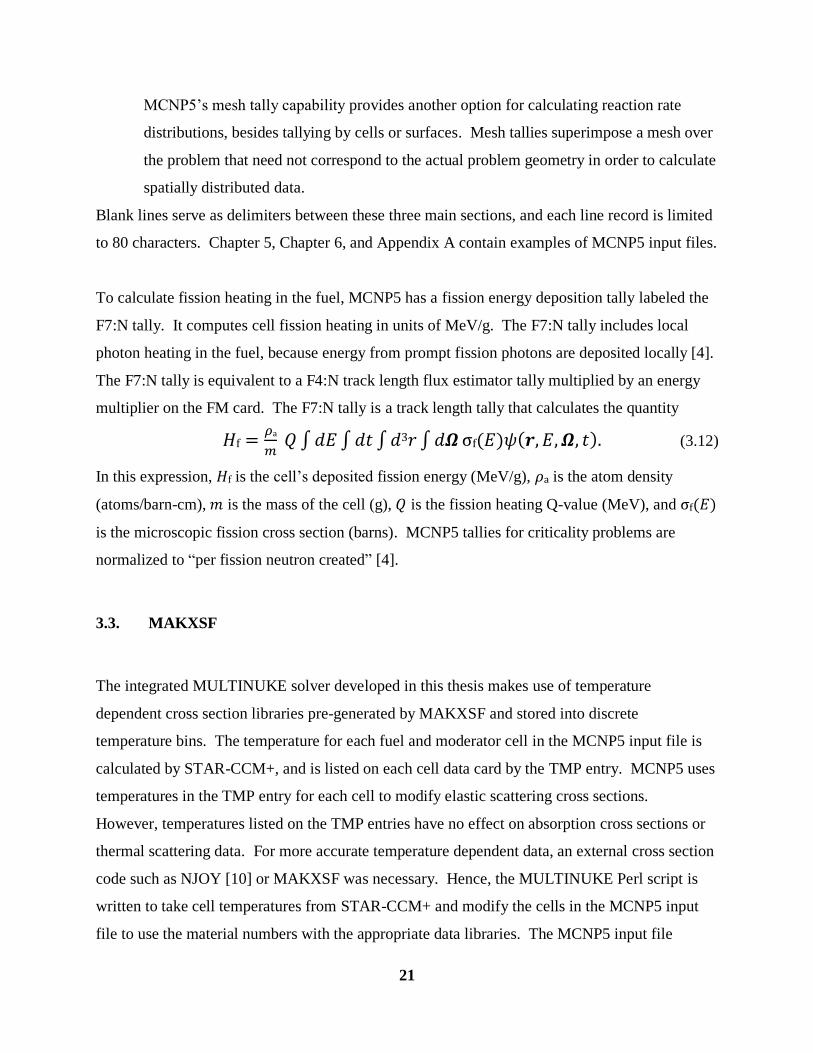
To calculate fission heating in the fuel, MCNP5 has a fission energy deposition tally labeled the
F7:N tally. It computes cell fission heating in units of MeV/g. The F7:N tally includes local
photon heating in the fuel, because energy from prompt fission photons are deposited locally [4].
The F7:N tally is equivalent to a F4:N track length flux estimator tally multiplied by an energy
multiplier on the FM card. The F7:N tally is a track length tally that calculates the quantity
∫ ∫ ∫ ∫ (3.12)
In this expression, is the cell’s deposited fission energy (MeV/g), is the atom density
(atoms/barn-cm), is the mass of the cell (g), is the fission heating Q-value (MeV), and
is the microscopic fission cross section (barns). MCNP5 tallies for criticality problems are
normalized to “per fission neutron created” [4].
3.3. MAKXSF
The integrated MULTINUKE solver developed in this thesis makes use of temperature
dependent cross section libraries pre-generated by MAKXSF and stored into discrete
temperature bins. The temperature for each fuel and moderator cell in the MCNP5 input file is
calculated by STAR-CCM+, and is listed on each cell data card by the TMP entry. MCNP5 uses
temperatures in the TMP entry for each cell to modify elastic scattering cross sections.
However, temperatures listed on the TMP entries have no effect on absorption cross sections or
thermal scattering data. For more accurate temperature dependent data, an external cross section
code such as NJOY [10] or MAKXSF was necessary. Hence, the MULTINUKE Perl script is
written to take cell temperatures from STAR-CCM+ and modify the cells in the MCNP5 input
file to use the material numbers with the appropriate data libraries. The MCNP5 input file

22
contains a number of material numbers for each material (fuel, clad, water) with references to
cross section data ZAIDs at different temperature bins [19].
MAKXSF is capable of altering data file formats, copying and moving data libraries, and
creating nuclide datasets at new temperatures. MAKXSF generates temperature dependent
libraries by using Doppler-broadened resolved resonance data, interpolating unresolved
resonance probability tables, and interpolating S(α,β) thermal scattering kernel data. In order to
modify cross section data to a new temperature, MAKXSF requires two existing cross section
datasets (such as those available in the ENDF/B-VII.0 cross section library). One cross section
dataset must be at a temperature less than desired new temperature, and the second dataset must
be at a temperature greater than the new temperature. MAKXSF has an input file called specs.
The commands to modify cross section datasets to new temperatures are listed in the specs input
file. The command to modify an existing cross section dataset to a new temperature is given by:
ZAIDnew Tnew ZAIDlow ZAIDhigh.
Here, ZAIDnew is the ZAID identifier for the new cross section dataset and Tnew is the new
temperature. ZAIDlow is the existing cross section dataset at a temperature less than Tnew, and
ZAIDhigh is the existing cross section dataset at a temperature greater than Tnew. Every ZAID in
the command must be for the same isotope; thus, the atomic number Z and the mass number A
are the same [19]. For example, the command to generate a new U-235 dataset (Z = 92, A = 235)
at a temperature of 625 K is given by:
92235.01c 625.00 92235.71c 92235.73c
In this command, 92235.01c is the new U-235 ZAID at the new temperature of 625 K. The
ZAID given by 92235.71c designates the cross section dataset for U-235 at 600 K (less than
625 K) from the ENDF/B-VII.0 library. The ZAID given by 92235.73c is the U-235 dataset
at 1200 K (greater than 625) from ENDF/B-VII.0. The complete specs input file used in this
thesis is given in Appendix A.3.
When MAKXSF is executed, it creates and stores the new cross section datasets into a new cross
section library. In the process, MAKXSF creates a new XSDIR directory file, which MCNP5
uses to locate the newly created cross section data [19].

23
Chapter 4. Overview of Computational Fluid Dynamics
Energy is extracted from a reactor by transferring the heat generated by nuclear reactions to a
working fluid. Modeling the coolant behavior in a PWR requires the solution to mass,
momentum, and energy transport equations. In fact, nuclear reactor power output is usually
determined by thermal limitations of reactor materials and coolant. This chapter gives an
overview on the theory of computational fluid dynamics and its use for calculating the thermal-
hydraulic conditions in a PWR. Computational fluid dynamics is a state of the art method for
solving the Navier-Stokes equations in complicated 3D geometries. Prior to CFD, simple
thermal-hydraulic simulations for reactors were generally one-dimensional and used empirical
correlations.
The state of the art code, STAR-CCM+, is used in this thesis for the CFD component of
MULTINUKE. A description of the capabilities and features of the STAR-CCM+ CFD code
follows the discussion of the theoretical basis of CFD codes. Compared to the options for
modeling neutron transport, there are many approaches to representing fluid flow and heat
transfer, and there are many commercially available CFD codes. Therefore, the discussion in
this chapter will be limited to information relevant to STAR-CCM+ and its coupling to MCNP5
for applications involving steady state, turbulent, incompressible flow typical of PWRs. The
governing equations for PWR thermal-hydraulics are presented in their most basic form in order
to illustrate the computational challenge of using high-fidelity methods, such as CFD, for the
analysis of PWR thermal-hydraulics. Although MULTINUKE currently only analyzes steady
state models, the time dependence in the governing equations is retained to fully demonstrate the
complexity of the theory behind PWR thermal-hydraulics.
4.1. Theory
Heat transfer and fluid flow in a nuclear reactor core are difficult to simulate due to the nature of
fluid dynamics phenomena and the geometries involved. The Reynolds number of turbulent
flow in a typical coolant channel ranges from 10,000 to 100,000 [17]. Traditional thermal-

24
hydraulic methods, especially with neutronic coupling, usually are based on simplified one-
dimensional treatments that rely heavily on empirical correlations. Simple thermal-hydraulic
methods use one-dimensional coolant channels divided into relatively large nodes or control
volumes. Mass, momentum, and energy are conserved over each of these large size cells. To
model an entire PWR core, such simple thermal-hydraulic methods are applied to a number of
representative coolant channels, all with unique axial power distributions determined using a
neutronic code. The resulting temperature and density profiles are then input back into the
neutronics solver, with updated cross sections, and the process is repeated iteratively until a
converged solution is obtained [5, 6, 7]. These simple thermal-hydraulic methods only yield
information averaged over the cross section of the fuel assembly.
Computational fluid dynamics is a state of the art method for thermal-hydraulics analysis. For
reactor analysis, it entails discretizing and solving the Navier-Stokes equations over the domain
of the reactor. The geometric domain is discretized into a mesh, and the conservation equations
are solved using finite difference, finite element, or finite volume discretization methods. In a
direct numerical solution (DNS), the Navier-Stokes equations are solved without the use of any
turbulence modeling assumptions; hence, the spatial scale of the computational mesh must be
fine enough to capture the scales of turbulence effects. A direct numerical solution for reactor
applications is a daunting task, even with modern petascale computing. It involves solving for
~1016
unknowns in the governing equations for a time-independent solution, a more formidable
task than deterministic neutronics (1015
unknowns) [2]. Fluid flow in nuclear reactors is highly
turbulent. Turbulence modeling and the nonlinear nature of the momentum transport equation
make the modeling of reactor thermal-hydraulics a challenge. In BWRs, science-based
descriptions of critical heat flux and two-phase flow are difficult, and empirical correlations have
traditionally been used to model such processes [17].
The governing mass and momentum equations for single-phase flow are given respectively by
(4.1)
(4.2)

25
In the momentum equation (4.2), the term
gives rise to the nonlinear nature of
the Navier-Stokes equations, and is a source of some of the computational challenge of PWR
thermal-hydraulics [20]. In these equations, is velocity, is density, is the body force per
unit of fluid mass, and is the stress tensor. For an incompressible Newtonian fluid, the Navier-
Stokes equations are [21]:
(4.3)
(
) (4.4)
(
) (4.5)
The time derivatives vanish for the steady state applications studied in this thesis. In these
equations, is temperature, is pressure, is the specific heat capacity at constant pressure,
is thermal conductivity, is a volumetric heat source in the fluid (such as gamma or neutron
heating), and is the dissipation function. The energy equation above neglects any radiation
heat fluxes. For general three-dimensional flows where the governing equations are coupled, an
equation of state in the form ) must be specified for the fluid. The equation for heat
conduction in the solid fuel and clad regions can be deduced from equation (4.5) and is given by
(4.6)
In equation (4.6), is a volumetric heat source such as fission heating in the fuel or
neutron/gamma heating in the clad. In this thesis, in the fuel region is one of the primary
means of coupling STAR-CCM+ to MCNP5, because MCNP5 generates the volumetric fission
heat source for STAR-CCM+. Neutron and gamma heating are neglected in the cladding, thus
for the clad region in this thesis.
As mentioned before, the discretization of the governing equations (4.3 - 4.6) over the domain of
a PWR core results in ~1016
unknowns for a time-independent DNS. Therefore, turbulence
models are necessary to reduce the computational burden of CFD for PWR applications,
especially when CFD is coupled to Monte Carlo neutronics.
Turbulence modeling is a major challenge, including for PWR thermal-hydraulics. A variety of
turbulence models have been developed for modern CFD methods. Higher fidelity turbulence

26
models are generally more computationally expensive, since they must use smaller scales to
capture the fine scale effects of turbulence. Usually requiring lower computational expense, the
Reynolds-averaged Navier-Stokes (RANS) equations can describe the average effects of
turbulence for complex geometries, where closure is given by models such as k-ε or k-ω models.
A superior method to RANS is the large-eddy simulation (LES) method, where only large-scale
turbulence is solved for explicitly, while the effect of small-scale eddies is modeled. However,
the higher computational costs of large-eddy simulations can limit their application to simple
geometries. Hybrid methods (combining features of RANS and LES), such as the detached-eddy
simulation (DES) model, provide more accurate results than RANS methods while being
computationally quicker than LES methods. LES and DES models require the use of a
computational grid of sufficient resolution, and their higher accuracy solutions should justify
their slower computation times. The second-order closure model, the Reynolds Stress Transport
model (RST or RSM), is a RANS method that directly computes Reynolds stresses instead of the
eddy viscosity approach. RST models are quite accurate but computationally slow [22].
4.2. STAR-DESIGN
STAR-DESIGN is a utility program included with STAR-CCM+ to facilitate CFD geometry
creation, meshing, and solution. It is intended to assist new users in getting started with using
STAR-CCM+. For this thesis, STAR-DESIGN was primarily used for its CAD abilities.
Different regions of a geometric model, such as fuel, clad, and coolant are created separately in
STAR-DESIGN. STAR-CCM+ imports the STAR-DESIGN geometries, and generates the
computational grid (a STAR-CCM+ volumetric mesh). The STAR-DESIGN GUI is capable of
meshing and executing the STAR-CCM+ solver, but with less functionality than the main
STAR-CCM+ GUI. Since STAR-DESIGN is primarily a CAD code intended to assist a new
user in learning STAR-CCM+, the user has less control over mesh options and physics modeling
[22].

27
4.3. STAR-CCM+
STAR-CCM+ is the thermal-hydraulic component of the MULTINUKE integrated solver.
STAR-CCM+ is a commercially available computational fluid dynamics code developed by CD-
adapco. It features an elaborate graphical user interface to facilitate model creation, meshing,
solver execution, and post-processing of data. STAR-CCM+ has a macro feature that records
user GUI actions and automatically creates a Java-based file to reproduce the steps. This feature
is used to run STAR-CCM+ without the GUI (in batch mode), and to assist with data
input/output for repeated runs. For coupled physics with MCNP5, the external-data-table
feature is used to input the volumetric fission heating rate into STAR-CCM+ (in W/m3). This
heat source, called an energy source in STAR-CCM+, is a text data file that lists fission heat
generation rate at each MCNP5 cell centroid. With support from Java macros, STAR-CCM+
automatically reads in each centroid coordinate (x, y, z) and the volumetric heat source
(calculated using MCNP5), and applies the data to the nearest STAR-CCM+ fuel cell. The
energy source from MCNP5 could also have been linked to STAR-CCM+ by user code,
available in C and FORTRAN languages [22].
STAR-CCM+ models fluid flow and heat transfer, as well as heat transfer in solids, in complex
three-dimensional geometries. It solves the Navier-Stokes equations discretized using the finite-
volume approach for steady state and time-dependent problems. STAR-CCM+ can represent
solid, liquid, gaseous, and porous media. Porous media models are especially useful for
representing spacers and flow mixers in nuclear fuel assemblies when full geometric models of
such structures are not required. Heat may be transferred via conduction, radiation, and
convection. STAR-CCM+ models both single and multi-phase flow, with the ability to model
boiling and cavitation phase changes. The code can solve the governing equations
simultaneously (coupled), or in a segregated fashion more appropriate for simpler incompressible
and isothermal flows. The coupled flow solver is more rigorous and accurate, and it can employ
either implicit integration or explicit integration using a Runge-Kutta multi-stage scheme [22].
Surface and volume meshes can be created using STAR-CCM+, or imported from other software
in a variety of formats. Meshing in STAR-CCM+ is highly automated, but allows substantial

28
user control if desired. The overall resolution of a finite-volume mesh is user controlled. Mesh
cells can be manipulated by scaling, translating, rotating, splitting, combining, or deleting. The
surface remesher and surface wrapper can improve a surface mesh for a better finite-volume
grid. STAR-CCM+ can generate tetrahedral, polyhedral, and trimmed (hexahedral) meshes.
Prism layers of mesh cells can be included for modeling heat transfer and turbulence at important
surfaces. STAR-CCM+ also features automatic tools for checking the quality and validity of a
volume mesh [22].
STAR-CCM+ features a host of turbulence models – the most complex and slow being the
Reynolds stress transport model [22]. Some of the available turbulence models include:
Models that provide closure to the Reynolds-averaged Navier-Stokes (RANS) equations
o k-epsilon (k-ε)
o k-omega (k-ω)
o Reynolds stress transport model (RST/RSM)
Large-eddy simulation (LES)
Detached-eddy simulation (DES)
Wall treatments

29
Chapter 5. MULTINUKE Solver
MULTINUKE is an integrated set of computer codes. Developed as part of this thesis, it
automates the coupling of neutronic and thermal-hydraulic solutions for steady state PWR
simulations. It is comprised of MCNP5, STAR-CCM+, a master Perl script, and Fortan90 and
Java data management programs. MULTINUKE needs cross section data pre-generated using
NJOY or MAKXSF in order to include fully temperature dependent neutronics. The code runs
serially or in parallel mode, since both MCNP5 and STAR-CCM+ have built-in parallel
capabilities. The techniques and procedures implemented in MULTINUKE for PWR thermal
feedback calculations are described in Section 5.1. Next, the manual preparations required to use
MULTINUKE are described in Section 5.2. This includes MCNP5 and STAR-CCM+ model
creation, mesh interpolation, and input file formats.
5.1. MULTINUKE Automated Solver
5.1.1. MULTINUKE Perl Script Processes
MULTINUKE automatically executes MCNP5 and STAR-CCM+ in a cyclical fashion,
exchanging data through ASCII data files. Figure 1 illustrates the order of the primary
MULTINUKE procedures. To begin the process, MULTINUKE reads the multiSpecs_base.txt
input file and the mesh correlation files (these files are described in Section 5.2.3 and Section
5.2.4). It then creates an isothermal MCNP5 input file, with initial cell temperatures at a user
specified value, and runs an isothermal MCNP5 calculation that tallies an initial fission energy
distribution. After each neutronic calculation, MULTINUKE calls the Fortran90 post-processor,
GETHEAT, to extract and normalize tally data from the MCNP5 output file. GETHEAT creates
the data file Heat_n.xy (n is the MULTINUKE iteration number) that contains centroid and heat
source information for each cell. MULTINUKE also extracts the eigenvalue from the MCNP5
output file for monitoring convergence of the coupled solution. GETHEAT is described in detail
in Section 5.1.2.

30
Figure 1. MULTINUKE Solver Processes.
Files Created at Each Step
MCNP5 isothermal input file
MCNP5 isothermal output file
Heat_0.xy
STARCCMfuel_out_n.csv
STARCCMwater_out_n.csv
STARCCMclad_out_n.csv
MCNP5 input file for iteration n
MCNP5 output file for iteration n
Heat_n.xy
convergenceSummary.txt
Execution of MULTINUKE Perl script
Run GETHEAT: Fortran90 post-processor to extract power distribution (W/m3) in a format readable by STAR-CCM+. Create Heat_0.xy file.
Run Java script that executes STAR-CCM+ and reads in MCNP5 energy source (W/m3). Output temperature and density data for fuel, clad, and water regions in the form of CSV files. (Begin convergence loop.)
Extract data from STAR-CCM+ CSV files and apply the data to appropriate MCNP5 cells in a new MCNP5 input file.
Run MCNP5 and GETHEAT post-processor.
Read multiSpecs_base.txt input and mesh correlation files, create isothermal MCNP5 input file, and execute MCNP5 isothermal job.
Check for neutronic and thermal-hydraulic convergence: calculate eigenvalue and temperature convergence parameters.
Loop until convergence criteria are satisfied, or until maximum iteration count is reached.
1
2
3
4
5
6
7

31
After the isothermal neutronic calculation, the solver enters a loop that terminates once the
solution converges. The loop begins with MULTINUKE executing the STAR-CCM+ Java
script. The Java script initiates the STAR-CCM+ simulation file by reading in the data from
Heat_n.xy and applying the fission energy source to the fuel region of the model. STAR-CCM+
automatically allocates heat generation rate data from each MCNP5 cell to the appropriate
STAR-CCM+ cell. This is accomplished by calculating the minimum distances between the
MCNP5 centroids in the Heat_n.xy file and the centroids in the CFD simulation file. Finally, the
Java script runs the CFD solver in STAR-CCM+ and generates output files in CSV format.
These CSV files contain cell index, temperature, density, and centroid data for all cells in the
STAR-CCM+ model. These CSV (output) files are named STARCCMfuel_out_n.csv,
STARCCMwater_out_n.csv, and STARCCMclad_out_n.csv (n is the iteration number). After
each STAR-CCM+ run, the Perl script in MULTINUKE calculates the average percent
difference in cell temperatures between subsequent iterations. A description of the processes
performed by the STAR-CCM+ Java script is given in Section 5.1.3, and development of the
Java script is described in Section 5.1.2.
The MULTINUKE Perl script extracts the cell indices, temperature, density, and centroid
information from STAR-CCM+ output files. With the cell indices related by the mesh
correlation files, MULTINUKE creates a new MCNP5 input file. Each MCNP5 cell’s material
(and associated temperature dependent cross section libraries), temperature, and density (if
moderator) are updated by the Perl script during the creation of each new MCNP5 input file.
Once again, MULTINUKE executes MCNP5 and then the GETHEAT post-processor. The
process of alternating between CFD and neutronic solutions is repeated until the eigenvalue and
temperature distributions converge. Figure 2 provides a simple illustration that summarizes
MULTINUKE’s data exchange process and the various programs involved. The Perl source
code can be found in Appendix B.1.

32
Figure 2. MULTINUKE Programs and Data Exchange.
5.1.2. GETHEAT – MCNP5 Post Processor Calculations
After each neutronic calculation, MULTINUKE runs the MCNP5 post-processing code
GETHEAT. This Fortran90 program reads multiSpecs_base.txt to get the name of the MCNP5
input file, and to obtain information necessary for converting MCNP5 tally data into a STAR-
CCM+ heat source (in W/m3). MCNP5 normalizes tallies in criticality mode by the fission
neutrons generated, and the F7:N heat deposition tally is in unit of MeV/g. Therefore,
GETHEAT calculates a constant multiplier that is applied to F7:N tally data to obtain the heat
generation rate in units of W/m3. The multiplier depends on the number of neutrons released per
fission, power level, and keff. The number of neutrons released per fission ( ) and keff vary with
each MCNP5 iteration in a single MULTINUKE run, thus the tally multiplier is updated after
each MCNP5 execution. GETHEAT extracts keff, , and tally data from the MCNP5 output file.
The equation for calculating fission energy in correct STAR-CCM+ units is given by [4, 24, 25]:
MULTINUKE Perl script: exchanges data and
executes codes
Thermal-hydraulics: STAR-CCM+ and Java
Script
Neutronics: MCNP5, GETHEAT, and MAKXSF
CFD mesh indices,
centroids, volumes,
temperatures, and densities.
Neutronic mesh indices,
centroids, volumes, and
power densities (W/m3).
Computational grids
linked by mesh
correlation files.

33
*
+
( -
)
[ ] (
) ( -
) (5.1)
In equation (5.1), *
+ is the real fission power density deposited in each fuel cell, and
[ ] is the normalized tally data directly from the MCNP5 output file. is the system’s
power level in Watts, is the average number of neutrons released per fission, is the energy
released per fission (MeV), and is the fuel density (g/cm3). This equation accounts for
MCNP5 tally normalization and converts the resulting MeV/g data into W/m3 data. *
+ is the
quantity printed out for each cell in the Heat_n.xy data file. Appendix B.2 contains the source
code of GETHEAT.
5.1.3. STAR-CCM+ Java Script
The STAR-CCM+ Java script, loadHeat_runStarJob_base.java, is edited by the MULTINUKE
Perl script before each thermal-hydraulic calculation. With the working directory and current
iteration number obtained from the MULTINUKE Perl script, the Java script loads the Heat_n.xy
file and applies the fission power density to the fuel region in the CFD model, executes the
STAR-CCM+ solver, and writes thermal-hydraulic results in files in CSV format for the
subsequent neutronic calculation. The Java script also allows STAR-CCM+ to be run without
using the graphical user interface (batch mode). MULTINUKE and the Java script do not
modify the STAR-CCM+ base simulation file. Each CFD run uses the same base simulation file
and saves the results in a new file indexed by the iteration number. Manual preparation of the
Java script is described in Section 5.2.2. Appendix B.3 contains the source code of the STAR-
CCM+ Java script.
5.2. Solver Preparation
Although MULTINUKE automatically exchanges heat generation rate, temperature, and density
data, the code requires some manual preparation. Before the MULTINUKE is executed,
MAKXSF pre-generates tables of temperature dependent neutron transport data, including
thermal S(α,β) tables, over a temperature range appropriate for PWR temperatures. Likewise,
34
STAR-CCM+ and MCNP5 models prepared for MULTINUKE contain specific facets for
neutronic–thermal-hydraulic coupling. Finally, input files used by MULTINUKE are to be
prepared to simulate the desired PWR model.
5.2.1. MCNP5 Input File Preparations
In order for MULTINUKE to couple MCNP5 to STAR-CCM+, the fuel and moderator regions
described in the MCNP5 input file need to be divided into small cells that correspond to the CFD
mesh. Additionally, each cell card in the input file needs to be specifically formatted so that
MULTINUKE can modify the neutronic model with updated thermal-hydraulic data. The
MULTINUKE Perl script requires that the MCNP5 input file contain unique “dummy” character
string designators in cell data cards (where there would normally be real data), so that it may
locate and edit the material, temperature, and density (if H2O) of each cell. This necessitates the
creation of an MCNP5 “base” input file, which is an actual MCNP5 input file with cell data
replaced with character strings. When the MULTINUKE Perl script is executed, it locates and
replaces the character strings in the base input file with appropriate data, and creates a real
MCNP5 input file for the next neutronic iteration. Specifically, MULTINUKE looks for
“f_####” for fuel material numbers, “ft####” for fuel temperatures, “w_####” for moderator
material numbers, “wden_####” for moderator densities, “wt####” for moderator temperatures,
“mclad” for clad material number, and “cladt” for cladding temperature (#### is a 4 digit cell
index). Below, Figure 3 shows examples of base input data for fuel, water, and clad cells. Note
that solid material densities (fuel and clad) are assumed to be constant. The cell data in the base
input file must fit within the 80-column MCNP5 limit.

35
Figure 3. Sample MCNP5 Base Input File Excerpt.
MCNP5 input files are developed to represent an accurate model of a PWR core at steady state
conditions. Currently, MULTINUKE is intended to only analyze steady state PWR problems.
[However, MULTINUKE can be used to analyze any nuclear reactor with a single-phase
coolant, such as liquid metal cooled reactors with fast neutron spectra. Only the cross section
database would require significant alteration.] In order to tally reaction distributions and
exchange data with STAR-CCM+, the fuel and moderator regions of the model are divided into
several smaller cells, corresponding to mesh cells in the CFD grid. The cladding regions of the
model may also be built of many small cells, but the cladding temperature distribution is not as
significant as fuel and moderator temperatures for thermal feedback. There is essentially no

36
limit to the size of the model – it could range from a single pin to an entire core. Computer
limitations determine the maximum size of the MCNP5 model.
Fission heat generation rate, or flux modified to calculate fission heating, is tallied over MCNP5
cells. By tallying over several cells, MULTINUKE calculates reaction rate distributions from
MCNP5 output files. Tallying by cells allows MCNP5 to store heat generation rate, temperature,
and density (if a moderator cell) data for each cell that corresponds to its equivalent cell in the
CFD mesh, thereby facilitating code coupling. In MCNP5, heat generation rate is most easily
calculated using the F7:N fission energy deposition tally. The F7:N tally may require the cell
masses to be listed on tally data cards (SD cards) in the MCNP5 input file, because MCNP5 does
not automatically calculate masses for asymmetric cells. The F7:N tally computes fission
heating in units of MeV/g. Hence, the tallied heating value must be converted to STAR-CCM+
energy source units (W/m3). The details have already been described in Section 5.1.2.
There should be a list of reactor material numbers in the data card section of the MCNP5 input
file containing references to the pre-generated data libraries. Each material number corresponds
to a particular reactor material at a certain temperature. Therefore, each reactor material (UO2,
Zirc, and H2O) will have several material numbers referencing cross section library ZAIDs
generated at different temperatures.
5.2.2. STAR-CCM+ Model Preparations
MULTINUKE requires an appropriate CFD model of the core (or part of the core) of a
pressurized water reactor. The CFD mesh needs to be sufficiently fine for accurate fluid flow
and heat transfer simulation, while being simple enough to “link” with MCNP5 geometry cells.
This means that complex, unstructured polyhedral meshes are not appropriate for use with
MULTINUKE without additional processing of mesh data. Complex CFD meshes that lack
axial symmetry (with cells at various orientations) are very difficult to model in MCNP5.
Therefore, the STAR-CCM+ model should use a relatively simple mesh – most importantly one
that is axially uniform (meaning each axial segment has the same radial mesh structure). When
there is a pattern to the mesh structure, simple scripts or programs can create MCNP5 cell input,
even when there are several thousand cells. The two meshes should have cells with very similar

37
volumes and centroids to allow for accurate data exchange. Without simple meshes and the
automated creation of MCNP5 input files, the grid used for MCNP5 tallies would need to be
axially simplified, as was done in the work of Seker et al. with McSTAR [11].
Mesh compatibility and transfer of data from one code to another are long recognized to be some
of the most challenging steps in externally linked multi-physics problems. Current work linking
MCNP5 and STARCCM+ is based on the premise that the meshes are simple and compatible.
An additional layer of code between MCNP5 and STARCCM+ that interpolates and averages
data from the mesh in one code, to be suitably used by a very different mesh in the other code,
will allow significantly different meshes to be used by the two codes. However, this is expected
to add a significant computational cost.
Once a simple mesh is in place for a PWR core model, the macro feature in the STAR-CCM+
GUI can be used to record a Java macro that performs the following actions:
1. Read in the MCNP5 heating data in the form of an external data table, and apply it to the
fuel region as an energy source term. STAR-CCM+ software can automatically assign
each MCNP5 cell’s heating value to the appropriate CFD mesh cell, since the heating
data file (Heat_n.xy) contains the centroid coordinates of each MCNP5 cell. (This data
exchange should be accurate if the MCNP5 and STAR-CCM+ meshes are identical, or
very similar.)
2. Execute the STAR-CCM+ solver for a sufficient number of CFD iterations (typically
3000-4000 for small PWR problems presented in this thesis).
3. Output the temperature and density of each cell, along with CFD mesh cell index and
centroid coordinates.
After STAR-CCM+ creates the file for the Java macro, the absolute directories in the Java code
are replaced with the character string “_WORKDIR_”. This allows the Perl script to identify the
location for the directory names and update the working directory name each time
MULTINUKE is executed. As described in Section 5.1.1, the Perl script executes the Java
macro in the convergence loop for each MULTINUKE iteration (see step 4 in Figure 1). The
Perl script looks for the file called loadHeat_runStarJob_base.java; it updates the Java code in
this file with the current working directory and iteration number for file management purposes.

38
Then, the Perl script creates a new Java macro file that is actually executed, labeled
loadHeat_runStarJob.java (that has current directory and iteration number). Execution of the
Java macro controls the data input, solver execution, and data output for STAR-CCM+.
5.2.3. Relating the MCNP5 and STAR-CCM+ Meshes
The creation of similar MCNP5 and STAR-CCM+ meshes is straightforward, given a simple
enough grid structure. However, STAR-CCM+ does not index the mesh cells conveniently for
automated MCNP5 input file creation. Thus, the neutronic and CFD meshes will typically be
indexed differently. Relating the indices of the MCNP5 mesh to indices of the STAR-CCM+
mesh is a manual preparatory task of upmost importance.
A simple pattern for numbering the cells in the MCNP5 input file is therefore used to write
scripts to produce large blocks of MCNP5 input deck, such as with Fortran “DO” loops. For the
PWR cell models discussed in Chapter 6, the cell data in the MCNP5 input file is created using
two “DO” loops in a very simple Fortran90 code. The MCNP5 cells are numbered (starting from
cell number 1) left-to-right in the x-direction and bottom-to-top in the y-direction. After the cell
input for an entire axial level is written, this cell-numbering scheme continues in the same
fashion for the next axial node. The x, y, and z surfaces that bound the MCNP5 cells are also
numbered in an appropriate (sequential) manner for writing large blocks of MCNP5 input using
Fortran90 code. The cell-numbering scheme for the MCNP5 input file is apparent in Appendix
A.1, which provides excerpts of the MCNP5 input file used for the single PWR cell simulation
described in Chapter 6. The MCNP5 input file for the 3 x 3 PWR cell model is very similar, but
substantially longer.
When the MULTINUKE Perl script is executed, it looks for the files
fuel_STARcell_equals_MCNPcell.txt and water_STARcell_equals_MCNPcell.txt. These files are
required for data coupling in MULTINUKE. The mesh correlation files are formatted as
“STARcell# = MCNPcell#,” as shown below in Figure 4. To find the relationship between the
mesh indices, one can manually examine both mesh data and match each appropriate cell. Since
this can be excessively time consuming for large meshes, a simple script or program can find the
minimum distances between each cell in the two meshes. If the meshes are nearly identical, zero

39
distance (or nearly zero) should separate the correct cell pairs between the meshes. The program
can then generate the mesh correlation files with cells paired by minimum distance. In this
thesis, the CFD and neutronic meshes for the PWR simulations (in Chapter 6) are correlated by a
simple Fortran90 code that associates mesh cells by minimum distance.
Figure 4. Mesh Correlation File Format Excerpt.
5.2.4. MULTINUKE Input File
The primary MULTINUKE input file, called multiSpecs_base.txt, is edited prior to executing the
coupled codes. The input file multiSpecs_base.txt contains the job name of the problem (the file
name of the MCNP5 and STAR-CCM+ simulation files). It also specifies the nuclear fuel
density (g/cm3), power rating (Watts), energy released per fission event (MeV/fission), iteration
convergence parameters, initial neutronic isothermal temperature (K), and the starting cell index
of the moderator in the MCNP5 input file. MULTINUKE solutions are considered converged
when MCNP5 keff values and STAR-CCM+ cell temperatures change less than a user-specified
tolerance between two consecutive iterations. The multiSpecs_base.txt file contains data input
for the eigenvalue tolerance, and another tolerance level for average percent difference for cell
temperatures. The MULTINUKE code terminates when both convergence criteria are satisfied
in two successive MCNP5–STAR-CCM+ iterations. Some editing of the MULTINUKE Perl
script and data processing programs may be needed when simulating reactors that diverge
significantly from the PWR models simulated in this thesis. Figure 5 shows sample input data in
multiSpecs_base.txt. MULTINUKE extracts parameters for the model by searching for the
keywords, which can be in any order, to the left of the equal sign. The program terminates if a
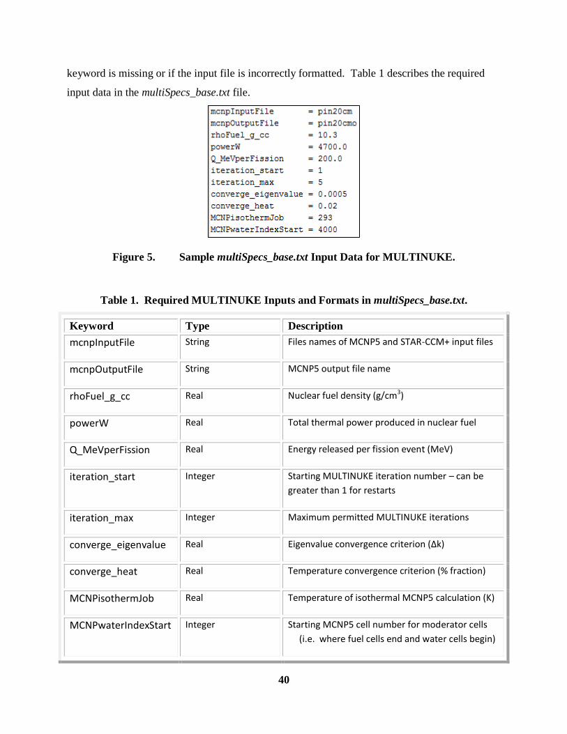
40
keyword is missing or if the input file is incorrectly formatted. Table 1 describes the required
input data in the multiSpecs_base.txt file.
Figure 5. Sample multiSpecs_base.txt Input Data for MULTINUKE.
Table 1. Required MULTINUKE Inputs and Formats in multiSpecs_base.txt.
Keyword Type Description
mcnpInputFile String Files names of MCNP5 and STAR-CCM+ input files
mcnpOutputFile String MCNP5 output file name
rhoFuel_g_cc Real Nuclear fuel density (g/cm3)
powerW Real Total thermal power produced in nuclear fuel
Q_MeVperFission Real Energy released per fission event (MeV)
iteration_start Integer Starting MULTINUKE iteration number – can be
greater than 1 for restarts
iteration_max Integer Maximum permitted MULTINUKE iterations
converge_eigenvalue Real Eigenvalue convergence criterion (Δk)
converge_heat Real Temperature convergence criterion (% fraction)
MCNPisothermJob Real Temperature of isothermal MCNP5 calculation (K)
MCNPwaterIndexStart Integer Starting MCNP5 cell number for moderator cells
(i.e. where fuel cells end and water cells begin)

41
Chapter 6. PWR Test Calculations
The MULTINUKE solver is applied to a single cell model and a 3 x 3 lattice model to
investigate the steady state, coupled neutronics and thermal-hydraulics of a PWR representative
cell. The PWR models are run on a 64 bit, quad core, Intel 2.8 GHz microprocessor with 1 GB
RAM. The MCNP5 source code is compiled and a Linux MPI executable is generated for
parallel neutronics. STAR-CCM+ is released fully capable of parallel processing, and is
executed in parallel mode on the machine’s four cores. The PWR models and the coupled
nuclear and thermal-hydraulic results calculated using MULTINUKE are described below.
6.1. PWR Cell Model Description
The PWR cell model consists of a cylindrical fuel rod (fuel, cladding) surrounded by the coolant
contained within boundaries in the x and y directions. With symmetric boundary conditions
imposed in the x and y directions, the PWR cell model simulates a PWR core as an infinite array
of identical fuel cells. However, the model is finite in the axial direction, allowing axial neutron
leakage and coolant to flow in and out of the model. Figure 6 illustrates the single pin model.
The purpose of the simple PWR cell model is twofold: to debug various functionalities of
MULTINUKE using a problem that runs fast, and to calculate pseudo-realistic PWR conditions
using coupled neutronics/thermal-hydraulic simulations. Although coupled, multi-physics
reactor simulations are intended to analyze large complex models on massively parallel
computing platforms, and MULTINUKE is envisioned for this purpose, the single cell model is
meant to demonstrate the usage of MULTINUKE on a quad core machine. Therefore, the
number of mesh cells in the model is held to a minimum by reducing the height of the model to
20 cm. This allows STAR-CCM+ to generate a simple prismatic hexahedral CFD mesh with
only 9,984 computational cells, which consequently facilitates the creation of an equivalent
neutronic mesh in MCNP5 (excluding the clad region that is lumped into one MCNP5 cell). All
axial nodes have the same radial mesh structure.

42
Figure 6. PWR Cell Model.

43
Table 2 contains important data for the PWR cell model, and subsequent mesh and simulation.
The fuel diameter is 1.0 cm, and the outer clad diameter is 1.2 cm, resulting in a 0.1 cm cladding
thickness with no fuel-clad gap modeled. The lattice has a pitch of 1.5 cm and an axial height of
20.0 cm. The nuclear fuel material is UO2 with 5 w/o U-235 enrichment. Cladding is made of
Zircaloy-4 and liquid water is the coolant and neutron moderator.
Table 2. PWR Cell Model Data.
Lattice Data Value
Fuel Outer Diameter (cm) 1.0
Fuel Cladding Outer Diameter (cm) 1.2
Fuel Cladding Thickness (cm) 0.1
Fuel Rod Pitch (cm) 1.5
Axial Height (cm) 20.0
Fuel Material UO2
Fissile Material Enrichment 5 w/o U-235
Cladding Material Zircaloy-4
Coolant/Moderator Material Liquid H2O
Mesh Data Value
Mesh Type Prismatic Hexahedral
Total STAR-CCM+ Cells 9,984
Number of Radial STAR-CCM+ Cells per Axial Node 96
Number of STAR-CCM+ Axial Nodes 104
Total MCNP5 Cells 7488 + 1 Clad Cell
Number of Radial MCNP5 Cells per Axial Node 72
Number of MCNP5 Axial Nodes 104
Number of MCNP5 Tally Regions (UO2 Cells) 3328
6.1.1. Computational Grid
STAR-DESIGN is used to create CAD geometries of the fuel, clad, and coolant regions of the
PWR cell model. These are then imported into STAR-CCM+, which is used to generate the
volumetric computational mesh. The resolution of the mesh automatically generated by STAR-
CCM+ is determined by the surface mesh and the size of the model. For a long and slender CFD
geometry, such as a lattice cell, the axial length determines the mesh size since it is the longest
dimension of the model. To generate the surface mesh, the surface mesh size is specified to be
1% of the axial length. With the surface mesh generated, STAR-CCM+ automatically creates
the volumetric mesh where base computational cell size is specified to be 1% of the length of the
model. A 3D view of the surface mesh used to create the volume mesh is shown in Figure 7.

44
Figure 7. CFD Surface Mesh for Single PWR Cell.
An axially uniform mesh is desired to facilitate coupling with the neutronics mesh; thus, a
prismatic hexahedral CFD mesh is generated using the “trimmer” mesh model option in STAR-
CCM+. The trimmer option can generate better quality meshes than the STAR-CCM+
tetrahedral mesher, needing five to eight times less number of cells for the same accuracy [22].
Trimmed meshes also lead to better quality volumetric meshes than the polyhedral mesh model
when the surface mesh is low quality. A summary of mesh data for the PWR cell model is given
in Table 2. The model has 96 radial CFD cells per axial node, with 104 axial nodes, resulting in
9,984 CFD computational cells. An equivalent neutronic grid is created in MCNP5 with help
from a simple Fortran90 program. The MCNP5 computational cells have almost identical
centroids and volumes compared to the STAR-CCM+ cells, except for the clad region that is
reduced to one cell in the MCNP5 input file. The cladding temperature for MCNP5 is calculated
as the volume weighted average of the STAR-CCM+ clad cells’ temperatures. The MCNP5
model has 7,489 computational cells, including 3,328 tallied fuel cells. Figure 8 and Figure 9
depict the STAR-CCM+ mesh and MCNP5 mesh, respectively. The upper-right quadrant of the
coolant mesh is numbered for the results presented in Section 6.2.8 (see Figure 28).

45
Figure 8. STAR-CCM+ Mesh for PWR Cell Model.
Figure 9. MCNP5 Geometry Cells for PWR Cell Model.
1 2 3 4
5 6 7
8 9
10

46
6.1.2. MAKXSF Pre-generated Cross Section Data
Prior to execution of MULTINUKE, MAKXSF is run to pre-generate cross section data over a
temperature range appropriate for a typical PWR. MAKXSF copies cross section data from
ENDF/B-VII.0 for the initial isothermal MCNP5 calculation. The MAKXSF input file used to
create the cross section data for the PWR cell model is given in Appendix A.3. In order for
MCNP5 to locate the required data, the code is executed for each MULTINUKE iteration using
the command:
mpirun -n 4 mcnp5.mpi n=$JOB_NAME xsdir=xsdir_broad1 .
This command executes the Linux MPI MCNP5 executable over all of the cores of the
machine’s processor. The code also locates the temperature dependent cross section data using
the information in the command line. For the PWR cell model, a temperature dependent library
designated “broad1” is specified for MCNP5 by the XSDIR file called “xsdir_broad1.”
After each STAR-CCM+ calculation, MULTINUKE assigns material numbers to all cells in
MCNP5 by comparing each cell’s calculated temperature to the nearest pre-generated
temperature bin for that particular material. Hence, cells at very different temperatures for the
same material are assigned different material numbers. Tables 3, 4, and 5 list the temperature
bins used by MAKXSF to pre-generate cross section data, along with the associated material
numbers and ZAIDs that are in the PWR cell model’s base MCNP5 input file. (ZAIDs are
explained in Sec. 3.2.) The ID extension refers to the suffix on the ZAID numbers in the
MCNP5 input file. For example, for a UO2 fuel cell that has temperature close to 925 K,
MULTINUKE assigns the material number 7 (with ID suffix “.07c”) to that cell. Material 7
appears in data card section of the MCNP5 input file, as shown in Figure 10.
Figure 10. Example MCNP5 Material Data Card for PWR Cell Model.

47
Table 3. MAKXSF Temperature-Binned Fuel Cross Sections.
Fuel Material Number
MCNP5 ZAID ID Extension Bin Tmin (K) Bin Tmax (K)
Temperature at which Data is Evaluated (K)
1 .01c 600 650 625
2 .02c 650 700 675
3 .03c 700 750 725
4 .04c 750 800 775
5 .05c 800 850 825
6 .06c 850 900 875
7 .07c 900 950 925
8 .08c 950 1000 975
9 .09c 1000 1050 1025
10 .10c 1050 1100 1075
11 .11c 1100 1150 1125
12 .12c 1150 1200 1175
13 .13c 1200 1250 1225
14 .14c 1250 1300 1275
15 .15c 1300 1350 1325
Table 4. MAKXSF Temperature-Binned Cladding Cross Sections.
Clad Material Number
MCNP5 ZAID ID Extension Bin Tmin (K) Bin Tmax (K)
Temperature at which Data is Evaluated (K)
21 .21c 500 600 550
22 .22c 600 700 650
23 .23c 700 800 750
Table 5. MAKXSF Temperature-Binned Moderator Cross Sections.
Coolant Material Number
MCNP5 ZAID ID Extension Bin Tmin (K) Bin Tmax (K)
Temperature at which Data is Evaluated (K)
31 .31c ( .31t for S(α,β) ) 550 560 555
32 .32c ( .32t for S(α,β) ) 560 570 570
33 .33c ( .33t for S(α,β) ) 570 575 572.5
34 .34c ( .34t for S(α,β) ) 575 580 577.5
35 .35c ( .35t for S(α,β) ) 580 585 582.5
36 .36c ( .36t for S(α,β) ) 585 590 587.5
37 .37c ( .37t for S(α,β) ) 590 595 592.5
38 .38c ( .38t for S(α,β) ) 595 600 597.5
39 .39c ( .39t for S(α,β) ) 600 610 605

48
6.1.3. Neutronics Modeling
The nuclear physics of the PWR cell model are treated using steady state, three-dimensional,
Monte Carlo neutron transport. Gamma and neutron heating in the clad and moderator are
neglected; only fission heating and local prompt gamma heating in the fuel are tallied by
MCNP5 in order to create a heat generation rate for STAR-CCM+.
The MCNP5 model has 3328 fuel cells and 4160 moderator/coolant cells, matching the CFD
mesh for the fuel and water regions. The CFD mesh of the clad region is collapsed to a single
MCNP5 cell. The MCNP5 geometry has dimensions identical to the STAR-CCM+ geometry.
After each CFD run, MULTINUKE assigns the appropriate temperature, material number, and
density (if a moderator cell) to the corresponding MCNP5 cells by modifying the MCNP5 base
input deck (the “base” input file for MCNP5 is discussed Sec. 5.2.1).
Reflective boundary conditions are specified on the surfaces in the x and y directions in the
MCNP5 model. Neutron leakage is permitted from the top and bottom axial surfaces. The
simple 20 cm cell model is not representative of any realistic nuclear reactor design. High axial
leakage leads to low keff values of about 0.6 to 0.8. Since the PWR cell model does not have any
axial reflector regions, no reflector power peaking at the top and bottom of the model will be
shown for the results in Section 6.2. The PWR cell model is not a criticality search problem –
but a steady state thermal feedback simulation for a hypothetical PWR.
As discussed in Section 5.1.2, the tallies for heat generation rate are dependent on the eigenvalue
and average neutrons released per fission ( ) (see equation (5.1)). Because remains relatively
constant compared to the reactivity feedback, the overall power level will fluctuate as keff
changes during the iterations. Therefore, the (fission) heat generation rate data transferred to
STAR-CCM+ is scaled by a constant (which is updated after each MCNP5 calculation) to keep
the overall power level equal to the value specified in the MULTINUKE input file,
multiSpecs_base.txt.

49
For the PWR cell simulation, MCNP5 is executed in neutron transport mode (mode n) with no
explicit photon particle transport. Delayed neutrons are accounted for by using the TOTNU data
card in the MCNP5 input file. Each MULTINUKE neutronic calculation ran 160 batches of
neutrons with 15,000 neutron histories in each batch, while discarding the first 10 batches for
proper eigenvalue and fission source convergence. Source neutrons are uniformly distributed
over a cylindrical region that encompasses all fissionable material in the model. There were no
warnings from MCNP5 of unsampled cells containing fissionable material. Figure 11 shows the
MCNP5 physics data card used for the PWR cell model, also showing that default MCNP5
neutron physics are used since special physics options are not specified.
Figure 11. MCNP5 Physics Data Cards for PWR Cell Model.
6.1.4. Thermal-Hydraulics Modeling: CFD Solver
The thermal-hydraulics of the PWR cell model are simulated using single-phase, three-
dimensional, steady state, computational fluid dynamics in conjunction with 3D heat conduction
in solids. The coupled flow solver in STAR-CCM+ (for conjugate heat transfer) is used so that
the governing equations can be solved simultaneously, since it intrinsically provides more robust
solutions. It is advised in the STAR-CCM+ manual to use the coupled flow solver for problems
with large energy sources and if the computational burden is not too high [22]. (The segregated
flow and energy solvers could have been used because the flow is essentially incompressible;

50
however, the presence of the large fission energy source in the fuel region (~108 W/m
3)
necessitates the use of the coupled flow solver.) The PWR model simulates heat conduction in
the solid fuel and clad regions using the coupled solid energy solver in STAR-CCM+. For the
steady state PWR cell model, the coupled flow solver incorporates a pseudo-time marching
approach to solve the governing equations simultaneously. The coupled flow solver uses
implicit-steady integration to solve the discretized equations, providing relatively faster
convergence rates than explicit-steady integration with a multi-stage Runge-Kutta scheme [22].
Table 6 summarizes the parameters used in simulating the PWR cell model using STAR-CCM+.
For the steady coupled solver, the Courant number specifies the maximum size of the local
pseudo-time steps used by the solver when integrating the governing equations. When faced
with convergence difficulties during initial iterations, it may be necessary to decrease the
Courant number. The governing equations are discretized using a second-order discretization
scheme. For the PWR model, a Gauss-Seidel relaxation scheme with a convergence tolerance of
0.01 is used.
Table 6. CFD Solver Options in STAR-CCM+ for PWR Cell Model.
STAR-CCM+ Solver Parameter Value
Solver Type Coupled Implicit
Equation Discretization Method 2nd
Order Upwind
Courant Number 5.0
Relaxation Scheme Gauss-Seidel
Solver Convergence Tolerance 0.01
6.1.5. Modeling Turbulence in the PWR Cell Simulation
The coolant in the PWR cell model is treated as a viscous and turbulent liquid. Turbulence
modeling is accomplished using the realizable two-layer k-ε model that provides closure to the
Reynolds-averaged Navier-Stokes (RANS) equations. The k-ε turbulence method is a two-
equation eddy viscosity model that solves the transport equation for turbulent kinetic energy (k)
and dissipation rate (ε). It usually gives reasonable results for simple models that have a

51
relatively coarse mesh [22]. There are more accurate turbulence models in STAR-CCM+
available for future work with MULTINUKE. In STAR-CCM+, the realizable two-layer k-ε
turbulence model is a combination of the realizable k-ε model and the two-layer turbulence
model.
The realizable two-layer k-ε turbulence model for the PWR model uses the default turbulence
options in STAR-CCM+, some of which are listed in Table 7. The turbulence model uses a
shear driven (Wolfstein) two-layer formulation with an all-y+ wall treatment. The Boussinesq
approximation is used for a linear constitutive relation, which is recommended for all k-ε models
in the STAR-CCM+ manual. The PWR cell model has a second-order convection scheme,
which is superior to first-order convection schemes [22]. The under-relaxation factor of the
turbulence solver is set to 0.8, the default for k-ε turbulence in STAR-CCM+. The turbulence
solver under-relaxation factor affects solution convergence – lowering it may help convergence
but also slows down the solver. The algebraic multigrid (AMG) linear solver values in Table 7
set the parameters for STAR-CCM+ to solve the discretized linear systems of equations in an
iterative fashion. The details on these parameters can be found in the STAR-CCM+ user guide
[22]. With the k-ε viscosity under-relaxation factor set to 1.0 (as shown in Table 7), the entire
turbulent viscosity is updated after each CFD iteration computes a new turbulent viscosity field.
Table 7. CFD Turbulence Options in STAR-CCM+ for PWR Cell Model.
Parameter Value
Turbulence Model Realizable Two-Layer k-ε
Two-Layer Type Formulation Shear Driven (Wolfstein)
Wall Treatment All-y+
Constitutive Relation Linear
Convection Scheme 2nd
Order
k-ε Under-Relaxation Factor 0.8
Algebraic Multigrid Linear Solver Convergence Tolerance 0.1
Algebraic Multigrid Linear Solver Maximum Cycles 30
Algebraic Multigrid Linear Solver Group Size 2
k-ε Turbulence Viscosity Under-Relaxation Factor 1.0

52
6.1.6. Thermo-Physical Material Properties
The thermo-physical properties of the solid UO2 and Zircaloy-4 regions are assumed to be
constant. Still, an effort is made to input solid material data at temperatures appropriate for the
PWR cell model. Table 8 and Table 9 designate the constant material properties for the fuel and
clad regions of the PWR model, and the source from which the data was obtained.
Table 8. UO2 Thermo-Physical Properties for PWR Cell Model.
Thermal Property Value Source of Data and Reference #
ρ, Density (g/cm3) 10.3 Duderstadt, 1976 [6]
k, Thermal Conductivity (W/m-K) 3.0 Argonne National Laboratory [26]
cp, Specific Heat Capacity (J/kg-K) 310 Todreas, 1993 [21]
Table 9. Zircaloy-4 Thermo-Physical Properties for PWR Cell Model.
Thermal Property Value Source of Data and Reference #
ρ, Density (g/cm3) 6.50 Duderstadt, 1976 [6]
k, Thermal Conductivity (W/m-K) 11.0 Argonne National Laboratory [27]
cp, Specific Heat Capacity (J/kg-K) 330 Argonne National Laboratory [28]
The coolant is assumed to have constant thermal conductivity, as well as constant dynamic
viscosity and turbulent Prandtl number. Table 10 gives the water properties chosen from the
stated source at the approximate coolant temperatures of the PWR model. The density and
specific heat capacity of the coolant in STAR-CCM+ are however not constant, but rather
polynomial functions of the cell temperature. The thermal expansion of the coolant is discussed
in the next section.
Table 10. H2O Thermo-Physical Properties for PWR Cell Model.
Thermal Property Value Source of Data and Reference #
μ, Dynamic Viscosity (Pa-s) 9.177x10⁻⁵
El-Wakil, 1993 [5]
k, Thermal Conductivity (W/m-K) 0.53 El-Wakil, 1993 [5]
Pr, Turbulent Prandtl Number 0.90 STAR-CCM+ Manual, 2007 [22]
The specific heat capacity for H2O is modeled by the following temperature dependent equation
in STAR-CCM+:

53
{
(6.1)
In equation (6.1), temperature (T) has units of Kelvin, and the specific heat capacity (cp) has
units of J/kg-K. The polynomial is a fourth-order fit of specific heat data in Nuclear Heat
Transport by M. M. El-Wakil [5]. Figure 12 depicts the H2O heat capacity for the PWR cell
model, where the red curve denotes the heat capacity equation (6.1) and the blue dots are data
from El-Wakil [5]. (The H2O heat capacity is assumed to be constant outside the coolant
temperature range of interest.)
Figure 12. Specific Heat Capacity for Coolant in PWR Cell Model.
y = 5.002E-05x4 - 1.066E-01x3 + 8.515E+01x2 - 3.025E+04x + 4.032E+06 R² = 9.997E-01
4000
4500
5000
5500
6000
6500
7000
450 475 500 525 550 575 600 625 650
Spec
ific
He
at C
apac
ity
(J /
kg-
K)
Temperature (K)
H2O Heat Capacity vs Temperature at 2000 psi

54
6.1.7. Equation of State and Moderator Density
When simulating a single-phase fluid with the steady state, coupled flow solver, STAR-CCM+
allows for constant density, density varying as a polynomial, and ideal gas treatment for the
equation of state. To model the equation of state, STAR-CCM+ simulates the thermal expansion
of coolant in the PWR cell model using a user-specified polynomial fluid density. A user-
specified equation of state is specified making use of the water density data from El-Wakil. The
equation for coolant density as a function of temperature at 2000 psi pressure in the PWR cell
mode is [5]:
{
(6.2)
In equation (6.2), is the H2O density in kg/m3, temperature (T) is in Kelvin and coolant density
is assumed to be constant outside the temperature range of interest for the PWR model. Figure
13 shows the variation of coolant density with temperature. The red curve represents equation
(6.2) and the blue dots are the data points for water density from El-Wakil [5].

55
Figure 13. Water Density Temperature Dependence in PWR Cell Simulation.
6.1.8. STAR-CCM+ Initial Conditions and Boundary Conditions
The STAR-CCM+ simulation file for the PWR model contains three mesh continua and three
physics continua, corresponding to the three geometry regions in the model (“continua” is a
STAR-CCM+ term referring to data input sections in the GUI where mesh data and physical
quantities are specified by the user). The trimmer mesh generator can only generate a hexahedral
mesh for one region at a time; therefore, three mesh continua are necessary for the model. There
exist two interfaces: one between the fuel and clad regions, and one between the clad and
coolant regions. The physics continua specify the material properties of the regions and the
initial conditions for the CFD solver. Table 11 shows the initial thermal-hydraulic conditions for
y = -4.118E-08x4 + 6.740E-05x3 - 4.306E-02x2 + 1.182E+01x - 1.544E+02 R² = 1.000E+00
600
650
700
750
800
850
900
950
1000
1050
250 300 350 400 450 500 550 600 650
Den
sity
(kg
/m3 )
Temperature (K)
Water Density vs Temperature at 2000 psi

56
the PWR model. These initial conditions only serve as the “initial guess” for the steady state
problem.
Table 11. Initial Thermal-Hydraulic Conditions for PWR Cell Model.
Initial Parameter Value
UO2 Fuel Continua Temperature (K) 1000.0
Fuel-Clad Interface Temperature (K) 900.0
Zircaloy-4 Clad Continua Temperature (K) 800.0
Clad-Coolant Interface Temperature (K) 800.0
H2O Coolant Continua Temperature (K) 580.0
H2O Coolant Inlet Temperature (K) 570.0
H2O Coolant Inlet Speed (m/s) 1.0
H2O Coolant Initial Pressure (Pa) 1.55x10⁷
H2O Coolant Exit Pressure (Pa) 1.50x10⁷
Initial Turbulence Specification Intensity + Viscosity Ratio
Turbulence Intensity 0.01
Turbulent Viscosity Ratio 10.0
Symmetry boundary conditions are imposed on the surfaces in the x and y directions in the
STAR-CCM+ simulation file. Inlet velocity is specified at the (bottom) inlet, and a pressure
boundary condition is specified at the top surface. The fuel-clad and clad-coolant interfaces have
continuous boundary conditions. No-slip boundary conditions are specified for the coolant on
the cladding surface.
6.1.9. MULTINUKE Input Data
Assuming the PWR model represents an average fuel pin in a PWR with a power density of
3.00x10⁸ W/m
3, a power rating of 4700.0 Watts is designated in the muliSpecs_base.txt input
file. The UO2 fuel density is selected to be 10.3 g/cm3, and it is assumed that each fission
releases 200 MeV of energy. Rather relaxed MULTINUKE convergence criteria are selected in
order to expedite development and debugging of the coupled code system. Once two successive
iterations yield a difference of less than 0.0005 eigenvalue (Δk) and less than 2% average change
in cell temperatures, the solution is considered to be converged. Simulations can be easily run

57
with more strict convergence criteria. Table 12 contains some important input data for
MULTINUKE to analyze the PWR cell model.
Table 12. PWR Cell Input Data for MULTINUKE.
Input Data Value
Job Name pin20cm
Fuel Density (g/cm3) 10.3
Power Output (W) 4700.0
Q – Energy Released per Fission (MeV/fission) 200.0
Eigenvalue Convergence (Δk) 0.0005
Temperature Convergence (fraction % difference) 0.02
MCNP5 Initial Isothermal Temperature (K) 293
6.2. PWR Cell Model Results
This section discusses the results of neutronic and thermal-hydraulic calculations for the PWR
cell model. MCNP5 and STAR-CCM+ results to validate the neutronic and thermal-hydraulic
models separately are discussed in the first four subsections (6.2.1, 6.2.2, 6.2.3, and 6.2.4).
Results obtained for the coupled MCNP5 and STAR-CCM+ simulations carried out using by
MULTINUKE for the PWR cell model are discussed in the remaining subsections (6.2.5, 6.2.6,
6.2.7, 6.2.8, and 6.2.9).
6.2.1. MCNP5 Eigenvalue and Fission Source Convergence
Sufficient neutron history cycles must be discarded in order for the eigenvalue and fission source
calculated by MCNP5 to properly converge. Figure 14 and Figure 15 respectively depict
convergence of eigenvalue and fission source entropy for a typical MCNP5 simulation of the
PWR model. MCNP5 is run with 15,000 neutron histories per cycle for 160 total cycles, while
discarding the first 10 batches, for every MCNP5 calculation in MULTINUKE. The cycle
discard number is shown at the tenth cycle in Figures 14 and 15 by the red vertical line. MCNP5
automatically calculates the Shannon entropy of the fission source and suggests the number of
cycles that should be discarded. In the PWR cell model case, it recommended discarding 2-9

58
cycles for proper fission source convergence. Discarding the first 10 cycles of each MCNP5
calculation proved effective in allowing sufficient convergence of the eigenvalue and source
distribution.
Figure 14. MCNP5 Eigenvalue Convergence.
0.8
0.81
0.82
0.83
0.84
0.85
0.86
0.87
0.88
0.89
0.9
0 10 20 30 40 50 60 70 80 90 100 110 120 130 140 150 160
k eff
keff Cycle
keff vs Cycle

59
Figure 15. MCNP5 Fission Source Convergence.
6.2.2. MCNP5 Tally Statistics
According to the MCNP5 manual, tally results are usually accurate with relative errors less than
0.10. Furthermore, MCNP5 automatically performs ten standard statistical checks on all tallies
listed in the input file, with details given in the MCNP5 manual [4]. For every MCNP5
calculation in the MULTINUKE assessment of the PWR model, the fission energy deposition
tally passed all ten statistical checks and all of its cell tally bins had relative errors less than 0.10.
Figure 16 is a scatter plot of relative error versus relative fission reaction rate, normalized to the
average fission reaction rate, for a typical MCNP5 calculation of the PWR cell model. The red
horizontal line represents the maximum desired relative error. All of the green data points fall
below the maximum desired relative error of 0.10. The relative error in Figure 16 decreases as
the normalized power distribution factor increases, because cells with higher power peaking are
located in regions with relatively greater neutron flux. The trend in Figure 16 supports the
neutronic validation of the pin model; MCNP5 cells with higher power peaking generate more
heat, and are therefore more important in CFD coupling. High power regions should have lower
5.73
5.74
5.75
5.76
5.77
5.78
5.79
5.80
0 10 20 30 40 50 60 70 80 90 100 110 120 130 140 150 160
Hso
urc
e
Cycle
Source Entropy vs Cycle

60
stochastic errors. Cells with lower relative power generate less heat and are of lesser concern for
STAR-CCM+ coupling – thereby permitting higher relative error in MCNP5.
Figure 16. PWR Cell Model Tally Statistics from MCNP5.
6.2.3. MCNP5 Reactivity Coefficients
Although reactivity coefficients are temperature dependent quantities used for reactivity control
of near-critical operating reactors, it is still beneficial to calculate reactivity coefficients for the
PWR model as a means to validate the temperature dependent cross section libraries and the
density equation for the water coolant (Section 6.1.7). Isothermal reactivity coefficients are
0
0.01
0.02
0.03
0.04
0.05
0.06
0.07
0.08
0.09
0.1
0 0.2 0.4 0.6 0.8 1 1.2 1.4 1.6 1.8 2 2.2
Rel
ativ
e Er
ror
Normalized 3D Power Distribution
Normalized Power Distribution and Relative Error

61
calculated for the PWR cell model and compared to values reported in literature. For PWRs, as
is well known and discussed in Chapter 1, the two primary reactivity feedback mechanisms are
fuel and moderator temperature variations. The eigenvalues for the MCNP5 model are
calculated for various fuel temperatures, while keeping clad and moderator temperatures constant
at 293 K, allowing an estimation of the UO2 Doppler reactivity coefficient. The eigenvalues for
the MCNP5 model are also calculated at different moderator temperatures, while keeping fuel
and clad temperature at a constant 293 K, in order to estimate the moderator temperature
coefficient. In calculating the moderator temperature coefficient, H2O density is modified
according to the methods described in Section 6.1.7.
To assess the impact the shortened 20 cm cell height had on reactivity coefficients, the reactivity
calculations are repeated with a 350 cm PWR cell with two 25 cm axial reflectors. The taller pin
model is created by simply editing MCNP5 surface cards in the 20 cm pin model to stretch the
axial height of the active region to 350 cm. Two 25 cm tall axial reflectors are then added to the
top and bottom of the model. Table 13 gives the MCNP5 eigenvalue results for the 20 cm and
400 cm tall MCNP5 models at various isothermal temperatures, along with 95% confidence
intervals. Table 14 shows the calculated fuel Doppler reactivity coefficients and moderator
temperature coefficients and compared to values reported in literature.
The Doppler reactivity coefficients are in the same range as those reported in literature. The
calculated moderator reactivity coefficient for the 20 cm model does not agree with values
reported for PWR cores, due to excess axial leakage when the coolant density drops. However,
the 400 cm model had a moderator temperature coefficient within the expected range. The
results for both models are qualitatively accurate enough to justify that the MCNP5 models and
pre-generated cross section database sufficiently capture the neutronics of the PWR cell model –
specifically in its use for demonstrating multi-physics coupling with STAR-CCM+.

62
Table 13. 20 cm and 400 cm PWR Cell Model Eigenvalues at Various Temperatures.
Model Tfuel (K) Tcoolant (K) ρcoolant (g/cm3) keff ± 95% CI
20 cm Model – Isothermal 293 293 1.0 0.85647 ± 0.0009
20 cm Model – Fuel Hot 625 293 1.0 0.84943 ± 0.0008
20 cm Model – Fuel Hot 825 293 1.0 0.84507 ± 0.0008
20 cm Model – Fuel Hot 1025 293 1.0 0.84146 ± 0.0009
20 cm Model – Fuel Hot 1325 293 1.0 0.83860 ± 0.0009
20 cm Model – Coolant Hot 293 555 0.7573 0.70149 ± 0.0008
20 cm Model – Coolant Hot 293 570 0.7278 0.67995 ± 0.0008
20 cm Model – Coolant Hot 293 582.5 0.7005 0.66100 ± 0.0009
20 cm Model – Coolant Hot 293 597.5 0.6639 0.63301 ± 0.0009
400 cm Model – Isothermal 293 293 1.0 1.46575 ± 0.0008
400 cm Model – Fuel Hot 625 293 1.0 1.45171 ± 0.0006
400 cm Model – Fuel Hot 825 293 1.0 1.44419 ± 0.0006
400 cm Model – Fuel Hot 1025 293 1.0 1.43844 ± 0.0007
400 cm Model – Fuel Hot 1325 293 1.0 1.42983 ± 0.0008
400 cm Model – Coolant Hot 293 555 0.7573 1.40974 ± 0.0007
400 cm Model – Coolant Hot 293 570 0.7278 1.40109 ± 0.0007
400 cm Model – Coolant Hot 293 582.5 0.7005 1.39271 ± 0.0007
400 cm Model – Coolant Hot 293 597.5 0.6639 1.37917 ± 0.0008
Table 14. Reactivity Coefficients for PWR Cell Models.
Parameter 20 cm Model 400 cm
Model
Literature
[6, 7]
Nuclear Doppler Coefficient in UO2 (pcm/K) -2.47 -1.66 -4 to -1
Moderator Temperature Coefficient (pcm/K) -360 to -120 -36.0 to -12.4 -50 to -8
The reactivity coefficients in Table 14 are calculated by applying a linear regression to the data
in Table 13 (slope = Δρ/ΔT ≈ reactivity coefficient). Figures 17-20 graphically portray the data
from Table 13. These figures also show the linear regression lines and equations used for
calculating the temperature reactivity coefficients in Table 14. Two linear regression lines are
applied to the moderator reactivity data in an attempt to better quantify the moderator
temperature coefficient for the models. For the 20 cm model, applying the linear regression to
the high moderator temperature (orange trend line) results in a moderator reactivity coefficient in
better agreement with reported values. Linear regressions were also fitted to the 400 cm model
data in Table 13. The 400 cm model had a realistic Doppler reactivity coefficient, and a very
reasonable moderator coefficient since it is a more realistic neutronic model of a PWR.

63
Figure 17. PWR Model (20 cm) Doppler Reactivity Coefficient.
Figure 18. PWR Model (20 cm) Moderator Reactivity Coefficient.
y = -2.4682E-05x - 1.6161E-01 R² = 9.7604E-01
-0.200
-0.195
-0.190
-0.185
-0.180
-0.175
-0.170
-0.165
200 400 600 800 1000 1200 1400
Rea
ctiv
ity
(ΔK
/K)
Temperature (K)
Reactivity vs UO2 (5 w/o U-235) Temperature
y = -1.201E-03x + 1.925E-01 R² = 9.409E-01
y = -3.608E-03x + 1.582E+00 R² = 9.905E-01
-0.70
-0.60
-0.50
-0.40
-0.30
-0.20
-0.10
0.00
250 300 350 400 450 500 550 600 650 700
Rea
ctiv
ity
(Δk/
k)
Temperature (K)
Reactivity vs H2O Moderator Temperature

64
Figure 19. PWR Model (400 cm) Doppler Reactivity Coefficient.
Figure 20. PWR Model (400 cm) Moderator Reactivity Coefficient.
y = -1.655E-05x + 3.219E-01 R² = 9.909E-01
0.298
0.300
0.302
0.304
0.306
0.308
0.310
0.312
0.314
0.316
0.318
0.320
200 400 600 800 1000 1200 1400
Rea
ctiv
ity
(ΔK
/K)
Temperature (K)
Reactivity vs UO2 (5 w/o U-235) Temperature
y = -1.244E-04x + 3.550E-01 R² = 9.468E-01
y = -3.599E-04x + 4.909E-01 R² = 9.895E-01
0.260
0.270
0.280
0.290
0.300
0.310
0.320
0.330
250 300 350 400 450 500 550 600 650 700
Rea
ctiv
ity
(ΔK
/K)
Temperature (K)
Reactivity vs H2O Temperature

65
6.2.4. STAR-CCM+ Mesh Refinement Study
In order to validate the resolution and quality of the prismatic hexahedral mesh used for the PWR
cell problem, an unstructured polyhedral mesh of finer resolution is created for the PWR cell
geometry as a means for comparison. Table 15 compares the meshes of the hexahedral and
polyhedral models. The unstructured polyhedral mesh has 23,724 total CFD cells compared to
9,984 cells for the hexahedral mesh. The hexahedral mesh model and the polyhedral mesh
model then are then used to simulate the same test case with a sinusoidal power distribution. The
two thermal-hydraulic results are then compared to determine if the simpler (and faster running)
hexahedral mesh provides sufficiently accurate results. Figure 21 shows a three-dimensional
view of the polyhedral mesh for the PWR cell model. The polyhedral mesh also uses small
prismatic cells at the fuel-clad and clad-coolant interfaces in order to better model heat transfer at
these surfaces.
Table 15. Polyhedral and Hexahedral Mesh Comparison.
Parameter Hexahedral Mesh Polyhedral Mesh
Number of Fuel Cells 3328 6194
Number of Clad Cells 2496 6946
Number of Coolant Cells 4160 10584
Total CFD Cells 9,984 23,724
Figure 21. Unstructured Polyhedral Mesh for PWR Cell Model.

66
Figure 22 depicts the maximum axial temperature distribution for the fuel regions in the coarse
hexahedral mesh and finer polyhedral mesh, given a sinusoidal MCNP5 power distribution at
4700 W. The red data points in Figure 22 are the maximum hexahedral mesh temperatures at
each axial node. They appear to deviate less than 5% from the finer, unstructured, polyhedral
mesh temperatures for most axial nodes, designated by the green data points on Figure 22.
However, the polyhedral mesh does not have neatly discretized axial nodes due to its
unstructured nature; thus, the maximum nodal temperatures for the polyhedral mesh appear more
discontinuous when plotted against the axial dimension of the model. Furthermore, the
polyhedral mesh quality at the top and bottom of the model appears to be degraded compared to
the hexahedral mesh, most likely because both meshes use the same low-resolution surface mesh
to generate their volumetric meshes. Compared to the polyhedral mesh generator, the STAR-
CCM+ trimmer (hexahedral) mesh option can generate a higher quality mesh when surface mesh
quality is low. Consequently, some of the disagreement between the axial fuel temperature
distributions for the hexahedral and polyhedral mesh models could be due to differing mesh
qualities at the tops and bottoms of the models.
The PWR cell models do not have axial reflectors; therefore, the temperatures near the top and
bottom edges for the polyhedral model in Figure 22 are not physically realistic. The maximum
fuel temperature calculated for the hexahedral mesh was 1464.9 K, which is only about 1.3%
different from the polyhedral mesh result of 1445.9 K. This simple mesh refinement study was
considered sufficient to validate the use of the hexahedral mesh model for demonstrating multi-
physics coupling with a hexahedral MCNP5 model.

67
Figure 22. Maximum Axial Fuel Temperatures for Mesh Comparison.
6.2.5. STAR-CCM+ Solution Convergence
Residuals plots for a typical STAR-CCM+ run in MULTINUKE are shown in Figure 23.
Between MULTINUKE iterations, the STAR-CCM+ residuals did not change noticeably, most
likely because MCNP5 power profiles did not shift significantly for the PWR cell simulation.
The residuals for all of the governing equations in STAR-CCM+ iterations in MULTINUKE
dropped below 10-6
after ~3500 CFD iterations. In Figure 23, the blue “Tke” curve represents
the turbulent kinetic energy residual, and the black “Tdr” curve is the turbulent dissipation rate
residual.
0
0.02
0.04
0.06
0.08
0.1
0.12
0.14
0.16
0.18
0.2
600 700 800 900 1000 1100 1200 1300 1400 1500 1600
Axi
al H
eigh
t (m
)
Temperature (K)
Maximum Axial Fuel Temperature Distributions
Polyhedral Mesh
Hexahedral Mesh

68
Figure 23. STAR-CCM+ Residuals for PWR Cell Model.
6.2.6. MULTINUKE Convergence and Run Time
The MULTINUKE simulation of the PWR cell model takes approximately 8 hours on a 64-bit,
quad core, Intel 2.8 GHz microprocessor with 1 GB RAM. STAR-CCM+ and MCNP5 executed
on all four cores of the machine’s microprocessor. The coupled solution, with convergence
determined by the parameters in Table 12 in Section 6.1.9, converges in only three
MULTINUKE iterations due to the symmetry of the simple pin model. Table 16 summarizes the
resulting convergence data for the cell model. The eigenvalue of the cell model converged
within the 0.0005 Δk criteria, for a final value of 0.6601 ± 0.0009 (95% confidence interval).
Table 16. MULTINUKE Convergence Results.
Parameter PWR Cell
Model Result
Eigenvalue Change from Previous Iteration (Δk) 0.0001
Converged MCNP5 Eigenvalue 0.6601 ± 0.0009
Fractional % Change in Avg. Cell Temperature from Previous Iteration 0.0028
Total MULTINUKE Iterations to Satisfy Convergence Parameters 3

69
To further examine the convergence of the PWR cell model, MULTINUKE is allowed to
continue the calculation for three additional iterations, for a total of six iterations. MCNP5
eigenvalues continued to hover within 0.0005 Δk of the keff from Table 16 (0.6601). The average
percent change in STAR-CCM+ cell temperatures was still less than 1%, as it was in Table 16,
for the three additional MULTINUKE iterations. Power distributions determined using MCNP5
and temperature distributions from STAR-CCM+ remain steady after three MULTINUKE
iterations. These distributions are presented in the following sections.
6.2.7. Power Distributions
Axial power distribution data is from an F4:N (cell track length) MCNP5 tally modified to
calculate the fission reaction rate in each fuel cell. In the GETHEAT post-processor, the fission
reaction rates are integrated in the x-y directions for each axial node to determine the total fission
rate for each axial node. The average fission rate for all axial nodes is also computed. The axial
power peaking factor, normalized to the nodal average, is then calculated for each axial level.
Figure 24 shows the converged relative axial power distribution for the PWR cell model. The
relative power distribution for the pin model remains unchanged after two successive iterations.
As expected, the axial power distribution is essentially sinusoidal, owing to the fact that the
model lacks axial reflectors, axial variations in fuel enrichment, or control rods. The axial power
distribution in units of W/m3 follows the profile of Figure 24. The average cell power density is
calculated to be 3.855x10⁸ W/m
3, and the maximum cell power density is 9.431x10
8 W/m
3
(taking into account axial and radial peaking). Figure 25 shows the power density in every cell
in the fuel plotted against the z-axis for different radial locations. As expected, fuel cells near the
edge of the fuel pin are exposed to greater thermal neutron flux compared to cells near the fuel
center, due to self-shielding. The outer fuel cells therefore have greater fission reaction rates and
higher power densities, as shown in Figure 25. When each cell’s power density is multiplied by
its volume and added together, the input power (4700 W) for the cell model is obtained.

70
Figure 24. Axial Power Distribution for PWR Cell Model.
0
2
4
6
8
10
12
14
16
18
20
0 0.2 0.4 0.6 0.8 1 1.2 1.4 1.6
Axi
al H
eig
ht
(cm
)
Relative Axial Power Peaking Factor
Normalized Axial Power Distribution

71
Figure 25. Axial Power Density Distributions for Different Radial Distances from Fuel
Centerline.
6.2.8. Temperature Distributions
Figure 26 shows the converged temperatures for computational cells in the fuel as a function of
axial location. The fuel cells closest to the center of the pin (r ≈ 0.14 cm) have the highest
temperatures. The maximum fuel temperature is 1464.9 K at z = 10.3 cm for the PWR cell
model.
r ≈ 0.14 cm to 0.31 cm
r ≈ 0.40 cm
r ≈ 0.44 cm
r ≈ 0.47 cm

72
Figure 26. Axial Fuel Temperature Distributions for Different Radial Locations.
Figure 27 shows converged axial temperature distributions for the clad region. MULTINUKE
calculates a peak clad temperature (PCT) of 720.1 K at z = 10.9 cm. As shown in Figure 8 in
Section 6.1.1, the CFD mesh of the cladding is not radially symmetric like the fuel region, and
the clad mesh has less radial cells due to its 0.01 cm thickness. Therefore, the clad cell
temperatures in Figure 27 are not necessarily binned by any radial coordinate, and such markings
are not included on the figure.
r ≈ 0.47 cm
r ≈ 0.44 cm
r ≈ 0.40 cm
r ≈ 0.31 cm
r ≈ 0.14 cm

73
Figure 27. Axial Clad Temperature Distributions.
Figures 28 shows the axial variation of the coolant temperature. The plot contains temperature
data for coolant cells in one quadrant of the model (see Figure 8). Axial temperature variation is
plotted for cell numbers 1-10 identified in Figure 8. As can be seen, the temperature increases
monotonically in some radial locations, while at others the coolant temperature drops near the
exit. The temperature drops near the exit in the radial locations (cells 5, 8) where the
temperature rise is the fastest. The slight temperature drop near the exit is a result of the
shortened axial length of the model and flow mixing. The maximum coolant temperature is
587.9 K, occurring at 16.3 cm from the inlet. The average exit coolant temperature is 581 K,
suggesting an average temperature rise of about 11 K for the PWR coolant (Texit – Tinlet). As
PCT

74
stated in Table 11 from Section 6.1.8, the inlet H2O coolant temperature is set to 570 K for the
simulation.
Figure 28. Axial Coolant Temperature Distributions.
Figure 29 shows the axial variation of average coolant density at each axial level. The density
distribution of water is direct result of modeling the equation of state using a polynomial
temperature representation of the fluid density, as discussed in Section 6.1.7. The converged
MULTINUKE simulation of the PWR cell model gives a coolant density range of 687.8 kg/m3 to
727.9 kg/m3 (for all radial locations and axial levels). The average coolant density is 716 kg/m
3,
corresponding to the average coolant temperature of 575.8 K. The coolant temperature and
0
2
4
6
8
10
12
14
16
18
20
568 570 572 574 576 578 580 582 584 586 588
Axia
l H
eigh
t (c
m)
Temperature (K)
Cell 4 Cells 3,7 Cells 2,9 Cell 6
Cells 1,10
Cells 5,8

75
density variations calculated by STAR-CCM+ are the principal feedback mechanism effecting
reactivity and power distributions in MCNP5.
Figure 29. Axial Distribution of Average Coolant Density.
Figures 30 and 31 are three-dimensional views of the fuel and coolant regions of the PWR cell
model, generated by the STAR-CCM+ GUI. Figure 30 shows the converged fuel temperature
distribution overlaid on the 3D geometric model, while Figure 31 depicts the converged coolant
density. The colored data bars do not reflect the entire range of data, but only the range of data
on the exterior surfaces visible in the figure. These 3D representations provide further physical
understanding and validation of the PWR cell model results. For instance, as shown in Figure
30, fuel temperatures are higher near the centerline and axial midplane of the fuel pin. Figure 31
shows that coolant density is smaller near the exit and clad-coolant surface, due to the fact that
coolant temperature is greater in these regions.
0.0
2.0
4.0
6.0
8.0
10.0
12.0
14.0
16.0
18.0
20.0
700 705 710 715 720 725 730
Axi
al H
eig
ht
(m)
Density (kg/m3)

76
Figure 30. 3D View of Fuel Temperature for PWR Cell Model.
Inlet
Exit

77
Figure 31. 3D View of Coolant Density for PWR Cell Model.
6.2.9. Reynolds Number and Flow Lines
With an average coolant density of 716 kg/m3, velocity of 1.0 m/s, and dynamic viscosity of
9.177x10⁻⁵
Pa-s, the Reynolds number of the flow
is approximately 20,000.
Clearly, this confirms the fluid flow in the pin model is fully turbulent.
Figure 32 provides a 3D view of the coolant streamlines for the PWR model. The streamline
particles are colored according to their approximate velocity magnitudes. Figure 32 illustrates
that coolant cells furthest from the clad surface have the greatest velocities, while those in close
proximity have lower velocity magnitudes due to no-slip conditions at solid surfaces.
Exit

78
Figure 32. Streamlines for PWR Cell Model (Top-Down View).

79
6.3. 3 x 3 PWR Model Description
The 3 x 3 PWR model is very similar to the single PWR cell model from Sections 6.1 and 6.2. It
is created by expanding the computational mesh for the single cell model in the axial and radial
directions. The 3 x 3 model is a more realistic representation of a PWR – consisting of nine fuel
elements arranged in a rectangular lattice, with the center fuel element replaced with a control
rod guide tube, which is filled with stagnant water. The 3 x 3 model is 400 cm tall, which
includes two 25 cm axial cladding and reflector regions at the top and bottom of the model. The
active fuel region is 350 cm tall. The 3 x 3 PWR model uses the same cross section database and
material properties that were used for the single PWR cell model. Furthermore, the same physics
and solver options (including turbulence modeling) for STAR-CCM+ are used, which were
described in Section 6.1.
The 3 x 3 PWR model has a computational mesh with 89,856 CFD cells distributed over 104
axial nodes (the radial grid structure is the same for each axial level). For the neutronic model,
an equivalent mesh is created in MCNP5, except the clad regions are lumped into one cell for
each fuel element. The mesh for the 3 x 3 model uses the mesh from the 20 cm tall PWR cell
model and stretches it axially to create a model that is 400 cm tall. This 400 cm tall fuel cell is
then replicated and translated in the x and y directions to create the other eight fuel cells. Figure
33 shows the CFD mesh and neutronic mesh for the 3 x 3 PWR model. Continuous boundary
conditions are specified on the interfaces of the coolant regions between each fuel cell. The
model is infinite in the x and y directions, with symmetry boundary conditions specified on the
outer x and y surfaces. Axial neutron leakage is allowed on the top and bottom z surfaces.
Coolant flows in through the bottom surface with a uniform speed of 1 m/s at a temperature of
550 K, and exits the top surface through a pressure outlet (the system pressure is 15.5 MPa).

80
Figure 33. Computational Mesh for STAR-CCM+ (left) and MCNP5 (right) for 3 x 3
PWR Model.
The results presented in Section 6.4 are for the fuel elements with higher power output, since
these fuel elements have the highest fuel, clad, and coolant temperatures. Specifically, the CFD
results are for element 2 shown below in Figure 34. The power and temperature distributions for
the other fuel elements are very similar to those of element 2. Also depicted in Figure 34 are the
relative power produced in each fuel pin normalized to the average (calculated using MCNP5).
Fuel elements 2, 4, 6 and 8 produce about 22.4% more power than the other fuel elements (1.2
compared to 0.98, respectively). The relative power produced in each fuel element is constant
throughout the iterative calculation process in MULTINUKE, due to the model’s symmetry in
the x-y plane.
The even-numbered fuel elements are in closer proximity to the control rod guide tube (element
5), which is filled with water. Due to the lack of a highly absorbing fuel or control material in
the guide tube, the central region of the model is a source of thermal neutrons. The closer even-
numbered fuel elements act as a thermal neutron shield to the other fuel elements.

81
Figure 34. Fuel Element Numbering Scheme and Relative Fuel Region Powers for 3 x 3
PWR Model.
Table 17 contains parameters for the 3 x 3 PWR model, and subsequent mesh and simulation.
The fuel diameter is 1.0 cm, and the outer clad diameter is 1.2 cm, resulting in a 0.1 cm cladding
thickness with no fuel-clad gap modeled. The lattice has a pitch of 1.5 cm and an axial height of
400.0 cm, which includes two 25 cm axial reflector regions. The nuclear fuel material is UO2
with 5 w/o U-235 enrichment. Cladding is made of Zircaloy-4 and liquid water is the coolant
and neutron moderator.
Element 7
0.98
Element 1
0.98 Element 2
1.02
Element 4
1.02
Element 3
0.98
Element 6
1.02
Element 8
1.02 Element 9
0.98

82
Table 17. Model Parameters for 3 x 3 PWR Model.
Lattice Data Value
Fuel Outer Diameter (cm) 1.0
Fuel Cladding Outer Diameter (cm) 1.2
Fuel Cladding Thickness (cm) 0.1
Fuel Rod Pitch (cm) 1.5
Active Fuel Length (cm) 350.0
Total Axial Length Including Reflector Regions (cm) 400.0
Number of Possible Fuel Pin Locations 9
Fuel Material UO2
Fissile Material Enrichment 5 w/o U-235
Cladding Material Zircaloy-4
Coolant/Moderator Material Liquid H2O
Mesh Data Value
Mesh Type Prismatic Hexahedral
Total STAR-CCM+ Cells 89,856
Number of Radial STAR-CCM+ Cells per Axial Node 864
Number of STAR-CCM+ Axial Nodes 104
Total MCNP5 Cells 67,392 fuel/water
cells + 9 clad cells
Number of Radial MCNP5 Cells per Axial Node 648 (fuel + water)
Number of MCNP5 Axial Nodes 104
Number of MCNP5 Tally Regions (UO2 Cells) 29,952
Table 18 shows the initial thermal-hydraulic conditions for the PWR model. These initial
conditions only serve as the “initial guess” for the steady state problem.
Table 18. Initial Thermal-Hydraulic Conditions for 3 x 3 PWR Model.
Initial Parameter Value
UO2 Fuel Continua Temperature (K) 850.0
Fuel-Clad Interface Temperature (K) 800.0
Zircaloy-4 Clad Continua Temperature (K) 650.0
Clad-Coolant Interface Temperature (K) 650.0
H2O Coolant Continua Temperature (K) 560.0
H2O Coolant Inlet Temperature (K) 550.0
H2O Coolant Inlet Speed (m/s) 1.0
H2O Coolant Initial Pressure (Pa) 1.55x10⁷
H2O Coolant Exit Pressure (Pa) 1.50x10⁷
Initial Turbulence Specification Intensity + Viscosity Ratio
Turbulence Intensity 0.01
Turbulent Viscosity Ratio 10.0

83
Assuming the 3 x 3 model represents an average sub-assembly of a PWR with a power density of
108 W/m
3, a power rating of 220 kW is designated in the muliSpecs_base.txt input file. The UO2
fuel density is selected to be 10.3 g/cm3, and it is assumed that each fission releases 200 MeV of
energy. Rather relaxed MULTINUKE convergence criteria are selected in order to reduce
computation time. Once two successive iterations yield a difference of less than 0.0010
eigenvalue (Δk) and less than 10% average change in cell temperatures, the solution is
considered to be converged. Table 19 contains some important input data for MULTINUKE to
analyze the 3 x 3 PWR model.
Table 19. 3 x 3 PWR Input Data for MULTINUKE.
Input Data Value
Job Name cell400cm3x3
Fuel Density (g/cm3) 10.3
Power Output (kW) 220.0
Q – Energy Released per Fission (MeV/fission) 200.0
Eigenvalue Convergence (Δk) 0.0010
Temperature Convergence (fraction % difference) 0.10
6.4. 3 x 3 PWR Model Results
6.4.1. Neutronic Convergence of 3 x 3 PWR Model
Figure 35 and Figure 36 respectively depict convergence of eigenvalue and fission source
entropy for a typical MCNP5 simulation of the 3 x 3 model. MCNP5 is run with 40,000 neutron
histories per cycle for 210 total cycles, while discarding the first 60 batches, for every MCNP5
calculation in MULTINUKE. The cycle discard number is shown at the 60th
cycle in Figures 35
and 36 by the red vertical line. Discarding the first 60 cycles of each MCNP5 calculation proved
effective in allowing sufficient convergence of the eigenvalue and source distribution.

84
Figure 35. Eigenvalue Convergence for MCNP5 Simulation of 3 x 3 PWR Model..
Figure 36. Fission Source Convergence for MCNP5 Simulation of 3 x 3 PWR Model..
1.380
1.390
1.400
1.410
1.420
1.430
1.440
0 10 20 30 40 50 60 70 80 90 100 110 120 130 140 150 160 170 180 190 200 210
k eff
keff Cycle
keff vs Cycle
7.95
8.00
8.05
8.10
8.15
8.20
8.25
0 10 20 30 40 50 60 70 80 90 100 110 120 130 140 150 160 170 180 190 200 210
Hso
urc
e
Cycle
Souce Entropy vs Cycle

85
For every MCNP5 calculation for the 3 x 3 PWR model, the fission energy deposition tally
passed all ten statistical checks and nearly all of its cell tally bins had relative errors less than
0.10. Figure 37 is a scatter plot of relative error versus relative fission reaction rate, normalized
to the average fission reaction rate, for a typical MCNP5 calculation of the 3 x 3 PWR model.
The red horizontal line represents the maximum desired relative error. 99.98% of the green data
points fall below the maximum desired relative error of 0.10.
Figure 37. Relative Error vs. Relative Power for Each Fuel Cell in 3 x 3 PWR Model.
6.4.2. Coupled Neutronic and Thermal-Hydraulics Results
An eigenvalue convergence of 0.0010 Δk (see Table 19) is specified for the neutronic portion of
the MULTINUKE solution. As shown in Table 20 and Figure 38, the eigenvalue calculated by
MCNP5 converges to 1.41469 ± 0.0005 by the third MULTINUKE iteration, which deviates
from the keff from the second iteration by only 0.00057 Δk. This variation in keff satisfies the
0.0010 Δk eigenvalue convergence criterion specified in the MULTINUKE input file,
multiSpecs_base.txt. The MULTINUKE simulation of the 3 x 3 PWR model takes
approximately 5 days and 10 hours (~7,800 minutes) to converge.
0.00
0.02
0.04
0.06
0.08
0.10
0.12
0 0.4 0.8 1.2 1.6 2 2.4 2.8 3.2
Rel
ativ
e Er
ror
Normalized 3D Power Peaking
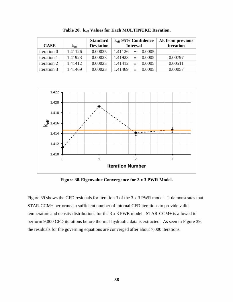
86
Table 20. keff Values for Each MULTINUKE Iteration.
CASE keff
Standard
Deviation
keff 95% Confidence
Interval
Δk from previous
iteration
iteration 0 1.41126 0.00025 1.41126 ± 0.0005 ----
iteration 1 1.41923 0.00023 1.41923 ± 0.0005 0.00797
iteration 2 1.41412 0.00023 1.41412 ± 0.0005 0.00511
iteration 3 1.41469 0.00023 1.41469 ± 0.0005 0.00057
Figure 38. Eigenvalue Convergence for 3 x 3 PWR Model.
Figure 39 shows the CFD residuals for iteration 3 of the 3 x 3 PWR model. It demonstrates that
STAR-CCM+ performed a sufficient number of internal CFD iterations to provide valid
temperature and density distributions for the 3 x 3 PWR model. STAR-CCM+ is allowed to
perform 9,000 CFD iterations before thermal-hydraulic data is extracted. As seen in Figure 39,
the residuals for the governing equations are converged after about 7,000 iterations.
1.410
1.412
1.414
1.416
1.418
1.420
1.422
0 1 2 3
k eff
Iteration Number

87
Figure 39. CFD Residuals Convergence for 3 x 3 PWR Model.
Figure 40 shows normalized axial power distributions for each MULTINUKE iteration of the
PWR lattice model. Axial power peaking converges to the red curve by iteration 3. More power
is generated in the lower half of the model due to significantly lower moderator temperature (and
thus higher density) in this region. The coolant temperature increases by almost 50 K in the first
MULTINUKE iteration, due to the model’s high power level and slow coolant velocity. This
causes the coolant density to be significantly less in the upper region of the model, shifting
thermal neutron flux and power to the lower region.

88
Figure 40. Converged Axial Power Peaking for 3 x 3 PWR Model.
Figure 41 shows the power density data, calculated using MCNP5, given to STAR-CCM+ for
the final MULTINUKE iteration. Fuel cells near the edge of the fuel pin are exposed to greater
thermal neutron flux compared to cells near the fuel center, due to self-shielding. The outer fuel
cells therefore have greater fission reaction rates and higher power densities, as shown in Figure
41. However, power densities shift to the lower half of the model in iteration 3.
0
25
50
75
100
125
150
175
200
225
250
275
300
325
350
0 0.2 0.4 0.6 0.8 1 1.2 1.4 1.6 1.8
Axi
al H
eigh
t (c
m)
Axial Peaking Factor
Iteration 0(isothermal calc)Iteration 1
Iteration 2
Iteration 3

89
Figure 41. Axial Power Density Distributions for Different Radial Distances from Fuel
Centerline in Fuel Element 2 (Iteration 3).
A contour plot of the radial power distribution at z = 117 cm (where power density is highest in
Figure 41) is shown by Figure 42. It confirms that power density, and thus fission reaction rates,
are greatest near the edge of each pin (as shown in Figure 41). The data for Figure 42 is from a
MCNP5 mesh tally, where a tally grid is superimposed over the actual problem geometry. The
grid used for the mesh tally in Figure 42 is of higher resolution than the computational mesh
used for the coupled MULTINUKE simulation, which is shown by the black lines. Hence, the
mesh tally contains more detailed radial power information than the MULTINUKE mesh in
Figure 41. The contour data is normalized tally data obtained directly from MCNP5.
r ≈ 0.14 cm to 0.40 cm r ≈ 0.44 cm
r ≈ 0.47 cm

90
In Figure 42, the maximum power density is approximately 0.0087 MeV/g/s (per starting
neutron). This is equivalent to 3.80x10⁸ W/m
3, which is only about 2 % greater than the
maximum power density calculated by MCNP5 with the coarser MULTINUKE mesh (3.73 x10⁸
W/m3 from Figure 41). Power density is greatest at the edges of the fuel regions closest to the
control rod guide tube, which is filled with water and thus creates a region of high thermal
neutron flux in the center of the model.
Figure 42. Radial Power Density Distribution at z = 117 cm (Iteration 3).

91
Figure 43 shows the axial distribution of fuel temperatures in element 2 for different radial
distances from the fuel centerline. As seen in Figure 43, fuel cells near the center of the pin have
higher temperatures. The maximum fuel temperature is about 922 K, occurring at z = 0.98 m.
Figure 43. Axial Fuel Temperature Distributions for Different Radial Locations in Element
2 (Iteration 3).
Figure 44 shows the axial distribution of the maximum fuel temperatures at each axial level,
comparing the first iteration to the third iteration. Figure 44 shows that the maximum fuel
temperature for the third iteration is greater than that of the first iteration (and occurs lower in the
model), which is due to the axial power distribution being compressed to the lower part of the
model. The temperature distributions for the fuel, clad, and water regions for the second
r ≈ 0.47 cm
r ≈ 0.44 cm
r ≈ 0.40 cm
r ≈ 0.31 cm
r ≈ 0.14 cm

92
iteration nearly match those from the third iteration, and are therefore omitted from the following
temperature plots.
Figure 44. Maximum Axial Temperatures for Fuel Region in Element 2.
Figure 45 shows the axial distribution of the maximum cladding temperatures at each axial level,
comparing the first iteration to the last iteration. Figure 45 shows that PCT for iteration 3 is
approximately 629.4 K, occurring at z = 1.6 m. The PCT for iteration 3 occurs lower in the
model than the PCT from iteration 1. PCT for iteration 3 is also slightly less (629.4 K compared
to 632 K for iteration 1), most likely due to PCT being located in the lower region of the model
where coolant temperatures are significantly less than they are in the upper region, thereby
enhancing the cooling of the cladding region.
0.0
0.5
1.0
1.5
2.0
2.5
3.0
3.5
550 600 650 700 750 800 850 900 950
Axi
al H
eig
ht
(m)
Temperature (K)
Iteration 1
Iteration 3
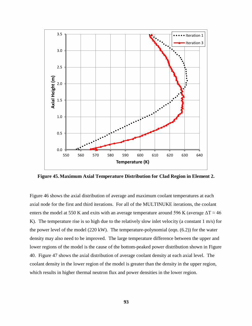
93
Figure 45. Maximum Axial Temperature Distribution for Clad Region in Element 2.
Figure 46 shows the axial distribution of average and maximum coolant temperatures at each
axial node for the first and third iterations. For all of the MULTINUKE iterations, the coolant
enters the model at 550 K and exits with an average temperature around 596 K (average ΔT ≈ 46
K). The temperature rise is so high due to the relatively slow inlet velocity (a constant 1 m/s) for
the power level of the model (220 kW). The temperature-polynomial (eqn. (6.2)) for the water
density may also need to be improved. The large temperature difference between the upper and
lower regions of the model is the cause of the bottom-peaked power distribution shown in Figure
40. Figure 47 shows the axial distribution of average coolant density at each axial level. The
coolant density in the lower region of the model is greater than the density in the upper region,
which results in higher thermal neutron flux and power densities in the lower region.
0.0
0.5
1.0
1.5
2.0
2.5
3.0
3.5
550 560 570 580 590 600 610 620 630 640
Axi
al H
eig
ht
(m)
Temperature (K)
Iteration 1
Iteration 3

94
Figure 46. Axial Temperature Distributions for Coolant in Element 2.
Figure 47. Axial Distribution of Average Coolant Density in Element 2 (Iteration 3).
0.0
0.5
1.0
1.5
2.0
2.5
3.0
3.5
550 555 560 565 570 575 580 585 590 595 600 605
Axi
al H
eig
ht
(m)
Temperature (K)
Iteration 1 - Average
Iteration 1 - Maximum
Iteration 3 - Average
Iteration 3 - Maximum
0.0
0.5
1.0
1.5
2.0
2.5
3.0
3.5
640 660 680 700 720 740 760 780
Axi
al H
eig
ht
(m)
Density (kg/m3)

95
Chapter 7. Summary
7.1. Conclusions
The MCNP5 Monte Carlo particle transport code has been coupled to the computational fluid
dynamics code, STAR-CCM+, to provide a high fidelity multi-physics simulation tool for
pressurized water nuclear reactors. The codes were executed separately and coupled externally
through a Perl script that automated the exchange of temperature, density, and volumetric
heating information between the codes using ASCII text data files.
The single PWR cell test case provided verification of the methodology used to couple the
neutronic and CFD codes. The MCNP5 cell model provided evidence of converged eigenvalue
and fission source distribution. Furthermore, the MCNP5 model had adequate tally statistics and
intuitively expected reactivity coefficients. The STAR-CCM+ cell model had appropriate
residuals convergence for the CFD simulations. A finer, unstructured, polyhedral mesh of the
PWR cell model was compared to the base hexahedral mesh results – showing acceptable axial
fuel temperature distribution agreement. Finally, the coupled MULTINUKE simulation
demonstrated realistic and intuitive power distributions, temperature distributions, coolant
densities, and fluid flow characteristics for a simple PWR model.
The shortened height of the first test model (20 cm PWR cell) did not allow for a very clear
demonstration of thermal-hydraulic feedback influencing the axial power distribution.
Considering the PWR cell model’s inlet velocity and total power level, the resulting distribution
of coolant density (lower near the exit and higher near the inlet) was not significant enough to
push power peaking to the lower region in such a short model, as it would be for a BWR (or the
3 x 3 PWR lattice model). However, the cell model results from Chapter 6 were successful in
demonstrating the effects that reduced coolant density and higher fuel temperatures have on
overall reactivity. In addition, the power distributions calculated by MCNP5 had a clear impact
on the temperature distributions in the fuel, clad, and coolant regions.

96
The simulation of the 3 x 3 PWR model expanded upon the results for the single 20 cm cell,
demonstrating clearer feedback effects between the CFD and neutronic solvers, due to the more
realistic size of the 3 x 3 model. Specifically, coolant temperatures increased more dramatically
along the height of the model, thereby lowering coolant density in the upper region of the core,
and resulting in a more bottom-peaked power distribution relative to the single PWR cell results.
Fuel and clad temperatures peaked lower in the 3 x 3 model as a result. In the absence of control
rods and axial variations of fuel and poison, the axial power peaking seen with this model is
probably excessive for a PWR – meaning the inlet velocity, power level, and moderator density
equation need some adjustments to obtain more realistic PWR behavior. The 3 x 3 PWR model
has a water hole in the middle of the model due to the water-filled guide tube. Therefore, fission
reaction rates (and power densities) were highest along the outer edge of the fuel pins nearest to
the center guide tube, since thermal neutron flux was highest near the center of the 3 x 3 PWR
model.
7.2. Further Work with MULTINUKE
The mesh for the 3 x 3 PWR model could be refined since it only has 89,856 CFD cells. In
creating the 3 x 3 model, the same axial mesh (104 nodes) from the 20 cm PWR cell was used to
avoid having the re-correlate the CFD mesh to the neutronic mesh. In addition, it preserved a
one-to-one relation between the fuel and moderator cells for both meshes, bypassing the need
add code to MULTINUKE to transfer data between two meshes of differing cell count and
volume. Most importantly, building upon the old mesh allowed the 3 x 3 PWR simulation to run
reasonably fast on a single quad-core machine. Eventually, the CFD mesh for the 3 x 3 model
should be refined to approximately 400-600 axial nodes. The radial mesh should also be refined
to better capture heat transfer and coolant flow behavior in the boundary layer. This is required
for more accurate thermal-hydraulic simulation of a 3 x 3 model that is 400 cm tall. Higher
fidelity turbulence models, such as the Reynolds Stress Transport model, would further increase
the accuracy of the 3 x 3 PWR simulation. Some code would need to be added to MULTINUKE
to transfer data between different MCNP5 and STAR-CCM+ meshes.

97
Beyond PWR assembly models, it is hoped that MULTINUKE may eventually be used for more
advanced, time-dependent applications. Specifically, further development of MULTINUKE
would include its implementation on massively parallel supercomputers. Calculation times for
the simple PWR models analyzed in this work were between 8 and 130 hours on just four cores
of a quad-processor machine. Massively parallel computing with MULTINUKE could analyze
large nuclear reactor models with more complicated neutronic–thermal-hydraulic feedback
effects, such as BWRs and fast reactors. For transient and accident analysis, STAR-CCM+
could be used in time-dependent mode, with MCNP5 providing updated power distributions at
appropriate time intervals. (MCNP5 has the capability for time-dependent, user-specified
sources and temperatures, but it has no direct transient or depletion capability.) Such advanced,
high fidelity, multi-physics reactor simulations can assist in furthering the state-of-the-art
through innovative validation of reactor safety and economic viability.

98
References
[1] F. B. Brown, J. T. Goorley, and J. E. Sweezy, "MCNP5 Parallel Processing
Workshop," Proceedings of ANS Mathematics & Computation Topical Meeting,
Gatlinburg, Tennessee, April 11 (2003).
[2] P. Finck, D. Keyes, and R. Stevens, “Workshop on Simulation and Modeling for
Advanced Nuclear Energy Systems,” Washington, D.C., August 15-17 (2006).
Available at http://www.er.doe.gov/ascr/Misc/gnep06-final.pdf.
[3] US Department of Energy Webpage, “Modeling & Simulation for Nuclear Reactors,”
http://www.energy.gov/hubs/modeling_simulation_nuclear_reactors.htm, May 28
(2010). Accessed June 28, 2010.
[4] X-5 Monte Carlo Team, “MCNP – A General Monte Carlo N-Particle Transport
Code, Version 5,” Los Alamos, New Mexico (2008).
[5] M. M. El-Wakil, Nuclear Heat Transport, The American Nuclear Society, La Grange
Park, Illinois (1993).
[6] J. J. Duderstadt and L. J. Hamilton, Nuclear Reactor Analysis, John Wiley & Sons,
New York, New York (1976).
[7] W. M. Stacey, Nuclear Reactor Physics, Wiley-VCH, Weinheim, Germany (2007).
[8] J. R. Lamarsh and A. J. Baratta, Introduction to Nuclear Engineering, Prentice Hall,
Upper Saddle River, New Jersey (2001).
[9] T. M. Sutton, T. J. Donovan, T. H. Trumbull, P. S. Dobreff, E. Caro, D. P.
Griesheimer, L. J. Tyburski, D. C. Carpenter, and H. Joo, “The MC21 Monte Carlo
Transport Code,” Proceedings of Joint International Topical Meeting on Mathematics
& Computation and Supercomputing in Nuclear Applications, Monterey, California,
April 15-19 (2007).

99
[10] R. E. Macfarlane et al., “NJOY99.0: Code System for Producing Pointwise and
Multigroup Neutron and Photon Cross Sections from ENDF/B Data,” Los Alamos,
New Mexico (2000). Basic NJOY information available at http://t2.lanl.gov/njoy/.
[11] V. Seker, J. W. Thomas, and T. J. Downar, “Reactor Physics Simulations With
Coupled Monte Carlo Calculation and Computational Fluid Dynamics,” Proceedings
of International Conference on Emerging Nuclear Energy Systems, Istanbul, Turkey,
June 3-8 (2007).
[12] S. Kimhy and A. Galperin, “Simple Model of Thermal-Hydraulic Feedback for
Neutronic Analysis of PWR Cores,” Annals of Nuclear Energy, Vol. 15, No. 2, pp.
95-100 (1988).
[13] D. P. Weber et al., “High Fidelity LWR Analysis with the Numerical Nuclear
Reactor,” Nuclear Science and Engineering, Vol. 155, pp. 1-14 (2007).
[14] J. Hu and Rizwan-uddin, “Coupled Neutronics and Thermal-Hydraulics Using MCNP
and FLUENT,” Transactions of the American Nuclear Society, Vol. 98, pp. 606-608
(2008).
[15] CD-adapco Webpage. “Product Overview,” http://www.cd-adapco.com/products/,
CD-adapco, (2010). Accessed October 15, 2010.
[16] X-5 Monte Carlo Team, “MCNP5 1.50 Release Notes,” Los Alamos, New Mexico
(2008).
[17] T. J. Downar, A. Siegel, C. Unal, et al. “Science Based Nuclear Energy Systems
Enabled by Advanced Modeling and Simulation at the Extreme Scale,” Crystal City,
Virginia, May 11-12 (2009).
[18] The RELAP5-3D© Code Development Team, “RELAP5-3D
© Code Manual
Volume 1: Code Structure, System Models, and Solution Methods,” Idaho Falls,
Idaho (2005).

100
[19] F. B. Brown, “The makxsf Code with Doppler Broadening,” Los Alamos, New
Mexico (2008).
[20] G. K. Batchelor, An Introduction to Fluid Dynamics, Cambridge University Press,
New York, New York (2000).
[21] N. E. Todreas and M. S. Kazimi, Nuclear Systems I, Taylor & Francis, New York,
New York (1993).
[22] CD-adapco, “User Guide: STAR-CCM+ Version 2.10.017,” CD-adapco (2007).
[23] D. P. Weber, T. Sofu, T. H. Chun, H. G. Joo, J. W. Thomas, Z. Zhong, T. J. Downar,
“Development of Comprehensive Modeling Capability Based on Rigorous Treatment
of Multi-Physics Phenomena Influencing Reactor Core Design,” Proceedings of
International Congress on Advances in Nuclear Power Plants, Pittsburgh,
Pennsylvania, June 13-17 (2004).
[24] L. Snoj and M. Ravnik, "Calculation of Power Density with MCNP in TRIGA
Reactor," Proceedings of International Conference on Nuclear Energy for New
Europe, Portoroz, Slovenia, September 18-21 (2006).
[25] B. El Bakkari, T. El Bardouni, O. Merroun, C. El Younoussi, Y. Boulaich, and E.
Chakir, “Development of an MCNP Tally Based Burnup Code and Validation
Through PWR Benchmark Exercises,” Annals of Nuclear Energy, Vol. 36, pp. 626-
633 (2009).
[26] Argonne National Laboratory Webpage for the International Nuclear Safety Center,
“Thermal Conductivity and Thermal Diffusivity of Solid UO2,”
http://www.insc.anl.gov/matprop/uo2/cond/solid/thcsuo2.pdf, July (1999). Accessed
August 8, 2010.

101
[27] Argonne National Laboratory Webpage for the International Nuclear Safety Center,
“Zircaloy Thermal Conductivity,”
http://www.insc.anl.gov/matprop/zircaloy/zirck.pdf, July (1999). Accessed May 4,
2010.
[28] Argonne National Laboratory Webpage for the International Nuclear Safety Center,
“Zircaloy Heat Capacity,”
http://www.insc.anl.gov/matprop/zircaloy/zirccp/fmt_orig.pdf, October (1997).
Accessed May 4, 2010.
[29] F. B. Brown, W. Martine, J. Leppanen, W. Haeck, and B. Cochet, "Reactor Physics
Analysis with Monte Carlo," Proceedings of ANS PHYSOR-2010 Conference
Workshop, Pittsburgh, Pennsylvania, May 9 (2010).

102
APPENDIX A. Base Input Files for PWR Cell Model
Complete input files for the PWR cell model can be found in multinuke.zip.
A.1 MCNP5 Input File Excerpts pin20cm : 5.0% enriched UO2 pin in H20 block - with grids
c
c ****************************
c *** cell definitions ***
c ****************************
c
c cell# material# density surfaces tmpTemperature importance
c
c fuel cells 1-3328
1 f_0001 6.874E-02 -1 12 -13 21 -22 99 -100 tmp=ft0001 imp:n=1 $ fuel pin grid block axial seg 1
2 f_0002 6.874E-02 -1 13 -14 21 -22 99 -100 tmp=ft0002 imp:n=1 $ fuel pin grid block axial seg 1
3 f_0003 6.874E-02 -1 14 -15 21 -22 99 -100 tmp=ft0003 imp:n=1 $ fuel pin grid block axial seg 1
4 f_0004 6.874E-02 -1 15 -16 21 -22 99 -100 tmp=ft0004 imp:n=1 $ fuel pin grid block axial seg 1
5 f_0005 6.874E-02 -1 11 -12 22 -23 99 -100 tmp=ft0005 imp:n=1 $ fuel pin grid block axial seg 1
6 f_0006 6.874E-02 -1 12 -13 22 -23 99 -100 tmp=ft0006 imp:n=1 $ fuel pin grid block axial seg 1
7 f_0007 6.874E-02 -1 13 -14 22 -23 99 -100 tmp=ft0007 imp:n=1 $ fuel pin grid block axial seg 1
8 f_0008 6.874E-02 -1 14 -15 22 -23 99 -100 tmp=ft0008 imp:n=1 $ fuel pin grid block axial seg 1
9 f_0009 6.874E-02 -1 15 -16 22 -23 99 -100 tmp=ft0009 imp:n=1 $ fuel pin grid block axial seg 1
10 f_0010 6.874E-02 -1 16 -17 22 -23 99 -100 tmp=ft0010 imp:n=1 $ fuel pin grid block axial seg 1
11 f_0011 6.874E-02 -1 11 -12 23 -24 99 -100 tmp=ft0011 imp:n=1 $ fuel pin grid block axial seg 1
12 f_0012 6.874E-02 -1 12 -13 23 -24 99 -100 tmp=ft0012 imp:n=1 $ fuel pin grid block axial seg 1
13 f_0013 6.874E-02 -1 13 -14 23 -24 99 -100 tmp=ft0013 imp:n=1 $ fuel pin grid block axial seg 1
14 f_0014 6.874E-02 -1 14 -15 23 -24 99 -100 tmp=ft0014 imp:n=1 $ fuel pin grid block axial seg 1
15 f_0015 6.874E-02 -1 15 -16 23 -24 99 -100 tmp=ft0015 imp:n=1 $ fuel pin grid block axial seg 1
16 f_0016 6.874E-02 -1 16 -17 23 -24 99 -100 tmp=ft0016 imp:n=1 $ fuel pin grid block axial seg 1
17 f_0017 6.874E-02 -1 11 -12 24 -25 99 -100 tmp=ft0017 imp:n=1 $ fuel pin grid block axial seg 1
18 f_0018 6.874E-02 -1 12 -13 24 -25 99 -100 tmp=ft0018 imp:n=1 $ fuel pin grid block axial seg 1
19 f_0019 6.874E-02 -1 13 -14 24 -25 99 -100 tmp=ft0019 imp:n=1 $ fuel pin grid block axial seg 1
20 f_0020 6.874E-02 -1 14 -15 24 -25 99 -100 tmp=ft0020 imp:n=1 $ fuel pin grid block axial seg 1
21 f_0021 6.874E-02 -1 15 -16 24 -25 99 -100 tmp=ft0021 imp:n=1 $ fuel pin grid block axial seg 1
22 f_0022 6.874E-02 -1 16 -17 24 -25 99 -100 tmp=ft0022 imp:n=1 $ fuel pin grid block axial seg 1
23 f_0023 6.874E-02 -1 11 -12 25 -26 99 -100 tmp=ft0023 imp:n=1 $ fuel pin grid block axial seg 1
24 f_0024 6.874E-02 -1 12 -13 25 -26 99 -100 tmp=ft0024 imp:n=1 $ fuel pin grid block axial seg 1
25 f_0025 6.874E-02 -1 13 -14 25 -26 99 -100 tmp=ft0025 imp:n=1 $ fuel pin grid block axial seg 1
26 f_0026 6.874E-02 -1 14 -15 25 -26 99 -100 tmp=ft0026 imp:n=1 $ fuel pin grid block axial seg 1
27 f_0027 6.874E-02 -1 15 -16 25 -26 99 -100 tmp=ft0027 imp:n=1 $ fuel pin grid block axial seg 1
28 f_0028 6.874E-02 -1 16 -17 25 -26 99 -100 tmp=ft0028 imp:n=1 $ fuel pin grid block axial seg 1
29 f_0029 6.874E-02 -1 12 -13 26 -27 99 -100 tmp=ft0029 imp:n=1 $ fuel pin grid block axial seg 1
30 f_0030 6.874E-02 -1 13 -14 26 -27 99 -100 tmp=ft0030 imp:n=1 $ fuel pin grid block axial seg 1
31 f_0031 6.874E-02 -1 14 -15 26 -27 99 -100 tmp=ft0031 imp:n=1 $ fuel pin grid block axial seg 1
32 f_0032 6.874E-02 -1 15 -16 26 -27 99 -100 tmp=ft0032 imp:n=1 $ fuel pin grid block axial seg 1
33 f_0033 6.874E-02 -1 12 -13 21 -22 100 -101 tmp=ft0033 imp:n=1 $ fuel pin grid block axial seg 2
34 f_0034 6.874E-02 -1 13 -14 21 -22 100 -101 tmp=ft0034 imp:n=1 $ fuel pin grid block axial seg 2
35 f_0035 6.874E-02 -1 14 -15 21 -22 100 -101 tmp=ft0035 imp:n=1 $ fuel pin grid block axial seg 2
36 f_0036 6.874E-02 -1 15 -16 21 -22 100 -101 tmp=ft0036 imp:n=1 $ fuel pin grid block axial seg 2
37 f_0037 6.874E-02 -1 11 -12 22 -23 100 -101 tmp=ft0037 imp:n=1 $ fuel pin grid block axial seg 2
38 f_0038 6.874E-02 -1 12 -13 22 -23 100 -101 tmp=ft0038 imp:n=1 $ fuel pin grid block axial seg 2
39 f_0039 6.874E-02 -1 13 -14 22 -23 100 -101 tmp=ft0039 imp:n=1 $ fuel pin grid block axial seg 2
40 f_0040 6.874E-02 -1 14 -15 22 -23 100 -101 tmp=ft0040 imp:n=1 $ fuel pin grid block axial seg 2
41 f_0041 6.874E-02 -1 15 -16 22 -23 100 -101 tmp=ft0041 imp:n=1 $ fuel pin grid block axial seg 2
42 f_0042 6.874E-02 -1 16 -17 22 -23 100 -101 tmp=ft0042 imp:n=1 $ fuel pin grid block axial seg 2
43 f_0043 6.874E-02 -1 11 -12 23 -24 100 -101 tmp=ft0043 imp:n=1 $ fuel pin grid block axial seg 2
44 f_0044 6.874E-02 -1 12 -13 23 -24 100 -101 tmp=ft0044 imp:n=1 $ fuel pin grid block axial seg 2
45 f_0045 6.874E-02 -1 13 -14 23 -24 100 -101 tmp=ft0045 imp:n=1 $ fuel pin grid block axial seg 2
46 f_0046 6.874E-02 -1 14 -15 23 -24 100 -101 tmp=ft0046 imp:n=1 $ fuel pin grid block axial seg 2
47 f_0047 6.874E-02 -1 15 -16 23 -24 100 -101 tmp=ft0047 imp:n=1 $ fuel pin grid block axial seg 2
48 f_0048 6.874E-02 -1 16 -17 23 -24 100 -101 tmp=ft0048 imp:n=1 $ fuel pin grid block axial seg 2
49 f_0049 6.874E-02 -1 11 -12 24 -25 100 -101 tmp=ft0049 imp:n=1 $ fuel pin grid block axial seg 2
50 f_0050 6.874E-02 -1 12 -13 24 -25 100 -101 tmp=ft0050 imp:n=1 $ fuel pin grid block axial seg 2
51 f_0051 6.874E-02 -1 13 -14 24 -25 100 -101 tmp=ft0051 imp:n=1 $ fuel pin grid block axial seg 2
52 f_0052 6.874E-02 -1 14 -15 24 -25 100 -101 tmp=ft0052 imp:n=1 $ fuel pin grid block axial seg 2
53 f_0053 6.874E-02 -1 15 -16 24 -25 100 -101 tmp=ft0053 imp:n=1 $ fuel pin grid block axial seg 2
54 f_0054 6.874E-02 -1 16 -17 24 -25 100 -101 tmp=ft0054 imp:n=1 $ fuel pin grid block axial seg 2
55 f_0055 6.874E-02 -1 11 -12 25 -26 100 -101 tmp=ft0055 imp:n=1 $ fuel pin grid block axial seg 2
56 f_0056 6.874E-02 -1 12 -13 25 -26 100 -101 tmp=ft0056 imp:n=1 $ fuel pin grid block axial seg 2
57 f_0057 6.874E-02 -1 13 -14 25 -26 100 -101 tmp=ft0057 imp:n=1 $ fuel pin grid block axial seg 2
58 f_0058 6.874E-02 -1 14 -15 25 -26 100 -101 tmp=ft0058 imp:n=1 $ fuel pin grid block axial seg 2
59 f_0059 6.874E-02 -1 15 -16 25 -26 100 -101 tmp=ft0059 imp:n=1 $ fuel pin grid block axial seg 2

103
60 f_0060 6.874E-02 -1 16 -17 25 -26 100 -101 tmp=ft0060 imp:n=1 $ fuel pin grid block axial seg 2
61 f_0061 6.874E-02 -1 12 -13 26 -27 100 -101 tmp=ft0061 imp:n=1 $ fuel pin grid block axial seg 2
62 f_0062 6.874E-02 -1 13 -14 26 -27 100 -101 tmp=ft0062 imp:n=1 $ fuel pin grid block axial seg 2
63 f_0063 6.874E-02 -1 14 -15 26 -27 100 -101 tmp=ft0063 imp:n=1 $ fuel pin grid block axial seg 2
64 f_0064 6.874E-02 -1 15 -16 26 -27 100 -101 tmp=ft0064 imp:n=1 $ fuel pin grid block axial seg 2
65 f_0065 6.874E-02 -1 12 -13 21 -22 101 -102 tmp=ft0065 imp:n=1 $ fuel pin grid block axial seg 3
66 f_0066 6.874E-02 -1 13 -14 21 -22 101 -102 tmp=ft0066 imp:n=1 $ fuel pin grid block axial seg 3
67 f_0067 6.874E-02 -1 14 -15 21 -22 101 -102 tmp=ft0067 imp:n=1 $ fuel pin grid block axial seg 3
68 f_0068 6.874E-02 -1 15 -16 21 -22 101 -102 tmp=ft0068 imp:n=1 $ fuel pin grid block axial seg 3
69 f_0069 6.874E-02 -1 11 -12 22 -23 101 -102 tmp=ft0069 imp:n=1 $ fuel pin grid block axial seg 3
70 f_0070 6.874E-02 -1 12 -13 22 -23 101 -102 tmp=ft0070 imp:n=1 $ fuel pin grid block axial seg 3
71 f_0071 6.874E-02 -1 13 -14 22 -23 101 -102 tmp=ft0071 imp:n=1 $ fuel pin grid block axial seg 3
72 f_0072 6.874E-02 -1 14 -15 22 -23 101 -102 tmp=ft0072 imp:n=1 $ fuel pin grid block axial seg 3
73 f_0073 6.874E-02 -1 15 -16 22 -23 101 -102 tmp=ft0073 imp:n=1 $ fuel pin grid block axial seg 3
74 f_0074 6.874E-02 -1 16 -17 22 -23 101 -102 tmp=ft0074 imp:n=1 $ fuel pin grid block axial seg 3
75 f_0075 6.874E-02 -1 11 -12 23 -24 101 -102 tmp=ft0075 imp:n=1 $ fuel pin grid block axial seg 3
76 f_0076 6.874E-02 -1 12 -13 23 -24 101 -102 tmp=ft0076 imp:n=1 $ fuel pin grid block axial seg 3
77 f_0077 6.874E-02 -1 13 -14 23 -24 101 -102 tmp=ft0077 imp:n=1 $ fuel pin grid block axial seg 3
78 f_0078 6.874E-02 -1 14 -15 23 -24 101 -102 tmp=ft0078 imp:n=1 $ fuel pin grid block axial seg 3
79 f_0079 6.874E-02 -1 15 -16 23 -24 101 -102 tmp=ft0079 imp:n=1 $ fuel pin grid block axial seg 3
80 f_0080 6.874E-02 -1 16 -17 23 -24 101 -102 tmp=ft0080 imp:n=1 $ fuel pin grid block axial seg 3
81 f_0081 6.874E-02 -1 11 -12 24 -25 101 -102 tmp=ft0081 imp:n=1 $ fuel pin grid block axial seg 3
82 f_0082 6.874E-02 -1 12 -13 24 -25 101 -102 tmp=ft0082 imp:n=1 $ fuel pin grid block axial seg 3
83 f_0083 6.874E-02 -1 13 -14 24 -25 101 -102 tmp=ft0083 imp:n=1 $ fuel pin grid block axial seg 3
84 f_0084 6.874E-02 -1 14 -15 24 -25 101 -102 tmp=ft0084 imp:n=1 $ fuel pin grid block axial seg 3
85 f_0085 6.874E-02 -1 15 -16 24 -25 101 -102 tmp=ft0085 imp:n=1 $ fuel pin grid block axial seg 3
86 f_0086 6.874E-02 -1 16 -17 24 -25 101 -102 tmp=ft0086 imp:n=1 $ fuel pin grid block axial seg 3
87 f_0087 6.874E-02 -1 11 -12 25 -26 101 -102 tmp=ft0087 imp:n=1 $ fuel pin grid block axial seg 3
88 f_0088 6.874E-02 -1 12 -13 25 -26 101 -102 tmp=ft0088 imp:n=1 $ fuel pin grid block axial seg 3
89 f_0089 6.874E-02 -1 13 -14 25 -26 101 -102 tmp=ft0089 imp:n=1 $ fuel pin grid block axial seg 3
90 f_0090 6.874E-02 -1 14 -15 25 -26 101 -102 tmp=ft0090 imp:n=1 $ fuel pin grid block axial seg 3
91 f_0091 6.874E-02 -1 15 -16 25 -26 101 -102 tmp=ft0091 imp:n=1 $ fuel pin grid block axial seg 3
92 f_0092 6.874E-02 -1 16 -17 25 -26 101 -102 tmp=ft0092 imp:n=1 $ fuel pin grid block axial seg 3
93 f_0093 6.874E-02 -1 12 -13 26 -27 101 -102 tmp=ft0093 imp:n=1 $ fuel pin grid block axial seg 3
94 f_0094 6.874E-02 -1 13 -14 26 -27 101 -102 tmp=ft0094 imp:n=1 $ fuel pin grid block axial seg 3
95 f_0095 6.874E-02 -1 14 -15 26 -27 101 -102 tmp=ft0095 imp:n=1 $ fuel pin grid block axial seg 3
96 f_0096 6.874E-02 -1 15 -16 26 -27 101 -102 tmp=ft0096 imp:n=1 $ fuel pin grid block axial seg 3
97 f_0097 6.874E-02 -1 12 -13 21 -22 102 -103 tmp=ft0097 imp:n=1 $ fuel pin grid block axial seg 4
98 f_0098 6.874E-02 -1 13 -14 21 -22 102 -103 tmp=ft0098 imp:n=1 $ fuel pin grid block axial seg 4
99 f_0099 6.874E-02 -1 14 -15 21 -22 102 -103 tmp=ft0099 imp:n=1 $ fuel pin grid block axial seg 4
100 f_0100 6.874E-02 -1 15 -16 21 -22 102 -103 tmp=ft0100 imp:n=1 $ fuel pin grid block axial seg 4
101 f_0101 6.874E-02 -1 11 -12 22 -23 102 -103 tmp=ft0101 imp:n=1 $ fuel pin grid block axial seg 4
102 f_0102 6.874E-02 -1 12 -13 22 -23 102 -103 tmp=ft0102 imp:n=1 $ fuel pin grid block axial seg 4
103 f_0103 6.874E-02 -1 13 -14 22 -23 102 -103 tmp=ft0103 imp:n=1 $ fuel pin grid block axial seg 4
104 f_0104 6.874E-02 -1 14 -15 22 -23 102 -103 tmp=ft0104 imp:n=1 $ fuel pin grid block axial seg 4
105 f_0105 6.874E-02 -1 15 -16 22 -23 102 -103 tmp=ft0105 imp:n=1 $ fuel pin grid block axial seg 4
106 f_0106 6.874E-02 -1 16 -17 22 -23 102 -103 tmp=ft0106 imp:n=1 $ fuel pin grid block axial seg 4
107 f_0107 6.874E-02 -1 11 -12 23 -24 102 -103 tmp=ft0107 imp:n=1 $ fuel pin grid block axial seg 4
108 f_0108 6.874E-02 -1 12 -13 23 -24 102 -103 tmp=ft0108 imp:n=1 $ fuel pin grid block axial seg 4
109 f_0109 6.874E-02 -1 13 -14 23 -24 102 -103 tmp=ft0109 imp:n=1 $ fuel pin grid block axial seg 4
110 f_0110 6.874E-02 -1 14 -15 23 -24 102 -103 tmp=ft0110 imp:n=1 $ fuel pin grid block axial seg 4
111 f_0111 6.874E-02 -1 15 -16 23 -24 102 -103 tmp=ft0111 imp:n=1 $ fuel pin grid block axial seg 4
.
.
(Fuel cell cards continue)
.
. c (WATER CELLS)
4001 w_4001 wden_4001 2 10 -11 20 -21 99 -100 tmp=wt4001 imp:n=1 $ water grid block axial seg 1
4002 w_4002 wden_4002 2 11 -12 20 -21 99 -100 tmp=wt4002 imp:n=1 $ water grid block axial seg 1
4003 w_4003 wden_4003 2 12 -13 20 -21 99 -100 tmp=wt4003 imp:n=1 $ water grid block axial seg 1
4004 w_4004 wden_4004 2 13 -14 20 -21 99 -100 tmp=wt4004 imp:n=1 $ water grid block axial seg 1
4005 w_4005 wden_4005 2 14 -15 20 -21 99 -100 tmp=wt4005 imp:n=1 $ water grid block axial seg 1
4006 w_4006 wden_4006 2 15 -16 20 -21 99 -100 tmp=wt4006 imp:n=1 $ water grid block axial seg 1
4007 w_4007 wden_4007 2 16 -17 20 -21 99 -100 tmp=wt4007 imp:n=1 $ water grid block axial seg 1
4008 w_4008 wden_4008 2 17 -18 20 -21 99 -100 tmp=wt4008 imp:n=1 $ water grid block axial seg 1
4009 w_4009 wden_4009 2 10 -11 21 -22 99 -100 tmp=wt4009 imp:n=1 $ water grid block axial seg 1
4010 w_4010 wden_4010 2 11 -12 21 -22 99 -100 tmp=wt4010 imp:n=1 $ water grid block axial seg 1
4011 w_4011 wden_4011 2 12 -13 21 -22 99 -100 tmp=wt4011 imp:n=1 $ water grid block axial seg 1
4012 w_4012 wden_4012 2 15 -16 21 -22 99 -100 tmp=wt4012 imp:n=1 $ water grid block axial seg 1
4013 w_4013 wden_4013 2 16 -17 21 -22 99 -100 tmp=wt4013 imp:n=1 $ water grid block axial seg 1
4014 w_4014 wden_4014 2 17 -18 21 -22 99 -100 tmp=wt4014 imp:n=1 $ water grid block axial seg 1
4015 w_4015 wden_4015 2 10 -11 22 -23 99 -100 tmp=wt4015 imp:n=1 $ water grid block axial seg 1

104
4016 w_4016 wden_4016 2 11 -12 22 -23 99 -100 tmp=wt4016 imp:n=1 $ water grid block axial seg 1
4017 w_4017 wden_4017 2 16 -17 22 -23 99 -100 tmp=wt4017 imp:n=1 $ water grid block axial seg 1
4018 w_4018 wden_4018 2 17 -18 22 -23 99 -100 tmp=wt4018 imp:n=1 $ water grid block axial seg 1
4019 w_4019 wden_4019 2 10 -11 23 -24 99 -100 tmp=wt4019 imp:n=1 $ water grid block axial seg 1
4020 w_4020 wden_4020 2 17 -18 23 -24 99 -100 tmp=wt4020 imp:n=1 $ water grid block axial seg 1
4021 w_4021 wden_4021 2 10 -11 24 -25 99 -100 tmp=wt4021 imp:n=1 $ water grid block axial seg 1
4022 w_4022 wden_4022 2 17 -18 24 -25 99 -100 tmp=wt4022 imp:n=1 $ water grid block axial seg 1
4023 w_4023 wden_4023 2 10 -11 25 -26 99 -100 tmp=wt4023 imp:n=1 $ water grid block axial seg 1
4024 w_4024 wden_4024 2 11 -12 25 -26 99 -100 tmp=wt4024 imp:n=1 $ water grid block axial seg 1
4025 w_4025 wden_4025 2 16 -17 25 -26 99 -100 tmp=wt4025 imp:n=1 $ water grid block axial seg 1
4026 w_4026 wden_4026 2 17 -18 25 -26 99 -100 tmp=wt4026 imp:n=1 $ water grid block axial seg 1
4027 w_4027 wden_4027 2 10 -11 26 -27 99 -100 tmp=wt4027 imp:n=1 $ water grid block axial seg 1
4028 w_4028 wden_4028 2 11 -12 26 -27 99 -100 tmp=wt4028 imp:n=1 $ water grid block axial seg 1
4029 w_4029 wden_4029 2 12 -13 26 -27 99 -100 tmp=wt4029 imp:n=1 $ water grid block axial seg 1
4030 w_4030 wden_4030 2 15 -16 26 -27 99 -100 tmp=wt4030 imp:n=1 $ water grid block axial seg 1
4031 w_4031 wden_4031 2 16 -17 26 -27 99 -100 tmp=wt4031 imp:n=1 $ water grid block axial seg 1
4032 w_4032 wden_4032 2 17 -18 26 -27 99 -100 tmp=wt4032 imp:n=1 $ water grid block axial seg 1
4033 w_4033 wden_4033 2 10 -11 27 -28 99 -100 tmp=wt4033 imp:n=1 $ water grid block axial seg 1
4034 w_4034 wden_4034 2 11 -12 27 -28 99 -100 tmp=wt4034 imp:n=1 $ water grid block axial seg 1
4035 w_4035 wden_4035 2 12 -13 27 -28 99 -100 tmp=wt4035 imp:n=1 $ water grid block axial seg 1
4036 w_4036 wden_4036 2 13 -14 27 -28 99 -100 tmp=wt4036 imp:n=1 $ water grid block axial seg 1
4037 w_4037 wden_4037 2 14 -15 27 -28 99 -100 tmp=wt4037 imp:n=1 $ water grid block axial seg 1
4038 w_4038 wden_4038 2 15 -16 27 -28 99 -100 tmp=wt4038 imp:n=1 $ water grid block axial seg 1
4039 w_4039 wden_4039 2 16 -17 27 -28 99 -100 tmp=wt4039 imp:n=1 $ water grid block axial seg 1
4040 w_4040 wden_4040 2 17 -18 27 -28 99 -100 tmp=wt4040 imp:n=1 $ water grid block axial seg 1
4041 w_4041 wden_4041 2 10 -11 20 -21 100 -101 tmp=wt4041 imp:n=1 $ water grid block axial seg 2
4042 w_4042 wden_4042 2 11 -12 20 -21 100 -101 tmp=wt4042 imp:n=1 $ water grid block axial seg 2
4043 w_4043 wden_4043 2 12 -13 20 -21 100 -101 tmp=wt4043 imp:n=1 $ water grid block axial seg 2
4044 w_4044 wden_4044 2 13 -14 20 -21 100 -101 tmp=wt4044 imp:n=1 $ water grid block axial seg 2
4045 w_4045 wden_4045 2 14 -15 20 -21 100 -101 tmp=wt4045 imp:n=1 $ water grid block axial seg 2
4046 w_4046 wden_4046 2 15 -16 20 -21 100 -101 tmp=wt4046 imp:n=1 $ water grid block axial seg 2
4047 w_4047 wden_4047 2 16 -17 20 -21 100 -101 tmp=wt4047 imp:n=1 $ water grid block axial seg 2
4048 w_4048 wden_4048 2 17 -18 20 -21 100 -101 tmp=wt4048 imp:n=1 $ water grid block axial seg 2
4049 w_4049 wden_4049 2 10 -11 21 -22 100 -101 tmp=wt4049 imp:n=1 $ water grid block axial seg 2
4050 w_4050 wden_4050 2 11 -12 21 -22 100 -101 tmp=wt4050 imp:n=1 $ water grid block axial seg 2
4051 w_4051 wden_4051 2 12 -13 21 -22 100 -101 tmp=wt4051 imp:n=1 $ water grid block axial seg 2
4052 w_4052 wden_4052 2 15 -16 21 -22 100 -101 tmp=wt4052 imp:n=1 $ water grid block axial seg 2
4053 w_4053 wden_4053 2 16 -17 21 -22 100 -101 tmp=wt4053 imp:n=1 $ water grid block axial seg 2
4054 w_4054 wden_4054 2 17 -18 21 -22 100 -101 tmp=wt4054 imp:n=1 $ water grid block axial seg 2
4055 w_4055 wden_4055 2 10 -11 22 -23 100 -101 tmp=wt4055 imp:n=1 $ water grid block axial seg 2
4056 w_4056 wden_4056 2 11 -12 22 -23 100 -101 tmp=wt4056 imp:n=1 $ water grid block axial seg 2
4057 w_4057 wden_4057 2 16 -17 22 -23 100 -101 tmp=wt4057 imp:n=1 $ water grid block axial seg 2
4058 w_4058 wden_4058 2 17 -18 22 -23 100 -101 tmp=wt4058 imp:n=1 $ water grid block axial seg 2
4059 w_4059 wden_4059 2 10 -11 23 -24 100 -101 tmp=wt4059 imp:n=1 $ water grid block axial seg 2
4060 w_4060 wden_4060 2 17 -18 23 -24 100 -101 tmp=wt4060 imp:n=1 $ water grid block axial seg 2
4061 w_4061 wden_4061 2 10 -11 24 -25 100 -101 tmp=wt4061 imp:n=1 $ water grid block axial seg 2
4062 w_4062 wden_4062 2 17 -18 24 -25 100 -101 tmp=wt4062 imp:n=1 $ water grid block axial seg 2
4063 w_4063 wden_4063 2 10 -11 25 -26 100 -101 tmp=wt4063 imp:n=1 $ water grid block axial seg 2
4064 w_4064 wden_4064 2 11 -12 25 -26 100 -101 tmp=wt4064 imp:n=1 $ water grid block axial seg 2
4065 w_4065 wden_4065 2 16 -17 25 -26 100 -101 tmp=wt4065 imp:n=1 $ water grid block axial seg 2
4066 w_4066 wden_4066 2 17 -18 25 -26 100 -101 tmp=wt4066 imp:n=1 $ water grid block axial seg 2
4067 w_4067 wden_4067 2 10 -11 26 -27 100 -101 tmp=wt4067 imp:n=1 $ water grid block axial seg 2
4068 w_4068 wden_4068 2 11 -12 26 -27 100 -101 tmp=wt4068 imp:n=1 $ water grid block axial seg 2
4069 w_4069 wden_4069 2 12 -13 26 -27 100 -101 tmp=wt4069 imp:n=1 $ water grid block axial seg 2
4070 w_4070 wden_4070 2 15 -16 26 -27 100 -101 tmp=wt4070 imp:n=1 $ water grid block axial seg 2
4071 w_4071 wden_4071 2 16 -17 26 -27 100 -101 tmp=wt4071 imp:n=1 $ water grid block axial seg 2
4072 w_4072 wden_4072 2 17 -18 26 -27 100 -101 tmp=wt4072 imp:n=1 $ water grid block axial seg 2
4073 w_4073 wden_4073 2 10 -11 27 -28 100 -101 tmp=wt4073 imp:n=1 $ water grid block axial seg 2
4074 w_4074 wden_4074 2 11 -12 27 -28 100 -101 tmp=wt4074 imp:n=1 $ water grid block axial seg 2
4075 w_4075 wden_4075 2 12 -13 27 -28 100 -101 tmp=wt4075 imp:n=1 $ water grid block axial seg 2
4076 w_4076 wden_4076 2 13 -14 27 -28 100 -101 tmp=wt4076 imp:n=1 $ water grid block axial seg 2
4077 w_4077 wden_4077 2 14 -15 27 -28 100 -101 tmp=wt4077 imp:n=1 $ water grid block axial seg 2
4078 w_4078 wden_4078 2 15 -16 27 -28 100 -101 tmp=wt4078 imp:n=1 $ water grid block axial seg 2
4079 w_4079 wden_4079 2 16 -17 27 -28 100 -101 tmp=wt4079 imp:n=1 $ water grid block axial seg 2
4080 w_4080 wden_4080 2 17 -18 27 -28 100 -101 tmp=wt4080 imp:n=1 $ water grid block axial seg 2
4081 w_4081 wden_4081 2 10 -11 20 -21 101 -102 tmp=wt4081 imp:n=1 $ water grid block axial seg 3
4082 w_4082 wden_4082 2 11 -12 20 -21 101 -102 tmp=wt4082 imp:n=1 $ water grid block axial seg 3
4083 w_4083 wden_4083 2 12 -13 20 -21 101 -102 tmp=wt4083 imp:n=1 $ water grid block axial seg 3
4084 w_4084 wden_4084 2 13 -14 20 -21 101 -102 tmp=wt4084 imp:n=1 $ water grid block axial seg 3
4085 w_4085 wden_4085 2 14 -15 20 -21 101 -102 tmp=wt4085 imp:n=1 $ water grid block axial seg 3
4086 w_4086 wden_4086 2 15 -16 20 -21 101 -102 tmp=wt4086 imp:n=1 $ water grid block axial seg 3
4087 w_4087 wden_4087 2 16 -17 20 -21 101 -102 tmp=wt4087 imp:n=1 $ water grid block axial seg 3
4088 w_4088 wden_4088 2 17 -18 20 -21 101 -102 tmp=wt4088 imp:n=1 $ water grid block axial seg 3
4089 w_4089 wden_4089 2 10 -11 21 -22 101 -102 tmp=wt4089 imp:n=1 $ water grid block axial seg 3
4090 w_4090 wden_4090 2 11 -12 21 -22 101 -102 tmp=wt4090 imp:n=1 $ water grid block axial seg 3
4091 w_4091 wden_4091 2 12 -13 21 -22 101 -102 tmp=wt4091 imp:n=1 $ water grid block axial seg 3

105
4092 w_4092 wden_4092 2 15 -16 21 -22 101 -102 tmp=wt4092 imp:n=1 $ water grid block axial seg 3
4093 w_4093 wden_4093 2 16 -17 21 -22 101 -102 tmp=wt4093 imp:n=1 $ water grid block axial seg 3
4094 w_4094 wden_4094 2 17 -18 21 -22 101 -102 tmp=wt4094 imp:n=1 $ water grid block axial seg 3
4095 w_4095 wden_4095 2 10 -11 22 -23 101 -102 tmp=wt4095 imp:n=1 $ water grid block axial seg 3
4096 w_4096 wden_4096 2 11 -12 22 -23 101 -102 tmp=wt4096 imp:n=1 $ water grid block axial seg 3
4097 w_4097 wden_4097 2 16 -17 22 -23 101 -102 tmp=wt4097 imp:n=1 $ water grid block axial seg 3
4098 w_4098 wden_4098 2 17 -18 22 -23 101 -102 tmp=wt4098 imp:n=1 $ water grid block axial seg 3
4099 w_4099 wden_4099 2 10 -11 23 -24 101 -102 tmp=wt4099 imp:n=1 $ water grid block axial seg 3
4100 w_4100 wden_4100 2 17 -18 23 -24 101 -102 tmp=wt4100 imp:n=1 $ water grid block axial seg 3
4101 w_4101 wden_4101 2 10 -11 24 -25 101 -102 tmp=wt4101 imp:n=1 $ water grid block axial seg 3
4102 w_4102 wden_4102 2 17 -18 24 -25 101 -102 tmp=wt4102 imp:n=1 $ water grid block axial seg 3
4103 w_4103 wden_4103 2 10 -11 25 -26 101 -102 tmp=wt4103 imp:n=1 $ water grid block axial seg 3
4104 w_4104 wden_4104 2 11 -12 25 -26 101 -102 tmp=wt4104 imp:n=1 $ water grid block axial seg 3
4105 w_4105 wden_4105 2 16 -17 25 -26 101 -102 tmp=wt4105 imp:n=1 $ water grid block axial seg 3
4106 w_4106 wden_4106 2 17 -18 25 -26 101 -102 tmp=wt4106 imp:n=1 $ water grid block axial seg 3
4107 w_4107 wden_4107 2 10 -11 26 -27 101 -102 tmp=wt4107 imp:n=1 $ water grid block axial seg 3
4108 w_4108 wden_4108 2 11 -12 26 -27 101 -102 tmp=wt4108 imp:n=1 $ water grid block axial seg 3
4109 w_4109 wden_4109 2 12 -13 26 -27 101 -102 tmp=wt4109 imp:n=1 $ water grid block axial seg 3
4110 w_4110 wden_4110 2 15 -16 26 -27 101 -102 tmp=wt4110 imp:n=1 $ water grid block axial seg 3
4111 w_4111 wden_4111 2 16 -17 26 -27 101 -102 tmp=wt4111 imp:n=1 $ water grid block axial seg 3
4112 w_4112 wden_4112 2 17 -18 26 -27 101 -102 tmp=wt4112 imp:n=1 $ water grid block axial seg 3
4113 w_4113 wden_4113 2 10 -11 27 -28 101 -102 tmp=wt4113 imp:n=1 $ water grid block axial seg 3
4114 w_4114 wden_4114 2 11 -12 27 -28 101 -102 tmp=wt4114 imp:n=1 $ water grid block axial seg 3
4115 w_4115 wden_4115 2 12 -13 27 -28 101 -102 tmp=wt4115 imp:n=1 $ water grid block axial seg 3
4116 w_4116 wden_4116 2 13 -14 27 -28 101 -102 tmp=wt4116 imp:n=1 $ water grid block axial seg 3
4117 w_4117 wden_4117 2 14 -15 27 -28 101 -102 tmp=wt4117 imp:n=1 $ water grid block axial seg 3
4118 w_4118 wden_4118 2 15 -16 27 -28 101 -102 tmp=wt4118 imp:n=1 $ water grid block axial seg 3
4119 w_4119 wden_4119 2 16 -17 27 -28 101 -102 tmp=wt4119 imp:n=1 $ water grid block axial seg 3
4120 w_4120 wden_4120 2 17 -18 27 -28 101 -102 tmp=wt4120 imp:n=1 $ water grid block axial seg 3
4121 w_4121 wden_4121 2 10 -11 20 -21 102 -103 tmp=wt4121 imp:n=1 $ water grid block axial seg 4
4122 w_4122 wden_4122 2 11 -12 20 -21 102 -103 tmp=wt4122 imp:n=1 $ water grid block axial seg 4
4123 w_4123 wden_4123 2 12 -13 20 -21 102 -103 tmp=wt4123 imp:n=1 $ water grid block axial seg 4
4124 w_4124 wden_4124 2 13 -14 20 -21 102 -103 tmp=wt4124 imp:n=1 $ water grid block axial seg 4
4125 w_4125 wden_4125 2 14 -15 20 -21 102 -103 tmp=wt4125 imp:n=1 $ water grid block axial seg 4
4126 w_4126 wden_4126 2 15 -16 20 -21 102 -103 tmp=wt4126 imp:n=1 $ water grid block axial seg 4
4127 w_4127 wden_4127 2 16 -17 20 -21 102 -103 tmp=wt4127 imp:n=1 $ water grid block axial seg 4
4128 w_4128 wden_4128 2 17 -18 20 -21 102 -103 tmp=wt4128 imp:n=1 $ water grid block axial seg 4
4129 w_4129 wden_4129 2 10 -11 21 -22 102 -103 tmp=wt4129 imp:n=1 $ water grid block axial seg 4
4130 w_4130 wden_4130 2 11 -12 21 -22 102 -103 tmp=wt4130 imp:n=1 $ water grid block axial seg 4
4131 w_4131 wden_4131 2 12 -13 21 -22 102 -103 tmp=wt4131 imp:n=1 $ water grid block axial seg 4
4132 w_4132 wden_4132 2 15 -16 21 -22 102 -103 tmp=wt4132 imp:n=1 $ water grid block axial seg 4
4133 w_4133 wden_4133 2 16 -17 21 -22 102 -103 tmp=wt4133 imp:n=1 $ water grid block axial seg 4
4134 w_4134 wden_4134 2 17 -18 21 -22 102 -103 tmp=wt4134 imp:n=1 $ water grid block axial seg 4
4135 w_4135 wden_4135 2 10 -11 22 -23 102 -103 tmp=wt4135 imp:n=1 $ water grid block axial seg 4
4136 w_4136 wden_4136 2 11 -12 22 -23 102 -103 tmp=wt4136 imp:n=1 $ water grid block axial seg 4
4137 w_4137 wden_4137 2 16 -17 22 -23 102 -103 tmp=wt4137 imp:n=1 $ water grid block axial seg 4
4138 w_4138 wden_4138 2 17 -18 22 -23 102 -103 tmp=wt4138 imp:n=1 $ water grid block axial seg 4
4139 w_4139 wden_4139 2 10 -11 23 -24 102 -103 tmp=wt4139 imp:n=1 $ water grid block axial seg 4
4140 w_4140 wden_4140 2 17 -18 23 -24 102 -103 tmp=wt4140 imp:n=1 $ water grid block axial seg 4
4141 w_4141 wden_4141 2 10 -11 24 -25 102 -103 tmp=wt4141 imp:n=1 $ water grid block axial seg 4
4142 w_4142 wden_4142 2 17 -18 24 -25 102 -103 tmp=wt4142 imp:n=1 $ water grid block axial seg 4
4143 w_4143 wden_4143 2 10 -11 25 -26 102 -103 tmp=wt4143 imp:n=1 $ water grid block axial seg 4
4144 w_4144 wden_4144 2 11 -12 25 -26 102 -103 tmp=wt4144 imp:n=1 $ water grid block axial seg 4
4145 w_4145 wden_4145 2 16 -17 25 -26 102 -103 tmp=wt4145 imp:n=1 $ water grid block axial seg 4
4146 w_4146 wden_4146 2 17 -18 25 -26 102 -103 tmp=wt4146 imp:n=1 $ water grid block axial seg 4
4147 w_4147 wden_4147 2 10 -11 26 -27 102 -103 tmp=wt4147 imp:n=1 $ water grid block axial seg 4
4148 w_4148 wden_4148 2 11 -12 26 -27 102 -103 tmp=wt4148 imp:n=1 $ water grid block axial seg 4
4149 w_4149 wden_4149 2 12 -13 26 -27 102 -103 tmp=wt4149 imp:n=1 $ water grid block axial seg 4
4150 w_4150 wden_4150 2 15 -16 26 -27 102 -103 tmp=wt4150 imp:n=1 $ water grid block axial seg 4
4151 w_4151 wden_4151 2 16 -17 26 -27 102 -103 tmp=wt4151 imp:n=1 $ water grid block axial seg 4
4152 w_4152 wden_4152 2 17 -18 26 -27 102 -103 tmp=wt4152 imp:n=1 $ water grid block axial seg 4
4153 w_4153 wden_4153 2 10 -11 27 -28 102 -103 tmp=wt4153 imp:n=1 $ water grid block axial seg 4
4154 w_4154 wden_4154 2 11 -12 27 -28 102 -103 tmp=wt4154 imp:n=1 $ water grid block axial seg 4
4155 w_4155 wden_4155 2 12 -13 27 -28 102 -103 tmp=wt4155 imp:n=1 $ water grid block axial seg 4
4156 w_4156 wden_4156 2 13 -14 27 -28 102 -103 tmp=wt4156 imp:n=1 $ water grid block axial seg 4
4157 w_4157 wden_4157 2 14 -15 27 -28 102 -103 tmp=wt4157 imp:n=1 $ water grid block axial seg 4
4158 w_4158 wden_4158 2 15 -16 27 -28 102 -103 tmp=wt4158 imp:n=1 $ water grid block axial seg 4
4159 w_4159 wden_4159 2 16 -17 27 -28 102 -103 tmp=wt4159 imp:n=1 $ water grid block axial seg 4
.
.
(Coolant cell cards continue)
.
.

106
c
9000 mclad -6.55 1 -2 99 -203 tmp=cladt imp:n=1 $ cladding (zirc-4)
c
9999 0 -10:18:-20:28:-99:203 imp:n=0 $ escape
c
c
c
c ****************************
c *** surface definitions ***
c ****************************
c
c cylindrical radial surfaces
1 cz 0.5 $ fuel cylinder
2 cz 0.6 $ outer clad surface
c
c radial grid surfaces
*10 px -0.75 $ x-radial grid surfaces (*=reflective surface)
11 px -0.5625
12 px -0.375
13 px -0.1875
14 px 0.0
15 px 0.1875
16 px 0.375
17 px 0.5625
*18 px 0.75
c
*20 py -0.75 $ y-radial grid surfaces (*=reflective surface)
21 py -0.5625
22 py -0.375
23 py -0.1875
24 py 0.0
25 py 0.1875
26 py 0.375
27 py 0.5625
*28 py 0.75
c
c axial grid surfaces
99 pz 0.0000000 $ bottom of model
100 pz 0.0195517
101 pz 0.1367224
102 pz 0.3320344
103 pz 0.5273464
104 pz 0.7226585
105 pz 0.9179704
106 pz 1.1132824
107 pz 1.3085945
108 pz 1.5039065
109 pz 1.6992184
110 pz 1.8945304
111 pz 2.0898423
112 pz 2.2851543
113 pz 2.4804664
114 pz 2.6757784
115 pz 2.8710904
116 pz 3.0664024
117 pz 3.2617145
118 pz 3.4570265
119 pz 3.6523385
120 pz 3.8476505
121 pz 4.0429626
122 pz 4.2382746
123 pz 4.4335866

107
124 pz 4.6288986
125 pz 4.8242106
126 pz 5.0195227
127 pz 5.2148342
128 pz 5.4101462
129 pz 5.6054583
130 pz 5.8007703
131 pz 5.9960823
132 pz 6.1913943
133 pz 6.3867064
134 pz 6.5820184
135 pz 6.7773304
136 pz 6.9726424
137 pz 7.1679544
138 pz 7.3632665
139 pz 7.5585785
140 pz 7.7538905
141 pz 7.9492025
142 pz 8.1445141
143 pz 8.3398266
144 pz 8.5351381
145 pz 8.7304506
146 pz 8.9257622
147 pz 9.1210747
148 pz 9.3163862
149 pz 9.5116987
150 pz 9.7070103
151 pz 9.9023228
152 pz 10.0976343
153 pz 10.2929468
154 pz 10.4882584
155 pz 10.6835709
156 pz 10.8788824
157 pz 11.0741949
158 pz 11.2695065
159 pz 11.4648180
160 pz 11.6601305
161 pz 11.8554420
162 pz 12.0507545
163 pz 12.2460661
164 pz 12.4413786
165 pz 12.6366901
166 pz 12.8320026
167 pz 13.0273142
168 pz 13.2226267
169 pz 13.4179382
170 pz 13.6132507
171 pz 13.8085623
172 pz 14.0038748
173 pz 14.1991863
174 pz 14.3944988
175 pz 14.5898104
176 pz 14.7851229
177 pz 14.9804344
178 pz 15.1757460
179 pz 15.3710585
180 pz 15.5663700
181 pz 15.7616825
182 pz 15.9569941
183 pz 16.1523056
184 pz 16.3476181
185 pz 16.5429306
186 pz 16.7382431

108
187 pz 16.9335537
188 pz 17.1288662
189 pz 17.3241787
190 pz 17.5194912
191 pz 17.7148018
192 pz 17.9101143
193 pz 18.1054268
194 pz 18.3007393
195 pz 18.4960499
196 pz 18.6913624
197 pz 18.8866749
198 pz 19.0819874
199 pz 19.2772980
200 pz 19.4726105
201 pz 19.6679230
202 pz 19.8632336
203 pz 19.9804039
c
c
c
c ****************************
c *** material definitions ***
c ****************************
c
c m1: UO2 enriched to 5.0 w/o (bin 1)
m1 8016.01c 1.98 &
92234.01c 0.000055 &
92235.01c 0.050000 &
92238.01c 0.949945
c
c m2: UO2 enriched to 5.0 w/o (bin 2)
m2 8016.02c 1.98 &
92234.02c 0.000055 &
92235.02c 0.050000 &
92238.02c 0.949945
c
c m3: UO2 enriched to 5.0 w/o (bin 3)
m3 8016.03c 1.98 &
92234.03c 0.000055 &
92235.03c 0.050000 &
92238.03c 0.949945
c
c m4: UO2 enriched to 5.0 w/o (bin 4)
m4 8016.04c 1.98 &
92234.04c 0.000055 &
92235.04c 0.050000 &
92238.04c 0.949945
c
c m5: UO2 enriched to 5.0 w/o (bin 5)
m5 8016.05c 1.98 &
92234.05c 0.000055 &
92235.05c 0.050000 &
92238.05c 0.949945
c
c m6: UO2 enriched to 5.0 w/o (bin 6)
m6 8016.06c 1.98 &
92234.06c 0.000055 &
92235.06c 0.050000 &
92238.06c 0.949945
c
c m7: UO2 enriched to 5.0 w/o (bin 7)
m7 8016.07c 1.98 &

109
92234.07c 0.000055 &
92235.07c 0.050000 &
92238.07c 0.949945
c
c m8: UO2 enriched to 5.0 w/o (bin 8)
m8 8016.08c 1.98 &
92234.08c 0.000055 &
92235.08c 0.050000 &
92238.08c 0.949945
c
c m9: UO2 enriched to 5.0 w/o (bin 9)
m9 8016.09c 1.98 &
92234.09c 0.000055 &
92235.09c 0.050000 &
92238.09c 0.949945
c
c m10: UO2 enriched to 5.0 w/o (bin 10)
m10 8016.10c 1.98 &
92234.10c 0.000055 &
92235.10c 0.050000 &
92238.10c 0.949945
c
c m11: UO2 enriched to 5.0 w/o (bin 11)
m11 8016.11c 1.98 &
92234.11c 0.000055 &
92235.11c 0.050000 &
92238.11c 0.949945
c
c m12: UO2 enriched to 5.0 w/o (bin 12)
m12 8016.12c 1.98 &
92234.12c 0.000055 &
92235.12c 0.050000 &
92238.12c 0.949945
c
c m13: UO2 enriched to 5.0 w/o (bin 13)
m13 8016.13c 1.98 &
92234.13c 0.000055 &
92235.13c 0.050000 &
92238.13c 0.949945
c
c m14: UO2 enriched to 5.0 w/o (bin 14)
m14 8016.14c 1.98 &
92234.14c 0.000055 &
92235.14c 0.050000 &
92238.14c 0.949945
c
c m15: UO2 enriched to 5.0 w/o (bin 15)
m15 8016.15c 1.98 &
92234.15c 0.000055 &
92235.15c 0.050000 &
92238.15c 0.949945
c
c m21: zircaloy-4 cladding: 6.55g/cc (4.28234e-2 atom/b-cm), 98.2%Zr, 1.5%Sn, 0.20%Fe,
c 0.1%Cr
m21 24050.21c 4.3450e-05 &
24052.21c 8.3789e-04 &
24053.21c 9.5010e-05 &
24054.21c 2.3650e-05 &
26054.21c 1.1600e-04 &
26056.21c 1.8344e-03 &
26057.21c 4.4000e-05 &
26058.21c 5.6000e-06 &
c

110
50112.21c 1.4550e-04 &
50114.21c 9.9000e-05 &
50115.21c 5.1000e-05 &
50116.21c 2.1810e-03 &
50117.21c 1.1520e-03 &
50118.21c 3.6330e-03 &
50119.21c 1.2885e-03 &
50120.21c 4.8870e-03 &
50122.21c 6.9450e-04 &
50124.21c 8.6850e-04 &
c
40090.21c 0.5052390 &
40091.21c 0.1101804 &
40092.21c 0.1684130 &
40094.21c 0.1706716 &
40096.21c 0.0274960
c
c m22: zircaloy-4 cladding: 6.55g/cc (4.28234e-2 atom/b-cm), 98.2%Zr, 1.5%Sn, 0.20%Fe,
c 0.1%Cr
m22 24050.22c 4.3450e-05 &
24052.22c 8.3789e-04 &
24053.22c 9.5010e-05 &
24054.22c 2.3650e-05 &
26054.22c 1.1600e-04 &
26056.22c 1.8344e-03 &
26057.22c 4.4000e-05 &
26058.22c 5.6000e-06 &
c
50112.22c 1.4550e-04 &
50114.22c 9.9000e-05 &
50115.22c 5.1000e-05 &
50116.22c 2.1810e-03 &
50117.22c 1.1520e-03 &
50118.22c 3.6330e-03 &
50119.22c 1.2885e-03 &
50120.22c 4.8870e-03 &
50122.22c 6.9450e-04 &
50124.22c 8.6850e-04 &
c
40090.22c 0.5052390 &
40091.22c 0.1101804 &
40092.22c 0.1684130 &
40094.22c 0.1706716 &
40096.22c 0.0274960
c
c m23: zircaloy-4 cladding: 6.55g/cc (4.28234e-2 atom/b-cm), 98.2%Zr, 1.5%Sn, 0.20%Fe,
c 0.1%Cr
m23 24050.23c 4.3450e-05 &
24052.23c 8.3789e-04 &
24053.23c 9.5010e-05 &
24054.23c 2.3650e-05 &
26054.23c 1.1600e-04 &
26056.23c 1.8344e-03 &
26057.23c 4.4000e-05 &
26058.23c 5.6000e-06 &
c
50112.23c 1.4550e-04 &
50114.23c 9.9000e-05 &
50115.23c 5.1000e-05 &
50116.23c 2.1810e-03 &
50117.23c 1.1520e-03 &
50118.23c 3.6330e-03 &
50119.23c 1.2885e-03 &

111
50120.23c 4.8870e-03 &
50122.23c 6.9450e-04 &
50124.23c 8.6850e-04 &
c
40090.23c 0.5052390 &
40091.23c 0.1101804 &
40092.23c 0.1684130 &
40094.23c 0.1706716 &
40096.23c 0.0274960
c
c
c m31: water moderator (water bin 1)
m31 1001.31c 2.0 &
8016.31c 1.0
mt31 lwtr.31t
c
c m32: water moderator (water bin 2)
m32 1001.32c 2.0 &
8016.32c 1.0
mt32 lwtr.32t
c
c m33: water moderator (water bin 3)
m33 1001.33c 2.0 &
8016.33c 1.0
mt33 lwtr.33t
c
c m34: water moderator (water bin 4)
m34 1001.34c 2.0 &
8016.34c 1.0
mt34 lwtr.34t
c
c m35: water moderator (water bin 5)
m35 1001.35c 2.0 &
8016.35c 1.0
mt35 lwtr.35t
c
c m36: water moderator (water bin 6)
m36 1001.36c 2.0 &
8016.36c 1.0
mt36 lwtr.36t
c
c m37: water moderator (water bin 7)
m37 1001.37c 2.0 &
8016.37c 1.0
mt37 lwtr.37t
c
c m38: water moderator (water bin 8)
m38 1001.38c 2.0 &
8016.38c 1.0
mt38 lwtr.38t
c
c m39: water moderator (water bin 9)
m39 1001.39c 2.0 &
8016.39c 1.0
mt39 lwtr.39t
c
c
c ------------------------------
c isothermal 293 K materials
c ------------------------------
c
c m41: UO2 enriched to 5.0 w/o
m41 8016.70c 1.98 &

112
92234.70c 0.000055 &
92235.70c 0.050000 &
92238.70c 0.949945
c
c m42: zircaloy-4 cladding: 6.55g/cc (4.28234e-2 atom/b-cm), 98.2%Zr, 1.5%Sn, 0.20%Fe,
0.1%Cr
m42 24050.70c 4.3450e-05 &
24052.70c 8.3789e-04 &
24053.70c 9.5010e-05 &
24054.70c 2.3650e-05 &
26054.70c 1.1600e-04 &
26056.70c 1.8344e-03 &
26057.70c 4.4000e-05 &
26058.70c 5.6000e-06 &
c
50112.70c 1.4550e-04 &
50114.70c 9.9000e-05 &
50115.70c 5.1000e-05 &
50116.70c 2.1810e-03 &
50117.70c 1.1520e-03 &
50118.70c 3.6330e-03 &
50119.70c 1.2885e-03 &
50120.70c 4.8870e-03 &
50122.70c 6.9450e-04 &
50124.70c 8.6850e-04 &
c
40090.70c 0.5052390 &
40091.70c 0.1101804 &
40092.70c 0.1684130 &
40094.70c 0.1706716 &
40096.70c 0.0274960
c
c
c m43: water moderator
m43 1001.70c 2.0 &
8016.70c 1.0
mt43 lwtr.10t
c
c
c ****************************
c *** physics/fission src ***
c ****************************
c
c neutron/photon physics options:
mode n
totnu
kcode 15000 1.0 10 160
c
c source definition:
sdef erg=d1 rad=d2 axs=0 0 1 ext=d3 pos=0.0 0.0 0.0
sp1 -3
si2 0.0 0.5
sp2 -21 1
si3 0 19.98
sp3 -21 0
c
c
c ******************************
c *** fisson rxn rate tally ***
c ******************************
c
c use f14 with fm14 below to get fission tally
c f14:n fm14 (1 1 -6)

113
f14:n &
1 2 3 4 5 6 7 8 &
9 10 11 12 13 14 15 16 &
17 18 19 20 21 22 23 24 &
25 26 27 28 29 30 31 32 &
33 34 35 36 37 38 39 40 &
41 42 43 44 45 46 47 48 &
49 50 51 52 53 54 55 56 &
57 58 59 60 61 62 63 64 &
65 66 67 68 69 70 71 72 &
73 74 75 76 77 78 79 80 &
81 82 83 84 85 86 87 88 &
89 90 91 92 93 94 95 96 &
97 98 99 100 101 102 103 104 &
105 106 107 108 109 110 111 112 &
113 114 115 116 117 118 119 120 &
…
(Cropped: list of all fuel cell numbers for fission reaction rate tally)
… 3249 3250 3251 3252 3253 3254 3255 3256 &
3257 3258 3259 3260 3261 3262 3263 3264 &
3265 3266 3267 3268 3269 3270 3271 3272 &
3273 3274 3275 3276 3277 3278 3279 3280 &
3281 3282 3283 3284 3285 3286 3287 3288 &
3289 3290 3291 3292 3293 3294 3295 3296 &
3297 3298 3299 3300 3301 3302 3303 3304 &
3305 3306 3307 3308 3309 3310 3311 3312 &
3313 3314 3315 3316 3317 3318 3319 3320 &
3321 3322 3323 3324 3325 3326 3327 3328
fm14 (1 1 -6)
sd14 &
0.0001346 0.0006456 0.0006634 0.0001514 & $ bottom node volumes
0.0001471 0.0013561 0.0014901 0.0014901 &
0.0013559 0.0001401 0.0006706 0.0014901 &
0.0014901 0.0014901 0.0014901 0.0006656 &
0.0006683 0.0014901 0.0014901 0.0014901 &
0.0014901 0.0006654 0.0001464 0.0013578 &
0.0014901 0.0014901 0.0013560 0.0001402 &
0.0001353 0.0006468 0.0006631 0.0001513 &
0.0007170 0.0033041 0.0033204 0.0007195 & $ middle node volumes
0.0007171 0.0066793 0.0074506 0.0074506 &
0.0067400 0.0006910 0.0032764 0.0074506 &
0.0074506 0.0074506 0.0074506 0.0032991 &
0.0032866 0.0074506 0.0074506 0.0074506 &
0.0074506 0.0033185 0.0007105 0.0067400 &
0.0074506 0.0074506 0.0067770 0.0006949 &
0.0007097 0.0032655 0.0033259 0.0007546 &
0.0007170 0.0033041 0.0033204 0.0007195 &
…
(Cropped: list of all fuel cell volumes for fission reaction rate tally)
… 0.0074506 0.0033185 0.0007105 0.0067400 &
0.0074506 0.0074506 0.0067770 0.0006949 &

114
0.0007097 0.0032655 0.0033259 0.0007546 &
0.0001346 0.0006456 0.0006634 0.0001514 & $ top node volumes
0.0001471 0.0013561 0.0014901 0.0014901 &
0.0013559 0.0001401 0.0006706 0.0014901 &
0.0014901 0.0014901 0.0014901 0.0006656 &
0.0006683 0.0014901 0.0014901 0.0014901 &
0.0014901 0.0006654 0.0001464 0.0013578 &
0.0014901 0.0014901 0.0013560 0.0001402 &
0.0001353 0.0006468 0.0006631 0.0001513
c
c ****************************************
c *** fission energy deposition tally ***
c ****************************************
c
f17:n &
1 2 3 4 5 6 7 8 &
9 10 11 12 13 14 15 16 &
17 18 19 20 21 22 23 24 &
25 26 27 28 29 30 31 32 &
33 34 35 36 37 38 39 40 &
41 42 43 44 45 46 47 48 &
49 50 51 52 53 54 55 56 &
57 58 59 60 61 62 63 64 &
65 66 67 68 69 70 71 72 &
73 74 75 76 77 78 79 80 &
81 82 83 84 85 86 87 88 &
89 90 91 92 93 94 95 96 &
97 98 99 100 101 102 103 104 &
105 106 107 108 109 110 111 112 &
113 114 115 116 117 118 119 120 &
121 122 123 124 125 126 127 128 &
129 130 131 132 133 134 135 136 &
137 138 139 140 141 142 143 144 &
145 146 147 148 149 150 151 152 &
153 154 155 156 157 158 159 160 &
161 162 163 164 165 166 167 168 &
169 170 171 172 173 174 175 176 &
177 178 179 180 181 182 183 184 &
185 186 187 188 189 190 191 192 &
193 194 195 196 197 198 199 200 &
201 202 203 204 205 206 207 208 &
209 210 211 212 213 214 215 216 &
217 218 219 220 221 222 223 224 &
…
(Cropped: list of all fuel cell numbers for fission energy deposition tally)
… 3193 3194 3195 3196 3197 3198 3199 3200 &
3201 3202 3203 3204 3205 3206 3207 3208 &
3209 3210 3211 3212 3213 3214 3215 3216 &
3217 3218 3219 3220 3221 3222 3223 3224 &
3225 3226 3227 3228 3229 3230 3231 3232 &
3233 3234 3235 3236 3237 3238 3239 3240 &
3241 3242 3243 3244 3245 3246 3247 3248 &
3249 3250 3251 3252 3253 3254 3255 3256 &
3257 3258 3259 3260 3261 3262 3263 3264 &
3265 3266 3267 3268 3269 3270 3271 3272 &
3273 3274 3275 3276 3277 3278 3279 3280 &
3281 3282 3283 3284 3285 3286 3287 3288 &
3289 3290 3291 3292 3293 3294 3295 3296 &
3297 3298 3299 3300 3301 3302 3303 3304 &
3305 3306 3307 3308 3309 3310 3311 3312 &
3313 3314 3315 3316 3317 3318 3319 3320 &

115
3321 3322 3323 3324 3325 3326 3327 3328
sd17 &
0.0013867 0.0066496 0.0068325 0.0015597 & $ bottom node masses
0.0015149 0.0139679 0.0153482 0.0153482 &
0.0139656 0.0014431 0.0069069 0.0153482 &
0.0153482 0.0153482 0.0153482 0.0068554 &
0.0068840 0.0153482 0.0153482 0.0153482 &
0.0153482 0.0068533 0.0015078 0.0139849 &
0.0153482 0.0153482 0.0139673 0.0014442 &
0.0013932 0.0066619 0.0068301 0.0015584 &
0.0073855 0.0340327 0.0341999 0.0074105 & $ middle node masses
0.0073865 0.0687971 0.0767410 0.0767410 &
0.0694219 0.0071172 0.0337467 0.0767410 &
0.0767410 0.0767410 0.0767410 0.0339808 &
0.0338524 0.0767410 0.0767410 0.0767410 &
0.0767410 0.0341808 0.0073177 0.0694216 &
0.0767410 0.0767410 0.0698032 0.0071578 &
0.0073095 0.0336348 0.0342565 0.0077726 &
0.0073855 0.0340327 0.0341999 0.0074105 &
…
(Cropped: list of all fuel cell masses for fission energy deposition tally)
… 0.0073865 0.0687971 0.0767410 0.0767410 &
0.0694219 0.0071172 0.0337467 0.0767410 &
0.0767410 0.0767410 0.0767410 0.0339808 &
0.0338524 0.0767410 0.0767410 0.0767410 &
0.0767410 0.0341808 0.0073177 0.0694216 &
0.0767410 0.0767410 0.0698032 0.0071578 &
0.0073095 0.0336348 0.0342565 0.0077726 &
0.0087638 0.0420258 0.0431815 0.0098571 & $ top node masses
0.0095739 0.0882773 0.0970006 0.0970006 &
0.0882626 0.0091203 0.0436516 0.0970006 &
0.0970006 0.0970006 0.0970006 0.0433263 &
0.0435068 0.0970006 0.0970006 0.0970006 &
0.0970006 0.0433126 0.0095291 0.0883844 &
0.0970006 0.0970006 0.0882732 0.0091276 &
0.0088048 0.0421032 0.0431662 0.0098490
c

116
A.2 STAR-CCM+ Simulation File
The STAR-CCM+ simulation file is not available as a text file. An electronic copy of the 20 cm
PWR cell model (called pin20cm.sim) can be found in the multinuke.zip file.
A.3 MAKXSF Input File (specs)
# datapath to old xsdir not necessary - in DATAPATH enviroment variable
#
# Old xsdir name (just orig xsdir) | New xsdir name
xsdir xsdir_broad1
#
#
# new library name/type
library_broad1 1
#
# 1st fuel temperature bin 600 K - 650 K: broaden to 625 K
8016.01c 625.00 8016.71c 8016.73c
92234.01c 625.00 92234.71c 92234.73c
92235.01c 625.00 92235.71c 92235.73c
92238.01c 625.00 92238.71c 92238.73c
#
# 2nd fuel temperature bin 650 K - 700 K: broaden to 675 K
8016.02c 675.00 8016.71c 8016.73c
92234.02c 675.00 92234.71c 92234.73c
92235.02c 675.00 92235.71c 92235.73c
92238.02c 675.00 92238.71c 92238.73c
#
# 3rd fuel temperature bin 700 K - 750 K: broaden to 725 K
8016.03c 725.00 8016.71c 8016.73c
92234.03c 725.00 92234.71c 92234.73c
92235.03c 725.00 92235.71c 92235.73c
92238.03c 725.00 92238.71c 92238.73c
#
# 4th fuel temperature bin 750 K - 800 K: broaden to 775 K
8016.04c 775.00 8016.71c 8016.73c
92234.04c 775.00 92234.71c 92234.73c
92235.04c 775.00 92235.71c 92235.73c
92238.04c 775.00 92238.71c 92238.73c
#
# 5th fuel temperature bin 800 K - 850 K: broaden to 825 K
8016.05c 825.00 8016.71c 8016.73c
92234.05c 825.00 92234.71c 92234.73c
92235.05c 825.00 92235.71c 92235.73c
92238.05c 825.00 92238.71c 92238.73c
#
# 6th fuel temperature bin 850 K - 900 K: broaden to 875 K
8016.06c 875.00 8016.71c 8016.73c
92234.06c 875.00 92234.71c 92234.73c
92235.06c 875.00 92235.71c 92235.73c
92238.06c 875.00 92238.71c 92238.73c
#
# 7th fuel temperature bin 900 K - 950 K: broaden to 925 K
8016.07c 925.00 8016.71c 8016.73c
92234.07c 925.00 92234.71c 92234.73c

117
92235.07c 925.00 92235.71c 92235.73c
92238.07c 925.00 92238.71c 92238.73c
#
# 8th fuel temperature bin 950 K - 1000 K: broaden to 975 K
8016.08c 975.00 8016.71c 8016.73c
92234.08c 975.00 92234.71c 92234.73c
92235.08c 975.00 92235.71c 92235.73c
92238.08c 975.00 92238.71c 92238.73c
#
# 9th fuel temperature bin 1000 K - 1050 K: broaden to 1025 K
8016.09c 1025.00 8016.71c 8016.73c
92234.09c 1025.00 92234.71c 92234.73c
92235.09c 1025.00 92235.71c 92235.73c
92238.09c 1025.00 92238.71c 92238.73c
#
# 10th fuel temperature bin 1050 K - 1100 K: broaden to 1075 K
8016.10c 1075.00 8016.71c 8016.73c
92234.10c 1075.00 92234.71c 92234.73c
92235.10c 1075.00 92235.71c 92235.73c
92238.10c 1075.00 92238.71c 92238.73c
#
# 11th fuel temperature bin 1100 K - 1150 K: broaden to 1125 K
8016.11c 1125.00 8016.71c 8016.73c
92234.11c 1125.00 92234.71c 92234.73c
92235.11c 1125.00 92235.71c 92235.73c
92238.11c 1125.00 92238.71c 92238.73c
#
# 12th fuel temperature bin 1150 K - 1200 K: broaden to 1175 K
8016.12c 1175.00 8016.71c 8016.73c
92234.12c 1175.00 92234.71c 92234.73c
92235.12c 1175.00 92235.71c 92235.73c
92238.12c 1175.00 92238.71c 92238.73c
#
# 13th fuel temperature bin 1200 K - 1250 K: broaden to 1225 K
8016.13c 1225.00 8016.73c 8016.74c
92234.13c 1225.00 92234.73c 92234.74c
92235.13c 1225.00 92235.73c 92235.74c
92238.13c 1225.00 92238.73c 92238.74c
#
# 14th fuel temperature bin 1250 K - 1300 K: broaden to 1275 K
8016.14c 1275.00 8016.73c 8016.74c
92234.14c 1275.00 92234.73c 92234.74c
92235.14c 1275.00 92235.73c 92235.74c
92238.14c 1275.00 92238.73c 92238.74c
#
# 15th fuel temperature bin 1300 K - 1350 K: broaden to 1325 K
8016.15c 1325.00 8016.73c 8016.74c
92234.15c 1325.00 92234.73c 92234.74c
92235.15c 1325.00 92235.73c 92235.74c
92238.15c 1325.00 92238.73c 92238.74c
#
# 1st clad temperature bin 500 K - 600 K: broaden to 550 K
24050.21c 550.00 24050.70c 24050.72c
24052.21c 550.00 24052.70c 24052.72c
24053.21c 550.00 24053.70c 24053.72c
24054.21c 550.00 24054.70c 24054.72c
26054.21c 550.00 26054.70c 26054.72c
26056.21c 550.00 26056.70c 26056.72c
26057.21c 550.00 26057.70c 26057.72c
26058.21c 550.00 26058.70c 26058.72c
50112.21c 550.00 50112.70c 50112.72c
50114.21c 550.00 50114.70c 50114.72c
50115.21c 550.00 50115.70c 50115.72c

118
50116.21c 550.00 50116.70c 50116.72c
50117.21c 550.00 50117.70c 50117.72c
50118.21c 550.00 50118.70c 50118.72c
50119.21c 550.00 50119.70c 50119.72c
50120.21c 550.00 50120.70c 50120.72c
50122.21c 550.00 50122.70c 50122.72c
50124.21c 550.00 50124.70c 50124.72c
40090.21c 550.00 40090.70c 40090.72c
40091.21c 550.00 40091.70c 40091.72c
40092.21c 550.00 40092.70c 40092.72c
40094.21c 550.00 40094.70c 40094.72c
40096.21c 550.00 40096.70c 40096.72c
#
# 2nd clad temperature bin 600 K - 700 K: broaden to 650 K
24050.22c 650.00 24050.70c 24050.72c
24052.22c 650.00 24052.70c 24052.72c
24053.22c 650.00 24053.70c 24053.72c
24054.22c 650.00 24054.70c 24054.72c
26054.22c 650.00 26054.70c 26054.72c
26056.22c 650.00 26056.70c 26056.72c
26057.22c 650.00 26057.70c 26057.72c
26058.22c 650.00 26058.70c 26058.72c
50112.22c 650.00 50112.70c 50112.72c
50114.22c 650.00 50114.70c 50114.72c
50115.22c 650.00 50115.70c 50115.72c
50116.22c 650.00 50116.70c 50116.72c
50117.22c 650.00 50117.70c 50117.72c
50118.22c 650.00 50118.70c 50118.72c
50119.22c 650.00 50119.70c 50119.72c
50120.22c 650.00 50120.70c 50120.72c
50122.22c 650.00 50122.70c 50122.72c
50124.22c 650.00 50124.70c 50124.72c
40090.22c 650.00 40090.70c 40090.72c
40091.22c 650.00 40091.70c 40091.72c
40092.22c 650.00 40092.70c 40092.72c
40094.22c 650.00 40094.70c 40094.72c
40096.22c 650.00 40096.70c 40096.72c
#
# 3rd clad temperature bin 700 K - 800 K: broaden to 750 K
24050.23c 750.00 24050.70c 24050.72c
24052.23c 750.00 24052.70c 24052.72c
24053.23c 750.00 24053.70c 24053.72c
24054.23c 750.00 24054.70c 24054.72c
26054.23c 750.00 26054.70c 26054.72c
26056.23c 750.00 26056.70c 26056.72c
26057.23c 750.00 26057.70c 26057.72c
26058.23c 750.00 26058.70c 26058.72c
50112.23c 750.00 50112.70c 50112.72c
50114.23c 750.00 50114.70c 50114.72c
50115.23c 750.00 50115.70c 50115.72c
50116.23c 750.00 50116.70c 50116.72c
50117.23c 750.00 50117.70c 50117.72c
50118.23c 750.00 50118.70c 50118.72c
50119.23c 750.00 50119.70c 50119.72c
50120.23c 750.00 50120.70c 50120.72c
50122.23c 750.00 50122.70c 50122.72c
50124.23c 750.00 50124.70c 50124.72c
40090.23c 750.00 40090.70c 40090.72c
40091.23c 750.00 40091.70c 40091.72c
40092.23c 750.00 40092.70c 40092.72c
40094.23c 750.00 40094.70c 40094.72c
40096.23c 750.00 40096.70c 40096.72c
#

119
# 1st water temperature bin 550 K - 560 K: broaden to 555 K
1001.31c 555.00 1001.70c 1001.72c
8016.31c 555.00 8016.70c 8016.72c
lwtr.31t 555.00 lwtr.61t lwtr.63t
#
# 2nd water temperature bin 560 K - 570 K: broaden to 570 K
1001.32c 570.00 1001.70c 1001.72c
8016.32c 570.00 8016.70c 8016.72c
lwtr.32t 570.00 lwtr.61t lwtr.63t
#
# 3rd water temperature bin 570 K - 575 K: broaden to 572.5 K
1001.33c 572.50 1001.70c 1001.72c
8016.33c 572.50 8016.70c 8016.72c
lwtr.33t 572.50 lwtr.61t lwtr.63t
#
# 4th water temperature bin 575 K - 580 K: broaden to 577.5 K
1001.34c 577.50 1001.70c 1001.72c
8016.34c 577.50 8016.70c 8016.72c
lwtr.34t 577.50 lwtr.61t lwtr.63t
#
# 5th water temperature bin 580 K - 585 K: broaden to 582.5 K
1001.35c 582.50 1001.70c 1001.72c
8016.35c 582.50 8016.70c 8016.72c
lwtr.35t 582.50 lwtr.61t lwtr.63t
#
# 6th water temperature bin 585 K - 590 K: broaden to 587.5 K
1001.36c 587.50 1001.70c 1001.72c
8016.36c 587.50 8016.70c 8016.72c
lwtr.36t 587.50 lwtr.61t lwtr.63t
#
# 7th water temperature bin 590 K - 595 K: broaden to 592.5 K
1001.37c 592.50 1001.70c 1001.72c
8016.37c 592.50 8016.70c 8016.72c
lwtr.37t 592.50 lwtr.61t lwtr.63t
#
# 8th water temperature bin 595 K - 600 K: broaden to 597.5 K
1001.38c 597.50 1001.70c 1001.72c
8016.38c 597.50 8016.70c 8016.72c
lwtr.38t 597.50 lwtr.61t lwtr.63t
#
# 9th water temperature bin 600 K - 610 K: broaden to 605.0 K
1001.39c 605.00 1001.70c 1001.72c
8016.39c 605.00 8016.70c 8016.72c
lwtr.39t 605.00 lwtr.61t lwtr.63t
#
# isothermal data copied over -
lwtr.10t
lwtr.11t
lwtr.12t
lwtr.13t
lwtr.14t
lwtr.15t
lwtr.16t
lwtr.17t
lwtr.18t
1001.70c
8016.70c
24050.70c
24052.70c
24053.70c
24054.70c
26054.70c
26056.70c

120
26057.70c
26058.70c
40090.70c
40091.70c
40092.70c
40094.70c
40096.70c
50112.70c
50114.70c
50115.70c
50116.70c
50117.70c
50118.70c
50119.70c
50120.70c
50122.70c
50124.70c
92234.70c
92235.70c
92238.70c
#
# done
A.4 MULTINUKE Input File for PWR Cell Model – multiSpecs_base.txt
mcnpInputFile = pin20cm
mcnpOutputFile = pin20cmo
rhoFuel_g_cc = 10.3
powerW = 4700.0
Q_MeVperFission = 200.0
iteration_start = 1
iteration_max = 5
converge_eigenvalue = 0.0005
converge_heat = 0.02
MCNPisothermJob = 293
MCNPwaterIndexStart = 4000

121
APPENDIX B. MULTINUKE Programs
B.1 MULTINUKE Perl Script
#!/usr/bin/perl # read multiSpecs_base input file open(multispecsINPUT, "multiSpecs_base.txt") || die "multiSpecs_base.txt file not found\n"; while(<multispecsINPUT>) { if (/mcnpInputFile/) { $mcnpInputFile_line = $_; @mcnpInputFile0 = split("=", $mcnpInputFile_line); @mcnpInputFile1 = split(" ", $mcnpInputFile0[1]); } if (/mcnpOutputFile/) { $mcnpOutputFile_line = $_; @mcnpOutputFile0 = split("=", $mcnpOutputFile_line); @mcnpOutputFile1 = split(" ", $mcnpOutputFile0[1]); } if (/iteration_start/) { $iteration_start_line = $_; @iteration_start0 = split("=", $iteration_start_line); @iteration_start1 = split(" ", $iteration_start0[1]); } if (/iteration_max/) { $iteration_max_line = $_; @iteration_max0 = split("=", $iteration_max_line); @iteration_max1 = split(" ", $iteration_max0[1]); } if (/converge_eigenvalue/) { $converge_eigenvalue_line = $_; @converge_eigenvalue0 = split("=", $converge_eigenvalue_line); @converge_eigenvalue1 = split(" ", $converge_eigenvalue0[1]); } if (/converge_heat/) { $converge_heat_line = $_; @converge_heat0 = split("=", $converge_heat_line); @converge_heat1 = split(" ", $converge_heat0[1]); } if (/MCNPisothermJob/) { $MCNPisothermJob_line = $_; @MCNPisothermJob0 = split("=", $MCNPisothermJob_line); @MCNPisothermJob1 = split(" ", $MCNPisothermJob0[1]); } if (/MCNPwaterIndexStart/) { $MCNPwaterIndexStart_line = $_; @MCNPwaterIndexStart0 = split("=", $MCNPwaterIndexStart_line); @MCNPwaterIndexStart1 = split(" ", $MCNPwaterIndexStart0[1]); } } close multispecsINPUT; # ========================================================= # multiphysics script run parameters # $iterationStart --> starting iteration #, for restarts # $iterationMax --> max. # of iterations # ========================================================= $iterationStart = $iteration_start1[0]; $iterationMax = $iteration_max1[0]; $iterationEnd = $iterationStart + $iterationMax;
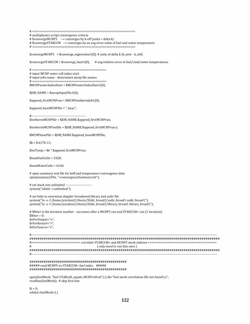
122
# ========================================================= # multiphysics script convergence criteria # $convergeMCNP5 --> converges by k-eff (units = delta k) # $convergeSTARCCM --> converges by an avg error value of fuel and water temperature # ========================================================= $convergeMCNP5 = $converge_eigenvalue1[0]; # units of delta k (k_new - k_old) $convergeSTARCCM = $converge_heat1[0]; # avg relative error in fuel/clad/water temperatures # ========================================= # input MCNP water cell index start # input jobs name - determines mcnp file names # ========================================= $MCNPwaterIndexStart = $MCNPwaterIndexStart1[0]; $JOB_NAME = $mcnpInputFile1[0]; $append_firstMCNPrun = $MCNPisothermJob1[0]; $append_baseMCNPfile = "_base"; #-------------------------------------------------- $isothermMCNPfile = $JOB_NAME.$append_firstMCNPrun; $isothermMCNPoutfile = $JOB_NAME.$append_firstMCNPrun.o; $MCNPbaseFile = $JOB_NAME.$append_baseMCNPfile; $k = 8.617E-11; $isoTemp = $k * $append_firstMCNPrun; $numFuelCells = 3328; $numWaterCells = 4160; # open summary text file for keff and temperature convergence data open(summaryFile, ">convergenceSummary.txt"); # set stack size unlimited ------------------------ system("ulimit -s unlimited"); # set links to enormous doppler broadened library and xsdir file system("ln -s -f /home/jcardoni2/thesis/XSdir_broad2/xsdir_broad1 xsdir_broad1"); system("ln -s -f /home/jcardoni2/thesis/XSdir_broad2/library_broad1 library_broad1"); # $Niter is the iteration number - increases after a MCNP5 run and STARCCM+ run (1 iteration) $Niter = 0; $oForOutput="o"; $rForRestart="r"; $sForSource="s"; # -------------------------------------------------------------------------------------------------------------------------------------------------------------------------- ############################################################################################## #>>>>>>>>>>>>>>>>>>>>>>>>>>> correlate STARCCM+ and MCNP5 mesh indexes <<<<<<<<<<<<<<<<<<<<<<<<<<<<<<<<<<<<<< # ( only need to run this once ) ############################################################################################## #--------------------------------------------------------------------------------------------------------------------------------------------------------------------------- ################################################ ##### read MCNP5-to-STARCCM+ fuel index ##### ################################################ open(fuelMesh, "fuel-STARcell_equals_MCNPcell.txt") || die "fuel mesh correlation file not found\n"; readline(fuelMesh); # skip first line $i = 0; while(<fuelMesh>) {

123
$i = $i + 1; $linevalues = $_; @values = split(" ",$linevalues); $fuelIndexSTAR[$i] = $values[0]; $fuelIndexMCNP[$i] = $values[2]; } close fuelMesh; ################################################ ##### read MCNP5-to-STARCCM+ water index ##### ################################################ open(waterMesh, "water-STARcell_equals_MCNPcell.txt") || die "water mesh correlation file not found\n"; readline(waterMesh); # skip first line $i = 0; while(<waterMesh>) { $i = $i + 1; $linevalues = $_; @values = split(" ",$linevalues); $waterIndexSTAR[$i] = $values[0]; $waterIndexMCNP[$i] = $values[2]; } close waterMesh; # -------------------------------------------------------------------------------------------------------------------------------------------------------------------------- ############################################################################################## ############################################################################################## # -------------------------------------------------------------------------------------------------------------------------------------------------------------------------- # prep mcnp post-processing specs file (for f90 post-processing code) $i = 0; open(specsBASE, "multiSpecs_base.txt") || die "multiSpecs_base.txt file not found\n"; @multispecsLines = <specsBASE>; close specsBASE; # open actual working java file with working directory in it open(MCNPspecs, ">multiSpecs.txt"); foreach $specsline (@multispecsLines) { $specsline =~ s/$JOB_NAME/$isothermMCNPfile/g; $specsline =~ s/$JOB_NAME$oForOutput/$isothermMCNPoutfile/g; print MCNPspecs $specsline; } close MCNPspecs; ################################################################## ##### load fuel isothermal material numbers and temperatures ##### ################################################################## $i=0; open (MCNPfile_base0, "$MCNPbaseFile") || die "base MCNP file not found\n"; while(<MCNPfile_base0>){ $i=$i+1; if (/f_$numFuelCells/) { $FUELlineNumberMax = $i; print "Loading isothermal fuel materials and $append_firstMCNPrun kT temps.\n"; } } seek(MCNPfile_base0,0,0); @mcnpBase0 = <MCNPfile_base0>; close MCNPfile_base0; $i = 0; foreach $line (@mcnpBase0) { $i=$i+1; $linearray[$i] = $line; }

124
$numberLines=$i; $j = 0; for ($i = 1; $i <= $FUELlineNumberMax; $i++) { if ($linearray[$i] =~ /f_/) { $j=$j+1; if ($j < 10 ) { $linearray[$i] =~ s/f_000$j/41/g; $linearray[$i] =~ s/ft000$j/$isoTemp/g; } elsif ($j < 100) { $linearray[$i] =~ s/f_00$j/41/g; $linearray[$i] =~ s/ft00$j/$isoTemp/g; } elsif ($j < 1000) { $linearray[$i] =~ s/f_0$j/41/g; $linearray[$i] =~ s/ft0$j/$isoTemp/g; } else { $linearray[$i] =~ s/f_$j/41/g; $linearray[$i] =~ s/ft$j/$isoTemp/g; } } } open (MCNPruntmp0, ">grid20cm_main293.tmp0"); for ($i = 1; $i <= $numberLines; $i++) { print MCNPruntmp0 $linearray[$i] ; } close MCNPruntmp0; ######################################################################## ##### load water isothermal material numbers, temps, and densities ##### ######################################################################## open (MCNPfile_base1, "grid20cm_main293.tmp0"); $i=0; $waterLookForNumber=$numWaterCells+$MCNPwaterIndexStart; while(<MCNPfile_base1>){ $i=$i+1; if (/w_$waterLookForNumber/) { $H20lineNumberMax = $i; print "Loading isothermal water materials and temperatures. \n"; } } seek(MCNPfile_base1,0,0); @mcnpBase1 = <MCNPfile_base1>; close MCNPfile_base1; $i = 0; foreach $line (@mcnpBase1) { $i=$i+1; $linearray[$i] = $line; } $j=$MCNPwaterIndexStart; for ($i = $FUELlineNumberMax; $i <= $H20lineNumberMax; $i++) { if ($linearray[$i] =~ /w_/) { $j=$j+1; $linearray[$i] =~ s/w_$j/43/g; $linearray[$i] =~ s/wden_$j/-1.0/g; $linearray[$i] =~ s/wt$j/$isoTemp/g; } } open (MCNPruntmp1, ">grid20cm_main293.tmp1"); for ($j = 1; $j <= $numberLines; $j++) { print MCNPruntmp1 $linearray[$j];

125
} close MCNPruntmp1; ################################################################## ##### load clad isothermal material numbers and temperatures ##### ################################################################## open (MCNPfile_base2, "grid20cm_main293.tmp1"); @mcnpBase2 = <MCNPfile_base2>; close MCNPfile_base2; open (MCNPruntmp2, ">$isothermMCNPfile"); foreach $line (@mcnpBase2) { $line =~ s/mclad/42/g; $line =~ s/cladt/$isoTemp/g; print MCNPruntmp2 $line ; } close MCNPruntmp2; system("chmod 775 *"); # remove temporary files system("rm grid20cm_main293.tmp*"); #^^^^^^^^^^^^^^^^^^^^^^^^^^^^^^^^^^^^^^^^^^^^^^^^^^^^^^^^^^^^^^^^^^^^^^^^^ #^^^^^^^^^^^^^^^^^^^^^^^^^^^^^^^^^^^^^^^^^^^^^^^^^^^^^^^^^^^^^^^^^^^^^^^^^ # run first MCNP5 job at isothermal conditions, uniform water density #-------------------------------------------------------------------------------------------- #^^^^^^^^^^^^^^^^^^^^^^^^^^^^^^^^^^^^^^^^^^^^^^^^^^^^^^^^^^^^^^^^^^^^^^^^^ #^^^^^^^^^^^^^^^^^^^^^^^^^^^^^^^^^^^^^^^^^^^^^^^^^^^^^^^^^^^^^^^^^^^^^^^^^ system("mpirun -n 4 mcnp5.mpi n=$isothermMCNPfile xsdir=xsdir_broad1"); # run f90 post processor to extract W/m^3 heat source # GETHEAT will create "heat.xy" file for STARCCM+'s java file to read in system("./GETHEAT"); # make sure all files are executable and readable system("chmod 775 *"); system("mv Heat.xy Heat_$Niter.xy"); system("mv RPDoutPut.txt RPDoutPut_$Niter.txt"); system("mv absoluteHeating.txt absoluteHeating_$Niter.txt"); system("mv fissionHeatingData.txt fissionHeatingData_$Niter.txt"); # extract k-eff from MCNP output file, calculate difference from previous iteration open(MCNPoutIsotherm, "$isothermMCNPoutfile") || die "MCNP5 isothermal output file missing for keff extraction.\n"; while(<MCNPoutIsotherm>) { if (/the final estimated combined collision/) { $keffLineString = $_; } } close MCNPoutIsotherm; @keffValues0 = split("=", $keffLineString); @keffValues1 = split(" ", $keffValues0[1]); $keff[$Niter] = $keffValues1[0]; $reactDk[$Niter] = $keff[$Niter] - $keff[$Niter-1]; $keff_diff[$Niter] = abs $reactDk[$Niter]; print "iso keff = $keff[$Niter] \n"; print summaryFile "iso keff = $keff[$Niter] \n";

126
#^^^^^^^^^^^^^^^^^^^^^^^^^^^^^^^^^^^^^^^^^^^^^^^^^^^^^^^^^^^^^^^^^^^^^^^^^ #^^^^^^^^^^^^^^^^^^^^^^^^^^^^^^^^^^^^^^^^^^^^^^^^^^^^^^^^^^^^^^^^^^^^^^^^^ # start main MULTINUKE “while” iteration loop ---> loops until convergence criteria satisfied #--------------------------------------------------------------------------------------------------------------------- #^^^^^^^^^^^^^^^^^^^^^^^^^^^^^^^^^^^^^^^^^^^^^^^^^^^^^^^^^^^^^^^^^^^^^^^^^ #^^^^^^^^^^^^^^^^^^^^^^^^^^^^^^^^^^^^^^^^^^^^^^^^^^^^^^^^^^^^^^^^^^^^^^^^^ use Cwd; $workdir = cwd; $keff_diff[$Niter] = 1000.0; $percentTemperatureDiff[$Niter] = 1000.0; while (($keff_diff[$Niter] > $convergeMCNP5) && ($percentTemperatureDiff[$Niter] > $convergeSTARCCM)) { open(STARJAVAFILE, "loadHeat_runStarJob_base.java") || die "STARCCM java base file not found, iteration = $Niter\n"; @starlines_array = <STARJAVAFILE>; close STARJAVAFILE; open(STARJAVANEW, ">loadHeat_runStarJob.java"); $NiterPlus1 = $Niter+1; foreach $starline (@starlines_array) { $starline =~ s/_WORKDIR_/$workdir/g; $starline =~ s/_ITERATION_/$Niter/g; $starline =~ s/_ITERATION1_/$NiterPlus1/g; print STARJAVANEW $starline; } close STARJAVANEW; system("chmod 775 *"); #^^^^^^^^^^^^^^^^^^^^^^^^^^^^^^^^^^^^^^^^^^^^^^^^^^^^^^^^^^^^^^^^^^^^^^^^^ #^^^^^^^^^^^^^^^^^^^^^^^^^^^^^^^^^^^^^^^^^^^^^^^^^^^^^^^^^^^^^^^^^^^^^^^^^ # run STARCCM+ with MCNP5 generated heat.xy file #--------------------------------------------------------------------------------------------------------------------- #^^^^^^^^^^^^^^^^^^^^^^^^^^^^^^^^^^^^^^^^^^^^^^^^^^^^^^^^^^^^^^^^^^^^^^^^^ #^^^^^^^^^^^^^^^^^^^^^^^^^^^^^^^^^^^^^^^^^^^^^^^^^^^^^^^^^^^^^^^^^^^^^^^^^ system("starccm+ -np 4 -batch loadHeat_runStarJob.java $JOB_NAME.sim"); system("mv $JOB_NAME\@04000.sim $JOB_NAME\@04000\_$NiterPlus1.sim"); $Niter = $Niter + 1; # kill script if max # of iterations exceeded if ($Niter > $iterationEnd) { die "maximum iterations exceeded. Sorry, I'm dead.\n"; } system("chmod 775 *"); #^^^^^^^^^^^^^^^^^^^^^^^^^^^^^^^^^^^^^^^^^^^^^^^^^^^^^^^^^^^^^^^^^^^^^^^^^ #^^^^^^^^^^^^^^^^^^^^^^^^^^^^^^^^^^^^^^^^^^^^^^^^^^^^^^^^^^^^^^^^^^^^^^^^^ # read in STARCCM+ output csv files, assign materials #------------------------------------------------------------------------- #^^^^^^^^^^^^^^^^^^^^^^^^^^^^^^^^^^^^^^^^^^^^^^^^^^^^^^^^^^^^^^^^^^^^^^^^^ #^^^^^^^^^^^^^^^^^^^^^^^^^^^^^^^^^^^^^^^^^^^^^^^^^^^^^^^^^^^^^^^^^^^^^^^^^ ########################################################### ##### read STARCCM+ fuel temperature output ##### ########################################################### open (STARtempDens_fuel, "STARCCMfuel_out\_$Niter.csv") || die "STARCCM fuel output file not found, iteration = $Niter\n"; readline(STARtempDens_fuel); $i = 0; while (<STARtempDens_fuel>) { $i = $i + 1; $linevalues = $_;

127
@values = split(" ",$linevalues); $FuelcellNum[$i] = $values[0]; $FuelcellTemp[$i][$Niter] = $values[2]; } $numFuelCells=$i; ### assign MCNP fuel material numbers for ($i = 1; $i <= $numFuelCells; $i++) { if ($FuelcellTemp[$i][$Niter] < 650) { # fuel bin 1: broadened to 625 K (600 K - 650 K) $FuelMat_Num[$i] = 1; } elsif (($FuelcellTemp[$i][$Niter] >= 650) && ($FuelcellTemp[$i][$Niter] < 700)) { # fuel bin 2: broadened to 675 K (650 K - 700 K) $FuelMat_Num[$i] = 2; } elsif (($FuelcellTemp[$i][$Niter] >= 700) && ($FuelcellTemp[$i][$Niter] < 750)) { # fuel bin 3: broadened to 725 K (700 K - 750 K) $FuelMat_Num[$i] = 3; } elsif (($FuelcellTemp[$i][$Niter] >= 750) && ($FuelcellTemp[$i][$Niter] < 800)) { # fuel bin 4: broadened to 775 K (750 K - 800 K) $FuelMat_Num[$i] = 4; } elsif (($FuelcellTemp[$i][$Niter] >= 800) && ($FuelcellTemp[$i][$Niter] < 850)) { # fuel bin 5: broadened to 825 K (800 K - 850 K) $FuelMat_Num[$i] = 5; } elsif (($FuelcellTemp[$i][$Niter] >= 850) && ($FuelcellTemp[$i][$Niter] < 900)) { # fuel bin 6: broadened to 875 K (850 K - 900 K) $FuelMat_Num[$i] = 6; } elsif (($FuelcellTemp[$i][$Niter] >= 900) && ($FuelcellTemp[$i][$Niter] < 950)) { # fuel bin 7: broadened to 925 K (900 K - 950 K) $FuelMat_Num[$i] = 7; } elsif (($FuelcellTemp[$i][$Niter] >= 950) && ($FuelcellTemp[$i][$Niter] < 1000)) { # fuel bin 8: broadened to 975 K (950 K - 1000 K) $FuelMat_Num[$i] = 8; } elsif (($FuelcellTemp[$i][$Niter] >= 1000) && ($FuelcellTemp[$i][$Niter] < 1050)){# fuel bin 9: broadened to 1025 K (1000 K - 1050 K) $FuelMat_Num[$i] = 9; } elsif (($FuelcellTemp[$i][$Niter] >= 1050) && ($FuelcellTemp[$i][$Niter] < 1100)){# fuel bin 10: broadened to 1075 K (1050K-1100 K) $FuelMat_Num[$i] = 10; } elsif (($FuelcellTemp[$i][$Niter] >= 1100) && ($FuelcellTemp[$i][$Niter] < 1150)){#fuel bin 11: broadened to 1125 K (110 K - 1150 K) $FuelMat_Num[$i] = 11; } elsif (($FuelcellTemp[$i][$Niter] >= 1150) && ($FuelcellTemp[$i][$Niter] < 1200)){#fuel bin 12: broadened to 1175 K (1150K -1200 K) $FuelMat_Num[$i] = 12; } elsif (($FuelcellTemp[$i][$Niter] >= 1200) && ($FuelcellTemp[$i][$Niter] < 1250)) {#fuel bin 13: broadened to 1225 K (1200K-1250 K) $FuelMat_Num[$i] = 13; } elsif (($FuelcellTemp[$i][$Niter] >= 1250) && ($FuelcellTemp[$i][$Niter] < 1300)){# fuel bin 14: broadened to 1275 K (1250K-1300 K) $FuelMat_Num[$i] = 14; } else { $FuelMat_Num[$i] = 15; # fuel bin 15: broadened to 1325 K (1300 K - 1350 K) } } ########################################################### ##### read STARCCM+ clad temperature output ##### ########################################################### open (STARtempDens_clad, "STARCCMclad_out\_$Niter.csv") || die "STARCCM clad output file not found, iteration = $Niter\n"; readline(STARtempDens_clad); $i = 0; while (<STARtempDens_clad>) { $i = $i + 1; $linevalues = $_;

128
@values = split(" ",$linevalues); $CladcellNum[$i] = $values[0]; $CladcellTemp[$i][$Niter] = $values[2]; $CladcellVolume[$i] = $values[3] * (10.0**6.0); # 1 m^3 = 1,000,000 cm^3 } $numCladCells=$i; ### calculate volume-weighted average clad temperature $totalCladVolume=0.0; for ($i = 1; $i <= $numCladCells; $i++) { $totalCladVolume = $totalCladVolume + $CladcellVolume[$i]; } $numerator_avgCladTemp=0.0; for ($i = 1; $i <= $numCladCells; $i++) { $numerator_avgCladTemp = $numerator_avgCladTemp + $CladcellTemp[$i][$Niter] * $CladcellVolume[$i]; } $avgCladTemp = $numerator_avgCladTemp / $totalCladVolume; ### assign MCNP clad material number if ($avgCladTemp < 600) { $CladMat_Num = 21; # clad bin 1: broadened to 550 K } elsif (($avgCladTemp >= 600) && ($avgCladTemp < 700)) { $CladMat_Num = 22; # clad bin 2: broadened to 650 K } else{ $CladMat_Num = 23; # clad bin 3: broadened to 750 K } ########################################################### ##### read STARCCM+ water density/temperature output ##### ########################################################### open (STARtempDens_water, "STARCCMwater_out\_$Niter.csv") || die "STARCCM water output file not found, iteration = $Niter\n"; readline(STARtempDens_water); $i = 0; while (<STARtempDens_water>) { $i = $i + 1; $linevalues = $_; @values = split(" ",$linevalues); $H2OcellNum[$i] = $values[0]; $H2OcellDens[$i] = $values[1] * 0.001*(-1.0); # convert kg/m^3 to g/cc, make negative for MCNP5 cell cards $H2OcellTemp[$i][$Niter] = $values[2]; } $numWaterCells=$i; $i = 0; close STARtempDens_water; ### assign MCNP water material numbers for ($i = 1; $i <= $numWaterCells; $i++) { if ($H2OcellTemp[$i][$Niter] < 560) { # water bin 1: broadened to 555.0 K (550 K - 560 K) $WaterMat_Num[$i] = 31; } elsif (($H2OcellTemp[$i][$Niter] >= 560) && ($H2OcellTemp[$i][$Niter] < 570)) { # water bin 2: broadened to 570.0 K (560 K -570 K) $WaterMat_Num[$i] = 32; } elsif (($H2OcellTemp[$i][$Niter] >= 570) && ($H2OcellTemp[$i][$Niter] < 575)) { # water bin 3: broadened to 572.5 K (570 K - 575 K)

129
$WaterMat_Num[$i] = 33; } elsif (($H2OcellTemp[$i][$Niter] >= 575) && ($H2OcellTemp[$i][$Niter] < 580)) { # water bin 4: broadened to 577.5 K (575 K - 580 K) $WaterMat_Num[$i] = 34; } elsif (($H2OcellTemp[$i][$Niter] >= 580) && ($H2OcellTemp[$i][$Niter] < 585)) { # water bin 5: broadened to 582.5 K (580 K - 585 K) $WaterMat_Num[$i] = 35; } elsif (($H2OcellTemp[$i][$Niter] >= 585) && ($H2OcellTemp[$i][$Niter] < 590)) { # water bin 6: broadened to 587.5 K (585 K - 590 K) $WaterMat_Num[$i] = 36; } elsif (($H2OcellTemp[$i][$Niter] >= 590) && ($H2OcellTemp[$i][$Niter] < 595)) { # water bin 7: broadened to 592.5 K (590 K - 595 K) $WaterMat_Num[$i] = 37; } elsif (($H2OcellTemp[$i][$Niter] >= 595) && ($H2OcellTemp[$i][$Niter] < 600)) { # water bin 8: broadened to 597.5 K (595 K - 600 K) $WaterMat_Num[$i] = 38; } else{ # water bin 9: broadened to 605.0 K (600 K - 610 K) $WaterMat_Num[$i] = 39; } } ######################################################################################## ##### calculate avg % difference in STAR cell temperatures from previous iteration ##### ######################################################################################## # avg relative error in fuel/water temperature distribution avg{ (T_new[i]-T_old[i]) / [(T_new[i]+T_old[i])/2] } $SUMfuel=0.0; for ($i = 1; $i <= $numFuelCells; $i++) { $FuelcellTemp[$i][0] = $append_firstMCNPrun; $FuelPercentDiff[$i] = abs( ($FuelcellTemp[$i][$Niter]-$FuelcellTemp[$i][$Niter-1]) / (($FuelcellTemp[$i][$Niter]+$FuelcellTemp[$i][$Niter-1])/2.0) ); } for ($i = 1; $i <= $numFuelCells; $i++) { $SUMfuel = $SUMfuel + $FuelPercentDiff[$i]; } $SUMclad=0.0; for ($i = 1; $i <= $numCladCells; $i++) { $CladcellTemp[$i][0] = $append_firstMCNPrun; $CladPercentDiff[$i] = abs( ($CladcellTemp[$i][$Niter]-$CladcellTemp[$i][$Niter-1]) / (($CladcellTemp[$i][$Niter]+$CladcellTemp[$i][$Niter-1])/2.0) ); } for ($i = 1; $i <= $numCladCells; $i++) { $SUMclad = $SUMclad + $CladPercentDiff[$i]; } $SUMwater=0.0; for ($i = 1; $i <= $numWaterCells; $i++) { $H2OcellTemp[$i][0] = $append_firstMCNPrun; $WaterPercentDiff[$i] = abs( ($H2OcellTemp[$i][$Niter]-$H2OcellTemp[$i][$Niter-1]) / (($H2OcellTemp[$i][$Niter]+$H2OcellTemp[$i][$Niter-1])/2.0) ); } for ($i = 1; $i <= $numWaterCells; $i++) { $SUMwater = $SUMwater + $WaterPercentDiff[$i]; } $AVGFuelPercentDiff = $SUMfuel/$numFuelCells; $AVGCladPercentDiff = $SUMclad/$numCladCells; $AVGWaterPercentDiff = $SUMwater/$numWaterCells; print "Iter = $Niter, Fuel%Diff = $AVGFuelPercentDiff, Clad%Diff = $AVGCladPercentDiff, Water%Diff = $AVGWaterPercentDiff\n"; print summaryFile "Iter = $Niter, Fuel%Diff = $AVGFuelPercentDiff, Clad%Diff = $AVGCladPercentDiff, Water%Diff = $AVGWaterPercentDiff\n"; $percentTemperatureDiff[$Niter] = ($AVGFuelPercentDiff+$AVGCladPercentDiff+$AVGWaterPercentDiff)/3.0; print "Iter = $Niter, percentTemperatureDiff = $percentTemperatureDiff[$Niter]\n";

130
print summaryFile "Iter = $Niter, percentTemperatureDiff = $percentTemperatureDiff[$Niter]\n"; ################################################ ##### load fuel material numbers and temps ##### ################################################ $i=0; open (MCNPfile_base0, "$MCNPbaseFile") || die "base MCNP file not found, iteration = $Niter\n"; while(<MCNPfile_base0>){ $i=$i+1; if (/f_$numFuelCells/) { $FUELlineNumberMax = $i; print "Loading fuel materials and temperatures. This will take a few seconds...\n"; } } seek(MCNPfile_base0,0,0); @mcnpBase0 = <MCNPfile_base0>; close MCNPfile_base0; $i = 0; foreach $line (@mcnpBase0) { $i=$i+1; $linearray[$i] = $line; } $numberLines=$i; for ($i = 1; $i <= $numFuelCells; $i++) { $FuelcellTempKT[$i] = $FuelcellTemp[$i][$Niter]*$k; } for ($i = 1; $i <= $numFuelCells; $i++) { for ($j = 1; $j <= $FUELlineNumberMax; $j++) { if ($fuelIndexMCNP[$i] < 10 ) { if ($linearray[$j] =~ s/f_000$fuelIndexMCNP[$i]/$FuelMat_Num[$i]/g) { $linearray[$j] =~ s/ft000$fuelIndexMCNP[$i]/$FuelcellTempKT[$i]/g; } } elsif ($fuelIndexMCNP[$i] < 100) { if ($linearray[$j] =~ s/f_00$fuelIndexMCNP[$i]/$FuelMat_Num[$i]/g) { $linearray[$j] =~ s/ft00$fuelIndexMCNP[$i]/$FuelcellTempKT[$i]/g; } } elsif ($fuelIndexMCNP[$i] < 1000) { if ($linearray[$j] =~ s/f_0$fuelIndexMCNP[$i]/$FuelMat_Num[$i]/g) { $linearray[$j] =~ s/ft0$fuelIndexMCNP[$i]/$FuelcellTempKT[$i]/g; } } else { if ($linearray[$j] =~ s/f_$fuelIndexMCNP[$i]/$FuelMat_Num[$i]/g) { $linearray[$j] =~ s/ft$fuelIndexMCNP[$i]/$FuelcellTempKT[$i]/g; } } } } open (MCNPruntmp0, ">$JOB_NAME.tmp0"); for ($j = 1; $j <= $numberLines; $j++) { print MCNPruntmp0 $linearray[$j] ; } close MCNPruntmp0; ############################################################# ##### load water material numbers, densities, and temps ##### ############################################################# open (MCNPfile_base1, "$JOB_NAME.tmp0"); $i=0; $waterLookForNumber=$numWaterCells+$MCNPwaterIndexStart; while(<MCNPfile_base1>){

131
$i=$i+1; if (/w_$waterLookForNumber/) { $H20lineNumberMax = $i; print "Loading water materials, densities, and temperatures. This will take a few seconds...\n"; } } seek(MCNPfile_base1,0,0); @mcnpBase1 = <MCNPfile_base1>; close MCNPfile_base1; $i = 0; foreach $line (@mcnpBase1) { $i=$i+1; $linearray[$i] = $line; } for ($i = 1; $i <= $numWaterCells; $i++) { $H2OcellTempKT[$i] = $H2OcellTemp[$i][$Niter]*$k; } for ($i = 1; $i <= $numWaterCells; $i++) { $waterIndexReplace[$i]=$waterIndexMCNP[$i]+$MCNPwaterIndexStart; for ($j = $FUELlineNumberMax; $j <= $H20lineNumberMax; $j++) { if ($linearray[$j] =~ s/w_$waterIndexReplace[$i]/$WaterMat_Num[$i]/g) { $linearray[$j] =~ s/wden_$waterIndexReplace[$i]/$H2OcellDens[$i]/g; $linearray[$j] =~ s/wt$waterIndexReplace[$i]/$H2OcellTempKT[$i]/g; } } } open (MCNPruntmp1, ">$JOB_NAME.tmp1"); for ($j = 1; $j <= $numberLines; $j++) { print MCNPruntmp1 $linearray[$j]; } close MCNPruntmp1; ################################################ ##### load clad material number ##### ################################################ open (MCNPfile_base2, "$JOB_NAME.tmp1"); @mcnpBase2 = <MCNPfile_base2>; close MCNPfile_base2; open (MCNPruntmp2, ">$JOB_NAME\_$Niter"); $avgCladTempKT = $avgCladTemp*$k; print "Loading clad materials and temperatures.\n"; foreach $line (@mcnpBase2) { $line =~ s/mclad/$CladMat_Num/g; $line =~ s/cladt/$avgCladTempKT/g; print MCNPruntmp2 $line ; } close MCNPruntmp2; system("chmod 775 *"); # remove temporary files system("rm $JOB_NAME.tmp*"); #^^^^^^^^^^^^^^^^^^^^^^^^^^^^^^^^^^^^^^^^^^^^^^^^^^^^^^^^^^^^^^^^^^^^^^^^^ #^^^^^^^^^^^^^^^^^^^^^^^^^^^^^^^^^^^^^^^^^^^^^^^^^^^^^^^^^^^^^^^^^^^^^^^^^ # rerun MCNP5 once with STARCCM+ output #------------------------------------------------------------------------- #^^^^^^^^^^^^^^^^^^^^^^^^^^^^^^^^^^^^^^^^^^^^^^^^^^^^^^^^^^^^^^^^^^^^^^^^^ #^^^^^^^^^^^^^^^^^^^^^^^^^^^^^^^^^^^^^^^^^^^^^^^^^^^^^^^^^^^^^^^^^^^^^^^^^

132
open(specsBASE, "multiSpecs_base.txt") || die "STARCCM java base file not found, iteration = $Niter\n"; @multispecsLines = <specsBASE>; close specsBASE; open(MCNPspecs, ">multiSpecs.txt"); foreach $specsline (@multispecsLines) { $specsline =~ s/$JOB_NAME/$JOB_NAME\_$Niter/g; $specsline =~ s/$JOB_NAME$oForOutput/$JOB_NAME\_$Niter$oForOutput/g; print MCNPspecs $specsline; } close MCNPspecs; system("mpirun -n 4 mcnp5.mpi n=$JOB_NAME\_$Niter xsdir=xsdir_broad1"); system("./GETHEAT"); system("chmod 775 *"); system("mv Heat.xy Heat_$Niter.xy"); system("mv RPDoutPut.txt RPDoutPut\_$Niter.txt"); system("mv absoluteHeating.txt absoluteHeating\_$Niter.txt"); system("mv fissionHeatingData.txt fissionHeatingData\_$Niter.txt"); system("rm $JOB_NAME\_$Niter$rForRestart"); system("rm $JOB_NAME\_$Niter$sForSource"); # extract k-eff from MCNP output file, calculate difference from previous iteration open(MCNPoutKeff, "$JOB_NAME\_$Niter$oForOutput") || die "MCNP5 output file missing for keff extraction. Iteration = $Niter\n"; while(<MCNPoutKeff>) { if (/the final estimated combined collision/) { $keffLineString = $_; } } close MCNPoutKeff; @keffValues0 = split("=", $keffLineString); @keffValues1 = split(" ", $keffValues0[1]); $keff[$Niter] = $keffValues1[0]; $reactDk[$Niter] = $keff[$Niter] - $keff[$Niter-1]; $keff_diff[$Niter] = abs $reactDk[$Niter]; print "iteration = $Niter, keff difference = $keff_diff[$Niter]\n"; print summaryFile "iteration = $Niter, keff difference = $keff_diff[$Niter]\n"; if (($keff_diff[$Niter] <= $convergeMCNP5) && ($percentTemperatureDiff[$Niter] <= $convergeSTARCCM)) { print summaryFile "Solutions appear converged. Ending MULTINUKE...\n"; print "Solutions appear converged. Ending MULTINUKE...\n"; close summaryFile; } } #closing bracket for iterating while loop in MULTINUKE

133
B.2 GETHEAT.f90 MCNP5 Post Processor
module data_constants
! ==================================================
! contains global variables, parameters
!
! ==================================================
integer :: io_number=0
integer, parameter :: fuelCellsPerNode=32
integer, parameter :: axialNodes=104
character (len=10), parameter :: specsFile='multiSpecs'
type paramStrings
! strings to look for that mark appropriate data in specs file
character (len=13) :: param1 = 'mcnpInputFile'
character (len=14) :: param2 = 'mcnpOutputFile'
character (len=12) :: param3 = 'rhoFuel_g_cc'
character (len=6) :: param4 = 'powerW'
character (len=15) :: param5 = 'Q_MeVperFission'
end type paramStrings
end module data_constants
module physicsData
! ==================================================
! model data: cell volumes, centroids
! ==================================================
real, dimension(32) :: vols_topNode = &
(/0.000134629, &
0.000645597, &
0.000663351, &
0.000151424, &
0.000147074, &
0.001356109, &
0.001490116, &
0.001490116, &
0.001355884, &
0.000140106, &
0.000670572, &
0.001490116, &
0.001490116, &
0.001490116, &
0.001490116, &
0.000665575, &
0.000668348, &
0.001490116, &
0.001490116, &
0.001490116, &
0.001490116, &
0.000665365, &
0.000146386, &
0.001357754, &
0.001490116, &
0.001490116, &
0.001356047, &
0.000140217, &
0.000135259, &
0.000646786, &
0.000663116, &
0.000151299/)
real, dimension(32) :: vols_bottomNode = &
(/0.000134629, &
0.000645597, &
0.000663351, &
0.000151424, &
0.000147074, &
0.001356109, &
0.001490116, &
0.001490116, &
0.001355884, &
0.000140106, &

134
0.000670572, &
0.001490116, &
0.001490116, &
0.001490116, &
0.001490116, &
0.000665575, &
0.000668348, &
0.001490116, &
0.001490116, &
0.001490116, &
0.001490116, &
0.000665365, &
0.000146386, &
0.001357754, &
0.001490116, &
0.001490116, &
0.001356047, &
0.000140217, &
0.000135259, &
0.000646786, &
0.000663116, &
0.000151299/)
real, dimension(32) :: vols_middleNodes = &
(/0.000717041, &
0.003304147, &
0.003320380, &
0.000719466, &
0.000717134, &
0.006679333, &
0.007450581, &
0.007450581, &
0.006739989, &
0.000690994, &
0.003276380, &
0.007450581, &
0.007450581, &
0.007450581, &
0.007450581, &
0.003299103, &
0.003286638, &
0.007450581, &
0.007450581, &
0.007450581, &
0.007450581, &
0.003318527, &
0.000710452, &
0.006739960, &
0.007450581, &
0.007450581, &
0.006777007, &
0.000694928, &
0.000709665, &
0.003265519, &
0.003325870, &
0.000754623/)
real, dimension(32) :: xc = &
(/ -0.231434, &
-0.089682, &
0.090564, &
0.233300, &
-0.412725, &
-0.286159, &
-0.097656, &
0.097656, &
0.285981, &
0.412210, &
-0.435431, &
-0.292969, &
-0.097656, &
0.097656, &
0.292969, &
0.435160, &
-0.435272, &
-0.292969, &

135
-0.097656, &
0.097656, &
0.292969, &
0.435118, &
-0.412474, &
-0.286230, &
-0.097656, &
0.097656, &
0.285989, &
0.412213, &
-0.231538, &
-0.089758, &
0.090536, &
0.233303/)
real, dimension(32) :: yc = &
(/ -0.411868, &
-0.433834, &
-0.434847, &
-0.413297, &
-0.233430, &
-0.285896, &
-0.292969, &
-0.292969, &
-0.286094, &
-0.232169, &
-0.089565, &
-0.097656, &
-0.097656, &
-0.097656, &
-0.097656, &
-0.089350, &
0.089444, &
0.097656, &
0.097656, &
0.097656, &
0.097656, &
0.089475, &
0.233648, &
0.285977, &
0.292969, &
0.292969, &
0.286101, &
0.232199, &
0.411906, &
0.433899, &
0.434837, &
0.413273/)
real, dimension(104) :: zc = &
(/ 0.00977585, &
0.07813705, &
0.2343784, &
0.4296904, &
0.62500245, &
0.82031445, &
1.0156264, &
1.21093845, &
1.4062505, &
1.60156245, &
1.7968744, &
1.99218635, &
2.1874983, &
2.38281035, &
2.5781224, &
2.7734344, &
2.9687464, &
3.16405845, &
3.3593705, &
3.5546825, &
3.7499945, &
3.94530655, &
4.1406186, &
4.3359306, &
4.5312426, &
4.7265546, &

136
4.92186665, &
5.11717845, &
5.3124902, &
5.50780225, &
5.7031143, &
5.8984263, &
6.0937383, &
6.28905035, &
6.4843624, &
6.6796744, &
6.8749864, &
7.0702984, &
7.26561045, &
7.4609225, &
7.6562345, &
7.8515465, &
8.0468583, &
8.24217035, &
8.43748235, &
8.63279435, &
8.8281064, &
9.02341845, &
9.21873045, &
9.41404245, &
9.6093545, &
9.80466655, &
9.99997855, &
10.19529055, &
10.3906026, &
10.58591465, &
10.78122665, &
10.97653865, &
11.1718507, &
11.36716225, &
11.56247425, &
11.75778625, &
11.95309825, &
12.1484103, &
12.34372235, &
12.53903435, &
12.73434635, &
12.9296584, &
13.12497045, &
13.32028245, &
13.51559445, &
13.7109065, &
13.90621855, &
14.10153055, &
14.29684255, &
14.4921546, &
14.68746665, &
14.88277865, &
15.0780902, &
15.27340225, &
15.46871425, &
15.66402625, &
15.8593383, &
16.05464985, &
16.24996185, &
16.44527435, &
16.64058685, &
16.8358984, &
17.03120995, &
17.22652245, &
17.42183495, &
17.6171465, &
17.81245805, &
18.00777055, &
18.20308305, &
18.3983946, &
18.59370615, &
18.78901865, &
18.98433115, &
19.1796427, &
19.37495425, &
19.57026675, &

137
19.7655783, &
19.92181875/)
end module physicsData
!\\\\\\\\\\\\\\\\\\\\\\\\\\\\\\\\\\\\\\\\\\\\\\\\\\\\\\\\\\\\\\\\\\\\\\\\\\\\\\\\\\\\\\\\
! ***************************************************************************************
!////////////////////////////////////////////////////////////////////////////////////////
Program getHeat
! ==================================================
! main program
!
! ==================================================
use data_constants
implicit none
logical :: exist_specsFile
character (len=60) :: mcnpInfile
character (len=60) :: mcnpOutfile
character :: tmp
character :: findequal = 'o'
real, dimension(4000) :: volume
real :: rhoFuel
real :: power
real :: Q_MeVperFiss
real :: eigenvalue
real :: Nu
inquire( file=specsFile//'.txt', exist=exist_specsFile )
if ( .not.exist_specsFile ) then
write(*,'(a,a,a)') 'Cannot find specs file: ',specsFile//'.txt',', exiting program.'
write(*,'(a)') 'Hit any key and enter to close.'
read(*,*)
call exit()
endif
call loadVolumes(volume) ! load mcnp cell volumes
call readSpecsInput(mcnpInfile,mcnpOutfile,rhoFuel,power,Q_MeVperFiss) ! read input
call axialPowerDist(mcnpInfile,mcnpOutfile,volume) ! extract axial power
call readEigenvalueNu(mcnpOutfile,eigenvalue,Nu) ! extract k-eff and Nu
call FissionHeating(mcnpInfile,mcnpOutfile,volume,rhoFuel,power,Q_MeVperFiss,eigenvalue,Nu)
write(*,*)
write(*,*) '*****************************************'
write(*,*) '*****************************************'
write(*,*)
write(*,*) 'Done reading heat.'
write(*,*)
end program getHeat
!\\\\\\\\\\\\\\\\\\\\\\\\\\\\\\\\\\\\\\\\\\\\\\\\\\\\\\\\\\\\\\\\\\\\\\\\\\\\\\\\\\\\\\\\
! ***************************************************************************************
!////////////////////////////////////////////////////////////////////////////////////////
subroutine readSpecsInput(mcnpInfile,mcnpOutfile,rhoFuel,power,Q_MeVperFiss)
! ==================================================
! extracts input data from multispecs.txt input file
! --> order of input data doesn't matter
! ==================================================
use data_constants
implicit none
type(paramStrings) :: specString
character (len=60), intent(out) :: mcnpInfile
character (len=60), intent(out) :: mcnpOutfile

138
character (len=60) :: tmp
character :: findequal='o'
real, intent(out) :: rhoFuel
real, intent(out) :: power
real, intent(out) :: Q_MeVperFiss
io_number=io_number+1
open( unit=io_number, file=specsFile//'.txt', status='old')
loop1: do while( .not.eof(io_number) )
do while( tmp /= specString%param1 )
if( eof(io_number) ) then
write(*,'(a,a,a)') 'Could not find ', specString%param1, ' in specs file, exiting', &
' program.'
write(*,'(a)') 'Hit any key and enter to close.'
read(*,*)
call exit()
endif
100 continue
read(io_number,'(a13)', advance='no', EOR=100) tmp
if( tmp == specString%param1) then
do while( findequal /= '=')
read(io_number,'(a)',advance='no') findequal
if( findequal == '=') then
read(io_number,'(1x,a60)') mcnpInfile
write(*,'(a,a)') 'Found mcnp input file in specs file ', mcnpInfile
endif
enddo
exit loop1
endif
enddo
enddo loop1
rewind(io_number)
findequal='o'
loop2: do while( .not.eof(io_number) )
do while( tmp /= specString%param2 )
if( eof(io_number) ) then
write(*,'(a,a,a)') 'Could not find ', specString%param2, ' in specs file, exiting', &
' program.'
write(*,'(a)') 'Hit any key and enter to close.'
read(*,*)
call exit()
endif
105 continue
read(io_number,'(a14)', advance='no', EOR=105) tmp
if( tmp == specString%param2) then
do while( findequal /= '=')
read(io_number,'(a)',advance='no') findequal
if( findequal == '=') then
read(io_number,'(1x,a60)') mcnpOutfile
write(*,'(a,a)') 'Found mcnp output file in specs file ', mcnpOutfile
endif
enddo
exit loop2
endif
enddo
enddo loop2
rewind(io_number)
findequal='o'
loop3: do while( .not.eof(io_number) )
do while( tmp /= specString%param3 )
if( eof(io_number) ) then
write(*,'(a,a,a)') 'Could not find ', specString%param3, ' in specs file, exiting', &
' program.'
write(*,'(a)') 'Hit any key and enter to close.'
read(*,*)
call exit()
endif
110 continue
read(io_number,'(a12)', advance='no', EOR=110) tmp
if( tmp == specString%param3) then
do while( findequal /= '=')
read(io_number,'(a)',advance='no') findequal
if( findequal == '=') then
read(io_number,*) rhoFuel

139
write(*,'(a,f)') 'Found fuel density = ', rhoFuel
endif
enddo
exit loop3
endif
enddo
enddo loop3
rewind(io_number)
findequal='o'
loop4: do while( .not.eof(io_number) )
do while( tmp /= specString%param4 )
if( eof(io_number) ) then
write(*,'(a,a,a)') 'Could not find ', specString%param4, ' in specs file, exiting', &
' program.'
write(*,'(a)') 'Hit any key and enter to close.'
read(*,*)
call exit()
endif
115 continue
read(io_number,'(a7)', advance='no', EOR=115) tmp
if( tmp == specString%param4) then
do while( findequal /= '=')
read(io_number,'(a)',advance='no') findequal
if( findequal == '=') then
read(io_number,*) power
write(*,'(a,f)') 'Found power = ', power
endif
enddo
exit loop4
endif
enddo
enddo loop4
rewind(io_number)
findequal='o'
loop5: do while( .not.eof(io_number) )
do while( tmp /= specString%param5 )
if( eof(io_number) ) then
write(*,'(a,a,a)') 'Could not find ', specString%param5, ' in specs file, exiting', &
' program.'
write(*,'(a)') 'Hit any key and enter to close.'
read(*,*)
call exit()
endif
120 continue
read(io_number,'(a15)', advance='no', EOR=120) tmp
if( tmp == specString%param5) then
do while( findequal /= '=')
read(io_number,'(a)',advance='no') findequal
if( findequal == '=') then
read(io_number,*) Q_MeVperFiss
write(*,'(a,f5.1)') 'Found MeV/fission = ', Q_MeVperFiss
endif
enddo
exit loop5
endif
enddo
enddo loop5
rewind(io_number)
findequal='o'
close(io_number)
end subroutine readSpecsInput
!\\\\\\\\\\\\\\\\\\\\\\\\\\\\\\\\\\\\\\\\\\\\\\\\\\\\\\\\\\\\\\\\\\\\\\\\\\\\\\\\\\\\\\\\
! ***************************************************************************************
!////////////////////////////////////////////////////////////////////////////////////////
subroutine loadVolumes(volume)
! ==================================================
! assigns volumes to mcnp cells
! ==================================================
use physicsData

140
use data_constants
implicit none
real, dimension(4000), intent(out) :: volume
integer :: i=0
integer :: n=0
integer :: z
!load in bottom volumes
do i = 1, fuelCellsPerNode
n=n+1
volume(n) = vols_bottomNode(i)
enddo
!load in middle volumes
do z = 2, axialNodes-1
do i = 1,fuelCellsPerNode
n=n+1
volume(n) = vols_middleNodes(i)
enddo
enddo
!load in top volumes
do i = 1, fuelCellsPerNode
n=n+1
volume(n) = vols_topNode(i)
enddo
end subroutine loadVolumes
!\\\\\\\\\\\\\\\\\\\\\\\\\\\\\\\\\\\\\\\\\\\\\\\\\\\\\\\\\\\\\\\\\\\\\\\\\\\\\\\\\\\\\\\\
! ***************************************************************************************
!////////////////////////////////////////////////////////////////////////////////////////
subroutine axialPowerDist(mcnpInfile,mcnpOutfile,volume)
! ==================================================
! extracts and prints axial power distribution
! ( point/avg fission reaction rates )
! ==================================================
use data_constants
implicit none
character (len=60), intent(in) :: mcnpInfile
character (len=60), intent(in) :: mcnpOutfile
real,dimension(4000),intent(in) :: volume
character (len=46) :: findFissionRxnRates
logical :: exist_mcnpOutfile
integer :: numFuelBins
integer :: i=0
integer :: z=0
integer :: n=0
integer :: radialStart=1
real, dimension(axialNodes) :: axialsum=0.0
real, dimension(4000) :: fission
real, dimension(4000) :: error
real :: avgFiss
real :: avgAxialFiss
real, dimension(4000) :: normPowerDist
real, dimension(axialNodes) :: axialFiss
real :: sum_Weighted_Fission=0.0
inquire( file=trim(mcnpOutfile), exist=exist_mcnpOutfile )
if ( .not.exist_mcnpOutfile ) then
write(*,'(a,a,a)') 'Cannot find mcnp output file for fission rxn rate: ',trim(mcnpOutfile), &
' exiting program.'
write(*,'(a)') 'Hit any key and enter to close.'
read(*,*)
call exit()
endif
io_number=io_number+1
open( unit=io_number, file=trim(mcnpOutfile), status='old' )
do while( .not.eof(io_number) )
read(io_number,'(a46)') findFissionRxnRates

141
if ( findFissionRxnRates == ' multiplier bin: 1.00000E+00 1 -6' ) then
i=i+1
read(io_number,'(17x,E11.5E3,1x,f6.4)') fission(i), error(i)
endif
enddo
numFuelBins = i
close(io_number)
do i = 1, numFuelBins
sum_Weighted_Fission = sum_Weighted_Fission + fission(i) * volume(i)
enddo
avgFiss = sum_Weighted_Fission /numFuelBins
!calculate 3d relative power distribution
do i = 1, numFuelBins
normPowerDist(i) = fission(i) * volume(i)/ avgFiss
enddo
radialStart=1
!integrate radially at each axial node
do z = 1, axialNodes
do i = radialStart, fuelCellsPerNode+radialStart-1
axialsum(z) = axialsum(z) + fission(i) * volume(i)
enddo
radialStart = radialStart + fuelCellsPerNode
enddo
avgAxialFiss = sum(axialsum) / axialNodes
!calculate normalized axial fission reaction rates
do z = 1, axialNodes
axialFiss(z) = axialsum(z) / avgAxialFiss
enddo
io_number=io_number+1
open( unit=io_number, file='RPDoutPut.txt')
do i = 1, numFuelBins
write(io_number,'(i4,a,f9.7)') i,' ', normPowerDist(i)
enddo
write(io_number,*)
write(io_number,*)
write(io_number,*)
do z = 1, axialNodes
write(io_number,'(a13,i3,a,f9.7)') 'axial node = ',z,' ',axialFiss(z)
enddo
close(io_number)
end subroutine axialPowerDist
!\\\\\\\\\\\\\\\\\\\\\\\\\\\\\\\\\\\\\\\\\\\\\\\\\\\\\\\\\\\\\\\\\\\\\\\\\\\\\\\\\\\\\\\\
! ***************************************************************************************
!////////////////////////////////////////////////////////////////////////////////////////
subroutine readEigenvalueNu(mcnpOutfile,eigenvalue,Nu)
! ==================================================
! read eigenvalue and Nu value from MCNP output file
! ==================================================
use data_constants
implicit none
character (len=60), intent(in) :: mcnpOutfile
real, intent(out) :: eigenvalue
real, intent(out) :: Nu
logical :: exist_mcnpOutfile
character (len=73) :: tmp
character (len=57) :: tmp2
inquire( file=trim(mcnpOutfile), exist=exist_mcnpOutfile )

142
if ( .not.exist_mcnpOutfile ) then
write(*,'(a,a,a)') 'Cannot find mcnp output file: ',trim(mcnpOutfile),', exiting program.'
write(*,'(a)') 'Hit any key and enter to close.'
read(*,*)
call exit()
endif
io_number=io_number+1
open( unit=io_number, file=trim(mcnpOutfile), status='old' )
loop10:do while( .not.eof(io_number) )
do while( tmp /= " | the final estimated combined collision/absorption/track-length keff = ")
if( eof(io_number) ) then
write(*,'(a)') 'getHeat.f90 :: Could not find keff in MCNP5 outpuf file.'
write(*,'(a)') 'Hit any key and enter to close.'
read(*,*)
call exit()
endif
200 continue
read(io_number,'(a73)', advance='no', EOR=200) tmp
if( tmp == " | the final estimated combined collision/absorption/track-length keff = ") then
read(io_number,'(f7.5)') eigenvalue
write(*,'(a,f7.5)') 'Found keff = ', eigenvalue
exit loop10
endif
enddo
enddo loop10
rewind(io_number)
loop11:do while( .not.eof(io_number) )
do while( tmp2 /= " | the average number of neutrons produced per fission = ")
if( eof(io_number) ) then
write(*,'(a)') 'getHeat.f90 :: Could not find Nu in MCNP5 outpuf file.'
write(*,'(a)') 'Hit any key and enter to close.'
read(*,*)
call exit()
endif
205 continue
read(io_number,'(a57)', advance='no', EOR=205) tmp2
if( tmp2 == " | the average number of neutrons produced per fission = ") then
read(io_number,'(f5.3)') Nu
write(*,'(a,f5.3)') 'Found Nu = ', Nu
exit loop11
endif
enddo
enddo loop11
close(io_number)
end subroutine readEigenvalueNu
!\\\\\\\\\\\\\\\\\\\\\\\\\\\\\\\\\\\\\\\\\\\\\\\\\\\\\\\\\\\\\\\\\\\\\\\\\\\\\\\\\\\\\\\\
! ***************************************************************************************
!////////////////////////////////////////////////////////////////////////////////////////
subroutine FissionHeating(mcnpInfile,mcnpOutfile,volume,rhoFuel,power,Q_MeVperFiss,eigenvalue,Nu)
! ==================================================
! extracts and prints fission energy deposition
! ==================================================
use physicsData
use data_constants
implicit none
character (len=60), intent(in) :: mcnpInfile
character (len=60), intent(in) :: mcnpOutfile
real,dimension(4000),intent(in) :: volume
real, intent(in) :: rhoFuel
real, intent(in) :: power
real, intent(in) :: Q_MeVperFiss
real, intent(in) :: eigenvalue
real, intent(in) :: Nu
character (len=17) :: findFissionHeating
character (len=6) :: findHeatCell
logical :: exist_mcnpOutfile
integer :: numFuelBins

143
integer :: i=0
integer :: z=0
integer :: n=1
integer :: radialStart=1
real, dimension(4000) :: heating
real, dimension(4000) :: heating_W_m3
real, dimension(4000) :: Heat_error
real, dimension(4000) :: absolute_Heat
real :: PwrFactor
real, parameter :: volConvert_cc_m3=10.0**-6
inquire( file=trim(mcnpOutfile), exist=exist_mcnpOutfile )
if ( .not.exist_mcnpOutfile ) then
write(*,'(a,a,a)') 'Cannot find mcnp output file: ',trim(mcnpOutfile),', exiting program.'
write(*,'(a)') 'Hit any key and enter to close.'
read(*,*)
call exit()
endif
! this loop will find the track length fission heating tally.
! It does not have a "multiplier bin" before each tally bin like the fission rxn rate tally (14)
io_number=io_number+1
open( unit=io_number, file=trim(mcnpOutfile), status='old' )
loop20: do while( .not.eof(io_number) )
read(io_number,'(a17)') findFissionHeating
if ( findFissionHeating == ' masses' ) then
do while(findHeatCell /= ' cell ')
read(io_number,'(a6)') findHeatCell
if (findHeatCell == ' cell ') then
exit loop20
endif
enddo
endif
enddo loop20
! read in the heat tally data
loop21: do while( findHeatCell == ' cell ')
i=i+1
read(io_number,'(17x,E11.5E3,1x,f6.4)') heating(i), Heat_error(i)
read(io_number,*) ! skip the empty blank line following the heat tally bin
read(io_number,'(a6)') findHeatCell
if (findHeatCell /=' cell ') then
exit loop21
endif
enddo loop21
numFuelBins = i
close(io_number)
! ***************************************************
! ***************************************************
! convert normalized MeV/g tally to real W/m^3 units
! ***************************************************
! ***************************************************
do i=1, numFuelBins
heating_W_m3(i) = ( heating(i)*power*Nu / (1.602e-13*Q_MeVperFiss*eigenvalue) ) &
* ( rhoFuel*(1/volConvert_cc_m3)*1.602e-13 )
enddo
! write 3d heat distribution data (not normalized to anything)
io_number=io_number+1
open(io_number, file='fissionHeatingData.txt')
do i=1, numFuelBins
write(io_number, '(i4,a,E13.7E2)') i,' ',heating(i)
enddo
close(io_number)
! calculate/write absolute heat source (Watts in each cell, not W/m^3)
do i = 1, numFuelBins
absolute_Heat(i) = heating_W_m3(i) * volume(i) * volConvert_cc_m3
enddo
PwrFactor = power / sum(absolute_Heat) ! keeps total power level constant for sake of correct
! temperature values for non-realistic reactivities
io_number=io_number+1
open(io_number, file='Heat.xy')
write(io_number,'(a)') "X Y Z Heat"

144
n = 1 ! count for heating array
do z = 1, axialNodes
do i= 1, fuelCellsPerNode
write(io_number,'(f10.6,f10.6,f10.6,a,E13.7E2)') xc(i)/100.0, yc(i)/100.0, zc(z)/100.0,' ',&
heating_W_m3(n)*PwrFactor
n=n+1
enddo
enddo
close(io_number)
io_number=io_number+1
open(io_number, file='absoluteHeating.txt')
do i = 1, numFuelBins
write(io_number, *) i,absolute_Heat(i)*PwrFactor
enddo
write(io_number,*)
write(io_number,*)
write(io_number,*) 'total absolute heat = ', sum(absolute_Heat)*PwrFactor, ' Watts'
close(io_number)
write(*,*) 'total absolute heat = ', sum(absolute_Heat)*PwrFactor, ' Watts'
end subroutine FissionHeating

145
B.3 STAR-CCM+ Java Script
// STAR-CCM+ macro: loadHeat_runStarJob.java package macro; import java.util.*; import star.common.*; import star.base.neo.*; import star.energy.*; public class loadHeat_runStarJob extends StarMacro { public void execute() { Simulation simulation_0 = getActiveSimulation(); // load in MCNP generated volumetric energy (heat) source FileTable fileTable_0 = (FileTable) simulation_0.getTableManager().createFromFile(resolvePath("_WORKDIR_/Heat__ITERATION_.xy")); // apply "Heat" data column to "fuel" region as energy source Region region_0 = simulation_0.getRegionManager().getRegion("fuel"); EnergyUserSource energyUserSource_0 = region_0.getValues().get(EnergyUserSource.class); energyUserSource_0.setMethod(XyzTabularScalarProfileMethod.class); ((XyzTabularScalarProfileMethod) energyUserSource_0.getMethod()).setTable(fileTable_0); ((XyzTabularScalarProfileMethod) energyUserSource_0.getMethod()).setData("Heat"); // run STARCCM+ job with MCNP generated fission heat source Solution solution_0 = simulation_0.getSolution(); solution_0.initializeSolution(); simulation_0.getSimulationIterator().run(true); // STARCCM+ job done - now create, fill, and export STARCCM+ generated density/temperature output // ************************************************************************************************ // xyzInternalTable_0 is the fuel region csv output table // ************************************************************************************************ XyzInternalTable xyzInternalTable_0 = simulation_0.getTableManager().createInternal(XyzInternalTable.class); xyzInternalTable_0.setPresentationName("Fuel_OutPut"); xyzInternalTable_0.getParts().setObjects(region_0);

146
xyzInternalTable_0.getParts().setObjects(region_0); // set primitive field functions to be used in each region for table output: fuel, clad, and water PrimitiveFieldFunction primitiveFieldFunction_0 = ((PrimitiveFieldFunction) simulation_0.getFieldFunctionManager().getFunction("LocalCellIndex")); PrimitiveFieldFunction primitiveFieldFunction_1 = ((PrimitiveFieldFunction) simulation_0.getFieldFunctionManager().getFunction("Density")); PrimitiveFieldFunction primitiveFieldFunction_2 = ((PrimitiveFieldFunction) simulation_0.getFieldFunctionManager().getFunction("Temperature")); PrimitiveFieldFunction primitiveFieldFunction_3 = ((PrimitiveFieldFunction) simulation_0.getFieldFunctionManager().getFunction("Volume")); CompiledFieldFunction compiledFieldFunction_0 = ((CompiledFieldFunction) simulation_0.getFieldFunctionManager().getFunction("Centroid_0")); CompiledFieldFunction compiledFieldFunction_1 = ((CompiledFieldFunction) simulation_0.getFieldFunctionManager().getFunction("Centroid_1")); CompiledFieldFunction compiledFieldFunction_2 = ((CompiledFieldFunction) simulation_0.getFieldFunctionManager().getFunction("Centroid_2")); xyzInternalTable_0.setFieldFunctions(new NeoObjectVector(new Object[] {primitiveFieldFunction_0, primitiveFieldFunction_1, primitiveFieldFunction_2, primitiveFieldFunction_3, compiledFieldFunction_0, compiledFieldFunction_1, compiledFieldFunction_2})); FieldFunctionColumnDescriptor fieldFunctionColumnDescriptor_0 = ((FieldFunctionColumnDescriptor) xyzInternalTable_0.getColumnDescriptor("Cell Index")); fieldFunctionColumnDescriptor_0.setPosition(0); FieldFunctionColumnDescriptor fieldFunctionColumnDescriptor_1 = ((FieldFunctionColumnDescriptor) xyzInternalTable_0.getColumnDescriptor("Density")); fieldFunctionColumnDescriptor_1.setPosition(1); FieldFunctionColumnDescriptor fieldFunctionColumnDescriptor_2 = ((FieldFunctionColumnDescriptor) xyzInternalTable_0.getColumnDescriptor("Temperature")); fieldFunctionColumnDescriptor_2.setPosition(2); FieldFunctionColumnDescriptor fieldFunctionColumnDescriptor_3 = ((FieldFunctionColumnDescriptor) xyzInternalTable_0.getColumnDescriptor("Volume")); fieldFunctionColumnDescriptor_3.setPosition(3); FieldFunctionColumnDescriptor fieldFunctionColumnDescriptor_4 = ((FieldFunctionColumnDescriptor) xyzInternalTable_0.getColumnDescriptor("Centroid: X-Component")); fieldFunctionColumnDescriptor_4.setPosition(4); FieldFunctionColumnDescriptor fieldFunctionColumnDescriptor_5 = ((FieldFunctionColumnDescriptor) xyzInternalTable_0.getColumnDescriptor("Centroid: Y-Component")); fieldFunctionColumnDescriptor_5.setPosition(5); FieldFunctionColumnDescriptor fieldFunctionColumnDescriptor_6 = ((FieldFunctionColumnDescriptor) xyzInternalTable_0.getColumnDescriptor("Centroid: Z-Component"));

147
fieldFunctionColumnDescriptor_6.setPosition(6); xyzInternalTable_0.setFieldFunctions(new NeoObjectVector(new Object[] {primitiveFieldFunction_0, primitiveFieldFunction_1, primitiveFieldFunction_2, primitiveFieldFunction_3, compiledFieldFunction_0, compiledFieldFunction_1, compiledFieldFunction_2})); fieldFunctionColumnDescriptor_0.setPosition(0); fieldFunctionColumnDescriptor_1.setPosition(1); fieldFunctionColumnDescriptor_2.setPosition(2); fieldFunctionColumnDescriptor_3.setPosition(3); fieldFunctionColumnDescriptor_4.setPosition(4); fieldFunctionColumnDescriptor_5.setPosition(5); fieldFunctionColumnDescriptor_6.setPosition(6); // ************************************************************************************************ // xyzInternalTable_1 is the cladding csv output table file // ************************************************************************************************ XyzInternalTable xyzInternalTable_1 = simulation_0.getTableManager().createInternal(XyzInternalTable.class); xyzInternalTable_1.setPresentationName("Clad_OutPut"); Region region_1 = simulation_0.getRegionManager().getRegion("clad"); xyzInternalTable_1.getParts().setObjects(region_1); xyzInternalTable_1.getParts().setObjects(region_1); xyzInternalTable_1.setFieldFunctions(new NeoObjectVector(new Object[] {primitiveFieldFunction_0, primitiveFieldFunction_1, primitiveFieldFunction_2, primitiveFieldFunction_3, compiledFieldFunction_0, compiledFieldFunction_1, compiledFieldFunction_2})); FieldFunctionColumnDescriptor fieldFunctionColumnDescriptor_7 = ((FieldFunctionColumnDescriptor) xyzInternalTable_1.getColumnDescriptor("Cell Index")); fieldFunctionColumnDescriptor_7.setPosition(0); FieldFunctionColumnDescriptor fieldFunctionColumnDescriptor_8 = ((FieldFunctionColumnDescriptor) xyzInternalTable_1.getColumnDescriptor("Density")); fieldFunctionColumnDescriptor_8.setPosition(1); FieldFunctionColumnDescriptor fieldFunctionColumnDescriptor_9 = ((FieldFunctionColumnDescriptor) xyzInternalTable_1.getColumnDescriptor("Temperature")); fieldFunctionColumnDescriptor_9.setPosition(2); FieldFunctionColumnDescriptor fieldFunctionColumnDescriptor_10 = ((FieldFunctionColumnDescriptor) xyzInternalTable_1.getColumnDescriptor("Volume")); fieldFunctionColumnDescriptor_10.setPosition(3);

148
FieldFunctionColumnDescriptor fieldFunctionColumnDescriptor_11 = ((FieldFunctionColumnDescriptor) xyzInternalTable_1.getColumnDescriptor("Centroid: X-Component")); fieldFunctionColumnDescriptor_11.setPosition(4); FieldFunctionColumnDescriptor fieldFunctionColumnDescriptor_12 = ((FieldFunctionColumnDescriptor) xyzInternalTable_1.getColumnDescriptor("Centroid: Y-Component")); fieldFunctionColumnDescriptor_12.setPosition(5); FieldFunctionColumnDescriptor fieldFunctionColumnDescriptor_13 = ((FieldFunctionColumnDescriptor) xyzInternalTable_1.getColumnDescriptor("Centroid: Z-Component")); fieldFunctionColumnDescriptor_13.setPosition(6); xyzInternalTable_1.setFieldFunctions(new NeoObjectVector(new Object[] {primitiveFieldFunction_0, primitiveFieldFunction_1, primitiveFieldFunction_2, primitiveFieldFunction_3, compiledFieldFunction_0, compiledFieldFunction_1, compiledFieldFunction_2})); fieldFunctionColumnDescriptor_7.setPosition(0); fieldFunctionColumnDescriptor_8.setPosition(1); fieldFunctionColumnDescriptor_9.setPosition(2); fieldFunctionColumnDescriptor_10.setPosition(3); fieldFunctionColumnDescriptor_11.setPosition(4); fieldFunctionColumnDescriptor_12.setPosition(5); fieldFunctionColumnDescriptor_13.setPosition(6); // ************************************************************************************************ // xyzInternalTable_2 is the water csv output table file // ************************************************************************************************ XyzInternalTable xyzInternalTable_2 = simulation_0.getTableManager().createInternal(XyzInternalTable.class); xyzInternalTable_2.setPresentationName("Water_OutPut"); Region region_2 = simulation_0.getRegionManager().getRegion("water"); xyzInternalTable_2.getParts().setObjects(region_2); xyzInternalTable_2.getParts().setObjects(region_2); xyzInternalTable_2.setFieldFunctions(new NeoObjectVector(new Object[] {primitiveFieldFunction_0, primitiveFieldFunction_1, primitiveFieldFunction_2, primitiveFieldFunction_3, compiledFieldFunction_0, compiledFieldFunction_1, compiledFieldFunction_2})); FieldFunctionColumnDescriptor fieldFunctionColumnDescriptor_14 = ((FieldFunctionColumnDescriptor) xyzInternalTable_2.getColumnDescriptor("Cell Index")); fieldFunctionColumnDescriptor_14.setPosition(0); FieldFunctionColumnDescriptor fieldFunctionColumnDescriptor_15 = ((FieldFunctionColumnDescriptor) xyzInternalTable_2.getColumnDescriptor("Density"));

149
fieldFunctionColumnDescriptor_15.setPosition(1); FieldFunctionColumnDescriptor fieldFunctionColumnDescriptor_16 = ((FieldFunctionColumnDescriptor) xyzInternalTable_2.getColumnDescriptor("Temperature")); fieldFunctionColumnDescriptor_16.setPosition(2); FieldFunctionColumnDescriptor fieldFunctionColumnDescriptor_17 = ((FieldFunctionColumnDescriptor) xyzInternalTable_2.getColumnDescriptor("Volume")); fieldFunctionColumnDescriptor_17.setPosition(3); FieldFunctionColumnDescriptor fieldFunctionColumnDescriptor_18 = ((FieldFunctionColumnDescriptor) xyzInternalTable_2.getColumnDescriptor("Centroid: X-Component")); fieldFunctionColumnDescriptor_18.setPosition(4); FieldFunctionColumnDescriptor fieldFunctionColumnDescriptor_19 = ((FieldFunctionColumnDescriptor) xyzInternalTable_2.getColumnDescriptor("Centroid: Y-Component")); fieldFunctionColumnDescriptor_19.setPosition(5); FieldFunctionColumnDescriptor fieldFunctionColumnDescriptor_20 = ((FieldFunctionColumnDescriptor) xyzInternalTable_2.getColumnDescriptor("Centroid: Z-Component")); fieldFunctionColumnDescriptor_20.setPosition(6); xyzInternalTable_2.setFieldFunctions(new NeoObjectVector(new Object[] {primitiveFieldFunction_0, primitiveFieldFunction_1, primitiveFieldFunction_2, primitiveFieldFunction_3, compiledFieldFunction_0, compiledFieldFunction_1, compiledFieldFunction_2})); fieldFunctionColumnDescriptor_14.setPosition(0); fieldFunctionColumnDescriptor_15.setPosition(1); fieldFunctionColumnDescriptor_16.setPosition(2); fieldFunctionColumnDescriptor_17.setPosition(3); fieldFunctionColumnDescriptor_18.setPosition(4); fieldFunctionColumnDescriptor_19.setPosition(5); fieldFunctionColumnDescriptor_20.setPosition(6); // ************************************************************************************************ // export STARCCM+ generated temperature/density output for subsequent MCNP5 execution // ************************************************************************************************ xyzInternalTable_0.export(resolvePath("_WORKDIR_/STARCCMfuel_out__ITERATION1_.csv"), 0); xyzInternalTable_1.export(resolvePath("_WORKDIR_/STARCCMclad_out__ITERATION1_.csv"), 0); xyzInternalTable_2.export(resolvePath("_WORKDIR_/STARCCMwater_out__ITERATION1_.csv"), 0); } }

150
APPENDIX C. Data File Formats
C.1 MCNP5 to STAR-CCM+: Heat.xy Volumetric Heat Source File Excerpt
Below, (X,Y,Z) is the centroid of the MCNP5 cell in meters. Heat is the power density in each
cell in W/m3.
X Y Z Heat
-0.002314 -0.004119 0.000098 0.5730506E+08
-0.000897 -0.004338 0.000098 0.4047297E+08
0.000906 -0.004348 0.000098 0.3333602E+08
0.002333 -0.004133 0.000098 0.5421250E+08
-0.004127 -0.002334 0.000098 0.4626177E+08
-0.002862 -0.002859 0.000098 0.2874447E+08
-0.000977 -0.002930 0.000098 0.2483536E+08
0.000977 -0.002930 0.000098 0.2358711E+08
0.002860 -0.002861 0.000098 0.2792769E+08
0.004122 -0.002322 0.000098 0.5138924E+08
-0.004354 -0.000896 0.000098 0.3456092E+08
-0.002930 -0.000977 0.000098 0.2431238E+08
-0.000977 -0.000977 0.000098 0.2438148E+08
0.000977 -0.000977 0.000098 0.2386235E+08
0.002930 -0.000977 0.000098 0.2694028E+08
0.004352 -0.000893 0.000098 0.3700510E+08
-0.004353 0.000894 0.000098 0.3218361E+08
-0.002930 0.000977 0.000098 0.2638603E+08
-0.000977 0.000977 0.000098 0.2515003E+08
0.000977 0.000977 0.000098 0.2425299E+08
0.002930 0.000977 0.000098 0.2453624E+08
0.004351 0.000895 0.000098 0.3629155E+08
-0.004125 0.002336 0.000098 0.5619471E+08
-0.002862 0.002860 0.000098 0.2699767E+08
-0.000977 0.002930 0.000098 0.2517076E+08
0.000977 0.002930 0.000098 0.2657661E+08
0.002860 0.002861 0.000098 0.2698103E+08
0.004122 0.002322 0.000098 0.6107013E+08
-0.002315 0.004119 0.000098 0.6315418E+08
-0.000898 0.004339 0.000098 0.3628746E+08
0.000905 0.004348 0.000098 0.3516224E+08
0.002333 0.004133 0.000098 0.5715716E+08
-0.002314 -0.004119 0.000781 0.7674357E+08
-0.000897 -0.004338 0.000781 0.4743583E+08
0.000906 -0.004348 0.000781 0.4584070E+08
0.002333 -0.004133 0.000781 0.7622444E+08
-0.004127 -0.002334 0.000781 0.7234044E+08
-0.002862 -0.002859 0.000781 0.3797202E+08
-0.000977 -0.002930 0.000781 0.3304345E+08
0.000977 -0.002930 0.000781 0.3324944E+08
0.002860 -0.002861 0.000781 0.3678525E+08
0.004122 -0.002322 0.000781 0.7878394E+08
-0.004354 -0.000896 0.000781 0.4902124E+08
-0.002930 -0.000977 0.000781 0.3411621E+08
-0.000977 -0.000977 0.000781 0.3059442E+08
0.000977 -0.000977 0.000781 0.3184674E+08
0.002930 -0.000977 0.000781 0.3545682E+08
0.004352 -0.000893 0.000781 0.4881287E+08
-0.004353 0.000894 0.000781 0.4939116E+08
-0.002930 0.000977 0.000781 0.3251755E+08

151
C.2 STAR-CCM+ to MCNP5: CSV Temperature and Density Data File Excerpt
The CSV files are automatically generated by STAR-CCM+ with assistance from the Java script
(Appendix B.3). The headers at the top of the CSV files describe the quantity and units given in
each column.

152
APPENDIX D. Running MULTINUKE: An Overview of the Required Files
Figure 33 is a screen shot of a directory containing all the files required to run a MULTINUKE
simulation. Table 17 describes each file required to be located in the working directory to run
MULTINUKE. A comparable setup should allow the user to execute the MULTINUKE code,
assuming the user has made the necessary preparations to the MCNP5 input file, STAR-CCM+
simulation file and Java script, mesh correlation files, and the multiSpecs_base.txt file (as
described in Chapter 5, Section 5.2: Solver Preparation). Furthermore, the example directory
assumes the user has created a temperature dependent cross section library, and has proper
access to MCNP5 and STAR-CCM+ parallel executables. Depending on the operating system
settings, the user may be required to manually set the stacksize to unlimited to allow sufficient
memory allocation for MCNP5 and STAR-CCM+.
The MULTINUKE coupled solver is executed by running the Perl script:
./runMultiNuke.pl
Figure D1. Example of Working Directory for Running MULTINUKE.
Table D1. Required Files in MULTINUKE Working Directory.
File Name Description
fuel-STARcell_equals_MCNPcell.txt Fuel mesh correlation file.
GETHEAT Fortran90 post-processor for MCNP5.
loadHeat_runStarJob_base.java Base Java script for STAR-CCM+.
multiSpecs_base.txt Input file for MULTINUKE.
pin20cm_base MCNP5 base input file.
pin20cm.sim STAR-CCM+ simulation file.
runMultiNuke.pl Main MULTINUKE Perl Script.
water-STARcell_equals_MCNPcell.txt Coolant mesh correlation file.

153
Author’s Biography
Jeffrey Neil Cardoni was born on October 15, 1984. He graduated from Normal Community
West High School in 2003. In 2007, he earned a Bachelor of Science in Nuclear Engineering
from the University of Illinois at Urbana-Champaign, graduating with highest honors. After
working in various DOE laboratories, he returned to graduate school in 2009 to obtain an MS in
Nuclear Engineering from the University of Illinois.